demand forecasting - irc :: home · the "demand forecasting" module includes an overview...

7 5

5 D E

"VSTl-TV** ^

Instructor Guide Demand Forecasting

. . I .1 , , " • • » ! . ' . •

uvi'-.-.ixbiATIOiNiAI. REFERENCE CEMT7;

, - , - - . I ; . - / . . ; - . : v . / . - • • • •

, Ban* for construction and

19S5 by the international Bank

Copyright © ^ f rishts reserved. 2 ^ Development. «*

a^^oe-^io!

DEMAND FORECASTING

Instructor Guide

' UdFJAEY, iKTEfVMAT: : r / \ ! r.-"-:-' : ' c.-:••.•••••': : : O F ? cok :v , - . ..;•.•.' v.",- : ' AMD C ' i VfAVlOM ,l,\-.::) * P.O. L--..:; VJ"'SO, 2t>09 AD The 1 i Tel. (O/o) 814911 ext 141/142

!L0: ^ ^ 5 &5^£

J«

.<>•«

For additional information please write to: The Economic Development Institute of

The World Bank Studies Unit 1818 "H" Street, N.W. . Washington, D.C. 20433

n .«

GENERAL INFORMATION FOR THE INSTRUCTOR

Module Use and Content

The "Demand Forecasting" module may be used as an independent instructional unit, or in conjunction with the other modules in EDI's two-week seminar on "Water Supply and Sanitation." The module includes the following presentation materials:

• An Instructor Guide • A Participant Manual • A slide/tape program

Time Required

The module is divided into four parts and requires approximately six hours to complete.

Participant Manual and Instructor Guide

The Participant Manual contains all the information and instructions required to complete the module activities.

The Instructor Guide is organized so that Instructor Notes appear on the left-hand pages, opposite the Participant Manual pages printed on the right. (The Participant Manual pages in the Instructor Guide are identical to those in the actual Participant Manual.) The Instructor Notes include suggested time requirements, steps for conducting the module activities, discussion guidelines and suggestions on presentation. The time requirements are approximate, but following the suggested times will ensure that the module does not require more than six hours to complete.

The Instructor Guide and Participant Manual both contain reference copies of the visuals and the narrative text from the slide/tape program.

Slide/Tape Program

Most of the instructional content for this module is presented in the slide/tape program, "Demand Forecasting." The slide/tape program includes 160 35mm slides which are synchronized with the narration on two accompanying audiocassettes.

The slides are inserted in carousel trays that most projectors will accommodate. The narration for Parts I and II is on the first audiocassette. The narration for Parts III and IV is one the second audiocassette. Both audiocassettes are pulsed with audible tones. These tones are cues that the slide projector should be advanced immediately to the next slide.

i

Eqqipment and Materials

Presentation of the module by an instructor to a group of participants requires the equipment and materials listed below:

For the instructor: For the participants:

• One copy of the Instructor • A copy of the Participant Guide Manual for each participant

• A flipchart easel, pad and • Paper and pencils for each markers, or chalkboard and participant chalk

• One copy of the slide/tape program (slides and audio-cassettes)

• One slide projector and white projection screen

• One audiocassette player

Instructor Preparation

The "Demand Forecasting" module is not a self-instructional program. It requires an instructor who is knowledgeable about demand forecasting methods and applications.

Instructor preparation involves a review of the Instructor Guide to become familiar with the topics, the sequence of activities and the content of the presentations. It is also useful to preview the slide/tape program in order to become familiar with the content and the synchronization of the slides with the audiocassettes. If possible, the program should be previewed on the equipment that will be used during the actual presentation.

Equipment and Facilities Preparation

Preparation of the audiocassettes for play requires rewinding them completely to the beginning. When the cassettes are loaded into the player, Side 1 should show at the top.

Preparation of the carousel trays of slides for viewing requires four steps. First, it is important to ensure that all of the slides are inserted into the tray in sequential order, with the printed numbers showing at the top right corner, along the outer edge of the carousel tray. Second, the black plastic lock ring must be turned in the

11

direction of the arrow marked "Lock" until the ring is secured on the tray. Third, the tray is placed in the operating position by lowering it onto the the projector and turning it clockwise until the tray drops down securely. Fourth, the projector must be advanced so the first slide, the title slide, appears on the screen.

Operation of the slide projector and audiocassette player should be checked prior to the presentation. At that time, it is advisable to arrange for power cords required to operate the projector and the cassette player, extension cords and extra projector bulbs. It is also useful to determine who should be contacted if assistance is needed from an engineer or audiovisual specialist.

It is important to check that each participant will be able to see and hear the slide/tape program easily. To view the slides clearly, overhead and back lighting should be kept to a minimum.

i n

INSTRUCTOR NOTES

Overview

The "Demand Forecasting" module includes an overview of the characteristics of demand, the determinants of demand, and forecasting methods.

The module is divided into four parts. Each part includes one segment of the slide/tape program and at least one application activity to reinforce important concepts.

Most of the activities are conducted best in small groups of five to seven participants. If the participants are not divided into small groups, you may want to do so before proceeding with the module.

Introduction Time required: 15 minutes

1. Refer the participants to the Introduction on page 1 in their manuals. Review the purpose of the module and the topic outline with them.

2. Ask the participants to describe their past experience with demand forecasting in project selection or planning. Then ask them to describe their objectives in learning about demand forecasting and how they intend to use the information. Knowing about their experience and their objectives will help you relate the content of the module to their needs.

3. Tell the participants that they will not have to take extensive notes during the slide/tape program. Their manuals include copies of the visuals and the narration text from the slide/tape program as well as summaries of all major concepts presented.

4. .Introduce Part I of the slide tape program and inform the participants that it is the first of four parts. Explain that Part I includes an overview of the module and a review of the characteristics of demand. Part I of the slide/tape program is approximately ten minutes in length.

5. Turn on the equipment and make sure the title slide is projected before you turn on the audiocassette player. When you turn on the audiocassette player, the music at the start of the program will begin. When you hear the first tone, advance the slide projector immediately to the next slide. Continue advancing the slides at the sound of the tone until the narrator announces the end of Part I and you see a corresponding message projected on the screen.

I - 1

Introduction

The "Demand Forecasting" module has been designed for individuals who have a role in project planning or selection and who need a general orientation to the techniques of demand forecasting.

The module includes a review of the topics that are listed below.

PART I Overview of the module

CHARACTERISTICS OF DEMAND

Types of Demand Measurement of Demand Distribution of Consumption

PART II DETERMINANTS OF DEMAND

Price Metering

PART III Income Service Level Other Factors

PART IV FORECASTING METHODS

Requirements Method Exponential Method Explanatory Method

Sensitivity Analysis

P - 1

INSTRUCTOR NOTES

PART I; CHARACTERISTICS OF DEMAND

Review of the Characteristics of Demand Time required: 15 minutes

1. After the participants have viewed the first part of the slide/tape program, ask them if they have any questions about the content.

2. Ask the participants to turn to page 2 and review the summary information on pages 2, 3 and 4.

1 - 2

PAST I: CHARACTERISTICS OF DEMAND

Review of the Characteristics of Demand

Types of Demand

Water consumed is categorized according to the type of activity for which it is used. As a result, in most communities, there are four types of demand, including:

• Domestic demand for water at home;

• Commercial demand for service-oriented areas;

• Industrial demand for treated water; and

• Public sector demand for water for hospitals and schools.

Measurement of Consumption

Consumption of water by a community is usually expressed as:

• Average daily demand - the result when total annual consumption

is divided by the 365 days of the year.

There are two variations to average daily demand:

• Maximum daily demand - the consumption level on the day of the year when consumption is the highest; and

• Peak hour demand - the consumption level during the hour(s) of the day when consumption is the highest

When average daily demand is set at 100%, maximum daily demand is approximately 120% of average daily demand. Peak hour demand is approximately 180% of average daily demand.

P - 2

INSTRUCTOR NOTES

Review of the Characteristics of Demand (continued)

To

<W

I -3


The table below lists the average and maximum daily demand for several representative cities.

City

Population in Thousands

(December 1969)

Water Consumption from Municipal Water Supply (in liters per capita

per day) Average Maximum

Maximum Demand as a % of Average Daily Demand

Montreal, Canada 1,460 Los Angeles, U.S.A. 2,960 Tokyo, Japan 8,980 Brussels, Belgium 1,280 Amsterdam, Holland 830 Stuttgart, West Germany 620 Oslo, Norway 490 Stockholm, Sweden 760 London, England 6,060 Paris, France 2,580 Nairobi, Kenya 700

650 620 470 140 200 220 610 450 290 320 105

910 980 560 160 260 340 760 610 350 400 118

141% 159% 118% 111% 134% 151% 126% 136% 124% 127% 113%

Unaccounted Water

It is also important to take into account the difference between the amount of water produced and the amount that is consumed. The difference between the two is termed unaccounted water. Usually unaccounted water is expressed as a percentage of the amount of water produced. In order to calculate unaccounted water, two steps are required:

1. Subtract consumption from production. 2. Divide the remainder by production.

An efficient water supply system is one where unaccounted water is 20% or less. In order to forecast supply, it is necessary to add an amount for unaccounted water to consumption forecasts. For example, if Q represents consumption, water production will have to equal 3 Q if unaccounted water is 67%. When unaccounted water is 50%, the level of production will have to be 2Q, and so on.

P - 3

INSTRUCTOR NOTES


<*)

4. After you complete the review, ask. the participants to turn to page 5. *>

ft

«.*')

I -4


Distribution of Demand

Metering data is a source of information for compiling statistics on the distribution of consumption in a community. In the example below, the community's house connections are divided into increments of 10%, or deciles. Each decile is shown with its share of consumption.

Share of Consumers

The The The The The The The The The The

first second third fourth fifth sixth seventh eighth ninth tenth

10% 10% 10% 10% 10% 10% 10% 10% 10% 10%

Share of Consumption

Consume Consume Consume Consume Consume Consume Consume Consume Consume Consume

3% 3% 3% 4% 4% 5% 8% 13% 20% 35%

P -4

INSTRUCTOR NOTES

Calculating the Distribution of Consumption Time required: 40 minutes

1. Tell the participants that the next activity will provide thera with an opportunity to calculate the distribution of consumption in a community.

2.

3.

4.

Review the information and instructions with the participants.

Ask them to work with the members of their group to calculate the percentages and to record them in the space provided on page 5. Then instruct them to plot the data on the graph on page 6.

After 30 minutes, ask a representative of one group to present the group's calculations. Ask the other groups to review the numbers and to correct any, if necessary. The correct calculations are shown below. (The correct graph is on the following Instructor. Notes page.)

Consumer Group

0 - 5 5 - 7 7 - 9 9 - 1 1 11- 13 13- 15 15- 20 20- 30 . 30- 40 40- 60 60- 90 90- 150 150-210 210-300 300-600 600-900 900 +

TOTAL

Number of Consumers

1,060 670 920

1,700 1,340 1,380 3,550 3,680 1,550 1,360 560 260 90 60 80 20 20

18,300

% of Consumers

5.8 3.6 5.0 9.3 7.3 7.5 19.5 20.1 8.5 7.4 3.1 1.4 0.5 0.3 0.5 0.1 0.1

100.0%

Cumulative % of

Consumers

5.8 9.4 14.4 23.7 31.0 38.5 58.0 78.1 86.6 94.0 97.1 98.5 99.0 99.3 99.8 99.9 100.0

100.0%

Volume Consumed

2,300 4,900 9,200

21,900 21,000 24,500 83,300 121,200 79,300 88,200 53,500 38,500 22,000 20,600 46,000 18,700 108,400

763,500

% of Volume

0.3 0.6 1.2 2.9 2.7 3.2 11.0 15.9 10.4 11.6 7.0 5.0 2.9

' 2.7 6.0 2.4 14.2

100.0%

Cumulative % of

Volume

0.3 0.9 2.1 5.0 7.7 10.9 21.9 37.8-48.2 59.8 66.8 71.8 74.7 77.4 83.4 85.8 100.0

100.0%

1 - 5

Calculating the Distribution of Consumption

In this activity, you will calculate the distribution of consumption in a community. The community's consumers are divided into groups according to their consumption in cubic meters per month.

First, work, with the members of your group to calculate the total number of consumers. Record the total at the bottom of the column titled "Number of Consumers."

Second, calculate the percentage of consumers in each group by dividing the number of consumers in each group by the total number of consumers. Record those percentages in the column titled "Percentage of Consumers."

Third, calculate the cumulative distribution of consumers by adding the percentage consumption of each group to the cumulative percentage of the groups that preceed it. Record the cumulative percentages in the column titled "Cumulative Percentage of Consumers."

Fourth, calculate the total volume and record that number at the bottom of the column titled "Volume Consumed."

Fifth, calculate the percentage of volume consumed by each group and the cumulative percentage volume consumed. Record the percentages under the columns "Percentage of Volume" and "Cumulative Percentage of Volume."

Consumer Group

0 - 5 5 - 7 7 - 9 9 - 1 1 11 - 13 13 - 15 15 - 20 20 - 30 30 - 40 40 - 60 60 - 90 90 -150 150-210 210-300 300-600 600-900 900 +

TOTAL

Cumulative Number of % of % of Consumers Consumers Consumers

1,060 670 920

1,700 1,340 1,380 3,550 3,680 1,550 1,360 560 260 90 60 80 20

20

100.0% 100.0%

Cumulative Volume % of % of Consumed Volume Volume

2,300 4,900 9,200 21,900 21,000 24,500 83,300 121,200 79,300 88,200 53,500 38,500 22,000 20,600 46,000 18,700

108,400

100.0% 100.0%

P - 5

INSTRUCTOR NOTES

Calculating the Distribution of Consumption (continued)

5. Review the correct graph, shown below, with the participants.

auwjusnvx JWtCBNTACS or vovjm OONSUMED

-

- .. . ... : i«ox-

" BO* *

7 0 X -

irQt "

sox-

*ot-

30S-

201 .

101-

OX r i r t t i 1 1 r 101 201 301 401 SOX 60S 70S SOS 90S 100S

CUMULATIVE PDtCESTAGE OF CONSUMERS

Assist the participants to identify ways that they can use statistical data on the distribution of consumption for the projects with which they work.

Introduce Part II of the slide/tape program and tell the participants that it includes a review of the determinants of demand. Turn on the projector and make sure the title slide announcing Part II is projected. When you turn on the audiocassette player you will hear a signal tone and the music will begin. When you hear the next signal tone, advance the projector to the next slide. Continue advancing the projector at the sound of the tone until the narrator announces the end of Part II and you see a corresponding message projected on the screen. Part II is approximately eight minutes in length.

1 - 6

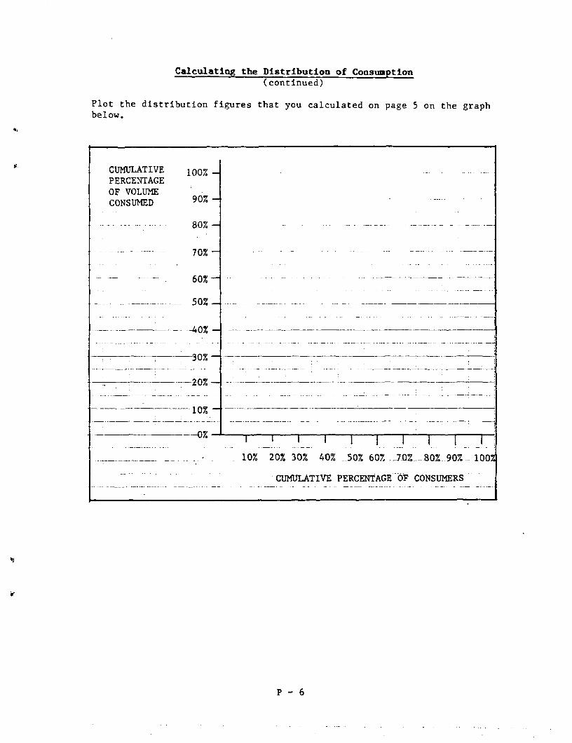
Calculating the Dis tr ibut ion of Consumption (continued)

Plot the distribution figures that you calculated on page 5 on the graph below.

CUMULATIVE PERCENTAGE OF VOLUME CONSUMED

- 100%

90%

80%-

70%-

60%

50%

--40%

-30%

---20%

10%

0% i J i i—i i i I — r ~ T 10% 20% 30% 40% .50% 60% .J7_QZ._-8Q%. 90%_ 100%

CUMULATIVE PERCENTAGE OF CONSUMERS

P - 6

INSTRUCTOR NOTES

PART II: DETEKMINANTS OF DEMAND: PRICE AND METERING

Review of Price Time required: 20 minutes

1. After the participants view the second part of the slide/tape program, ask them if they have any questions.

2. Review the summary information on pages 7 through 9 with the participants.

1 - 7

PART II: DETERMINANTS OF DEMAND: PRICE AND METERING

Review of Price

When consumption is metered, the price of water influences consumption. The price that consumers will pay for water reflects their perception of the benefits that they receive from that water. Consumers will pay a high price for water that they believe provides them with high benefits; conversely, they will pay less for water that provides them with less benefits. The price of water is equal to the tariffs that are charged for it. Price is usually expressed as an average tariff per cubic meter of water consumed.

Price Elasticity

Price elasticity is the indicator used to measure how much demand will change if tariffs increase or decrease.

The calculation of price elasticity requires three steps. In the calculations, Q represents the quantity consumed and P represents price,

PQ is the original price; P^ is the changed price.

QQ is the original quantity consumed; Q^ is the changed quantity consumed.

1. The first step is to calculate the average price and average quantity, as shown in the equation below.

Qo + Qi po + pi = Average Quantity — = Average Price

2 Consumed 2

2. The second step is to calculate the absolute changes in both quantity consumed and the price paid. The calculation of absolute changes is shown in the equation below.

QQ _ Qi = Absolute Change Pg - P^ = Absolute Change in Quantity in Price

P -7

INSTRUCTOR NOTES

Review of Price (continued)

iP

*

#


Then, the relative change is calculated by dividing the absolute changes by the average. The second step, therefore, is summarized in the equation shown below:

*• Q0 ~ Qi Relative PQ - ?i Relative

= Change in = Change in Q0 + Qi Quantity PQ + Pj Price

2 2

3. The third step is to calculate the price elasticity by dividing the relative change in quantity by the relative change in price. That calculation is shown in the equation below.

% ~ Qi

Qo + <h

2

= Price Elasticity

* Q - p l

PQ + P1

2

Studies show that, in the short-term, price elasticity of water demand is approximately -0.3. This means that consumption will decrease an average of 30% if the tariff increases by 100%. Long-term elasticity averages -0.6. The price elasticity is lower for low-income consumers and higher for high-income users. Evidence for the price-sensitivity of water demand is provided in a variety of studies conducted all over the world. The chart on the next page summarizes some of the results of those studies.

P - 8

INSTRUCTOR NOTES

Review of Price (continued) a

3. After you conclude the review, tell the participants to turn to page 10. &

1 - 9


E r a e a CF PRICE ELASTICITY CF HAIER U-MU©

Location/Year

Average Monthly Calculated Consuoptlon per Nuaber of

Averse Elasticity tariff Increase Connection Connections Observations

Bogota, ColooWa 1972/73 -0.44

Bogota, Colonhta 1974/75

Cartagena, Colcnbta 1973/74

Manlzales, Coloobla 1972/73

Manizales, ColonUa 1974/75

HedeHin, Colcetta 1973

41 Selected U.S. Areas, 1966

Toronto, Canada 1972 -0.93

13 Cammltlea, Georgia, U.SJL, 1967 -0.67

6X aW>

-0.12

-0.33

-0.60

-0.18

-0.17

-0.23

OX

551

SOX

41X

NJL

NJL

4a«3

5fe3

60a3

42,3

NJL

NJL

NJL NJL

NJL

270,000 Carefully metered system with gxrf wter supply. Elasticity ahort-nn as tine series analysis applied.

310,000 Ditto

25,000 Data teliahUlty lather good but utter services rationed In parts. Elasticity Is short-run.

24,000 Data reliability apod.

25,000 Ditto

150,000 Ditto

NJl. Cross sectional study Implying long-run elasticity.

NJL Cross-sectional study Iaplying long-run elasticity.

NJL Cross-sectlansl study lnplylng long-run elasticity.

Pensng Island, MOsysia -0.15

43 Systen In Utah, U.S JL 1964 -0.77

One Standard Metropolitan Ares, U.SJL

38 Cities in Africa, Asia and Latin Aaerlca

Tun, Arizona, D.SJL

Tina, Arizona, U.SJL

i City, H>., U.SJL

New Orleans, La., U.SJL

Average Unweighted Short-tern Elasticity

-0.63

-0.43

-0.22

NJL

HJL

NJL

NJL

45X

NJL

NJL

NJL

NJL

NJL

NJL Use-series analysis iaplying short-run elasticity.

NJL Cross-sectional study Iaplying Long-run elasticity.

NJL Cross sectional study Iaplying long-run elasticity.

NJL Poor data reliability. Cross-sectional analysis Iaplying long-run elasticity.

NJL Tine-service analysis Iaplying ahort-tera elasticity.

-0.33

-0.20

-.09

4BX

50X

70X

NJL

• NJL

NJL

NJL

NJL

NJL

Tine-series analysis iaplying short-tern elasticity.

Ditto

Ditto

-0.3

Average Adjusted Long-run Elasticity -0.6

P - 9

INSTRUCTOR NOTES

Calculation of Price Elasticity Time required: 20 minutes

1. Explain that the next activity will give the participants some experience in calculating price elasticity.

2. Review the instructions and information on page 10 with the participants. Then instruct them to work with the members of their group to calculate the short-term price elasticity indicated by the tariff increase.

3. After 15 minutes, stop the participants. Ask. a representative of one group to present the group's calculations. Ask the other groups to review the calculations and to correct them if necessary. The correct calculations are shown below.

Q0 - Ql 50 - 43

Q0 + Qi 50 + 43

2 .15 . = = -0.34

7-11 -.44

P0 + Px 7 + 1 1

2 2

4. Assist the participants to identify ways that they can apply price elasticity data to the projects with which they work.

5. Conclude the activity and direct the participants to the next page.

2

P0 " Pl

I - 10

Calculation of Price Elasticity

In this activity you will calculate the price elasticity for a community that raises the tariff for water.

In this case, the community raised the tariff from 7 to 11 pesos per cubic meter. Average consumption per connection then decreased from 50 to 43 cubic meters per month.

Work, with the members of your group to calculate the short-term price elasticity of demand for water. The equation for calculating price elasticity is shown below.

Qo " Qi

Qo + Qi

2 * = Price Elasticity

PQ - pi

P0 + pl

2

P - 10

INSTRUCTOR NOTES

Review of Metering Time required: 10 minutes

1. Ask the participants to turn to page 11. Review the information on 9

pages 11 and 12 with them.

ft1

I " 11

Review of Metering

Wherever sewerage is available, only metering can hold water consumption within reasonable proportions. Several studies have proved that the installation of meters can reduce water consumption significantly. This, in turn, will reduce the wastewaters produced.

For example, a large a cross-sectional ana 50,000 inhabitants, were 40% lower in met communally-metered su responsibility for re tion with metering is summarized in the lis

study conducted in 1967 in the Netherlands included lysis of towns and cities with a population of over The study showed that per capita consumption levels ered systems. The relation did not hold true for pplies where consumers did not feel any individual ducing consumption. The 40% decrease in consump-also supported by the other studies that are t below.

Effect of Metering on Consumption

Punjab, India For the socio-economically very similar cities Ludhiana and Jullundur, average monthly production excluding 40% water unaccounted-for was found to be 45 m^ for Ludhiana which is well metered, and 69 m for Jullundur which is practically unmetered. Extensive metering in Jullundur could be expected, ceteris paribus, to result in a drop of 33% in water consumed per connection.

Pueblo, Colorado Metered residential consumers were consuming at rates 60% of those in unmetered areas. The introduction of metering could be expected to result, ceteris paribus, in a drop of 40% in water consumed by unmetered consumers.

Boulder, Colorado The introduction of metering reduced residential demand by 36%.

Lima, Peru Overall consumption dropped 30% when metering was increased from 44% to 100% of those connected.

P - 11

INSTRUCTOR NOTES

Review of Metering (Continued)

2. After you conclude your review, ask the participants to turn to page

Q>

1 - 1 2

Review of Metering (continued)

Bogota, Colombia Overall consumption dropped 54% when meter coverage grew from 8% to 68%.

Cali, Colombia Overall consumption dropped 44% when meters were introduced on 80% of the service connections.

Honiara, British Solomon Islands

Overall consumption dropped 43% over a year's time when metering was introduced for 100% of the connections.

Average reduction after extensive metering 40%

P - 12

INSTRUCTOR NOTES

Effects of Metering Time required: 20 minutes

1. Explain that the next activity will give the participants some experience in calculating the effects of metering on decreasing demand and, therefore, decreasing the need for capacity expansion.

2. Review the instructions and information on page 13 with the participants. Then instruct them to work with the members of their group to calculate the number of years that capacity expansion could be postponed if 100% of connections were metered.

3. After 10 minutes, stop the participants. Ask a representative of one group to present the group's calculations. Ask the other groups to review the calculations and to correct them if necessary. The correct calculations are shown below.

Consumption per connection is expected to decrease from 70 cubic meters to 42 cubic meters:

.60 • 70m3 = 42m3

The next step is to solve for x, a year, in the equation:

42m3 . l.06x = 70 m3

Therefore, 1.06x = _70 = 1.66

42

The calculations are: 1.068 = 1.59 1.66 is = reached between

1.069 = 1.69 years 8 and 9

A capacity expansion can be postponed approximately 8 1/2 years if connections are metered and consumption decreases 40%.

4. Conclude the activity and introduce Part III of the slide/tape program. Explain that it includes a review of two more determinants of demand: income and service levels. Project the title slide before you turn on the audiocassette player. When you turn on the audiocassette player, the music will begin. Then, when you hear the first signal tone, advance the projector at the sound of the tone until the narrator announces the end of Part III and you see a corresponding message projected on the screen. Part III is approximately eight minutes in length.

1 - 1 3

Effects of Metering

In this activity you will calculate the effects of metering on decreasing demand and, therefore, postponing the need to expand a current system's capacity.

A community's present consumption is 70 cubic meters per month for unmetered connections. The consumption for these connections is increasing at 6% per year. The community intends to meter 100% of all connections within one year.

Studies indicate that the expected reduction in consumption would be about 40%.

Work with the members of your group to calculate how many years a capacity expansion could be delayed if consumption per metered connection decreased 40%.

P - 13

INSTRUCTOR NOTES

PART III: DETERMINANTS OF DEMAND; INCOME AND SERVICE LEVELS

Review of Income and Service Levels Time required: 15 minutes

1. After the participants have viewed the third part of the slide/tape program, ask them if they have any questions.

2. Review the summary information on pages 14 and 15 with the participants.

1 - 1 4

PART III: DETERMINANTS OF DEMAND: INCOME AND SERVICE LEVELS

Review of Income and Service Levels

Incoae

Income levels influence consumption. As a rule, consumption increases with higher income.

Income elasticity is calculated by dividing the relative increase in consumption by the relative income growth.

Studies have shown income elasticity to average 0.3; however, income data are difficult to estimate accurately and 0.3 income elasticity may not hold over very large income intervals.

Four studies conducted in various parts of the world are useful in showing the relative income elasticity of water demand.

Area Calculated Elasticity Observations

38 cities in Africa, Asia and Latin America

+ 0.33 Poor data reliability; Cross-sectional analysis indicating long-term elasticity

Penang Island, Malaysia

13 communities in the state of Georgia, U.S.A.

Selected areas in the U.S.A.

from 0 to + 0.4

+ 0.33

+ 0.32

Cross-sectional analysis of 1,400 households indicating long-term elasticity

Cross-sectional analysis indicating long-term elasticity

Cross-sectional analysis indicating long-term elasticity

Unweighted Average Long-Term Income Elasticity

+ 0.3

P - 14

INSTRUCTOR NOTES

Review of Income and Service Levels (continued)

3. After you conclude the review, tell the participants to turn to page 16.-

1 - 1 5

Review of Income and Service Levels (continued)

Service Levels

The service levels that are available to consumers will influence the demand for water. Consumers who rely upon community standposts consume an average of 20 liters per capita per day because it is inconvenient for them to transport more than that amount. Households with yard connections consume between 50 and 100 liters per capita per day. And, households with house connections or indoor plumbing consume 100 or more liters per capita per day. The data show that consumption increases substantially as service levels improve.

Other Factors

In addition to price, metering, income and service levels, there are four other determinants that may influence the demand for water in a community. They are:

Drainage - Poor drainage of wastewaters will decrease consumption so that the surrounding soil can absorb the water.

Continuity of Service - If rationing is in effect, consumption may increase as consumers collect water for use during times of interrupted service, and then discard the water when service resumes.

Service Pressure - Water consumption increases when water comes out of the tap at high velocity. Similarly, leakage increases with higher service pressure.

Climate - Water consumption will increase during the hottest and driest seasons of the year. Water consumption will decrease during rainy seasons when water is more abundant.

P - 15

INSTRUCTOR NOTES

Discussion of Determinants of Demand Time required: 20 minutes

1. Ask the participants to turn to page 16. Instruct them to discuss the questions on determinants of demand with the members of their group.

2. After 15 minutes, stop the participants and ask a representative of one group to summarize the group's conclusions. Ask the other groups to add any points not covered by the first group.

3. When you are ready to proceed, introduce the fourth part of the , slide/tape program on forecasting methods. Turn on the projector and make sure the title slide announcing Part IV is projected. When you turn on the audiocassette player, you will hear a signal tone and the music will begin. When you hear the next signal tone, advance the projector to the next slide. Continue advancing the projector at the sound of the tone until the narrator announces the end of the program and you see a corresponding message projected on the screen. Part IV is approximately eleven minutes in length.

1 - 1 6

Discussion of Determinants of Demand

Now that you have reviewed the many determinants of demand, apply the information to the communities and projects with which you work.

Discuss the questions below with the members of your group. Focus on the similarities and differences among the communities represented by the members of your group.

• To what extent do the determinants of demand listed below influence the demand for water in your communities? Place a check in the column that corresponds to the level of influence.

Influence on Demand:

Determinants Minimal Some Significant

Price

Metering

Income

Service Levels

Drainage

Continuity of Service

Service Pressure

Climate

What steps have been taken to use any of the determinants to curb demand so that expansion of existing capacity can be postponed? How successful were they? What problems were encountered?

In recent or future projects in which you are involved, how are any or all of the factors analyzed in order to meet demand without requiring unnecessarily large projects?

P - 16

INSTRUCTOR NOTES

PART IV; FORECASTING METHODS

Review of Forecasting Methods Time required: 20 minutes

1. After the participants have viewed the fourth part of the slide/tape program, ask them if they have any questions.

2. Review the summary information on pages 17 and 18 with the participants.

1 - 1 7

PABT IV: FORECASTING METHODS

Review of Forecasting Methods

Variables to Include In Forecasts

Regardless of the forecasting method used, it is important to take the following variables into account:

• Amount of water consumed;

• Amount of unaccounted water;

• Amount that must be produced to satisfy consumption plus unaccounted water.

Timing of Forecasts

It is useful to analyze demand at different points in time.

Short-term forecasts extend up to two years into the future. Medium-term forecasts extend approximately eight years into the future. Long-term forecasts extend up to twenty years into the future. Forecasts that go beyond twenty years are of less value because the margin of error is high and*most designs should not extend beyond 20 years.

Historical Data as the Basis for Forecasts

Forecasting begins with collecting historical data on the following:

• Past consumption levels

• Percentage of unaccounted water

• Total population

• Population served

• Number of house connections

• Expected changes in price of water

• Metering

• Income

• Other determinants

P - 17

INSTRUCTOR NOTES

Review of Forecasting Methods (continued)

3. After you conclude the review, tell the participants to turn to page 19.

»'.

•V

1 - 1 8

Review of Forecasting Methods (continued)

Forecasting Methods

Three commonly used forecasting methods are the requirements, exponential and explanatory methods.

• Requirements method - Historical consumption per capita per year is plotted against years, a line is fitted to the plot points and the trend line is extended in order to forecast future consumption. The historical data for served population are plotted against years, a line through the points is drawn and extended in order to forecast future population. The future consumption per capita is multiplied by the future served population to calculate total consumption. Unaccounted water is then forecast by plotting past percentages, drawing a line and forecasting future levels. Last, the production forecast is obtained by the calculation shown below:

Production Consumption Forecast Forecast = (1 - % Unaccounted Water)

• Exponential method - extrapolates past consumption trends in order to forecast future trends. Historical water consumption is plotted on semilogarithmic paper against the historical years or served population.

» X axis - Historical Years or Served Population T axis - Historical Water Consumption

A line is fitted through the points and extended in order to project future consumption. The production forecast is obtained using the equation below:

Production =• Consumption Forecast Forecast (1 - Z Unaccounted Water)

• Explanatory method - estimates demand by plotting historical consumption against house connections. The variables are plotted on double logarithmic graph paper.

X axis - House Connections Y axis - Historical Consumption

A line is fitted through the points and extended in order to project future consumption. Projected house connections can be based on investment plans and historical house connections. The production forecast is then obtained using the equation below.

Production • Consumption Forecast Forecast (1 - Z Unaccounted Water)

P - 18

INSTRUCTOR NOTES

Forecast Preparation: Historical Data Time required: 10 minutes

1. Explain that the next three activities will give the participants an opportunity to prepare forecasts using the three forecasting methods that they just reviewed.

2. Review the case study information and the instructions on page 19 with the participants. Answer any questions they have about the data or the three forecasts•they will prepare.

3. Then direct the participants to page 20..

1 - 1 9

Forecast Preparation: Historical Data

In this activity, you will use historical data to project demand using the three forecasting methods. Specifically, you will use data from years 1961 - 1967 to project demand in 1980. You will then analyze the advantages of each method by comparing projected with actual data.

The forecasts will be based on historical data on Bogota, the capital of Colombia. Bogota Is the country's largest and most important industrial, commercial, administrative and educational center. It is located at an altitude of 2,600 meters on the western slopes of the Cordillera Oriental of the Andes. Bogota is known for plentiful rainfall (980 mm per year), a cool climate (average temperature of 14° during the year), absence of tropical diseases and ample space for expansion. Another important factor is the availability of abundant and favorably located water resources for water supply and power generation. The chart below provides the historical data you will need for all three forecasting methods.

HISTORICAL DATA - BOGOTA, COLOMBIA

WATER CONSUMPTION AND PRODUCTION: 1961 - 1967

Year

1961 1962 1963 1964 1965 1966 1967

Consumption by House

Connections (in Millions wr per year)

76 . 78 87 100 96 91 116

Production (in Millions m-* per

98 106 115 128 123 127 156

year)

Un-Accounted Water

23% 26% 25% 21% 22% 28% 26%

Number of House Connections

121,000 127,000 138,000 152,000 161,000 170,000 182,000

Total Population (Millions)

1.39 1.49 1.59 1.70 1.83 1.96 2.09

Population with House

Connections

68% 67% 68% 70% 69% 68% 68%

P - 19

INSTRUCTOR NOTES

Forecast Preparation: Instructions

1. Point out that the next pages include the graph paper and the calculation space that the participants will need to prepare the forecasts.

2. Review the instructions for preparing each forecast on pages 20, 24 and 27.

3. Explain that the participants will begin with the requirements method. The space they need for calculations is provided on page 21. The graph paper they will need is on pages 22 and 23. Then point out that pages 25 and 26 include the calculation space and graph paper for a forecast using the exponential method. Pages 28, 29 and 30 include the calculation space and graph paper for a forecast using the explanatory method.

4. Tell the participants that they will have 90 minutes to prepare all three forecasts. You will need to call time every 30 minutes so that they can allocate equal time to each forecast. After they complete all three forecasts, bring the groups back together and begin to review each forecast they prepared. The review will require approximately 45 minutes.

5. Record each group's forecasts on the board or flipchart before you supply them with the actual 1980 data.

Requirements Method Time required: 30 minutes

1. Before participants begin work on the forecasts, review the instructions, on page 20 for forecasting production using the requirements method.

1 - 2 0

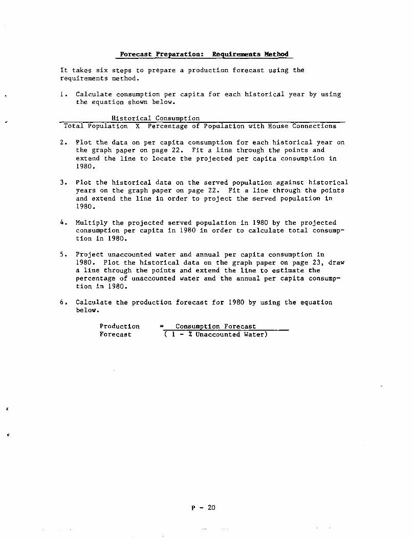
Forecast Preparation: Requirements Method

It takes six steps to prepare a production forecast using the requirements method.

1. Calculate consumption per capita for each historical year by using the equation shown below.

Historical Consumption Total Population X Percentage of Population with House Connections

2. Plot the data on per capita consumption for each historical year on the graph paper on page 22. Fit a line through the points and extend the line to locate the projected per capita consumption in 1980.

3. Plot the historical data on the served population against historical years on the graph paper on page 22. Fit a line through the points and extend the line in order to project the served population in 1980.

4. Multiply the projected served population in 1980 by the projected consumption per capita in 1980 in order to calculate total consumption in 1980.

5. Project unaccounted water and annual per capita consumption in 1980. Plot the historical data on the graph paper on page 23, draw a line through the points and extend the line to estimate the percentage of unaccounted water and the annual per capita consumption in 1980.

6. Calculate the production forecast for 1980 by using the equation below.

Production = Consumption Forecast Forecast ( 1 - X Unaccounted Water)

P - 20

INSTRUCTOR NOTES

Requirements Method (continued)

1. After the participants have prepared forecasts using all three methods, bring the group together to review them, beginning with the requirements method.

2. Ask a representative of each group to display the group's 1980 production and. consumption forecasts on the board or flipchart. Ask the groups to compare their forecasts and to discuss the reasons for any differences among them.

3. The calculations for the 1980 forecasts are shown below. (Because fitting a free hand line in order to project future data is imprecise, you can expect some variances among the group's calculations.)

H i s t o r i c a l Data

Tear

1961

1962

1963

1964

1965

1966

1967

Consumptl

76 KM

1.39 MM

78 MM 1.49 MM

87 MM

1.59 MM

100 MM 1.70 KM

96 MM

1.83 MM

91 MM

1.96 MM

116 MM

2.09 MM

on Per

0.68

0.67

0.68

0.70

0.69

0.68

0.68

Cap

•

•

-

-

•

•

-

lta Per Year

80 a 3

78 m 3

80 m3

84 a 3

76 . 3 .

68 a 3

82 a 3

Served Population

.94 MM

1.00 MM

1.08 MM

1.19 MM

1.26 MM

1.33 MM

• 1.42 MM

Projected Data ( froa graphs)

1980 Projected Consumption - 4.0 • 79 • 316 MMB 3

316 Projected Production - , ° ,, - 416 NMn3 J 1-0.24

Tear

1980

Consumption

by House

Connections

(In millions

• 3 per year

223

Production

(In Millions

m3 per year)

339

Actual Data

On-

Accounted

Water

34 Z

Total

Population

(Millions)

3.95

Population

with

Houae

Connections

90X

1-21


Use the space below for your calculations.

P - 21

INSTRUCTOR NOTES


4. The graph for projecting total'and served population is shown below. (Because fitting a free hand line in order to project data is imprecise, the participants' graphs may vary slightly.)

1 - 2 2


Plot the historical data and project future data for the total and served population on the graph paper below.

10

9

'fte tiz Feyncri't? s "Method

Total and Served Population

1960 62 64 66 68 IF 72

Years

. » 74

. .•

76 78 1980

P - 22

INSTRUCTOR NOTES


5. The graphs for the projected percentage of unaccounted water and the annual per capita consumption are shown below. (Because fitting a free hand line in order to project data is imprecise, the participants' graphs may vary slightly).

Percentage Unaccounted Water

30

20-

t Projected Unaccounted Water • 0.24

1960 62 64 — i 1 — — I 1 r -

66 68 70 72 74 Years —

-l 1 P 76 78 1980

Annual Per Capita Consumption, m^

80-•

70--

60"

V

h 19'6*0 62 64 66 -68 70 72 74 76 78 1980

Vears

Projected Annual Per Capita Consumption = 79tn3

I -23


Plot the historical data and project future data for the percentage of unaccounted water and the annual per capita consumption on the graph paper below.

3a

20

—r I960 62

jrclenta I "Per cl - T T —

' ! i » • T e Unaccounted Water

i r 64 66

—r 68

T 70

Years

72 \ I 74 76

"1 1 78 1980

Annual"Per "Capita Consumption, in

80-

70-

60-

I -i r

1960 62 64 -T" 66

—i r 68 70

— r -_72

Years

74 -i \ r 76 78 1980

P - 23

INSTRUCTOR NOTES

Exponential Method Time required: 30 minutes

1. Before participants begin work on the forecasts, review the instructions on page 24 for forecasting production using the exponential method.

.11

1 - 2 4

Exponential Method

Cakes four steps to prepare a forecast using the exponential method.

Plot historical consumption against each historical year or served population on the semilogarithmic graph paper on page 26.

Fit a line through the points on the graph paper and extend the line in order to project consumption in 1980.

Obtain the projection of unaccounted water in 1980 from the forecast you prepared using the requirements method.

Apply the projected consumption and percentage of unaccounted water to the equation below and calculate a final forecast.

Production = Consumption Forecast Forecast ( 1 - % Unaccounted Water)

P - 24

INSTRUCTOR NOTES

Exponential Method (continued) .

1. When you are ready to review the groups' forecasts using the exponential method, ask a representative of each group to display their 1980 forecasts on the board or flipchart. Ask the groups to compare their forecasts and to discuss the reasons for any differences among them.

1980 • Consumption fron high In Million B 3

280

Projected Data

Unaccounted Water, Z

241

Production In Million B 3

280 1-0.24 - 368

Tear

1980

Consumption by House Connections (In Millions B 3 per year

223

Actual

Production (In Millions m3 per year)

339

Data

Water Un-Accounted For

34 Z

Total Population (Millions)

3.95

Population with House Connections

90:

1 - 2 5

Exponential Method (continued)

Use the space below for your calculations.

P - 25

INSTRUCTOR NOTES


2. The graph for the exponential method is shown below. (Because fitting a free hand line in order to project data is imprecise, the participants' graphs may vary slightly.)

i

3

i

1

9

8

7

6

5

I

1

19

• — t — — - - • * . — t — - a

...:..-....-. - i - : " • ' : ' : : •

. • : : • : . : : . . : : : . •

: • ' : : ] . : .

. AwWMWI [ T ( i w i i w p * 4 r t w - - 4 * . M4 t T - 4 ' I - I W w 3

. i . ; ^ ! :i.ii • • ; : . : : : : :

. ;

• ' " : : ' : : \ : ' . ~ ' :

• • : : : • - :

;

r^C . "

jSf

J :-.

i0 frf *

• • *

i j>6 6

1

~:-".":••-•• r ~ .

:..': :~]::r:::~

. .. j . . . . .

- — - j 7 7 7 '

- : - - - , - •

: : . . : ; _ - • ; :

: ; : ;

. . . .

I 70 7

T»rtro

- ; : - • - - - - - . - " _ •

. : . - : • • : - : . : • • " • .

; \.\ .... .

..

^^

*?M . . . : . .

.i —....-

... .......... - : .r - v v -

.-. • • ; ~ -

: • - : ' ' :

• !

. . . . . r -:z.-.i::'r':—~i—

i""• ri~~ :i

1

; . . . . .

_=__..T4__._-i

T^-lrhT \\,\S > ^

T r m — - - •••.- •

--.: j^>.

L : : : i ! 1 : :

.

. _.. . . . . .

. " - J • i • • - . : . : .

-:-.., :..-r

_r; : ; . . . . , .;.:.: . ......

. . ' " ' • ; ; • • .

-.- --^:^~

> " "7B ~m

• • ' . : .

:

\

k ITOJJBCCM

> Con a imp t Ian

. : : • : : ; : : :

. . . . i .

1... 1 1 \ ; ..'. : • . :

..-...;... | ! . • i

: • I

/ j

/

1 i iD

i | .

1 - 2 6


Plot the historical data and project future data on the graph paper below.

:

4

2

2 . .

1 . . .

. 9 . .

8

7

6

5 j

L

<

*

.: • . . . • : . . . : : . . . . . : . . . : . _ . - . .-. j . v . : . . . . _ : : . • • . . : . : _ _ : _ . . : : . : : . : ; _ . : _ : . . ; - . _

:-- —•"_—::•-—:.:--: : :._: ~ : .. : Annual Consumption iri iMillioTis tn^ - j . - - — —

——.-::-_: :..:.::J ._:._-.-: ...:.:._.. ;..:_:_.;..: :.;::: :._:__!.:.i.-._r:...::-.:_j._,j. -;.:._;-J^J. .-::).::_-. :_:.

- ?":'i': "'-"i-"!-::- '•':•'•::: .Lvi^L: - • r : 7v7"~~ : ^ :~~ t : ~~-d~~ :T j73 -^>~" - : ~

• - • • j ! i

: 1 i

! 1 .

.... _ i

• • : - • ! 1 - - - - • • "

"'...".'11 _TT~__ '."ll'll'Z ~~ ~T~

i •

... .._

.

_ _

-i —

— ._—.

•

, i

1

I i : - :

• - - - - "

!

. . ...

1

.vEEiTi

1

. . - ^ i ; . - - ^ ^ : i i ^ . - 7 ^ . - - - ^ - - ^ — — ^ . - . i - - : — - - : : : . : - - : - — ; . T ^ = ;: _ : ; • - ; : Y ^ ^ — ^ ^ ^ = ^ — j - . - • - —

- . . : . - ; : • : . - ; • _ - . • = = • ; . . . . . / _ : _ ^ . . . . T _ : _ : _ : . . : _ . _ . : : ._ • . . j - : : ^ . ^ - z - r = j T - j i - ^ ^ . - ^ L = . - - . - . - . ^ ^ . ^ ^ . " - • • - I . j - ^ ^ v — ~ _ ^ i ^ . - ^ - ; ; ; . r _ - _

s;-.>5ss:'.i^LE5E2i:~.-:i:-^:.£.-;-î:-^:î---= :-.r ; - l — T _ ^ ^ - ^ . ^ X ^ ^ ^ _ ^ L ^ H . ^ ^ ; — - — : - -^-fî- - - -"-" : î^L^=i^^^-4^î_^^_

i_ _ : . . . . . - : : - T . - . _ _ : _ | - _ - - . _ - - - . . ; _ - . _ .___ | . - _ . . . - _ : _ - - . _ . - _ „ _ ; . : T i . _ _ . . _ . . - _ : ( • - • - • _ - - . . - ^ _ _ - r ~ _ —

- - - : J : J : : ; - - : . . J . . . ." - £ _ : : - • . : - . . : : : - • : . : : I . _ : _•.•-.-. . : . : : - . . - : • - - : . . - . . ! • • — . " : : . ; ; . — ' ~ ; . - . : - - . - - : } - - — • . - . - . —

" :;in^^-;i^::r-= l.'ip:-i::7:'?~.;'J "-H: --". .-I- "j ^^.r^r-^'y'T.if? -•- * j-

:..:....: - - _ : : _ . . " r \ . ^ _ " : . . - . • - - _ - } - _ - .

, j . . " : : . . . . . . I . . : . " . . z . . . — 1 .zr^rnrmT^r;

— : - • . - ; _ X 7 - _ = : - — :.j--—^r_v_ : - - := .^=rrJ_ . : i -"^

.- — -- - -- -. — — - : - • • : : — - - • . : : . ! r . : : :: ~

— — - : . - : . : . - . . : :z_..-.

r.-V.-i:. ••—-:'-=1^r:-'fI.f 1 —

.'. ; •_. ; • : ~T~~Zl'-2-zl

. : : . . . . . . . . . ::: : . - - \ \ z . - . : : : . - : . ~ z - . - : : _ . • ; — • - - — •• — « . . . j - . . . - . .

- - • • I • •• • - — • - t - i

1 - • T - r — ^ j -^ j i i

n

, \ --E='- • ^T"--'-=T — r» • • - -jn • — -th ' -ti ' - -i r -TO ^ n

>ftf> K? n<i n o u o I \ J i t ; H I \J / W >•-> * - : i

1 • - — — - i — — - - • • ! —

1 l e l i . 3

.

i n 3 U

fc— ^ — -

P - 26

INSTRUCTOR NOTES

Explanatory Method Time required: 30 minutes

1. Before participants begin work on the forecasts, review the instructions on page 27 for a forecast using the explanatory method.

1 - 2 7

Explanatory Method

It takes five steps to prepare a forecast using the explanatory method.

1. Plot the annual historical consumption against the number of house connections for each historical year on the double logarithmic graph paper on page 29.

2. Fit a straight line connecting the points of historical data, and extend the line.

3. Project the number of house connections in 1980 using the semilogarithmic paper on page 30. Plot historical data on house connections for each historical year, fit a line through the points and extend the line to project the house connections in 1980. In reality, the utility's planned number of house connections, according to investment plans, would be the basis for the connection forecast.

4. Record the projected number of house connections in 1980 on the graph paper on page 30 where you plotted historical consumption. Use it to read off the total consumption projected for 1980.

5. Obtain the projected levels of unaccounted water from the previous two forecasts you prepared and calculate the final forecast using the equation below.

Production = Consumption Forecast Forecast ( 1 - % Unaccounted Water)

P - 27

INSTRUCTOR NOTES

Explanatory Method (continued)

1. When you are ready to review the groups' forecasts using the explanatory method, ask a representative of each group to display the calculation of the final production forecast on the board or flipchart. Ask. the groups to compare their forecasts and to discuss the reasons for any differences among them.

2. According to the graphical forecasts, the number of house connections would be 440,000, the 1980 consumption would be 270 million m3 and the 1980 production would be 270 = 355 million m3.

1-0.24

3. The actual data for the period 1970 - 1980 are shown below.

Year

1970 1971

1972 1973 1974

1975 1976 1977

1978 1979 1980

Con

by

sumption

Rouse

Connections

(in mJ

HI 11Ions

per year

143 147 160 172 183 197 205 208 208 209 223

Production

(In •-»

Millions

per year)

191 196 216 246 253 253 265 286 299 314 339

1 - 2 8

Water

On* Nunber of

Accounted House

Por Connections

25* 251 26 X 30 X 28X 22X 231 27X 30 X 34 X 34 X

224,000

238,000

255,000 282,000 302,000 323,000 345,000

369,000 393,000 413,000 433,000

Population Total

Population

(Millions)

2.41

2.55 2.70 2.86 3.02 3.19 3.28 3.57

3.79 3.87

3.95

with

House

Connect

75X.

77X 78X 82 X 82 X 83X 84 X 85X 86 X 88 X 90 X


Use the space below for your notes or calculations.

P - 28

INSTRUCTOR NOTES


4. The graph for the projected annual consumption is shown below. (Because fitting a free hand line in order to project data is imprecise, the participants1 graphs may vary slightly.)

•) i b 7 «

^ „

1.

a

, 270

?

I

a

t-

4

3

]

, 3 4 i t

• • ! ! 1 :

• ,

t

1

J.; 1 1 : ! ( 1

i I i

M - : i ! 1 1

; ; ; ]

,.-.|-...J...,-J-.U i y

i U /ii i J\ : ! !

f \ • • 1 !

J f . 1 : i • y \ i i 1

J4 ; ! • 1 1 : ! 1

i i : : | :

'

n

! i ! 1 : i

• i :' i ' i ! I....:., i J ' j . L . j -! ! : i • ! ! 1 ! : j . • j - l

' " \ T"irr ! ; ; * i .

! . . . | .„. _L__j-l-

i : • ' ' 1 1

'i i i '

y|lB gJ i

1 1 ; 1 :

i : :

h i ! ' 1 !

1 ! ! i i : ! i

i i

h i 1 : : ! i ! 1 ^nn i 1 • i

Mi :

!

;

! '

!

>

:

1 :

1

•

"

1

1

; 1 ! : 1 1

•: 1

:

...... - • -

--

1 j : 1

! i :

! i

1- :

i

i 1

:

'

t

4 5 ^ 7 3 9

440 ' 2

Thousands of House Connections

3 4 b f> ' a «

1 - 2 9


Plot the historical data and project future data for annual consumption on the graph paper below.

1 Q

8

7

6

5

4

->

2

1 2 3 4 5 2 3 4 5 6 7 8 9

• -T r : :.;.; : : i : " : M : \:V:jzil\:: - ! ; ;;:i::: :!i ;:i::i::::! ; : ; i ; i H.i . :.j;.;:i;: N : : ! : - : ; . i ! v i - M : ; = ;! • • : : : ; : : i ; : : i : • • ! - - ; • • ! • 1 •; : - M - i M - - I -

: : . . ; : ; •

. . . .

: ^ l •::•: : \ :H •: I : i : i : : j . : .1 : ::j- 'i •' : : i 1 3 ! j : :r :^:.L::

Annual Consumption . i i i M i l l i o n s ns : . . . ; . . . : . . . ; : : : 1 : !....

: : : : • : : • : : : : • : ! : : : : : : : : : ; - ! : : : j : : : : : < : : : :

: : : : : : : j : - - - : i : - j • • • | • ' j , 1 ! :

• - • ! • • • ! • - • •

I • • : ; • • • • !

.........

: : ;;.i.i;:]h-;!:-;:i- :-:::; ;i : : : ! - — :;!;=!: : : - : : - - i i : : : : : : : i r - : i ; i : ; : . ; ! - -.. .. ..... : . . . .

! 1 . . 1

9.

8 -

7 .

6 .

5 .,

4

3

2

1

; - : - • - — • : - : : ^ - \ - : .

•~~~ -"-: - \i.xil-_i._

- - • • i - r ^ i l - ^ r i : ^ ^

i • • • • • • • {

I : : : ; : : - : : ; : : : : : : : : :

." — < ::::

m^-. • • ;• j j

; - "~n - -.-.''- : : : - • ! . , :. ' i r : :.-~::l\ '•": r !."

.._.

: :-: :iJ.EJ~.H::l=7IEf:'Enj - ^ — H

- • • - ^ - - ^ - : : - : | : ; ~ : ^ - # i -

:-: ~ iz:z:-

' • : ' • : 'r.::::-:'!•-: l r

~. '. . 1 ". '. .'1 ' '. *

f.__....... ,_.._-

M'iiMiiiHiiMi :.:U::f ^Li^îniliiit?!: ivitr^' • ^ : ; - . ; ; : : : : : ; i ; : ; ; i ; - h ? : | : : "

.. ...... ••::y.z:

T

.........

—,.... . . . . . .

1

hiiiz=

tm Hi . . . . j . . _ .

;. : : : • .

::::

::::

i:::

::::

....

liiii ;~

^

—

EE

. . . . : : : • • : . • . . :

- ! - • : ! - • • : 1

: . : : : • : : • . : : | •. :

:::: :::j :-::!:• 1 . . j

: : : • : : • : • : : : : ; : : : : : : " : r i : :

i-i ; ; • : - ; i i - ; - ! -

N T = ! - r i : . - J i : ^ l : -

mrr^m^

iij'iT^'fe-

îH3=; 1

.... i

! ^ ^ ^ . ~ - ^ ^ - ^ ~ J ; I : J :::.).. : =r

•_

. . E ^ _ - ^ ^ I

~.'Z'.

:

.Z.'ll'Z- ZSZZZ "-"_:

.........( _.. .. . . :::-:i:;::4:::^:--jiL--^::__-Li^_-;.z_::j_z-;

:::,i::.::l::::r:::; ..-.-.- .::•.: ; ::::-.•

••:-vrî"T^^:.::-a::^:;h;;M^M;H^:}i-

,:.v:-:-.-:-|,:::::^:::::::r-.::.: :.:::M ;;; .i^M":::

• • • ' —

• •

t • • • • -

. . . .

.;:::

H i M -h.......

T | -TT- -7 fT^=

:..

. . . . ] . .......,..J .. :.. . . ..

-Hi-: : f-. ! -

MiiMiii'i:

_:rzrp::

• • - - j i

! T

" — r r r

hzr-r-j '

---—.:. ::--, FÂ:-~:rr

=M^ . , ....

._._:_...

~ ^ ^ - ~

..... ...

•ii:;:::: • : : : • : : : :

: : : • • : : • •

iiiiiiM r •

v ••

! i

-j-— : ' . : • -

ii-HH==

.—.-rrrrfury

r '-

-----

-•"•LZ:

• - - : • •

- - . • • - : -

-—.--.-

•iiiiiiiii

. . . . .

: : : - •

:rJ:T

J~-: ;

Mriii

" - • - -

-----

' H i Z

. = = -

'ii

• : • :

• •

• : - " :

"ii

• ' - ' -

...

'zz

— 7.-

15

EE

f:

T:~T:£

........

# ;

—

"::

2 3 4 5 6 7 8 9

Thousands of House Connections

P - 29

INSTRUCTOR NOTES


5. The graph for projected house connections is shown below. (Because fitting a free hand line in order to project data is imprecise, the participants' graphs may vary slightly.)

Thousands of House Connect lone

Prnjprrcri

1960 62

Number of House Connections

- W.000

64 66 68 70 72 74 76 78 1980

1-30


Plot the historical data and project future data for house connections on the graph paper below.

. ..Thousands of House Connections .

-"•-•~-"~i :£Ii^:i;-1 .

9

s 7

6

G

4 .

3 . .

2 .

1 . . 19

i

" . JL '_'_

- -!

' Z L—L.—L "i

i

i i

: . ' _ : . _ : . : • ; j i - . • • . = . . • • . • • • . : \ • • = . . - . • : • . ; i : . : • • • • . - 1 : • • • • : ' . • : : - . : - ! • • ; . - - - . :

• • - ' : ; : : • : - ; -.-^ : - ; . = - i - - • ; j - : - : : . - .

. . : • • • " . • . • ; . . ' • ' ; . ; • . • . : . : • - I - . - . : . - ; - " . - . 7 : _ : • • - • - ; • : - — . . ; • : : . . • . _ . - . . • . . : . • • • . - - - . - -

. : • : ; • - . . r • . . - . - • . . . •• • • . . ' ; . . : . ' _ - • ~ ^ : ^ ? ^ : ; - : - : . L : ~ H . : . : : . ' " " : : ~ ; - : . i - : : i L : : . • - ; • : • • - > : • : . .

. ' _ : ' . . . ' ; . _ . ! " ' . : • ! ' " . . . . : • i ..'... • 1 :.:Ci"":J±.'.- , . • : . - . : " . . . . . . . _ _ _ . : : : . _ ; _ : . :

. . . _ . . ; - j •: i ; ; - - r • :- • • ; ; - : ; : • - • - - H - ' T " - - : - - ^ " ^ ^ . - ^ : ~ - : ^ ; - 7 : - ~ ^ - { ^ L ; = - -

T^----T-::- ; : - :r^f7- . -T-i7H^ : r l - : - - ; - ; -h~-~-:-- i - : :v: •—'• • • ; . - -" . :T~}\. '.'".. ' •-'.~'-iiizrz-"'.'. - " : - : - "• • " J -

; ~ -::-:•:-.•: -.:-.-.:• ; ::r. : - : _ : : . _ - : . : - v: - - | .•: .. .-. ;•-:.::.:: - i ..... - : : . = - - - — - . : . - - . I • :_-_--_-=—.—: • v —:• , - - — : : : z

.'--.'-' :-\—.- Z-]l---:i:Z-—-=}~-:r-r~:'::l ' :'—~:'-:1:: " ~~^~7 "rf^.™:: -IrJiivT^':-:1^^1^-.1"^^ .-"T_~ -~r-^^z

; • • - ~ — ; — • - ! • - 1

- - : • - - • - - • • > - - ; •

t - --- : —J- • • - |

. . 1 — . 1 — . ; . — ,

- - 1

: . . ~-~—Z.:.. .___ ~~~s : J i

| 1

. . ....

i

• - ! ; • • • • ! • - - - :

! I

-:r^:LU..^ziz_—_::_. :r• T_;^: ;

i

. 1 i

. .

.

1

l i

, i

i

i

1

i

jr^::-._ti

L i ! ;

- •:

•

•

: " " - - • — — - - - - -

. . .

_. ..._. __ :._ 1

" " |

60 62 64 66 68 70 72 74 76 78 1980 Years

P - 30

INSTRUCTOR NOTES

Analysis and Comparison of Methods Time required: 20 minutes

1. After you have reviewed the three forecasts that the participants prepared, assist them to compare the methods against the criteria listed on page 31. The participants should recognize that each of the methods may be more appropriate under certain circumstances or with certain projects.

2. Conclude the activity by assisting the participants to plan how they can use the information on forecasting methods for the projects with which they work. Ask them to identify any obstacles to accurate data collection and forecasting so that you can help them identify solutions or alternatives.

1 - 3 1

Analysis of Forecasting Methods

Now that you have had an opportunity to use all three forecasting methods, discuss them with the other members of your group. Analyze and compare the three methods using the criteria listed below.

Ease or Difficulty

• Availability of Data

• Accuracy

Inclusion of Important Determinants

Reliability in Long-Term Forecasts

• Based upon Controllable Factors

P - 31

INSTRUCTOR NOTES

Conclusion Time required: 10 minutes

1. Summarize the content covered in the module and assist the participants to identify ways that they can apply the techniques of demand forecasting to the projects with which they work.

2. Point out that the next pages include copies of the visuals and narrative text from the slide/tape program.

1 - 3 2

DEMAND FORECASTING

SLIDE/TAPE PROGRAM VISUALS AND NARRATION

•a

P - 32

a

»

IP

DF-1

DEMAND FORECASTING - PART I

TITLE SLIDE: Demand Forecasting

Part I

NARRATOR:

Development projects, like these,

are often undertaken in order to

satisfy present and future

demand. In the case of these

projects, the objective is to meet

the community's demand for

safe water.

Demand forecasting is the

technique used to estimate a

community's future needs. Those

needs, in turn, are the basis for

deciding which projects are

necessary and when they should

occur.

The terra demand describes the

quantity of water that the

community wants for consumption.

Because demand and consumption are

often synonymous, when we discuss

how to forecast demand in

this program, we will mean how to

forecast consumption.

The term supply describes the

production levels that will be

necessary in order to meet future

consumption. Supply forecasts,

therefore, are based on

consumption forecasts.

Demand forecasting is important to

the economic justification of

projects. Overestimated demand

leads to projects that are

unnecessarily large and waste

scarce resources, including land,

labor and capital. Underestimated

demand results in undersized

projects that fail to meet demand.

DF-3

7. Second, accurate demand forecasts

are important to the technical

justification of projects.

Inaccurate forecasts can lead to

projects that are sized and timed

incorrectly. As a result, those

projects do not represent the

least cost solution to meeting the

community's needs. And they are

too complex or limited to produce

the intended benefits.

8. Third, accurate forecasts are

important to the financial

justification of projects.

Overestimated demand leads to

overly optimistic revenue

projections. In this case,

financial crises result when

projects must be paid for despite

the inadequate levels of revenue.

9.

•'• • Characteristics of Demand ;

.V.'.'8 Determinant* of Demand -.-

P'~.9 Forecasting MeU»od»4-".--.,rl '

In this program, we will review

the three elements to consider

when forecasting demand. They

are: the characteristics of

demand, the determinants of

demand, and forecasting methods.

DF-4

10. First, the characteristics of

demand. We will review the

different types of demand, how

demand is measured and how

consumption is distributed among

the people in a community.

11. Second, we will identify the major

determinants of demand. Deter

minants include the price of

water, the extent of metering, the

consumers' income and the service

level provided.

12 And, third, we will examine how to

prepare forecasts using three

methods: the requirements

methods, the exponential method

and the explanatory method.

13 Now we will turn our attention to

the first element, the character

istics of demand. We will begin

with the types of demand found in

most communities.

One type is domestic demand for

water to be consumed at home.

Another type is demand for water

from the commercial sector...which

can be significant, particularly,

in service-oriented cities.

The industrial sector also has de

mands for treated water. In some

cases, large industries may even

require their own water supply.

And, the public sector, including

government buildings, hospitals

and schools, represents yet

another type of demand.

Next, we will review how demand is

measured. One way to measure

demand is to identify the quantity

of water that the community

consumes during a specific period

of time. Water consumption can be

measured in thousands of cubic

meters per day, in millions of

gallons per day, or in liters per

second.

Another way to measure demand is

in liters per capita per day based

on the number of people who have

access to piped water. For

example, a community's consumption

level may be 250 liters per capita

per day, including domestic,

commercial, industrial and public

sector consumption.

DF-7

20 Usually, a community's demand is

expressed in terms of average

daily demand levels. Average

daily demand is calculated by

dividing total annual consumption

by the 365 days of the year.

21 Average daily demand can be

plotted on a chart such as this

one. The vertical axis represents

demand, and the horizontal axis

shows time. When demand is

plotted for a number of years, the

result is the community's average

daily demand curve.

22,

•."_ Variations im.'-;-:.V: Average Daily Demand^ • Seasonal Taraparatam.."' .

• Water U u Hablt*.-^- S->-

Two factors contribute to

variations in average daily

demand: seasonal temperatures and

water use habits. During the

hottest seasons, consumption of

water will increase. The

population's water use habits

during certain days of the week

may also affect demand. For

example, more water may be

required on the days when clothes

are typically washed.

DF-8

23. Daily variations in demand can be

calculated as a percentage of the

daily average demand. One varia

tion is termed maximum daily

demand. It describes the level of

consumption on the day of the year

when consumption is the highest.

It is often set at 120% of average

daily demand, but the precise

percentage will depend on the size

of the community and the climate

conditions.

24 This chart shows maximum daily

demand in relation to average

daily demand. Maximum daily

demand is parallel to average

daily' demand over time, at a level

20% above average daily demand.

25 A second daily variation is

described as peak hour demand.

Consumption varies during the 24

hours of the day, as shown on this

chart. Demand peaks in the

morning and in the early evening

hours when consumption is the

highest. Demand is lowest during

the night hours when the least

water is consumed.

Peak hour demand is substantially

higher than both average daily

demand and maximum daily demand.

Usually, it is set at 180% of

average daily demand. The actual

peak hour rate will be higher for

smaller communities and lower for

larger communities.

Here, peak hour demand is plotted

on a chart with average daily

demand and maximum daily demand.

The line representing peak hour

demand is parallel with the

others, but at a level 80% higher

than average daily demand.

In conclusion, demand levels can

be measured and expressed as

percentages of the community's

average daily consumption. 0

cubic meters a day represents

average daily demand. Maximum

daily demand in this case is 1.2

times average daily demand, or

1.20 cubic meters per day. And,

peak hour demand is 1.80, or 1.8

times average daily demand.

Next, we will turn our attention

to supply. Supply is the

production level needed to satisfy

demand, or consumption. Supply

can be plotted along with demand

on a chart such as this one.

The levels of production and

consumption discussed so far are

the levels that are accounted for,

or measured, in some way, such as

metering.

The difference between metered

production and actual consumption

is termed unaccounted water. It

is the amount of water that is

supplied but does not generate any

revenue or is not measured through

metering.

In this case, the unaccounted

water is the highlighted area on

the chart. Like supply and

demand, unaccounted water can also

be described in thousands of cubic

meters per day.

It is important to add an amount

for unaccounted water to

consumption forecasts in order to

prepare forecasts that accurately

reflect the required supply.

Usually, unaccounted water is

expressed as a percentage of the

amount of water that is produced.

In order to calculate unaccounted

water, first consumption is

subtracted from production. Then,

the remainder is divided by

production.

v" *" * '_ Unaccounte : CefasunpHon^' -. Water.:.:

This chart shows the water

production that is required with

different percentages of

unaccounted water. Q represents

the consumption level. If

unaccounted water is at 67%, then

the chart shows that the water

produced must be triple the amount

of water that is consumed,

represented by 30 on the chart.

A 50% level of unaccounted water

requires production that is double

the level of consumption,

expressed as 2Q. As this chart

shows, the production levels

required decrease if the

percentage of unaccounted water

decreases.

The level of unaccounted water is

one indicator of the efficiency of

a water supply system. It is

important, therefore, to keep the

percentage of unaccounted water as

low as possible. A high level of

unaccounted water signals that

more consumption could be

satisfied with existing water

production levels. An efficient

system is one where unaccounted

water is 20% or less.

Next, we will review some causes

of unaccounted water. Leakage is

one cause. A portion of the water

produced is lost because of leaks

in the distribution system. The

actual amount lost will depend

upon the age and condition of the

pipe as well as the condition of

the surrounding soil.

Some more water will be consumed

through unknown or illegal

connections to the distribution

system. These connections are

unmetered and, therefore, the

water consumed is unaccounted.

A third source of unaccounted

water is known, but unmetered

connections. In some cases,

communities meter very few

connections. In other cases, the

community may not meter certain

facilities, such as schools,

hospitals, and government

buildings, because they are exempt

from paying tariffs.

A fourth cause of unaccounted

water comprises the meters that

underregister the actual amounts

of water consumed.

And, fifth, faulty production

meters may overregister the amount

of water that was produced. This

will make unaccounted water seem

higher than is actually the case.

Of all the causes of unaccounted

water, typically, leakage is the

least important.

It is common for the percentage of

total unaccounted water to amount

to 30% of total water produced.

In the best managed and most

efficient facilities, the

percentage of total unaccounted

water amounts to only 10% of the

total water produced.

The third characteristic of demand

that we will discuss is the dis

tribution of demand in the

community.

Metering data is a source of

information for compiling

statistics on the distribution of

consumption in a community. In

this statistical table, all of the

house connections in the community

are divided into deciles, that is,

increments of 10%. Each decile is

listed in ascending order of its

consumption level.

Then, a relative share of the

total water consumed in the

community is assigned to each

decile.

This chart shows that the 10%

decile, the group with the lowest

consumption, consumes only 3% of

all water supplied. The 90 to

100% decile, the group with the

highest consumption, accounts for

35% of all water consumed. In

terms of average consumption, the

90 to 100% decile consumes 10

times more water than the 10%

decile.

Another way to show the distribu

tion of consumption in a community

is a bar chart. This one shows

each decile's share of total

metered consumption. Low income,

domestic consumers use relatively

very little water. Industrial and

high income domestic consumers

account for significantly higher

consumption.

This chart shows the cumulative

share of connections in ascending

order of consumption.

Then, each cumulative share of

connections is shown next to its

share of total water consumption.

In this case, the group that

represents 40% of all house con

nections in the community consumes

only 13% of the total water. Most

likely, these are low-income,

domestic consumers.

A summary chart, such as this one,

is useful for showing the cumula

tive percentage of house connec

tions for each group and its

corresponding cumulative percent

age of consumption.

These distribution figures are

valuable when forecasting demand.

Among other things, the figures

show that adding house connections

will have a different impact on

consumption, depending upon which

consumer groups are connected. On

the one hand, connecting more low-

income households will have a

minimal impact upon total water

consumption. On the other hand,

increased connections for high-

consuming groups will have a much

greater impact upon consumption.

In summary, demand forecasting

first requires an understanding of

the characteristics of demand.

Specifically, the characteristics

of demand involve understanding

the different types of demand, how

demand is measured and how con

sumption is distributed in the

commmunity.

This concludes the first part of

the program on demand forecasting.

(End of Part 1)

DEMAND FORECASTING - PART II

Title slide: Demand Forecasting

Part II

In this part of the program, we

will discuss the determinants of

demand, beginning with price and

metering.

The price of water is equal to the

tariffs that are charged for it.

Price is usually expressed as an

average tariff per cubic meter of

water consumed. The average

tariff is calculated by dividing

the total sales revenue by total

metered consumption.

DF-20

58 The price of water influences

consumption levels only when

consumption is metered. Because

metering is so closely linked with

price, the two will be discussed

together in this part of the

program. B

59,

jUfighi Price:-rr: High Beneflta£&$£:

3VLow Price:'--T:tow'Benaflts?^-?:-'

The price that consumers will pay

for certain amounts of water

reflects their perception of the

benefits they receive from that

water. Consumers will pay a high

price for water that provides them

with a high level of benefits.

They will pay less for water that

they believe provides them with

fewer direct benefits.

60 This demand curve shows that the

price that consumers will pay for

water reflects the benefits they

perceive they are getting.

Consumers will pay a high price

for water that provides a high

level of benefits. As the arrow

indicates, consumers will pay less

for water that provides fewer

benefits. Next, we will examine

some reasons for the differences

in benefits perceived and the

prices that consumers will pay.

If the consumer is without any

water, his need for it in order to

survive will be acute. He will

pay a very high price for this

critical amount of water because

he perceives the benefits of this

amount of water to be equally

high. The consumer may also need

additional water for food

preparation. This is important,

but less vital, so the consumer

will pay somewhat less for this

amount of water.

The consumer will pay even lower

prices for additional amounts of

water for hygiene. And, he will

pay the lowest prices for other,

non-critical uses of water. This

demand curve, then, shows the

decreasing prices that consumers

will pay based upon the value they

place on each amount of water.

The shaded area under the demand

curve represents the total econo

mic benefits perceived by the

average consumer.

In addition to an individual con

sumer's demand curve, it is also

possible to depict a community's

demand curve as well. A com

munity's demand curve will show

the same trends. This is because

a community also will pay accord

ing to the benefits that the water

provides.

Price changes, however, can affect

demand, both in the long and short

term. To illustrate this point,

we will use the example of an

individual who is consuming a

quantity of water represented by

0 0 on this chart. For that amount

of water, the individual consumer

is paying a price represented by

V

If the price is increased from Pn

to P , the individual will

consume less water. As a result,

the quantity of water he consumes

each day will decrease, from Qn

to Q .

DF-23

67 Price elasticity is the indicator

used to measure how much demand

will increase or decrease if

prices rise or fall. Price elas

ticity is calculated by dividing

the relative change in water con

sumption by the relative change in

price. That calculation requires

three steps.

68 The first step is to calculate the

average price and average

quantity. In these equations, 0

represents the quantity of water

consumed and P represents the

price paid for the water. The

average quantity is obtained by

dividing QQ plus Q, by 2. The

average price is obtained by

dividing P_ plus P, by 2.

69 The second step is to calculate

the average relative changes in

both quantity consumed and price

paid. The relative change in

quantity is calculated by

subtracting Q1 from Qn. The

relative change in price is

obtained by subtracting P. from

PQ. The average relative change

is then calculated by dividing the

changes by the averages.

The third step is to calculate the

price elasticity by dividing the

relative change in quantity by the

relative change in price.

Studies have shown that, in the

short-term, price elasticity of

water demand is approximately

minus 0.3. This means that con

sumption will decrease an average

of 30% if the tariff increases by

100%.

Studies have also shown that the

price elasticity for low-income

consumers is lower, almost zero.

This means that consumption levels

for this group will remain almost

constant "regardless of any price

changes. The reason is that this

group primarily consumes critical

water that provides them with a

very high level of benefits.

In contrast, the price elasticity

for high-income consumers is

higher. It is estimated at minus

0.6. The demand curve is not as

steep because this group consumes

more noncritical water. As a

result, if prices increase, this

group will tend to decrease its

consumption of non-critical water.

Because price changes do influence

consumption, it is possible to use

price changes to control the com

munity's demand. For example, if

annual demand is increasing so

fast that rationing may soon

become necessary, a tariff

increase can be used to curb

demand. When the tariff increase

reduces demand, then the community

will gain some additional time

before it must increase

production.

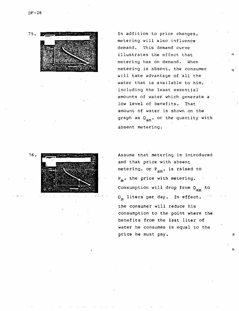
In addition to price changes,

metering will also influence

demand. This demand curve

illustrates the effect that

metering has on demand. When

metering is absent, the consumer

will take advantage of all the

water that is available to him,

including the least essential

amounts of water which generate a

low level of benefits. That

amount of water is shown on the

graph as 0 , or the quantity with J am

absent metering.

Assume that metering is introduced

and that price with absent

metering, or P , is raised to a am

P , the price with metering, m c 3

Consumption will drop from 0 to am

0 liters"per day. In effect, m u

the consumer will reduce his

consumption to the point where the

benefits from the last liter of

water he consumes is equal to the

price he must pay.

Studies have shown that metering

will cause per capita water con

sumption to decrease approximately

40%. This means that metered

consumption is approximately 60%

of unmetered consumption.

Because metering can decrease

consumption, it is useful in

controlling demand. And, when

demand decreases as a result of

metering, the community will gain

some additional time before having

to increase water production.

This chart shows the cumulative

share of consumption by different

groups. When metering is

introduced, it is best to begin

with the higher income consumers

and work gradually toward metering

the lower-consuming groups.

This concludes the second part of


(End of Part II)

DEMAND FORECASTING - PART III

Title Slide: Demand Forecasting

Part III

In this part of the program we

will continue to review the

determinants of demand. Now that

we have discussed price and

metering, we will turn our

attention to income.

Income levels influence

consumption. This relationship

can be shown on a graph where the

consumer's income in dollars per

month is plotted against his

consumption in liters per day.

As this curve shows, water

consumption increases when

consumers have more income per

month. Higher income increases

consumption for two reasons.

First, more money is available to

pay for consumption. And, second,

consumers can afford more

water-using appliances and

sanitation facilities.

The relative share of the dif

ferent uses that consumers make of

water illustrates the importance

they place on increasing amounts

of water. The most basic need is

water for drinking and cooking.

Almost 10% of all water consumed

goes to this critical use.

Next, consumers need water for

personal hygiene. Approximately

30% of water consumed is used for

hygiene.

Dishwashing is another use of

water, and amounts to

approximately 10% of total water

consumed.

Using water to do laundry consumes

another 10%.

Gardening or non-critical uses of

water, such as washing cars,

requires another 10%.

Then, too, water is required to

operate the sewerage system,

amounting to about 30% of total

water consumption. The relative

shares on the chart are represen

tative of water consumption in

Western Europe.

The basic water needed for drink

ing, cooking, and perhaps hygiene,

averages 15 liters per capita per

day for a low-income population.

The water consumption for a high

income population is over

150 liters per capita per day.

Water consumption changes when in

come changes. Income elasticity

is the term used to describe how

much consumption will change when

income levels increase or decrea

se. Studies have estimated

income elasticity at 0.3. This

means .that when income doubles,

water consumption increases by

30%.

In addition to price, metering,

and income, the fourth determinant

of demand is the service level.

It can have a significant impact

upon the demand for water.

For instance, a community with

public standpipes consumes

approximately 20 liters per capita

per day. The time and physical

labor required to obtain

additional water discourages

consumption from rising much above

this level.

Households with yard connections

consume between 50 and 100 liters

per capita per day. Water use by

this group is higher because the

water is more accessible.

Consumers with house connections

or indoor plumbing consume even

more water — 100 or more liters

per capita per day. As this chart

shows, consumption increases as

the service level improves.

In addition to the four major

determinants of demand—price,

metering, income and service

level—there are other factors to

consider as well. These include

drainage, the continuity of

service, the service pressure and

the climate.

First, drainage. The absence of

good water drainage will limit the

amount of water that consumers

use, unless drainage by gravity is

possible. Consumers will decrease

their water use to the point where

the soil can absorb the

wastewater.

Continuity of service is another

factor to consider. Most

utilities aim to provide water

service 24 hours a day. If this

is not ' feasible, then water is

often rationed. But, in many

cases, rationing does not

discourage water consumption. In

fact, it may increase

consumption. This is because

consumers will collect water to

keep on hand while water service

is interrupted. Then, when water

service resumes, they may discard

the stored water and wastefully

replace it with fresh water.

Service pressure should be taken

into account because it, too, in

fluences water consumption. Water

consumption increases when service

pressure is high and water comes

out of the tap at a high velocity.

Last, the local climate must be

considered as well. On the one

hand, water consumption will

increase when the temperature is

the highest, most often during the

dry seasons. On the other hand,

consumption will decrease during

the rainy seasons when water is

more abundant and alternative

sources are available.

In summary, the level of demand

for water is determined by a num

ber of factors. The most influen

tial factors are the price of

water, the extent of metering, the

consumers' income and the water

service level.

DF-36

104.

The other factors to consider are:

drainage, continuity of service,

service pressure and local

climate. &•

This concludes the third part of


(End of Part III)

a

DF-37

DEMAND FORECASTING - PART IV

105 . T i t l e S l i d e : Demand F o r e c a s t i n g

P a r t IV

106. In this part of the program, we

will review how to forecast

demand using three methods.

107. FORECASTING METHODS

v?:~;'„'. .Future C6nsumptibij\ ;4~, Unaccpunted.Wateiri1:

' s r ' Future Production^::

Regardless of the forecasting

method used, there are three

important variables to consider:

the amount water that will be

consumed in the future, the amount

of unaccounted water and the

amount of water that must be

produced in order to meet

consumption and unaccounted water

levels. In effect, the future

supply - or production -

requirements are equal to future

consumption plus unaccounted

water.

When forecasting future demand, it

is useful to consider forecasts at

different points in time. This

chart is a short-term forecast.

It extends two years into the

future.

This medium-term forecast is tar

geted at years 0 through 8.

And, this long-term forecast

covers years 0 through year 20.

Forecasts that extend much beyond

twenty years are of little value

because the margin of error typi

cally is very high.

The forecasts prepared for

different periods of time can

influence the economic, financial

and technical justification of

projects. For example, errors in

short-term forecasts may affect a

project's economic justification.

This is because overestimated

short-term demand will result in

premature projects and an

unnecessary financial drain.

Similarly, errors in medium-term

forecasts will endanger a proj

ect's technical justification. On

the one hand, overestimated demand

will result in premature or over

sized projects where resources

will remain idle. On the other

hand, underestimated demand will

result in projects that cannot

meet demand.

Errors in long-term forecasts are

somewhat less serious. In this

case, there is time to remedy

under- or overestimated demand.

Because of the margin of error in

forecasts that extend this far

into the future, long-term

investment planning should be

flexible.

DF-40

114. Forecasting future consumption

begins with a base of historical

data on past consumption levels,

the percentage of unaccounted

water, the total population, the

population served and the number

of house connections.

115. It is also important to consider

any expected changes in the price

of water, the extent of metering

of connections and the consumers'

incomes.

116. Forecasting consumption requires"

predicting the future by using

historical data. We will use this

graph to illustrate how to plot

historical data and how to find

the curve that will best represent

future consumption.

One way to show future trends is

to plot the points of historical

data on a graph and then draw a

line, free-hand, through the

points.

A second way to plot the curve is

to use the least squares method.

First, the distances between the

points and the curve are squared

and added. The line is drawn so

that the sum of the distances from

each point to the line is the

least.

Then, the line is calculated using

the equation: Y equals a plus b

times x.

DF-42

120. Y is the annual consumption. X

represents time in years.

121. A is a constant. It is the con

sumption level in year 0 and is

the point where the straight line

intersects the Y axis.

122. And, b is the slope of the

straight line. It describes how

much the line will rise each

year. Fitting a straight line-—

using the free-hand method or the

least squares method is the

basis for approximating historical

data. The approximated historical

data, in turn, are important when

using any of the three forecasting

methods that we will review next.

123. The th ree fo recas t ing methods a r e :

the requirements method, the

exponen t ia l method, and the

exp lana tory method.

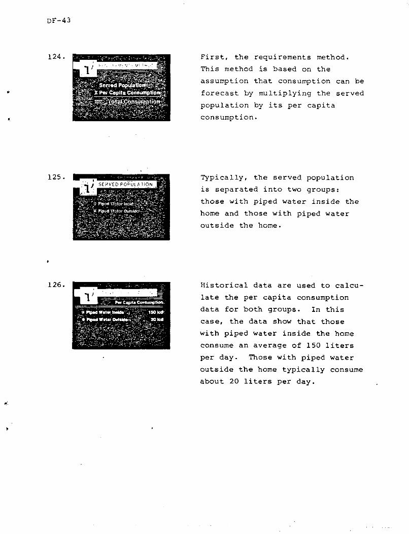
DF-43

124. First, the requirements method.

This method is based on the

assumption that consumption can be

forecast by multiplying the served

population by its per capita

consumption.

125. Typically, the served population

is separated into two groups:

those with piped water inside the

home and those with piped water

outside the home.

126, Historical data are used to calcu

late the per capita consumption

data for both groups. In this

case, the data show that those

with piped water inside the home

consume an average of 150 liters

per day. Those with piped water

outside the home typically consume

about 20 liters per day.

After historical data on the per

capita consumption of both groups

are prepared, population forecasts

can be prepared. Separate

forecasts are prepared for the

future population that will have

piped water inside and the

population that will have piped

water outside. On this chart, the

solid line shows past population

data; the broken line depicts

estimates of future population

numbers.

In addition to population

forecasts, per capita consumption

can also be projected for both

groups. Metering and price

changes should be taken into

account when preparing this- data.

In this case, the chart shows that

per capita consumption for those

with piped water outside will

remain relatively constant while

the consumption by those with

piped water inside the home will

increase slightly over time.

DF-45

129 In order to forecast total future

consumption, the information on

both population and per capita

consumption is combined.

130 This forecast shows that the popu

lation of 200,000 with piped water

inside has a per capita consump

tion of 160 liters per day. This

group, then, is expected to

require 32,000 cubic meters per

day. The second group is the

population of 10,000 with piped

water outside. It is expected

that this group will consume 20

liters per capita per day,

totaling 200 cubic meters per

day. When the consumption

projections for both groups are

added, the result is a total

consumption requirement of 32,200

cubic meters per day.

After the consumption forecast is

prepared, the next step is to

forecast the supply that will be

required to meet consumption. In

order to forecast supply, the con

sumption forecast is divided by

one minus the share of unaccounted

water (excluding standpipe con

sumption). In this example, the

consumption forecast was 32,200

cubic meters per day and

unaccounted water was estimated at

33 percent. The total supply

forecast, then, is 48,000 cubic

meters per day.

The primary advantage of using the

requirements method to forecast

demand is its simplicity. It is

easy to use and to understand;

therefore, it is widely used.

Caution should be exercised when

using the requirements method. It

is based on population data and

these numbers are often artifi

cially inflated. This can lead to

overestimated demand.

DF-47

134 In addition, caution should be

exercised because this method is

also based on per capita

consumption. These data are

frequently inflated in forecasts.

135

., Slmpncilp^^vc^-.-'V'^rt'.; -.;

;"'CautloissX:".:'] "'y- '''-'••

?; 9. (nHolod Po? Cflpifo Co«5umpU6«?'-

And third, population and per

capita data are largely external

variables that the utility cannot

influence. This is particularly

true with population figures that

are also the roost difficult to

estimate exactly.

136 The second forecasting method we

will review is the exponential

method. The exponential method

assumes that water consumption, Y,

is an exponential function of the

served population, represented by

X. D and F are constants.

137

= D LogY:'.;=' LogO +•FX

In order to construct a demand

curve, using the exponential

method, the first step is to take

the logarithm of both sides. The

result is the equation log Y

equals log D plus F times X.

Then, water consumption, or Y, is

plotted against the served popula

tion, X. On semilogarithmic

paper, the result is a straight

line like this one.

The next step is to project what

the served population will number

by a certain year.

Projected consumption then is

estimated by inferring future

consumption levels from the

historical data.

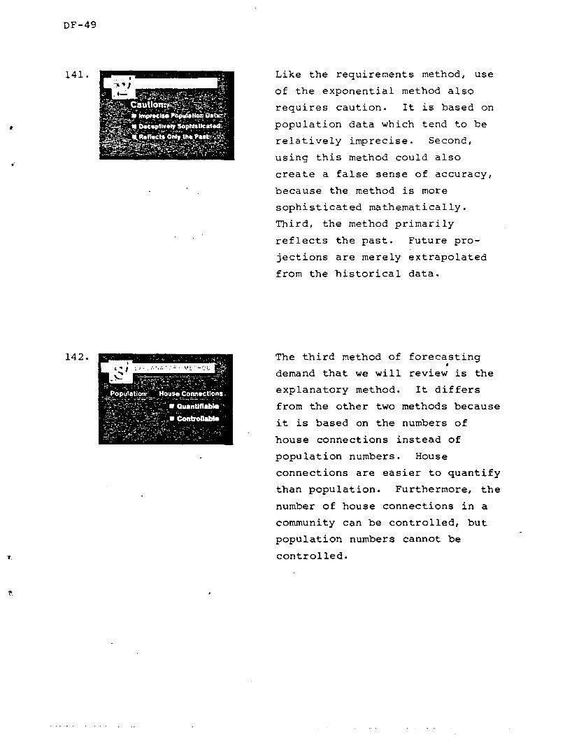
DF-49

141

^n' - ,4r . :-.^;-""..-- :".---•-*..*/-•"-''.- ~ -*: ^ S^.',..«.D»c»ptl»»tr Sophtollcattt r;

Like the requirements method, use

of the exponential method also

requires caution. It is based on

population data which tend to be

relatively imprecise. Second,

using this method could also

create a false sense of accuracy,

because the method is more

sophisticated mathematically.

Third, the method primarily

reflects the past. Future pro

jections are merely extrapolated

from the historical data.

142.

^Populations__[ House Connections.

'S-i'0^'^'-y'''m Quantifiable' ^ v - " . - . - . : & i V . ; i v - ^ > . L-.. . • . • • •-;.:'.x-.--.,:--.i-.^- ._• ControOabte "

The third method of forecasting

demand that we will review is the

explanatory method. It differs

from the other two methods because

it is based on the numbers of

house connections instead of

population numbers. House

connections are easier to quantify

than population. Furthermore, the

number of house connections in a

community can be controlled, but

population numbers cannot be

controlled.

The explanatory method assumes

that water consumption is a power

function of the number of house

connections. Y is the water

consumption, X is the number of

house connections and G and H are

constants. In order to construct

a demand curve using the

explanatory method, first, we take

the logarithm of.both sides. The

resulting equation is Log Y equals

Log G plus H times Log X.

Consumption is plotted on the Y

axis and numbers of house

connections are plotted on the X

axis. Then both variables are

plotted in logarithmic scale.

After plotting historical data on

consumption and the number of

connections, a straight line is

drawn connecting the points.

Next, the number of projected

house connections is calculated

for every year that will be

included in the projection.

DF-51

146. Last, projected consumption levels

are calculated using the points on

the line for the projected number

of connections.

147. The explanatory method offers

three advantages. First, it is

based on numbers of house connec

tions, which are easy to quan

tify. Second, the utility can

determine the number of house con

nections and control them more

easily than it can control popula

tion numbers. And third, this

method takes into account the fact

that average consumption per house

connection decreases as the

number of house connections

increases.

148. There are several reasons why

average consumption per connection

decreases as connection coverage

increases. The first households

connected tend to be in the high

income group. Unconnected

households often draw water from

those with connections. This

increases average consumption.

Later, when more low income house

holds are finally connected, the

number of connections is higher.

At the same time, the average con

sumption per connection will

decrease.

Regardless of which of the three

projection methods is used, it is

important to apply sensitivity

analysis to the results. Sensi

tivity analysis is a technique to

test what will happen if there are

changes to the assumptions on

which forecasts are based. Three

important areas to apply sensitiv

ity analysis are population num

bers, numbers of house connections

and per capita consumption.

For instance, actual numbers of

the population served may deviate

from assumed levels by 30%. Or,

the number of house connections

could vary 10% from estimated num

bers. In addition, per capita

consumption could actually be 20%

higher'or lower than the estimates

report. Any of these variances

could affect the accuracy of

forecasts.

DF-53

152. Because the assumptions on which

forecasts are based may change, it

is best to prepare a range of

forecasts. This will help to make

the final forecast as accurate as

possible. More accurate forecasts

will also help in planning project

investments and financing more

realistically.

153. There are three groups whose

demand or consumption should be

projected separately from the

population with connections. They

are industries, the unconnected

population and the rural

population.

154.

B Business Growths- '•;-?_.

. a Recirculation of Water

tt Alternative Water Sources-

Industrial demand is usually pro

jected on a case by case basis.

Very larye industrial consumers

are few in number but account for

a great share of total consump

tion. Where possible, projections

of their demand should take into

account expected business growth,

possibilities for water recircula

tion and potential reliance on

alternative water sources.

DF-54

155 The consumption of a second group,

the unconnected population, is

also projected separately, usually

using the requirements method. In

this case, population numbers are

multiplied by per capita consump

tion. The result is typically an

adjustment to.the forecast of

approximately 20 liters per day.

l'J»

156 The third group to forecast

separately is the rural

population, including the

centralized village population and

the dispersed population. These

groups' consumption is usually

projected using the requirements

method. In some rural areas, each

head of cattle consumes double the

amount each person consumes,

approximately 40 liters per capita

per day. In this case, the

consumption by cattle would be

added to forecasts of human

consumption.

157. In summary, these three forecast

ing methods take into account

several important variables that

influence future water supply

requirements.

DF-55

158.

.^'r?':>' l^y'fiire Cbnsiirnptioit ^ 1 4 ^ ' Urract^unffed Wa\er :

The variables include the

estimates of future consumption

based on current and historical

data plus the levels of

unaccounted water.

159. &i¥.*ND FORECAST!*!.

.D®arcs8c3t)E30®3Eocr^3 '7

D PercsooGig D O & K 2 > •."' i •

Forecasts that are based on an

understanding of the character

istics and determinants, of demand

will provide the important

information needed to plan and

select projects that can meet the

community's needs.

160.

Produced by.'-;."-':; "" •• . The Economic... -'-•• Development tnsMute

' o f " -- ". The World Bank - "

CREDIT SLIDE:

Produced by

The Economic Development

Institute of the World Bank

Copyright MCMLXXXIV

demand forecasting - irc :: home · the "demand forecasting" module includes an overview...

Documents