Finance and Economics Discussion SeriesDivisions of Research & Statistics and Monetary Affairs

Federal Reserve Board, Washington, D.C.

Demand-driven Job Separation: Reconciling Search Models withthe Ins and Outs of Unemployment

Regis Barnichon

2009-24

NOTE: Staff working papers in the Finance and Economics Discussion Series (FEDS) are preliminarymaterials circulated to stimulate discussion and critical comment. The analysis and conclusions set forthare those of the authors and do not indicate concurrence by other members of the research staff or theBoard of Governors. References in publications to the Finance and Economics Discussion Series (other thanacknowledgement) should be cleared with the author(s) to protect the tentative character of these papers.

Demand-driven Job Separation

Reconciling Search Models with the Ins and Outs of Unemployment�

Régis Barnichon

Federal Reserve Board

05 May 2009

Abstract

This paper presents a search model of unemployment with a new mechanism of job

separation based on �rms�demand constraints. The model is consistent with the cyclical

behavior of labor market variables and can account for three stylized facts about unem-

ployment that the Mortensen-Pissarides (1994) model has di¢ culties explaining jointly: (i)

the unemployment-vacancy correlation is negative, (ii) the contribution of the job sepa-

ration rate to unemployment �uctuations is small but non-trivial, (iii) movements in the

job separation rate are sharp and short-lived while movements in the job �nding rate are

persistent. In addition, the model can rationalize two hitherto unexplained �ndings: why

unemployment in�ows were less important in the last two decades, and why the asymmetric

behavior of unemployment weakened after 1985.

JEL classi�cations: J63, J64, E24, E32

Keywords: Search and Matching Model, Gross Worker Flows, Job Finding Rate, Job

Separation Rate

�I would like to thank Mike Elsby, Bruce Fallick, Nobu Kiyotaki, Chris Pissarides, John M. Roberts, DanSichel, Jae W. Sim and Carlos Thomas for helpful suggestions and discussions. The views expressed here donot necessarily re�ect those of the Federal Reserve Board or of the Federal Reserve System. Any errors are myown. E-mail: regis.barnichon@frb.gov

1

1 Introduction

The Mortensen-Pissarides (1994, henceforth MP) search and matching model has emerged as

a powerful tool to study unemployment and the labor market, and an extensive literature

has introduced equilibrium unemployment into general equilibrium models through a search

framework.1 In parallel to these theoretical developments, many studies have documented the

empirical properties of job and worker �ows over the business cycle.2 In particular, Shimer

(2007) focuses on individual workers�transition rates and �nds that the contribution of the job

separation rate (JS) to unemployment�s variance is small over the post-war period and even

smaller since the mid-80s. Movements in the job �nding rate (JF), on the other hand, account

for three-quarters of unemployment�s variance over the post-war period.3

However, the MP model has di¢ culties explaining the low contribution of the job separation

rate as well as other stylized facts about unemployment and its transition probabilities. Instead,

I present a search and matching model with a new mechanism of job separation based on

�rms�demand constraints that is remarkably successful at matching the data. Despite a small

number of parameters, the model is consistent with the behavior of labor market variables,

can rationalize a low, yet non-trivial, contribution of the job separation rate and can explain

the declining contribution of JS since 1985.

Shimer�s (2007) evidence on the low contribution of the job separation rate led to a recent

modeling trend that treats the job separation rate as acyclical.4 However, such a conclusion

may be too hasty. First, while the jury is still out on the precise contribution of JS to unem-

1See, for example, Merz (1995), Andolfatto (1996), den Haan, Ramey and Watson (2000), Walsh (2004),Blanchard and Gali (2008), Gertler and Trigari (2009), Trigari (2009) among many others.

2For work on gross worker �ows and gross job �ows, see, among others, Darby, Plant and Haltiwanger(1986), Blanchard and Diamond (1989, 1990), Davis and Haltiwanger (1992), Bleakley et al (1999), Fallickand Fleischman (2004), Fujita and Ramey (2006) and Fujita (2009). Shimer (2007), Elsby, Michaels and Solon(2008), Elsby, Hobijn, and Sahin (2008) and Fujita and Ramey (2008) focus instead on transition rates betweenemployment, unemployment and out of labor force.

3 In this paper, as in much of the literature on unemployment �uctuations, I omit �uctuations in inactivity-unemployment �ows, and focus only on employment-unemployment �ows. See Shimer (2007) for evidencesupporting this assumption. Furthermore, I will interchangeably use job separation probability or employmentexit probability when referring to the probability that an employed worker becomes unemployed.

4See e.g. Hall (2005), Blanchard and Gali (2008), and Gertler and Trigari (2009).

2

ployment �uctuations, Shimer�s (2007) estimate amounts to a non-trivial 25 percent over the

post-war period.5 The contribution of JS indeed drops to only 5 percent over 1985-2007, but

it is important to understand the reasons behind this decline. In addition, as Blanchard and

Diamond (1990) �rst showed, the number of hires tends to increase in recessions while the job

�nding rate decreases. This happens because the pool of unemployed increases proportionally

more than unemployment out�ows and suggests that unemployment in�ows play an impor-

tant role in recessions. Finally, an important characteristic of unemployment is its asymmetric

behavior, the fact that increases in the unemployment rate are steeper than decreases, and

I �nd that this asymmetry disappears after 1985. Again, this suggests that an asymmetric

mechanism such as job separation is driving the response of unemployment to shocks, but that

this mechanism is weaker since the mid-80s.

A natural candidate to account for both unemployment out�ows and in�ows is the MP

model with endogenous separation, but the model has di¢ culties generating three stylized

facts about cyclical unemployment and its transition probabilities: (i) the unemployment-

vacancy correlation is negative, (ii) JS is half as volatile as JF but is three times more volatile

than detrended real GDP and (iii) movements in JS are sharp and short-lived while movements

in JF are persistent and mirror the behavior of unemployment. Indeed, Ramey (2008) and

Elsby and Michaels (2008) show that for plausible parameter values, the MP model gener-

ates an upward-sloping Beveridge curve as well as too much volatility in JS relative to JF.6

Moreover, I simulate a MP model with AR(1) productivity shocks and �nd that it generates

counterfactually similar dynamic properties for the job �nding rate and the job separation

rate. These empirical issues arise because in a MP model calibrated with plausible idiosyn-

cratic productivity shocks, job destruction is the main margin of adjustment in employment

and �drives�the job creation margin; a burst of layo¤s generates higher unemployment, makes

workers easier to �nd and stimulates the posting of vacancies. This mechanism explains why

5See Elsby, Michaels and Solon (2008) and Fujita and Ramey (2007).6See also Costain and Reiter (2005) and Krause and Lubik (2007) for similar claims but with a search and

matching framework that is slightly di¤erent than Mortensen and Pissarides (1994). See Section 6 for a reviewof the literature.

3

the MP model can generate a counterfactually positive unemployment-vacancy correlation and

counterfactually similar impulse responses for -JF and JS.

The main contribution of this paper is to present a new model of endogenous separation that

is consistent with the three stylized facts about unemployment and its transition probabilities.

In a search and matching model of the labor market, demand-constrained �rms have the choice

between two labor inputs; an extensive margin (number of workers) subject to hiring frictions

and a �exible but more expensive intensive margin (hours per worker). Moreover, while hiring

is costly and time consuming, �ring is costless and instantaneous. The model is closest to

Krause and Lubik�s (2007) New-Keynesian search model with endogenous job destruction à la

Mortensen-Pissarides (1994), but with one important di¤erence: there are no match-speci�c

productivity shocks and job separation does not depend on the productivity of each match.7

Instead, when faced with lower than expected demand, �rms can choose to layo¤ extra workers

to save on labor costs. With demand-driven job separation, I show that endogenous job

separation is zero in steady-state, so that �rms cannot reduce �ring but must post vacancies

to increase employment. Because of hiring frictions, �rms hoard labor and only use the job

separation margin for large negative shocks. Consistent with fact (ii), JS is less volatile than

JF, and the contribution of JS to unemployment �uctuations is not necessarily large. In fact,

the model can closely match an empirical contribution of JS of 25 percent over the post-war

period. Further, contrary to a standard MP model, vacancy posting is the main variable of

adjustment of employment, and job separation is only used in exceptional circumstances. As

a result, and consistent with fact (iii), adjustments in JS are sharp and short-lived while JF

inherits the persistence of aggregate demand shocks. As in the MP model, a burst of layo¤s

increases unemployment and decreases the expected cost of �lling a vacancy, so that �rms

want to pro�t from exceptionally low labor market tightness to increase their number of new

hires. However, because of demand constraints, the incentive is much weaker than in the MP

7Trigari (2009) and Walsh (2005) are two other important examples of New-Keynesian models with endoge-nous job destruction. Unlike Krause and Lubik (2007), they introduce a separation between �rms facing pricestickiness (the retail sector) and �rms evolving in a search labor market without nominal rigidities (the wholesalesector).

4

model; gross hires may go up in recessions, in line with Blanchard and Diamond (1990), but

consistent with fact (i), �rms post fewer vacancies, and the unemployment-vacancy correlation

is negative.

Another contribution of the paper is to provide an explanation for the decline in the con-

tribution of JS and the weaker asymmetry in unemployment since 1985. The model implies

that these two �ndings are by-products of the Great Moderation.8 Because of hiring frictions,

�rms hoard labor and do not lay-o¤ workers in small recessions, preferring to reduce hours per

worker. Since the last two recessions (1991 and 2001) were relatively mild, �rms made little use

of the job separation margin, and the contribution of JS, as well as the asymmetric behavior of

unemployment, declined.9 Interestingly, the current recession that started in December 2007

is a lot more pronounced and is witnessing a large increase in the job separation rate (see

Barnichon, 2009), consistent with the model�s prediction. Therefore, treating JS as acyclical

may be especially inappropriate in times of higher macroeconomic volatility.

The remainder of the paper is organized as follows: Section 2 discusses the importance of

understanding �uctuations in the job separation rate; Section 3 documents three stylized facts

about unemployment and its �ows that the MP model has di¢ culties explaining; Section 4

presents a search model with demand-driven job separation and Section 5 confronts it with

the data; Section 6 reviews the literature on the empirical performance of MP models with

endogenous job destruction, and Section 7 o¤ers some concluding remarks.

2 The importance of understanding unemployment in�ows

In this section, I highlight a number of empirical points that suggest that layo¤s play an

important role in unemployment �uctuations and that assuming a constant job separation

rate can lead to misinformed conclusions about the behavior of unemployment.

8The so-called "Great Moderation" refers to the dramatic decline in macroeconomic volatility enjoyed by theUS economy since the mid 80s. (see, for example, McConnell and Perez-Quiros, 2000)

9 Interestingly, Petrongolo and Pissarides (2008) show that the UK also experienced a remarkable decline inthe contributions of JS, but only after 1993. This is consistent with the predictions of the model as the UK hadits last large recession (excluding the current one) during the 1992-1993 EMS crisis.

5

2.1 The small and declining contribution of unemployment in�ows

In two in�uential papers, Shimer (2007) and Hall (2005) argue that the contribution of un-

employment in�ows to unemployment �uctuations is much smaller than the contribution of

unemployment out�ows, and more dramatically that �uctuations in the employment exit prob-

ability are quantitatively irrelevant in the last two decades. Indeed, Shimer (2007) shows that

�uctuations in the job separation rate accounts for 25% of the variance of the cyclical compo-

nent of unemployment over 1948-2007 but for only 5% over the last 20 years.10 As a result, a

large number of recent papers assume a constant separation rate when modeling search unem-

ployment.11 However, a contribution of 25 percent is not trivial.12 Furthermore, if assuming

a constant separation rate seems reasonable over the last two decades, it brushes aside the

reasons behind the decline in the contribution of JS since the mid-80s. Since the assump-

tion�s validity depends on whether the smaller contribution of JS is a permanent or temporary

phenomenon, one needs to understand the reasons behind the decline in the importance of

unemployment in�ows.

2.2 Gross hires tend to increase in recessions

Analyzing gross �ows data, Blanchard and Diamond (1990), Fujita and Ramey (2006) and

Elsby, Michaels and Solon (2008) show that the number of hires tends to increase in recessions

while the job �nding rate decreases. Since the �ow from unemployment to employment is equal

to the job �nding probability times the number of unemployed, this implies that the pool of

unemployed increases proportionately more than the �ow. This observation is hard to recon-

10Using Shimer�s (2007) data, Fujita and Ramey (2008) report a higher contribution for the job separationrate (15%) over 1985-2004. However, they use a parameter of 1600 for their HP �lter while Shimer (2007) usesa parameter of 105 arguing that a lower parameter removes much of the cyclical volatility of the variable ofinterest. Since the precise contribution of JS is not critical for my argument, I only report Shimer�s (2007)estimates.11Examples include Hall (2005), Shimer (2005), Hagedorn and Manovskii (2006), Costain and Reiter (2007),

Trigari (2006), Barnichon (2008), and Thomas (2008).12Elsby et al (2008) caution against some changes in the cyclical composition of unemployment that could bias

Shimer�s (2007) conclusions. Fujita and Ramey (2008) extend Shimer�s analysis using an alternative dataset,gross �ows from the CPS over 1976-2006, and estimate that the contribution of the job separation rate is closerto 40 percent.

6

cile with a constant job separation rate, but a burst of layo¤s would increase unemployment

independently of JF and could explain why unemployment increases faster than the job �nding

rate in recessions.

2.3 Unemployment displays asymmetry in steepness

An important characteristic of unemployment is its asymmetric behavior, and a large liter-

ature has documented a non-trivial asymmetry in steepness for the cyclical component of

unemployment.13 Put di¤erently, increases in unemployment are steeper than decreases. Ta-

ble 1 presents the skewness coe¢ cients for the �rst-di¤erences of monthly unemployment and

industrial production.14 Unemployment presents strong evidence of asymmetry in steepness

but this is not the case of industrial production. This suggests that an asymmetric mechanism

such as job separation is driving the response of unemployment to shocks. Further, we can

see in Table 1 that the asymmetric behavior of unemployment is much weaker over 1985-2007.

Again, before assuming a constant separation rate and thus no asymmetry in unemployment,

it is important to understand the reasons behind this phenomenon.

3 Unemployment transition probabilities and the MP model

The evidence presented in the previous section underscores the importance of understanding

both unemployment �ows; the out�ows as well as the in�ows. The Mortensen-Pissarides (1994)

search and matching model with endogenous separation explicitly model both �ows and is

therefore a natural candidate to study the determinants of unemployment. In this section,

I study the empirical performances of the MP model with respect to unemployment and its

�ows.13See, among others, Neftci (1984), Delong and Summers (1984), Sichel (1993) and McKay and Reis (2008)

for evidence of asymmetry at quarterly frequencies.14Following Sichel (1993), I report Newey-West standard errors that are consistent with the presence of

heteroskedasticity and serial correlation up to order 8. The results do not change when allowing for higherorders.

7

3.1 Three facts about unemployment and its transition probabilities

I now highlight three stylized facts about unemployment and its transition probabilities. Table

2 summarizes the detrended US data for unemployment, vacancies, labor market tightness,

job �nding probability, job separation probability, hours per worker and real GDP over 1951-

2006.15

Fact 1: The Beveridge Curve and the correlations between JF, JS and unemployment

A well documented fact about the labor market is the strong negative relationship between

unemployment and vacancies, the so-called Beveridge curve. At quarterly frequencies, Table

2 shows that the correlation equals �0:90 over 1951-2006. A point that has attracted less

attention is the fact that JF is very highly correlated with unemployment (�0:95) but that

this is less the case for the JS-unemployment correlation (0:61). Finally, the JF-JS correlation

is negative and equals �0:48.

Fact 2: The employment exit probability is half as volatile as the job �nding probability

and is three times more volatile than output

As Shimer (2007) �rst emphasized and as Table 2 shows, the employment exit probability is

about 55% less volatile than the job �nding probability. Moreover, JS and JF are respectively

three times and six times more volatile than detrended real GDP.16

Fact 3: Movements in the job separation rate are sharp and short-lived while movements

in the job �nding rate are persistent and mirror the behavior of unemployment.

Looking at the autocorrelation coe¢ cients for the �ow probability series from Shimer (2007)

over 1951-2006, Table 2 shows that the employment exit probability is much less persistent

15Seasonally adjusted unemployment u is constructed by the BLS from the Current Population Survey (CPS).The seasonally adjusted help-wanted advertising index v is constructed by the Conference Board. Labor markettightness is the vacancy-unemployment ratio. JF and JS are the quarterly job �nding probability and em-ployment exit probability series constructed by Shimer (2007). Hours per worker h only covers 1956-2006 andis the sum of the quarterly average of weekly manufacturing overtime of production workers and the averageover 1956-2006 of weekly regular manufacturing hours of production workers from the Current EmploymentStatistics from the BLS, and y is real GDP. All variables are reported in logs as deviations from an HP trendwith smoothing parameter � = 105.16The latter observation is similar to Shimer�s (2005) �nding that the job �nding rate is roughly six times

more volatile than detrended labor productivity.

8

than the job �nding probability with respective coe¢ cients equal to 0:65 and 0:91.

Fujita and Ramey (2007) document the cross-correlations of the job separation rate, the

job �nding rate, and unemployment at various leads and lags, and observe that while the

job �nding rate seems to move contemporaneously with unemployment, the job separation

rate leads unemployment. This is apparent in Figure 1 which plots the cross-correlations

using Shimer�s (2007) data for the job separation probability and the job �nding probability.

In addition, while correlations with JF are spread symmetrically around zero, correlations

with JS display a very strong asymmetry. The unemployment-job separation rate correlation

decreases very fast at positive lags of unemployment and is virtually nil after one year. Using

real GDP instead of unemployment, similar conclusions emerge. In addition, we can see that

the employment exit probability leads GDP while the job separation probability lags GDP.17

Another way to assess the dynamic properties of unemployment and its transition proba-

bilities is to consider the impulse response functions to technology shocks and monetary policy

shocks in structural VARs. Following Barnichon (2008), Canova, Michelacci and Lopez-Salido

(2008) and Fujita (2009), I use long-run restrictions in a VAR with output per hour, unemploy-

ment, job �nding probability and employment exit probability over 1951-2006 as in Gali (1999)

to identify the impact of technology shocks, and I use a VAR with a recursive ordering with

unemployment, job �nding probability, employment exit probability and the federal funds rate

over 1960-2006 to estimate the e¤ect of monetary policy shocks.18 Figure 2 plots the impulse

response functions to a positive technology shock and a monetary shock. In both cases, the

employment exit probability is much less persistent than the job �nding probability. Moreover,

the job �nding probability response mirrors that of unemployment while the employment exit

probability response leads the response of unemployment and reverts to its long-run value a

year before the other variables.

17Similarly, administrative data on New Claims for the Federal-State Unemployment Insurance Program (seee.g. Davis, 2008) are routinely used by forecasters as a leading indicator of the business cycle.18For the two VARs, I use the same dataset as the one reported to construct Table 2. Labor productivity

xt is taken from the U.S. Bureau of Labor Statistics (BLS) over 1951:Q1 to 2006:Q4 and is measured as realaverage output per hour in the non-farm business sector. Following Fernald (2007), I allow for two breaks in�ln xt, 1973:Q1 and 1997:Q1, and I �lter unemployment, JF and JS with a quadratic trend.

9

3.2 Confronting the MP models with the Facts

In this section, I examine whether the MP model can account for the stylized facts. A number

of variants of the MP model have been developed since the seminal work of Mortensen and

Pissarides (1994). This section focuses on the standard MP model but in Section 6, I review

the di¤erent variants and study how they fare relative to the standard MP model.

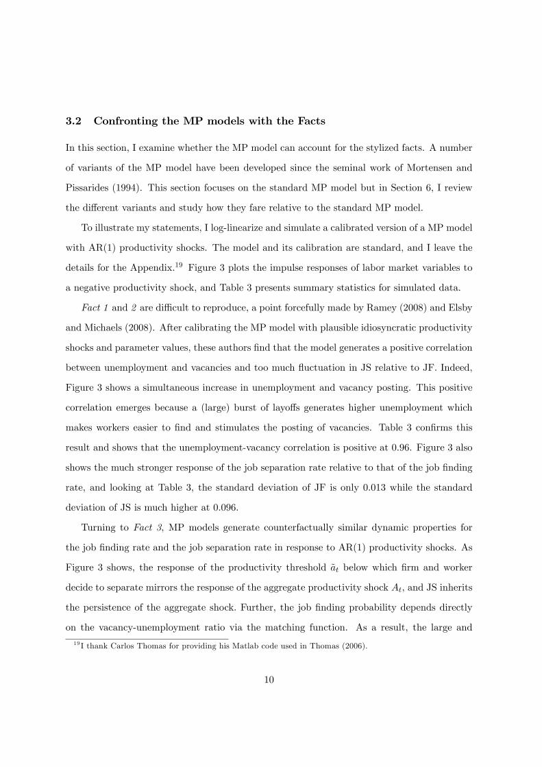
To illustrate my statements, I log-linearize and simulate a calibrated version of a MP model

with AR(1) productivity shocks. The model and its calibration are standard, and I leave the

details for the Appendix.19 Figure 3 plots the impulse responses of labor market variables to

a negative productivity shock, and Table 3 presents summary statistics for simulated data.

Fact 1 and 2 are di¢ cult to reproduce, a point forcefully made by Ramey (2008) and Elsby

and Michaels (2008). After calibrating the MP model with plausible idiosyncratic productivity

shocks and parameter values, these authors �nd that the model generates a positive correlation

between unemployment and vacancies and too much �uctuation in JS relative to JF. Indeed,

Figure 3 shows a simultaneous increase in unemployment and vacancy posting. This positive

correlation emerges because a (large) burst of layo¤s generates higher unemployment which

makes workers easier to �nd and stimulates the posting of vacancies. Table 3 con�rms this

result and shows that the unemployment-vacancy correlation is positive at 0:96. Figure 3 also

shows the much stronger response of the job separation rate relative to that of the job �nding

rate, and looking at Table 3, the standard deviation of JF is only 0:013 while the standard

deviation of JS is much higher at 0:096.

Turning to Fact 3, MP models generate counterfactually similar dynamic properties for

the job �nding rate and the job separation rate in response to AR(1) productivity shocks. As

Figure 3 shows, the response of the productivity threshold ~at below which �rm and worker

decide to separate mirrors the response of the aggregate productivity shock At, and JS inherits

the persistence of the aggregate shock. Further, the job �nding probability depends directly

on the vacancy-unemployment ratio via the matching function. As a result, the large and

19 I thank Carlos Thomas for providing his Matlab code used in Thomas (2006).

10

persistent increase in job separation leads to a persistent decrease in labor market tightness,

and hence to a persistent fall in JF. Thus, JF and JS display very similar impulse responses

and share the same autocorrelation coe¢ cient (Table 3). However, Figure 2 shows that in the

data, the job separation rate returns faster to its long run level than the job �nding rate, and

Table 2 shows that JS is a lot less persistent than JF.

4 A search and matching model with endogenous separation

In this section, I present a search and matching model in which endogenous separation is driven

by demand constraints.

4.1 The model

I develop a partial equilibrium model in which �rms are demand constrained. Since my goal

is to evaluate the model along the labor market dimension, I follow a reduced-form approach

that allows for more tractability and facilitates computation.20

This search model is similar to Krause and Lubik (2007) in that it assumes large demand-

constrained �rms with many workers. However, unlike Krause and Lubik (2007), there are no

match-speci�c productivity shocks, and job separation does not depend on the productivity of

each match. Instead, when faced with lower than expected demand, �rms can choose to layo¤

extra workers to save on labor costs.

Firms and the labor market

I consider an economy populated by a continuum of households of measure one and a continuum

of �rms of measure one. At each point in time, �rm i needs to satisfy demand for its product

20Thanks to the reduced-form approach, the model has only two state variables and is easier to solve nu-merically. In the Appendix, I show that this partial-equilibrium model is a reduced-form version of a generalequilibrium model with monopolistically competitive �rms and nominal rigidities.

11

ydit and hires Nit workers to produce a quantity

ysit = Nith�it (1)

where I normalize the aggregate technology index to one, and hit is the number of hours

supplied by each worker and 0 < � � 1.21

In a search and matching model of the labor market, workers must be hired from the

unemployment pool through a costly and time-consuming job creation process. Firms post

vacancies at a unitary cost c (in units of utility of consumption), and unemployed workers

search for jobs. Vacancies are matched to searching workers at a rate that depends on the

number of searchers on each side of the market. I assume that the matching function takes

the usual Cobb-Douglas form so that the �ow mt of successful matches within period t is

given by mt = m0u�t v1��t where m0 is a positive constant, � 2 (0; 1), ut denotes the number of

unemployed and vt=R 10 vitdi the total number of vacancies posted by all �rms. Accordingly,

the probability of a vacancy being �lled in the next period is q(�t) � m(ut; vt)=vt = m0���

where �t � vtutis the labor market tightness. Similarly, the probability for an unemployed

worker to �nd a job is JFt = (ut; vt)=ut = m0�1��t . Because of hiring frictions, a match formed

at t will only start producing at t+1. Matches are terminated at an exogenous rate �� but the

�rm can also choose to destroy an additional fraction �it of its jobs, so that the job separation

rate JSt = ��+ �it.

The timing of the model is similar to that of Krause and Lubik (2007). Denote n�it the

employment of �rm i at the beginning of period t. Once the uncertainty is resolved, �rms can

decide whether to lay-o¤ a fraction �it of its employment n�it in order to begin production with

n+it = (1��it)n�it workers and pay the corresponding wage bill. At the end of the period, q(�t)vit

matches are created but an additional fraction �� of �rm�s beginning of period employment n�it21The model does not explicitly consider capital for tractability reasons but (1) can be rationalized by assuming

a constant capital-worker ratio KitNit

and a standard Cobb-Douglas production function yit = At (Nithit)�K1��

it .Assuming instead decreasing returns in employment does not change the conclusions of the paper. Similarly,assuming � = 1 does not change any of the results.

12

is destroyed.22 The �rm enters next period with n�it+1 = (1� ��� �it)n�it + q(�t)vit workers.

From now on, I will only consider the beginning of period employment nit = n�it , so that

for a �rm i posting vit vacancies at date t, its the law of motion for employment is given by

nit+1 = (1� ��� �it)nit + q(�t)vit

and its production function takes the form

ysit = (1� �it)nith�it:

Households

I follow Merz (1995) and Andolfatto (1996) in assuming that households form an extended

family that pools its income. There are 1�nt unemployed workers who receive unemployment

bene�ts b in units of utility of consumption, and nt employed workers who receive the wage

payment wit from �rm i for providing hours hit. Consequently, the value of unemployment Ut

in terms of current consumption is

Ut =b

�t+ �Et [JFt+1Wt+1 + (1� JFt+1)Ut+1]

and the value Wit from employment for a worker working for �rm i in terms of current con-

sumption is

Wit = wit ��h

�t (1 + �h)h1+�hit + �Et [(1� JSt+1)Wit+1 + JSt+1Ut+1]

where �h and �h are positive constants and �t = 1Ctthe marginal utility of consumption with

Ct =

�R 10 C

"�1"

it di

� ""�1

; " > 1.

22Labor market tightness is given by �t =R 10 vitdi

1�R 10 (1��it)n

�itdi

.

13

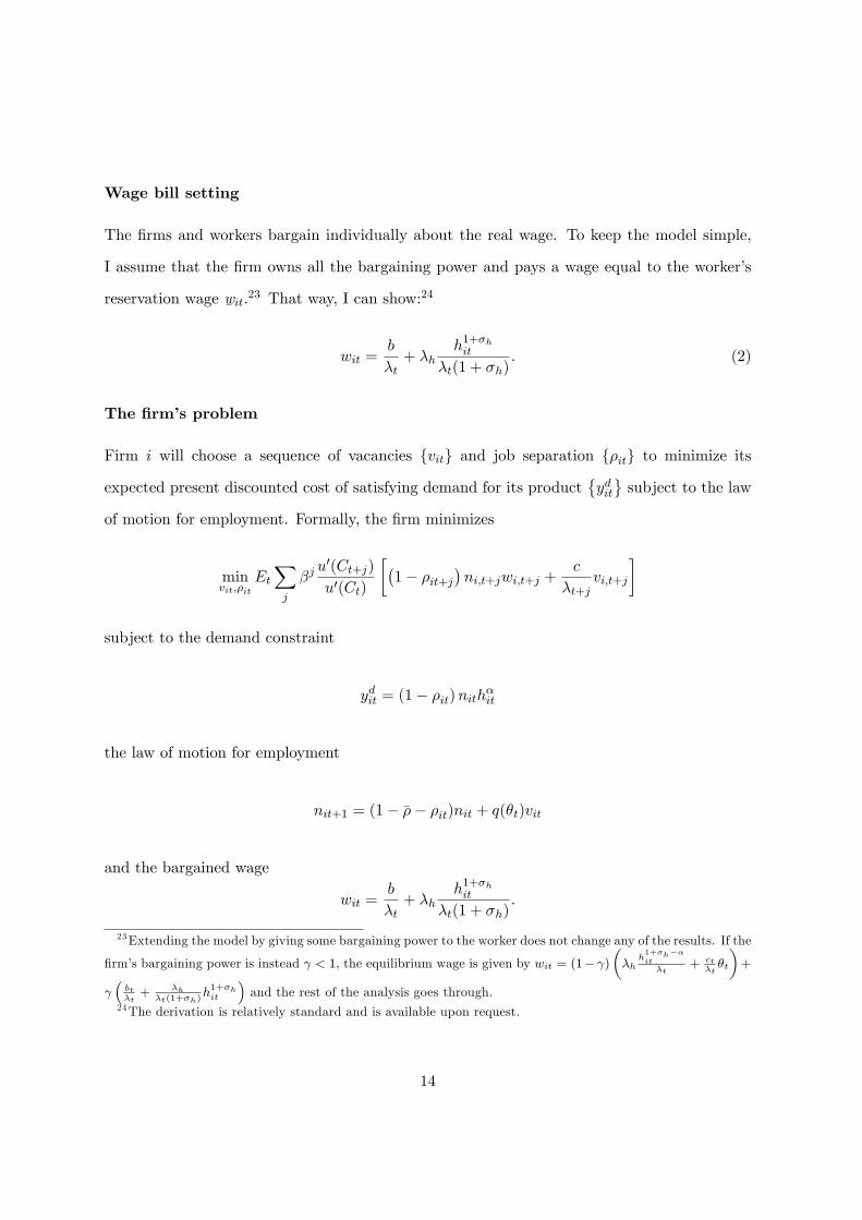
Wage bill setting

The �rms and workers bargain individually about the real wage. To keep the model simple,

I assume that the �rm owns all the bargaining power and pays a wage equal to the worker�s

reservation wage w¯ it.23 That way, I can show:24

wit =b

�t+ �h

h1+�hit

�t(1 + �h): (2)

The �rm�s problem

Firm i will choose a sequence of vacancies fvitg and job separation f�itg to minimize its

expected present discounted cost of satisfying demand for its product�yditsubject to the law

of motion for employment. Formally, the �rm minimizes

minvit;�it

EtXj

�ju0(Ct+j)

u0(Ct)

��1� �it+j

�ni;t+jwi;t+j +

c

�t+jvi;t+j

�

subject to the demand constraint

ydit = (1� �it)nith�it

the law of motion for employment

nit+1 = (1� ��� �it)nit + q(�t)vit

and the bargained wage

wit =b

�t+ �h

h1+�hit

�t(1 + �h):

23Extending the model by giving some bargaining power to the worker does not change any of the results. If the

�rm�s bargaining power is instead < 1, the equilibrium wage is given by wit = (1� )��h

h1+�h��it�t

+ ct�t�t

�+

�bt�t+ �h

�t(1+�h)h1+�hit

�and the rest of the analysis goes through.

24The derivation is relatively standard and is available upon request.

14

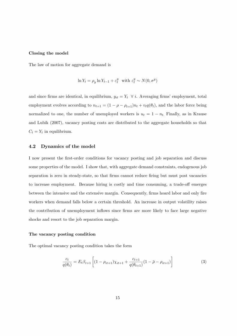
Closing the model

The law of motion for aggregate demand is

lnYt = �y lnYt�1 + "yt with "yt � N(0; �y)

and since �rms are identical, in equilibrium, yit = Yt 8 i. Averaging �rms�employment, total

employment evolves according to nt+1 = (1� �� �t+1)nt + vtq(�t), and the labor force being

normalized to one, the number of unemployed workers is ut = 1 � nt. Finally, as in Krause

and Lubik (2007), vacancy posting costs are distributed to the aggregate households so that

Ct = Yt in equilibrium.

4.2 Dynamics of the model

I now present the �rst-order conditions for vacancy posting and job separation and discuss

some properties of the model. I show that, with aggregate demand constraints, endogenous job

separation is zero in steady-state, so that �rms cannot reduce �ring but must post vacancies

to increase employment. Because hiring is costly and time consuming, a trade-o¤ emerges

between the intensive and the extensive margin. Consequently, �rms hoard labor and only �re

workers when demand falls below a certain threshold. An increase in output volatility raises

the contribution of unemployment in�ows since �rms are more likely to face large negative

shocks and resort to the job separation margin.

The vacancy posting condition

The optimal vacancy posting condition takes the form

ctq(�t)

= Et�t+1

�(1� �it+1)�it+1 +

ct+1q(�t+1)

(1� ��� �it+1)�

(3)

15

with �it, the shadow value of a marginal worker, given by

�it = �@nitwit@nit

= �wit (hit) +1

�hit@wit@hit

Since 1q(�t)

is the expected duration of a vacancy, equation (3) has the usual interpretation:

each �rm posts vacancies until the expected cost of hiring a worker ctq(�t)

equals the expected

discounted future bene�ts��it+j

1j=1

from an extra worker. Because the �rm is demand

constrained, the �ow value of a marginal worker is not his contribution to revenue but his

reduction of the �rm�s wage bill. The �rst term of �it is the wage payment going to an extra

worker, while the second term represents the savings due to the decrease in hours and e¤ort

achieved with that extra worker. Indeed, looking at the wage equation (2), we can see that the

�rm can reduce hours per worker and lower the wage bill by increasing its number of workers.

With �it > 0, the marginal worker reduces the cost of satisfying a given level of demand.

Similarly to Woodford�s (2004) New-Keynesian model with endogenous capital, the marginal

contribution of an additional worker is to reduce the wage bill through substitution of one

input for another. Here, the intensive and the extensive margins are two di¤erent inputs. The

former is �exible but costly, while the latter takes time and resources to adjust. The �rm

chooses the combination of labor margins that minimizes the cost of supplying the required

amount of output.

Using the wage equation (2), I can rewrite the marginal worker�s value as

�it = �b

�t+

�1 + �h�

� 1��h

h1+�hit

�t (1 + �h): (4)

Since hit =�

ydit(1��it)nit

� 1�and nit is a state variable, the �rm relies on the intensive margin to

satisfy demand in the short-run, and the level of hours per worker captures �demand pressures�

and the �rm�s incentives to post vacancies. With 1+�h� > 1, the longer hours are, the larger

is the wage bill reduction obtained with an extra worker. As hours increase because of higher

demand for the �rm�s products, the worker�s marginal value increases, and the �rm posts more

16

vacancies to increase employment. Indeed, 1+�h� � 1 measures the di¤erence between the two

labor inputs (the intensive and the extensive margins) in terms of the cost of providing the

required amount of output. The intensive margin displays decreasing returns with �<1 and

its cost increases at the rate 1+�h so that the cost of producing a given quantity ydit increases

at the rate 1+�h� > 1. For the extensive margin, on the other hand, both output and costs

increase linearly, so that the rate is one. The larger the di¤erence between the two rates, the

stronger is the incentive for the �rm to avoid increases in hours per worker, and the more

volatile are vacancy posting and unemployment.

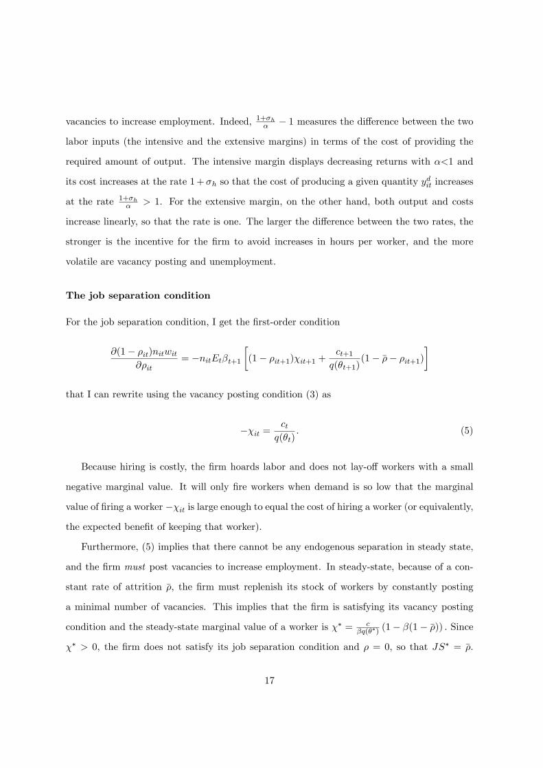
The job separation condition

For the job separation condition, I get the �rst-order condition

@(1� �it)nitwit@�it

= �nitEt�t+1�(1� �it+1)�it+1 +

ct+1q(�t+1)

(1� ��� �it+1)�

that I can rewrite using the vacancy posting condition (3) as

��it =ctq(�t)

: (5)

Because hiring is costly, the �rm hoards labor and does not lay-o¤ workers with a small

negative marginal value. It will only �re workers when demand is so low that the marginal

value of �ring a worker ��it is large enough to equal the cost of hiring a worker (or equivalently,

the expected bene�t of keeping that worker).

Furthermore, (5) implies that there cannot be any endogenous separation in steady state,

and the �rm must post vacancies to increase employment. In steady-state, because of a con-

stant rate of attrition ��, the �rm must replenish its stock of workers by constantly posting

a minimal number of vacancies. This implies that the �rm is satisfying its vacancy posting

condition and the steady-state marginal value of a worker is �� = c�q(��) (1� �(1� ��)) : Since

�� > 0, the �rm does not satisfy its job separation condition and � = 0, so that JS� = ��.

17

Starting from the steady-state equilibrium, a positive shock does not lead to a burst of �un-

�ring�as the �rm cannot lower �it � 0 (i.e. keep workers that it would have otherwise �red)

and must use the job creation margin.

To visualize the mechanisms driving vacancy posting and job separation, Figure 4 plots the

relationship between the marginal value of a worker and hours per worker, a proxy for �demand

pressure�. In steady-state, the value of a marginal worker is positive and equals the net cost

of hiring. When demand goes up, hours per worker increase and with them the marginal value

of a worker, leading the �rm to post more vacancies. For small negative shocks such that

� ctq(�t)

� �it � 0, the �rm hoards labor and posts fewer vacancies. For large negative shocks,

however, �it � � ctq(�t)

, and the �rm uses the job separation margin, and one can observe a

burst of layo¤s.25

Finally, an implication of labor hoarding is that an increase in output volatility raises the

contribution of the job separation rate to unemployment �uctuations since the �rm is more

likely to face large negative shocks and resort to the job separation margin. For the same

reason, the asymmetric behavior of unemployment will be less pronounced in times of lower

output volatility.

5 Confronting the model with the data

In this section, I study whether a calibrated version of the model generates realistic impulse

response functions, can quantitatively account for the stylized facts about unemployment and

its transition probabilities, and can rationalize the small and declining contribution of unem-

ployment in�ows, the increase in gross hiring during recessions as well as the weaker asymmetry

in unemployment since 1985.

25Note that the �rm�s behavior is consistent with the establishment level evidence from Davis, Faberman andHaltiwanger (2006).

18

5.1 Calibration

First, I discuss the calibration of the model; and Table 4 lists the parameter values. An attrac-

tive feature of the model is its small number of (standard) parameters. Whenever possible, I

use the values typically used in the literature. I assume a monthly frequency, as a monthly

calibration is better able to capture the high rate of job �nding in the US. I set the monthly

discount factor � to 0:993 and the returns to hours � to 0:65. Turning to the labor market,

I set the matching function elasticity to � = 0:72 as in Shimer (2005). I set the exogenous

component of the separation rate to 0.032, which is the average value of the 5-year rolling

lower-bound of Shimer�s (2007) employment exit probability series.26 A worker �nds a job

with probability �q(�) = 0:3 so that equilibrium unemployment equals 10 percent.27 The scale

parameter of the matching functionsm0 is chosen such that, as in den Haan and Kaltenbrunner

(2009), a �rm �lls a vacancy with a probability q(�) = 0:34. Shimer (2005) sets the income

replacement ratio to 40 percent, so that with a labor income share of 65 percent, the unemploy-

ment bene�ts-output ratio b = 0:28. The steady-state ratio of vacancy-posting costs to GDP

is set to 1% following most of the literature.28 As in Trigari (2009) and Christo¤el, Kuester

and Linzert (2006), I choose �h = 10, i.e. an hours per worker elasticity of 0:1. Finally, I

set the standard deviation of output �y = 0:0014 and the �rst-order coe¢ cient �y = 0:93 in

order to match the persistence and volatility of HP-detrended real GDP, converted to monthly

frequency. I numerically solve the model using policy function iterations with intergrid cubic

spline interpolation on a grid with (30; 30) points for (nt; yt). Employment nt is discretized

over [0:8; 1], and I follow Tauchen (1986) to construct the transition matrix for yt. In the

Appendix, I describe the numerical algorithm used to solve the �rm�s problem

26Recall that endogenous separation cannot be negative in the model, so that the empirical counterpart ofthe exogenous job separation rate �� is the lower bound of JS. Since JS displays low-frequency movements (seee.g. Davis, 2008) that I abstract from in this paper, I estimate �� as the mean of the 5-year rolling lower-boundof JS. The results of the paper do not rely on this particular estimate of ��.27This value implies a steady-state unemployment equal to 10 percent, which is reasonable if, as in Merz (1995),

Andolfatto (1996), den Haan, Ramey, and Watson (2000) and others, model unemployment also includes thoseindividuals registered as inactive that are actively searching.28See e.g. Andolfatto (1996), Blanchard and Gali (2006) and Gertler and Trigari (2009).

19

5.2 Impulse response functions

Figure 5 and 6 show the simulated impulse response functions of unemployment, hours per

worker, the job �nding rate, and the job separation rate after respectively a positive and a

negative one standard-deviation aggregate demand shock. The asymmetric nature of the labor

market is clearly apparent. Following a positive aggregate demand shock, unemployment

declines progressively while hours per worker react on impact. After two quarters, hours per

worker are back to their long-run value while unemployment starts its mean reversion. After

a negative shock, however, unemployment responds on impact because of a burst of layo¤s.

Thanks to the strong response of the job separation rate, �rms rely less on their intensive

margin and make a smaller adjustment to their number of posted vacancies. Note that vacancy

posting decreases but does not drop to zero, so that the �rms are simultaneously �ring and

posting vacancy.29 This is due to the AR(1) structure of the shocks hitting the economy. Since

hiring takes one period and since shocks are mean-reverting, the �rm anticipates the need for

future higher employment and post vacancies (albeit less so than in normal times) to satisfy

the expected increase in demand next period.30

Because it is costless to adjust the number of workers through the separation margin, layo¤s

show no persistence: �rms �re as many workers as necessary, and endogenous job separation

reverts quickly to zero. The job �nding rate, on the other hand, is persistent and mirrors the

behavior of unemployment after two quarters.

Unlike a standard MP model (see Figure 3) or Krause and Lubik (2007), an increase in job

separation does not lead to an increase in vacancy postings, and unemployment and vacancy

29 Interestingly, this behavior is consistent with establishment level evidence as Davis, Faberman and Halti-wanger (2008) show that �rms with decreasing levels of employment continue to display a positive amount ofvacancy posting and hiring.30 I can prove this result by contradiction. If vacancy posting dropped to zero after a large adverse demand

shock, labor market tightness would drop to zero, and hiring cost would be null. The �rm would then layo¤enough workers to satisfy (5), i.e. �t = 0: In fact, with no hiring frictions, the �rm has no reason to hoardlabor, the problem becomes static and the �rm �res as many workers as necessary to satisfy its current periodoptimal allocation between hours per worker and number of workers. However, with a mean-reverting shockand the additional exogenous job separation occurring between periods, the �rm expects higher demand nextperiod, will need more workers and therefore posts vacancies (at no cost since � = 0). This contradicts myinitial assumption, so that labor market tightness cannot be zero.

20

are negatively correlated. The intuition for these results is as follows. Looking at Figure 4,

�rms use the job separation margin when the marginal value of a worker falls below � ctq(�t)

.

However, after this burst of layo¤s, the marginal value of a worker lies at the boundary between

the labor hoarding region and the lay-o¤ region since �t = � ctq(�t)

. This implies that if aggregate

demand is persistent, the worker�s marginal value in the next period will not be far o¤ the

labor hoarding-layo¤ threshold, and there will not be another large burst of layo¤s. Further,

since the labor hoarding-layo¤ boundary is located in a region in which �rms lower the number

of posted vacancies, the �rm is unlikely to post more vacancies as it lays o¤ workers.31

Finally, Figure 7 shows that the model is consistent with the fact that gross hiring tends

to increase during recessions as well as with Fujita�s (2009) empirical impulse response for

gross hires. A burst of layo¤s decreases labor market tightness and lowers hiring costs as the

expected cost of �lling a vacancy declines. This leads the �rm to pro�t from an exceptionally

low labor market tightness to increase new hires: the job �nding rate goes down but less

than unemployment, and hiring increases. An interesting implication of the model is that this

phenomenon becomes stronger with the size of the shock. As Figure 7 illustrates, the larger

the adverse demand shock, the more the �rm resorts to the job separation margin, the more

labor market tightness decreases and the stronger is the �rm�s incentive to pro�t from lower

hiring costs by increasing gross hires.

5.3 Simulation

Using a calibrated version of the model, I simulate 600 months (i.e. 50 years) of data, and

I repeat this exercise 500 times. I �rst evaluate the model by considering the moments of

simulated data to test whether the model is consistent with the three facts about unemployment

and its transition probabilities. Then I study whether the model can account for the small

and declining contribution of unemployment in�ows, as well as the fact that unemployment

displays no steepness asymmetry since 1985.

31However, this is not necessarily the case if the shock is not persistent. In that case, f�itg is more likely toshift quickly from negative values (with �ring) to positive values (with more vacancies).

21

Table 5 presents the summary statistics for quarterly averages of the monthly series. A

general conclusion is that given the model simplicity and its small number of parameters,

the model is remarkably successful at explaining the behavior of labor market variables: the

moments all have the correct sign and are close to their empirical values.32 First, the model

has no problem generating Fact 1, i.e. a Beveridge curve and a negative job �nding rate-job

separation rate correlation. The model can also explain the strong unemployment-vacancies

correlation (�0:81 versus �0:90 in the data) as well as the weaker JF-JS correlation (�0:59

versus �0:48 in the data). Similarly, and consistent with the data, the model generates a high

job �nding rate-unemployment correlation (�0:91 versus �0:95 in the data) and a smaller job

separation rate-unemployment correlation (0:47 versus 0:61 in the data). These results stem

from the asymmetric nature of the labor market and the fact that �rms can adjust employment

with the job creation margin at all times but can only use the job separation margin for negative

demand shocks. For positive demand shocks, the job separation rate does not move and the

correlation with unemployment or the job �nding rate is nil. As a result, the JS-unemployment

correlation and the JF-JS correlation are closer to a half than to one.

Table 5 also shows that the model is consistent with Fact 2, as the job �nding rate is more

volatile than the job separation rate. The fact that the model has no problem matching the

volatility of the job �nding rate is a result of the demand constraints faced by �rms. In order

to satisfy an expanding demand, �rms must increase either their extensive or their intensive

margin. Since the intensive margin is relatively costly because of the high disutility cost of

longer hours, most of the adjustment occurs through employment.33 Thus, the model does not

su¤er from a Shimer (2005) type puzzle as it generates enough �uctuations in unemployment

given plausible movements in output. Nonetheless, JF is slightly too volatile, a problem with

32 It is important to note that I am only focusing on labor market variables. As long as aggregate demandconstraints persist long enough so that my model is a correct description of �rms�labor demand in the short-run,I can judge of the model�s success by considering the unconditional moments of labor market variables.33From the log-linearized production function y = �h� 1�u

uu , unemployment will be roughly 10 times more

volatile than output (with an unemployment rate around 10 percent) if h is small. Note also that this mechanismis consistent with the data as the volatility in hours per worker generated by the model matches that found inthe data.

22

search models of unemployment already pointed out by Fujita and Ramey (2004). This is

due to the excessively rapid response of vacancies; and incorporating sunk costs for vacancy

creation as in Fujita and Ramey (2004) would presumably correct this shortcoming. Finally,

the job separation rate�s volatility is close to its empirical value. Unlike standard MP models,

the separation margin is only used for large negative shocks as �rms hoard labor and only use

the job separation margin for large negative shocks.

Turning to Fact 3 and the dynamic properties of JF and JS, Figure 8 shows that the model

is very successful at reproducing the cross-correlograms of JF, JS and unemployment. JS is

not persistent enough as most of the adjustment along the job separation margin takes place in

one period, but assuming convex costs in �ring would probably correct this shortcoming. JF

is slightly less persistent than in the data, and this is again due to excessively rapid response

of vacancies. Finally, the low persistence of model JF and JS explains the low persistence of

model hours per worker as the intensive margin adjusts to movements in employment to ensure

that the �rm satis�es demand at all times.

Finally, in Table 6, I follow Shimer (2007), Elsby, Michaels and Solon (2008) and Fujita

and Ramey (2008) and measure the contribution of JF and JS. I �nd that the contribution of

JS amounts to 22%, only slightly lower than the contribution measured by Shimer (2007).

5.4 The weaker contribution of JS since 1985

We saw in Section 2 that the contribution of JS to the variance of unemployment declined from

about 25 percent during the post-war period to only 5 percent over the last 20 years (Shimer,

2007). Moreover, the steepness asymmetry in unemployment disappeared after 1985.

The model implies that these two �ndings are by-products of the Great Moderation, the

period of low macroeconomic volatility enjoyed by the US (and other developed countries)

over 1985-2007. One insight from section 4 was that a decrease in output volatility lowers

the contribution of JS and the asymmetry in unemployment as �rms are less likely to face

large negative shocks and resort to the job separation margin. Figure 6 shows this e¤ect

23

quantitatively. As the size of the shock doubles from one half to one standard-deviation of

detrended GDP, the response of JS on impact more than doubles, and unemployment shows a

stronger initial response. The hours per worker response, on the other hand, does not increase

with the size of the shock.

To evaluate whether the decline in macroeconomic volatility can explain the weaker con-

tribution of JS, I estimate the contribution of JS and JF on simulated data with an output

volatility of �y

2 , consistent with the drop in volatility experienced by the US during the Great

Moderation. As Table 6 shows, the contribution of JS decreases to 14%, suggesting that the

Great Moderation is responsible for some of the decline in the contribution of JS.34

Finally, looking at Table 6, the skewness of model unemployment also declines sharply

when the volatility of output decreases, suggesting that the Great Moderation is responsible

for some of the decline in the asymmetry of unemployment. With an output volatility of �y, the

skewness of model unemployment is 0:53, close to its empirical counterpart of 0:62. But with

a standard-deviation of output is �y

2 , model unemployment shows no evidence of asymmetry,

just as in the data.

6 Related literature

In Section 2, I mainly focused on the canonical Mortensen-Pissarides (1994) search and match-

ing model. However, a number of variants of the MP framework have been used to model

unemployment. In this section, I review the literature on the di¤erent variants and their

empirical performances.

First, while the original MP model assumes persistent idiosyncratic productivity shocks,

the computational cost associated with keeping track of the jobs�productivity distribution lead

many researchers to assume instead i.i.d. idiosyncratic productivity shocks. Indeed, only a

34 I do not claim that this is the only explanation. The increased availability of �exible labor service such aspart-time work and temporary work or the switch from manufacturing to services are probably also responsiblefor the decline in the contribution of the job separation rate. See, for example, Schreft, Sing and Hodgson(2005).

24

few papers solved the original MP model with endogenous separation (Mortensen-Pissarides

(1994), Ramey (2008), Elsby and Michaels (2008), Pissarides (2008)), but a vast literature

has solved rich general equilibrium models with search unemployment and i.i.d. idiosyncratic

productivity shocks: Den Haan, Ramey and Watson (2000), Costain and Reiter (2005), Walsh

(2005), Thomas (2006), Krause and Lubik (2007), Cooper, Haltiwanger and Willis (2008),

Thomas and Zanetti (2008), Trigari (2009) among others.

Second, variants of the MP model can be classi�ed in two categories, depending on whether

�rms are atomistic with only one worker or large with many workers. In their seminal paper,

Mortensen and Pissarides (1994) assume the existence of a �nite mass of workers and of an

in�nite mass of atomistic �rms. Each non-matched �rm can post a vacancy to form a match

with one worker only. Another line of research departs from the assumption of free entry and

atomistic �rms to model instead a �nite number of large �rms with a continuum of jobs.35

This approach has the advantage of allowing for a more realistic representation of the �rm as

well as providing a framework to study the interaction of labor market frictions with other

frictions such as nominal rigidities. While the majority of papers pursued the �rst approach,

Krause and Lubik (2007) provide a tractable example of the second approach in which the

�rms� production function displays constant returns to employment. While aggregation is

more di¢ cult with decreasing returns to employment, Elsby and Michaels (2008) present an

analytically tractable model while Cooper, Haltiwanger and Willis (2008) solve and estimate

a similar model with numerical methods.

Krause and Lubik (2007), for MP models with large �rms, and Costain and Reiter (2005),

Thomas (2006), Ramey (2008) and Elsby and Michaels (2008), for MP models with atomistic

�rms, make the case that Fact 1 is di¢ cult to reproduce. Standard MP models are unable

to replicate the Beveridge curve because a burst of layo¤s generates higher unemployment

which makes workers easier to �nd, stimulating the posting of vacancies. Krause and Lubik

(2007) show that introducing real wage rigidity allows the model to generate a Beveridge

35 In this setup, entry of new �rms is forbidden as otherwise, the model would collapse to the original MPmodel with atomistic �rms and one �rm-one worker matches.

25

curve. However, the model cannot reproduce Fact 2 as ��rms adjust almost exclusively via

the separation rate and job creation does not play a quantitatively signi�cant role� (Krause

and Lubik, 2007, p724). Ramey (2008) shows that a search model with on the job search can

generate a Beveridge curve. However, that model cannot reproduce Fact 2 as it generates

too much volatility in the job destruction rate compared to the job �nding rate (Ramey,

2007, Figure 1). Thomas (2006) shows how �ring costs help the MP model in generating a

Beveridge curve. However, his model cannot generate Fact 3 as the impulse response of JF

counterfactually mirrors that of JS.

While fewer papers other than Ramey (2008) and Elsby and Michaels (2008) focused on

Fact 2, Krause and Lubik (2007) show that in MP models with large �rms, the job separation

rate moves too much compared to the job �nding rate. This is not the case in MP models with

instantaneous hiring and �ring costs (Thomas and Zanetti, 2008) and in MP models with an

intensive labor margin (Trigari, 2009). However, both of these models cannot generate Fact

3 : the impulse response of JF counterfactually mirrors that of JS, displays no persistence and

overshoots its long-run value.

Finally, a very promising line of research is the work from Cooper, Haltiwanger and Willis

(2008) and Elsby and Michaels (2008). By considering large �rms with decreasing returns

to employment and idiosyncratic productivity shocks, they show that such generalized MP

models can generate a Beveridge curve. Elsby and Michaels (2008) show that their model can

generate elasticities of JS and JF with respect to productivity that are consistent with the data.

However, it is di¢ cult to confront these models with the last two stylized Facts as Cooper et

al (2008) do not focus on unemployment �ows and Elsby and Michaels�(2008) model has only

two aggregate productivity states.

7 Conclusion

This paper presents a search model with a demand-driven job separation mechanism that can

account for both the out�ows and the in�ows of unemployment. Despite a relatively small num-

26

ber of parameters, the model is successful at explaining the behavior of labor market variables

and is consistent with a low, but non-trivial, contribution of JS to unemployment �uctuations.

On the other hand, the benchmark framework, the Mortensen-Pissarides search and matching

model with endogenous separation, has di¢ culties explaining the low contribution of JS as

well as other stylized facts.

In addition, my model attributes the decrease in the contribution of JS since 1985 to the

Great Moderation, the dramatic drop in macroeconomic volatility enjoyed by the US economy

from the mid 80s until 2007. It also implies that the lower contribution of JS was a temporary

phenomenon and that the importance of JS would increase in times of higher macroeconomic

volatility such as the in current (since December 2007) recession.36

While a demand-driven job separation mechanism shows promises towards an equilibrium

model of unemployment with endogenous out�ows and in�ows, an important extension of

this model would be to incorporate idiosyncratic (productivity or demand) shocks to allow

for �rm heterogeneity. Moreover, embedding the model in a general equilibrium framework

would allow me to study the implications of labor market asymmetries on output and in�ation.

Because increasing employment is more costly than lowering employment, �rms tend to adjust

prices rather than quantities after positive monetary shocks but do the opposite after monetary

contractions. As a result, monetary policy would have a stronger ability to lower, than to raise,

output. I leave these topics for future research.

36 In Barnichon (2009), I provide some evidence supporting this possibility.

27

Appendix:

A.1 A Mortensen-Pissarides (1994) model with i.i.d. idiosyncratic produc-

tivity shocks

I follow Thomas (2006), and I present an MP model with a �nite mass of workers and an

in�nite mass of atomistic �rms. Each non-matched �rm can post a vacancy to form a match

with one worker only. Workers are hired from the unemployment pool through a costly and

time-consuming job creation process. Firms post vacancies at a unitary cost c, and unemployed

workers search for jobs. Vacancies are matched to searching workers at a rate that depends

on the number of searchers on each side of the market. The matching function takes the

usual Cobb-Douglas form so that the �ow mt of successful matches within period t is given by

mt = m0u�t v1��t : Accordingly, the probability of a vacancy being �lled in the next period is

q(�t) � m(ut; vt)=vt = m0��� where �t � vt

ut, and the probability for an unemployed worker to

�nd a job is p(�t) = (ut; vt)=ut = m0�1��t .

In this economy, jobs are subject to idiosyncratic productivity shocks drawn from a distri-

bution with the log-normal cdf F (a), and there exists a threshold productivity ~at such that

all jobs with productivity below it yield a negative surplus are destroyed. Therefore, total

separation rate is JSt = ��+ (1� ��)F (~at) with �� the exogenous separation rate, and the law of

motion for employment is nt = (1� JSt)nt�1 +m(ut�1; vt�1).

New jobs have maximum productivity aN . The value of continuing a match with idiosyn-

cratic productivity at and aggregate productivity At is given by

Jt(at) = Atat � wt(at) + Et�(1� ��)1Z

~at+1

Jt+1(a)dF (a):

The assumption of free entry and exits of �rms ensures that the value of posting a vacancy is

zero so that

Vt = 0 = �c+ q(�t)Et�Jt+1(aN ):

28

The value that a worker enjoys from holding a job with productivity at is given by

Wt(at) = wt(at) + Et�

264(1� ��) 1Z~at+1

Jt+1(a)dF (a) + �t+1Ut+1

375and the value of being unemployed is

Ut = b+ Et��p(�t)W

Nt+1 + (1� p(�t))Ut+1

�:

In each period, �rm and worker Nash bargain over the real wage and we have wt(at) = Atat+

c�t + (1� )b:

The familiar job destruction condition is then given by Jt(~at) = 0 or

At~at � b�

1� c�t + Et�(1� �)1Z

~at+1

At+1(a� ~at+1)dF (a) = 0

and the job creation condition takes the form

c

q(�t)= (1� )Et�

�At+1(a

N � ~at+1)�:

I then solve the model by log-linearizing around the steady-state. For the calibration, I

use the same parameter values as in this paper�s model (see Table 4) whenever possible. For

other parameters, I follow Thomas (2006). The aggregate productivity shock At follows an

AR(1) process such that lnAt = �A lnAt�1 + "t with �A = 0:95 and the standard-deviation

�A calibrated to match the cyclical volatility of detrended US real output. Idiosyncratic

productivity ln at has mean �a = 0 and standard-deviation �a = 0:22 as in Ramey (2008) and

Elsby and Michaels (2008).

29

A.2 A New-Keynesian search model with endogenous separation

Households

I consider an economy populated by a continuum of households of measure one and a continuum

of �rms of measure one. With equilibrium unemployment, ex-ante homogenous workers become

heterogeneous in the absence of perfect income insurance because each individual�s wealth

di¤ers based on his employment history. To avoid distributional issues, I follow Merz (1995) and

Andolfatto (1996) in assuming that households form an extended family that pools its income

and chooses per capita consumption and assets holding to maximize its expected lifetime utility.

There are 1� nit unemployed workers who receive unemployment bene�ts b in units of utility

of consumption, and nit employed workers who receive the wage payment wit from �rm i for

providing hours hit. Denoting g(hit) the individual disutility from working, the representative

family seeks to maximize

E0

1Xt=0

�t�ln (Ct) + �m ln(

Mt

Pt)� �h

1 + �h

Z 1

0nith

1+�hit di

�

subject to the budget constraint

Z 1

0PjtCjtdj +Mt =

Z 1

0nitwitdi+ (1� nt)bCt +�t +Mt�1

with �m, �h, �h > 0, nt =R 10 nitdi, Mt nominal money holdings, �t total transfers to the

family and Ct the composite consumption good index de�ned by Ct =�R 1

0 C"�1"

it di

� ""�1where

Cit is the quantity of good i 2 [0; 1] consumed in period t and Pit is the price of variety i: " > 1

is the elasticity of substitution among consumption goods. The aggregate price level is de�ned

as Pt =

0@ 1Z0

P 1�"it di

1A1

1�"

.

30

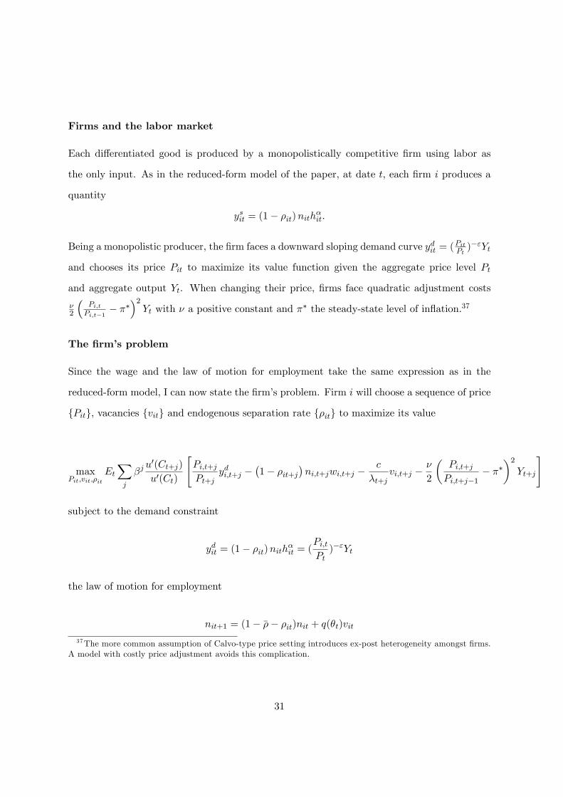
Firms and the labor market

Each di¤erentiated good is produced by a monopolistically competitive �rm using labor as

the only input. As in the reduced-form model of the paper, at date t, each �rm i produces a

quantity

ysit = (1� �it)nith�it:

Being a monopolistic producer, the �rm faces a downward sloping demand curve ydit = (PitPt)�"Yt

and chooses its price Pit to maximize its value function given the aggregate price level Pt

and aggregate output Yt. When changing their price, �rms face quadratic adjustment costs

�2

�Pi;tPi;t�1

� ���2Yt with � a positive constant and �� the steady-state level of in�ation.37

The �rm�s problem

Since the wage and the law of motion for employment take the same expression as in the

reduced-form model, I can now state the �rm�s problem. Firm i will choose a sequence of price

fPitg, vacancies fvitg and endogenous separation rate f�itg to maximize its value

maxPit;vit;�it

EtXj

�ju0(Ct+j)

u0(Ct)

"Pi;t+jPt+j

ydi;t+j ��1� �it+j

�ni;t+jwi;t+j �

c

�t+jvi;t+j �

�

2

�Pi;t+jPi;t+j�1

� ���2Yt+j

#

subject to the demand constraint

ydit = (1� �it)nith�it = (Pi;tPt)�"Yt

the law of motion for employment

nit+1 = (1� ��� �it)nit + q(�t)vit37The more common assumption of Calvo-type price setting introduces ex-post heterogeneity amongst �rms.

A model with costly price adjustment avoids this complication.

31

and the bargained wage

wit =b

�t+ �h

h1+�hit

�t(1 + �h):

The central bank

The money supply evolves according to Mt = ea:t+mt with mt = �mmt�1+ "mt , �m 2 [0; 1] and

"mt � N(0; �m): I interpret "mt as an aggregate demand shock.

Closing the model

Averaging �rms�employment, total employment evolves according to nt+1 = (1� ��� �t)nt +

vtq(�t): The labor force being normalized to one, the number of unemployed workers is ut =

1 � nt. Finally, as in Krause and Lubik (2007), vacancy posting costs are distributed to the

aggregate households so that Ct = Yt in equilibrium.

The price setting condition

The vacancy posting condition and the job separation condition are identical to the ones I

report in the paper, and I do not repeat them here. For the price-setting condition, I get the

standard result for models with quadratic price adjustment

(1� ")yitPt� " yit

Pitsit � �

ytPit�1

�PitPit�1

� ���= Et�t+1�yt+1 (�t+1 � ��)

Pit+1P 2it

with the real marginal cost sit given by

sit =@(1� �it)witnit

@yit

=1

��hh

1+�h��it Yt

In order to produce an extra unit of output, the �rm needs to increase hours since employment

is a state variable. As a result, the wage response to changes in hours is driving the �rm�s

32

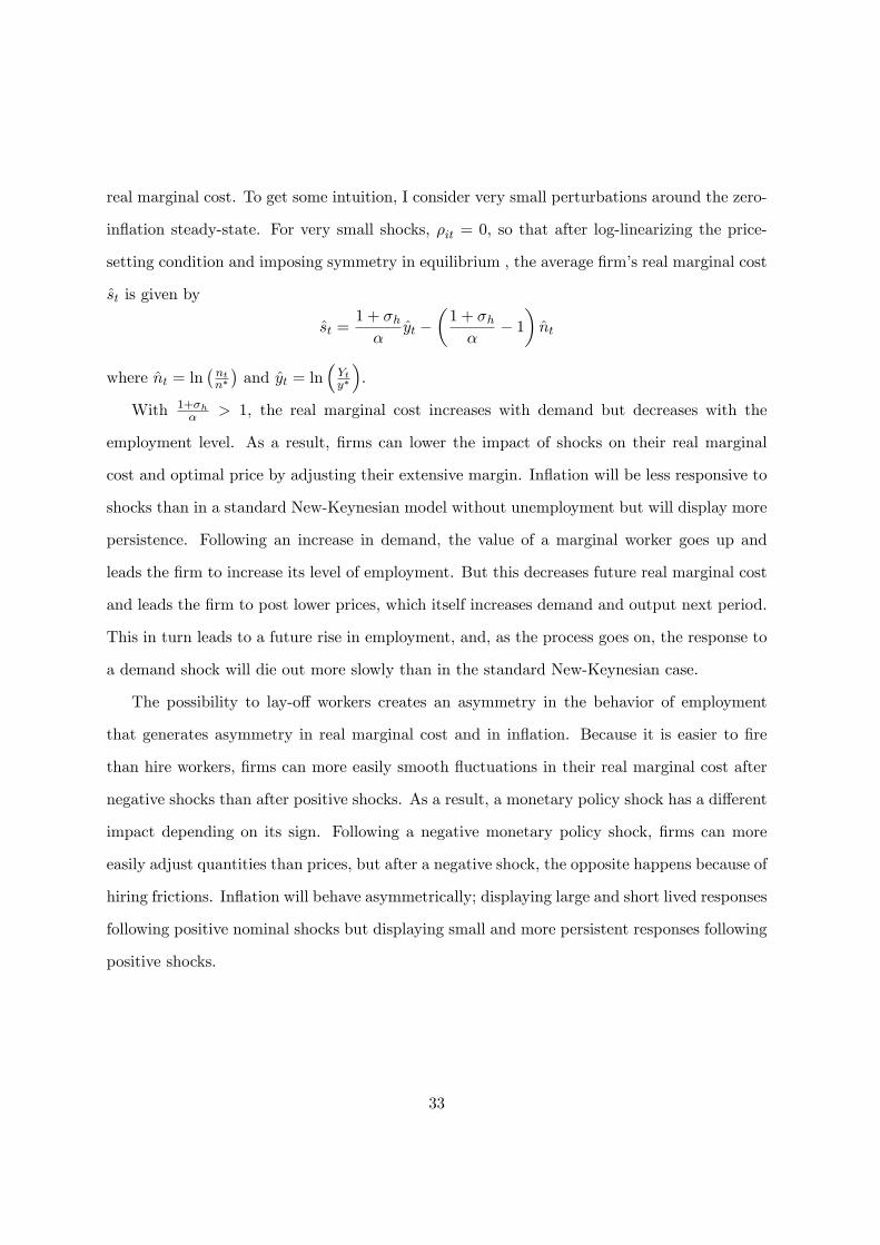
real marginal cost. To get some intuition, I consider very small perturbations around the zero-

in�ation steady-state. For very small shocks, �it = 0, so that after log-linearizing the price-

setting condition and imposing symmetry in equilibrium , the average �rm�s real marginal cost

st is given by

st =1 + �h�

yt ��1 + �h�

� 1�nt

where nt = ln�ntn��and yt = ln

�Yty�

�.

With 1+�h� > 1, the real marginal cost increases with demand but decreases with the

employment level. As a result, �rms can lower the impact of shocks on their real marginal

cost and optimal price by adjusting their extensive margin. In�ation will be less responsive to

shocks than in a standard New-Keynesian model without unemployment but will display more

persistence. Following an increase in demand, the value of a marginal worker goes up and

leads the �rm to increase its level of employment. But this decreases future real marginal cost

and leads the �rm to post lower prices, which itself increases demand and output next period.

This in turn leads to a future rise in employment, and, as the process goes on, the response to

a demand shock will die out more slowly than in the standard New-Keynesian case.

The possibility to lay-o¤ workers creates an asymmetry in the behavior of employment

that generates asymmetry in real marginal cost and in in�ation. Because it is easier to �re

than hire workers, �rms can more easily smooth �uctuations in their real marginal cost after

negative shocks than after positive shocks. As a result, a monetary policy shock has a di¤erent

impact depending on its sign. Following a negative monetary policy shock, �rms can more

easily adjust quantities than prices, but after a negative shock, the opposite happens because of

hiring frictions. In�ation will behave asymmetrically; displaying large and short lived responses

following positive nominal shocks but displaying small and more persistent responses following

positive shocks.

33

A.3 Computation

I solve the model with policy function iteration by simultaneously solving the two �rst-order

conditions for vacancy posting and job destruction:

ctq(�t)

= Et�t+1

�(1� �t+1)�t+1 +

ct+1q(�t+1)

(1� ��� �t+1)�

(6)

��t =ctq(�t)

if �t < 0 (7)

with �t = � b�t+�1+�h� � 1

��h

h1+�ht

�t(1+�h)the value of a marginal worker.

I use policy function iterations with intergrid cubic spline interpolation on a grid with

(30; 30) points for the two state variables nt and yt. Employment nt is discretized over [0:8; 1],

and I follow Tauchen�s method (1986) to represent the AR(1) process yt as a Markov chain.

Since employment will only rarely take extreme values, I allow for a higher grid density for

employment around its steady-state value.

The general algorithm is as follows:

1. Guess policy functions for �0(ni; yj) and �0(ni; yj) and interpolate their values with

intergrid cubic spline interpolation for points not on the grid

2. For all ni and yj :

a. If ��(�0(ni; yj); �0(ni; yj)) > ctq(�0(ni;yj))

�1(ni; yj) = 0 and �nd �1(ni; yj) to satisfy (6) using interpolated �0 and �0 to compute

the right-hand side of (6).

b. Otherwise, solve jointly (6) and (7) for �1(ni; yj) and �1(ni; yj):

3. Repeat 2. until k �1 � �0 k< "� and k �1 � �0 k< "�:

Since it is computationally demanding to jointly solve for � and �, I restrict this joint

calculation to the �rst and latter steps of the computation loop. More precisely, I start with a

loose value for "� so that once I obtain a decent approximation for �, I only iterate on � taking

the policy rule � as given. When � converges to a good approximation, I resume solving for

34

both � and � simultaneously.

35

References

[1] Andolfatto, D. �Business Cycles and Labor-Market Search,�American Economic Review,

86(1), 1996.

[2] Barnichon, R. �Productivity, Aggregate Demand and Unemployment Fluctuations,�Fi-

nance and Economics Discussion Series 2008-47, Board of Governor of the Federal Reserve

System, 2008.

[3] Barnichon, R. �Vacancy Posting, Job Separation, and Unemployment Fluctuations,�

Mimeo, 2009.

[4] Blanchard, O. and P. Diamond, �The cyclical behavior of the gross �ows of U.S. workers,�

Brookings Papers on Economic Activity, 2, pp. 85�155, 1990.

[5] Canova, F., C. Michelacci and D. López-Salido, �Schumpeterian Technology Shocks,�

mimeo CEMFI, 2007.

[6] Christo¤el, K., K. Kuester and T. Linzert, �Identifying the Role of Labor Markets for

Monetary Policy in an Estimated DSGE Model,�ECB Working Paper No 635, 2006.

[7] Cooper, R., J. Haltiwanger and J. Willis, �Search frictions: Matching aggregate and

establishment observations,�Journal of Monetary Economics, 54 pp. 56-78, 2008.

[8] Costain, J. S. and M. Reiter �Business cycles, unemployment insurance, and the cal-

ibration of matching models,� Journal of Economic Dynamics and Control, 32(4), pp

1120-1155, 2007.

[9] Davis, S. �The Decline of Job Loss and Why It Matters,�American Economic Review

P&P, 98(2), pp. 263-267, 2008.

[10] Davis, S. and J. Haltiwanger. �The Flow Approach to Labor Markets: New Data Sources

and Micro-Macro Links,�Journal of Economic Literature, 20(3), pp. 3-26, 2006.

36

[11] Davis, S., J. Faberman, J. Haltiwanger, R. Jarmin and J. Miranda. �Business Volatility,

Job Destruction and Unemployment,�NBER Working Paper No. 14300, 2008.

[12] den Haan, W. and G. Kaltenbrunner �Anticipated Growth and Business Cycles in Match-

ing Models,�Journal of Monetary Economics, Forthcoming, 2009.

[13] den Haan, W., G. Ramey and J. Watson. �Job Destruction and Propagation of Shocks,�

American Economic Review, 90 (3), pp. 482�498., 2000.

[14] DeLong, B. and L. Summers. �Are Business Cycles Asymmetrical?,�American Business

Cycle: Continuity and Change, edited by R. Gordon. Chicago: University of Chicago

Press, pp 166-79, 1986.

[15] Elsby, M. and R. Michaels �Marginal Jobs, Heterogeneous Firms and Unemployment

Flows,�NBER Working Paper No. 13777, 2008.

[16] Elsby, M. R. Michaels and G. Solon. �The Ins and Outs of Cyclical Unemployment,�

American Economic Journal: Macroeconomics, 2009.

[17] Fujita, S. �Dynamics of Worker Flows and Vacancies: Evidence from the Sign Restriction

Approach,�Journal of Applied Econometrics, Forthcoming, 2009.

[18] Fujita, S. and G. Ramey. �The Cyclicality of Job Loss and Hiring,�Federal Reserve Bank

of Philadelphia, 2006.

[19] Fujita, S. and G. Ramey. �Job Matching and Propagation,�Journal of Economic Dynam-

ics and Control, pp. 3671-3698, 2007.

[20] Fujita, S. and G. Ramey. �The Cyclicality of Separation and Job Finding Rates,�Working

Paper, 2007

[21] Fernald, J. �Trend Breaks, long run Restrictions, and the Contractionary E¤ects of Tech-

nology Shocks,�Working Paper, 2005.

37

[22] Galí, J. �Technology, Employment and The Business Cycle: Do Technology Shocks Ex-

plain Aggregate Fluctuations?,�American Economic Review, 89(1), 1999.

[23] Gertler, M. and A. Trigari �Unemployment Fluctuations with Staggered Nash Wage Bar-

gaining,�Journal of Political Economy, 117(1), 2009.

[24] Hall, R. �Employment E¢ ciency and Sticky Wages: Evidence from Flows in the Labor

Market,�The Review of Economics and Statistics, 87(3), pp. 397-407, 2005.

[25] Hall, R. �Employment Fluctuations with Equilibrium Wage Stickiness,�American Eco-

nomic Review, 95(1), pp. 50-65, 2005.

[26] Hall, R. �Job Loss, Job Finding, and Unemployment in the U.S. Economy over the Past

Fifty Years,�NBER Macroeconomics Annual, pp. 101-137, 2005.

[27] Krause, M and T. Lubik. �The (Ir)relevance of Real Wage Rigidity in the New Keynesian

Model with Search Frictions�, Journal of Monetary Economics, 54 pp. 706-727, 2007.

[28] Mc Kay, A. and R. Reis. �The Brevity and Violence of Contractions and Expansions,�

Journal of Monetary Economics, 55, pp. 738-751, 2008.

[29] Mertz, M. �Search in the Labor Market and the Real Business Cycle,�Journal of Monetary

Economics, 49, 1995.

[30] Michelacci, C. and D. López-Salido. �Technology Shocks and Job Flows,�Review of Eco-

nomic Studies, 74, 2007.

[31] Mortensen, D. and E. Nagypal. �More on Unemployment and Vacancy Fluctuations,�

Review of Economic Dynamics, 10, pp. 327-347, 2007.

[32] Mortensen, D. and C. Pissarides. �Job Creation and Job Destruction in the Theory of

Unemployment,�Review of Economic Studies, 61, pp. 397-415, 1994.

38

[33] Neftci, S. �Are Economic Time Series Asymmetric over the Business Cycle?,�Journal of

Political Economy, 92, pp 307-28, 1984.

[34] Petrongolo, B. and C. Pissarides. �The Ins and Outs of European Unemployment,�Amer-

ican Economic Review P&P, 98(2), 256-262, 2008.

[35] Pissarides, C. Equilibrium Unemployment Theory, 2nd ed, MIT Press, 2000.

[36] Pissarides, C. �The Unemployment Volatility Puzzle: Is Wage Stickiness the Answer?,�

Econometrica, Forthcoming, 2009.

[37] Ramey, G. �Exogenous vs. Endogenous Separation,�Working Paper, 2007.

[38] Schreft, S. A. Singh and A. Hodgson. �Jobless Recoveries and the Wait-and-See Hypoth-

esis,� Economic Journal-Federal Reserve Bank of Kansas City, 4th Quarter, pp 81-99,

2005.

[39] Shimer, R. �The Cyclical Behavior of Equilibrium Unemployment and Vacancies,�Amer-

ican Economic Review, 95(1), pp. 25-49, 2005.

[40] Shimer, R. �Reassessing the Ins and Outs of Unemployment,�NBER Working Paper No.

13421, 2007.

[41] Sichel, D. �Business Cycle Asymmetry: a Deeper Look,�Economic Inquiry, 31, pp. 224-

36, 1993.

[42] Thomas, C. �Firing costs, labor market search and the business cycle",�Working Paper,

2006.

[43] Thomas, C. �Search and matching frictions and optimal monetary policy,� Journal of

Monetary Economics, 55(5), 2008.

[44] Thomas, C. and F. Zanetti. �Labor market reform and price stability: an application to

the Euro Area,�Working Paper, 2008.

39

[45] Trigari, A. �The Role of Search Frictions and Bargaining for In�ation Dynamics,�IGIER

Working Paper, 2006.

[46] Trigari, A. �Equilibrium Unemployment, Job Flows and In�ation Dynamics,�Journal of

Money, Credit and Banking, 2009.

[47] Walsh, C. �Labor Market Search and Monetary Shocks,�in Elements of Dynamic Macro-

economic Analysis, S. Altug, J. Chadha, and C. Nolan, Cambridge University Press, 2004,

451-486.

[48] Woodford, M. �In�ation and Output Dynamics with Firm-Speci�c Investment,�Working

Paper, 2004.

40

Table 1: Skewness, Monthly data

du dy

1951­2007 0.65**(0.19)

0.26(0.36)

1985­2007 0.09(0.08)

0.17(0.12)

Notes: Monthly unemployment u is constructed by the BLS from the CPS, and y is logged realGDP. Both series are seasonally adjusted and detrended with an HP­filter (λ=10,000). Newey­West standard errors are reported in parentheses. ** indicates significance at the 5% level.

Table 2: US Data, 1951­2006

u v µ jf js h yStandarddeviation 0.187 0.198 0.378 0.116 0.065 0.007 0.021

Quarterlyautocorrelation 0.938 0.948 0.946 0.912 0.648 0.83 0.84

u 1 ­0.90 ­0.97 ­0.95 0.61 ­0.50 ­0.69v ­ 1 0.98 0.92 ­0.55 0.63 0.78µ ­ ­ 1 0.96 ­0.62 0.60 0.76jf ­ ­ ­ 1 ­0.48 0.51 0.69js ­ ­ ­ ­ 1 ­0.55 ­0.56h ­ ­ ­ ­ ­ 1 0.81

Correlationmatrix

y ­ ­ ­ ­ ­ ­ 1Notes: Seasonally adjusted unemployment u is constructed by the BLS from the Current Population Survey (CPS). The seasonally adjusted help­wanted advertising index v is constructedby the Conference Board. Labor market tightness is the vacancy­unemployment ratio. jf and js are the quarterly job finding probability and employment exit probability series constructedby shimer (2007). Hours per worker h only covers 1956­2006 and is the sum of the quarterly average of weekly manufacturing overtime of production workers and the average over 1956­2006 of weekly regular manufacturing hours of production workers from the Current Employment Statistics from the BLS, and y is real GDP. All variables are reported in logs asdeviations from an HP trend with smoothing parameter ¸=105

Table 3: Mortensen­Pissarides (1994) model with productivity shocks

u v µ jf js yStandard deviation 0.084

(0.01)0.044

(0.004)0.044

(0.003)0.012

(0.001)0.096

(0.009)0.021

(0.002)Quarterly

autocorrelation0.88

(0.02)0.91

(0.02)0.76

(0.04)0.76

(0.05)0.76

(0.05)0.84

(0.03)

u 1 0.96(0.01)

­0.96(0.01)

­0.97(0.06)

0.97(0.06)

­0.99(0.00)

v ­ 1 ­0.87(0.02)

0.86(0.03)

0.86(0.03)

­0.93(0.01)

µ ­ ­ 1 0.99(0.00)

­0.99(0.00)

0.99(0.00)

jf ­ ­ ­ 1 ­0.99(0.00)

­0.99(0.00)

js ­ ­ ­ ­ 1 ­0.96(0.00)

Correlation matrix

y ­ ­ ­ ­ ­ 1Notes: Standard errors ­the standard deviation across 500 model simulations over 600 months­ are reported in parentheses.

41

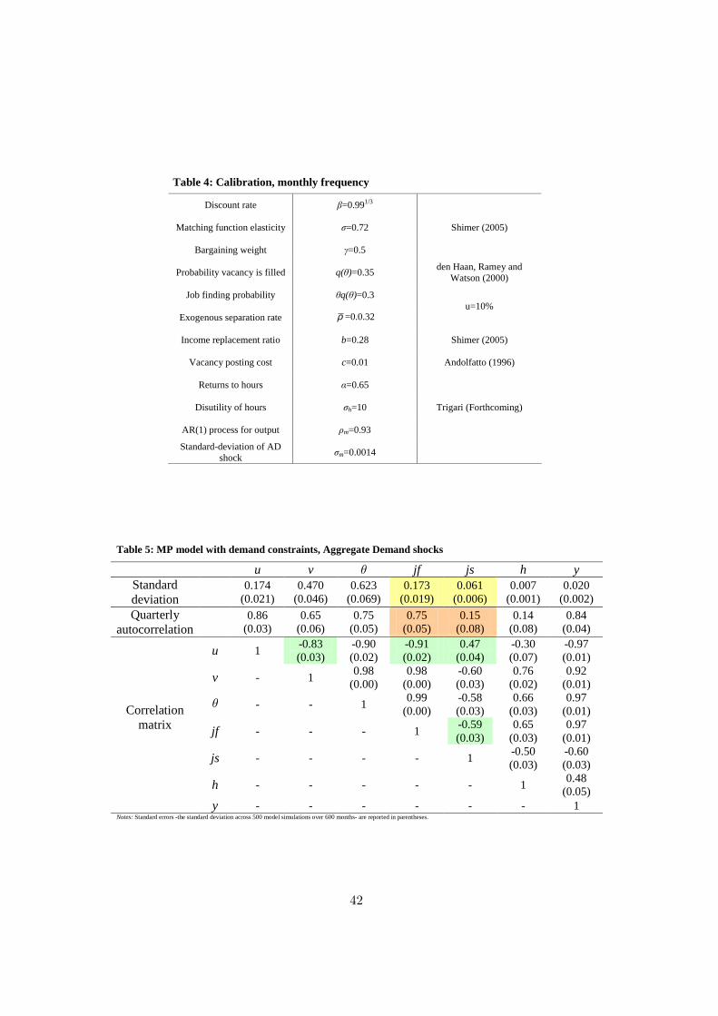
Table 4: Calibration, monthly frequency

Discount rate β=0.991/3

Matching function elasticity σ=0.72 Shimer (2005)

Bargaining weight γ=0.5

Probability vacancy is filled q(θ)=0.35 den Haan, Ramey andWatson (2000)

Job finding probability θq(θ)=0.3

Exogenous separation rate ρ =0.0.32u=10%

Income replacement ratio b=0.28 Shimer (2005)

Vacancy posting cost c=0.01 Andolfatto (1996)

Returns to hours α=0.65

Disutility of hours σh=10 Trigari (Forthcoming)

AR(1) process for output ρm=0.93

Standard­deviation of ADshock σm=0.0014

Table 5: MP model with demand constraints, Aggregate Demand shocks

u v µ jf js h yStandarddeviation

0.174(0.021)

0.470(0.046)

0.623(0.069)

0.173(0.019)

0.061(0.006)

0.007(0.001)

0.020(0.002)

Quarterlyautocorrelation

0.86(0.03)

0.65(0.06)

0.75(0.05)

0.75(0.05)

0.15(0.08)

0.14(0.08)

0.84(0.04)

u 1 ­0.83(0.03)

­0.90(0.02)

­0.91(0.02)

0.47(0.04)

­0.30(0.07)

­0.97(0.01)

v ­ 1 0.98(0.00)

0.98(0.00)

­0.60(0.03)

0.76(0.02)

0.92(0.01)

µ ­ ­ 1 0.99(0.00)

­0.58(0.03)

0.66(0.03)

0.97(0.01)

jf ­ ­ ­ 1 ­0.59(0.03)

0.65(0.03)

0.97(0.01)

js ­ ­ ­ ­ 1 ­0.50(0.03)

­0.60(0.03)

h ­ ­ ­ ­ ­ 1 0.48(0.05)

Correlationmatrix

y ­ ­ ­ ­ ­ ­ 1Notes: Standard errors ­the standard deviation across 500 model simulations over 600 months­ are reported in parentheses.

42

Table 6: Contribution of JF/JS and Skewness, model data

Size of AD shocks ¾ ½ ¾

Contribution of JS 22 %(0.03)

13 %(0.02)

Contribution of JF 78 %(0.03)

87 %(0.02)

Skewness(dU) 0.53**(0.16))

0.14(0.17))

Notes: u and y are monthly model unemployment and output. The contributions of JF and JS are calculated usingthe method from Shimer (2007) and Fujita and Ramey (2007). Standard errors ­the standard deviation across 500model simulations over 600 months (50 years)­ are reported in parentheses.

Figure 1: Empirical Cross-Correlograms of the Job Finding rate and the Job Separation ratewith Unemployment and Output over 1951-2006.

­8 ­6 ­4 ­2 0 2 4 6 8­1

­0.8­0.6­0.4­0.2

00.20.40.60.8

1

corr(JF,Ut+j)­8 ­6 ­4 ­2 0 2 4 6 8

­1­0.8­0.6­0.4­0.2

00.20.40.60.8

1

corr(JS,Ut+j)

­8 ­6 ­4 ­2 0 2 4 6 8­1

­0.8­0.6­0.4­0.2

00.20.40.60.8

1

corr(JF,Yt+j)­8 ­6 ­4 ­2 0 2 4 6 8

­1­0.8­0.6­0.4­0.2

00.20.40.60.8

1

corr(JS,Yt+j)

43

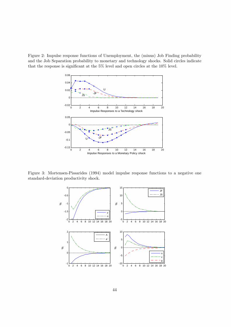
Figure 2: Impulse response functions of Unemployment, the (minus) Job Finding probabilityand the Job Separation probability to monetary and technology shocks. Solid circles indicatethat the response is signi�cant at the 5% level and open circles at the 10% level.

0 2 4 6 8 10 12 14 16 18 20­0.02

0

0.02

0.04

0.06

Impulse Responses to a Technology shock

0 2 4 6 8 10 12 14 16 18 20­0.15

­0.1

­0.05

0

0.05

Impulse Responses to a Monetary Policy shock

­JFJS

U

­JFU

JS

Figure 3: Mortensen-Pissarides (1994) model impulse response functions to a negative onestandard-deviation productivity shock.

0 2 4 6 8 10 12 14 16 18 20­2

­1.5

­1

­0.5

0

%

yn

0 2 4 6 8 10 12 14 16 18 20­5

0

5

10

15

%

JFJS

0 2 4 6 8 10 12 14 16 18 20­1

0

1

2

%

A

a~

0 2 4 6 8 10 12 14 16 18 20­10

­5

0

5

10

%

uvθ

44

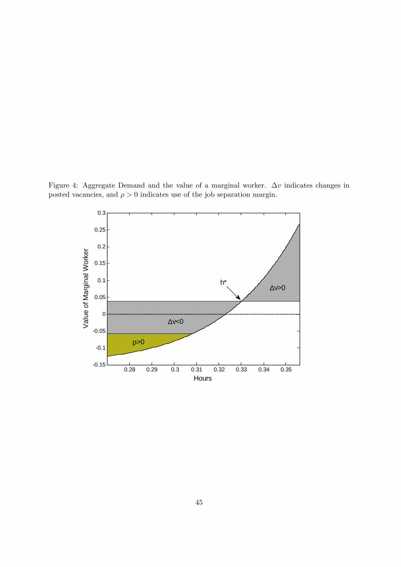
Figure 4: Aggregate Demand and the value of a marginal worker. �v indicates changes inposted vacancies, and � > 0 indicates use of the job separation margin.

0.28 0.29  0.3 0.31 0.32 0.33 0.34 0.35­0.15

­0.1

­0.05

0

0.05

0.1

0.15

0.2

0.25

0.3

ρ>0

∆v>0

∆v<0

Hours

Val

ue o

f Mar

gina

l Wor

ker

h*

45

Figure 5: Model impulse response functions to a positive one standard-deviation aggregatedemand shock.

0 2 4 6 8 10 12 14 16 18 20­0.2

­0.15

­0.1

­0.05

0

0.05

Unemployment

%

0 2 4 6 8 10 12 14 16 18 200

0.01

0.02

0.03

0.04

Hours per Worker

%

0 2 4 6 8 10 12 14 16 18 200

0.1

0.2

0.3

0.4

JF

%

0 2 4 6 8 10 12 14 16 18 20­1

­0.5

0

0.5

1

JS

%

Figure 6: Model impulse response functions to negative aggregate demand shocks with respec-tive size of one and one-half standard-deviation.

0 2 4 6 80

0.05

0.1

0.15

0.2

Unemployment

%

0 2 4 6 8­6

­4

­2

0

2x 10

­3

Hours per Worker

%

0 2 4 6 8­0.2

­0.15

­0.1

­0.05

0

JF

%

0 2 4 6 80

0.1

0.2

0.3

0.4

0.5

JS

%

1/2σy

σy

46

Figure 7: Model impulse response functions of gross hires to negative aggregate demand shocksof di¤erent size.

0 2 4 6 8 10 12 14 16 18 20­0.015

­0.01

­0.005

0

0.005

0.01

0.015

0.02

0.025

0.03

0.035

Gross Hires

0.5σy

1σ1.5σ

Figure 8: Model (plain line) and empirical (dotted line) cross-correlograms of the Job Findingrate and the Job Separation rate with Unemployment and Output.

­8 ­6 ­4 ­2 0 2 4 6 8­1

­0.8­0.6­0.4­0.2

00.20.40.60.8

1

corr(JF,Ut+j)­8 ­6 ­4 ­2 0 2 4 6 8

­1­0.8­0.6­0.4­0.2

00.20.40.60.8

1

corr(JS,Ut+j)

­8 ­6 ­4 ­2 0 2 4 6 8­1

­0.8­0.6­0.4­0.2

00.20.40.60.8

1

corr(JF,Yt+j)­8 ­6 ­4 ­2 0 2 4 6 8

­1­0.8­0.6­0.4­0.2

00.20.40.60.8

1

corr(JS,Yt+j)

47