demand curve shape - aeso€¦ · demand curve under long-run equilibrium conditions ... supply,...

Copyright © 2017 The Brattle Group, Inc.

Kathleen Spees David Luke Oates

Judy Chang Peter Cahill

Johannes Pfeifenberger Elliott Metzler

Demand Curve Shape

Demand Curve Working Group

O c tober 1 0 , 2 0 1 7

Dra f t M a ter ia l s f o r D i sc uss io n

P RE PARED FOR

P RE PARED BY

Preliminary Modeling Results and Scoping Questions

Draft Materials for Discussion

| brattle.com 1

Agenda

▀ Overview

▀ Modeling Approach

▀ Supply Curve Concepts

▀ Initial Results

▀ Next Steps


| brattle.com 2

Overview

  The AESO has asked us to provide analytical support to the Working Group as you develop a capacity market demand curve

  Our tasks are to:

▀ Assist the Working Group to understand the potential performance of demand curves under consideration, drawing on experience from other markets and analysis of Alberta’s unique situation (i.e. small market, coal retirements, transition from energy-only, possible seasonal construct)

▀ Provide modeling support to assess potential price and quantity volatility with each demand curve under long-run equilibrium conditions (approach for assessing questions on near-term, transitional conditions is being reviewed by AESO)

▀ Identify open questions from the group and answer them in upcoming meetings (see next steps for open questions gathered to date)

  We kick off that discussion today with a preliminary analysis of how other markets’ curves would perform in Alberta, a sketch of curves tuned to Alberta’s market size, and discussion of the supply curve


| brattle.com 3

Overview

Concept: “Tuned” Demand Curves   Preliminary analysis indicates that Alberta’s small market may require a proportionally wider demand curve to mitigate expected price and net supply variability

% of Reliability Requirement Reserve Margin (% UCAP) UCAP MW Preliminary Working Assumptions

~3,000 - 4,000 MW Range

Standard deviation in

clearing prices ranges

between 25% and

45% of Net CONE

Tuned, Cap at 2× Net CONE

Tuned, Cap at 1.5× Net CONE


Target: 100 MWh/year EUE (Preliminary Working Assumption)

Minimum Acceptable:

800 MWh/year EUE

(Preliminary Working

Assumption)

“Tuned” Demand Curves

• Capacity markets will have year-to-year variability in supply and demand

• Other markets developed demand curves “tuned” to achieve the reliability requirement on average (though reliability varies from year to year)

• Applying that approach to Alberta, curves such as these would achieve 100 MWh/year EUE


| brattle.com 4

Agenda

▀ Overview



▀ Initial Results

▀ Next Steps


| brattle.com 5

Modeling Approach

Recap: Overview of Modeling Approach

  Primary Model Results

▀ Estimate average, range, and distribution of capacity market outcomes

− Price, quantity, and reliability

− Across annual or summer/winter auctions

▀ Summarize results realized with different demand curve shapes

  Approach

▀ Incorporate annual or seasonal supply and demand curves

▀ Clear supply and demand to calculate prices and quantities in the auction

▀ Simulate a distribution of outcomes using a Monte Carlo analysis of realistic “shocks” to supply, demand, and imports

▀ Average price over all draws must equal Net CONE, consistent with a market that supports entry at long-run marginal cost

Range of Price

Outcomes

Supply and Demand Shocks (Illustrative)

Supply Shocks

Demand Shocks

Range of Quantity Outcomes

Net CONE


| brattle.com 6

Modeling Approach

Supply Modeling

  Supply curves consist of three components

▀ Shape Blocks − Supply offers at prices above zero

− Shape based on historical PJM offer curves

− Scaled to total MW offers, which vary based on annual vs. summer/winter auction type

− Independent of demand curve shape

▀ Shock Block − Zero-priced supply block

− Quantity varies with each draw to generate “shocks” to the supply curve

− Represents expected year-to-year variability

▀ Smart Block − Zero-priced supply block

− Quantity adjusted such that the average price across all draws equals Net CONE

− Quantity is constant across draws, but may be slightly different across demand curves

Smart Block

Shock Block

Shape Block

Supply Curve Components (Illustrative)


| brattle.com 7


Minimum Acceptable:

800 MWh/year EUE


Assumption)

Modeling Approach

Demand and Reliability Modeling

  Demand Curves

▀ Arbitrary number of price-quantity pairs

▀ Quantities are relative to the reliability requirement

▀ Prices expressed as % of Net CONE

  Reliability

▀ Simulation reliability results are evaluated with respect to expected unserved energy (EUE) and a working assumption for reliability target

▀ EUE curve and target will be updated as new information becomes available

▀ Using quantity outputs, the EUE is tabulated over all simulation draws to estimate weighted-average reliability outcomes

Demand Curve and Reliability (Illustrative)

EUE Curve

Preliminary Working Assumption


| brattle.com 8

Modeling Approach

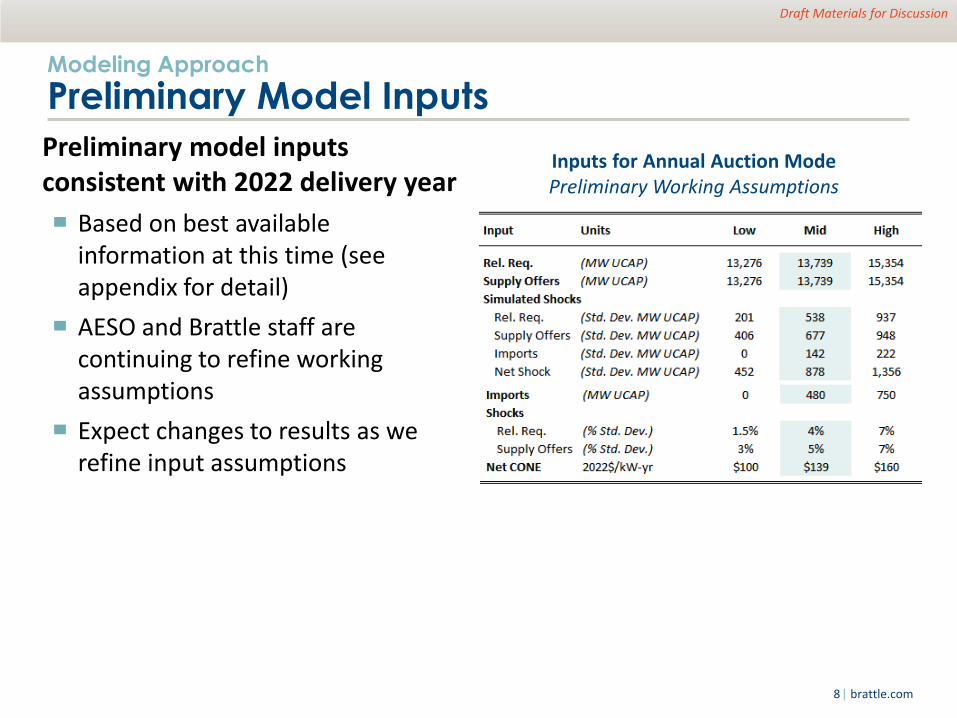
Preliminary Model Inputs

  Preliminary model inputs consistent with 2022 delivery year

▀ Based on best available information at this time (see appendix for detail)

▀ AESO and Brattle staff are continuing to refine working assumptions

▀ Expect changes to results as we refine input assumptions

Inputs for Annual Auction Mode Preliminary Working Assumptions


| brattle.com 9

Agenda

▀ Overview



▀ Initial Results

▀ Next Steps


| brattle.com 10

Supply Curve

How Do Sellers Offer in Other Markets?   In other forward capacity markets, approximately 70-85% of suppliers offer at a price of zero. Prices are set by the subset of above-zero offers

ISO-NE and PJM Three-Year Forward Markets

PJM Three-Year Forward and MISO Non-Forward Market

ISO New England

Sources: Pfeifenberger et al. “Third Triennial Review of PJM’s Variable Resource Requirement Curve” (2014) Testimony of Dr. Samuel A. Newell and Dr. Kathleen Spees on Behalf of ISO New England Inc. Regarding a Forward Capacity Market Demand Curve (2014) Testimony of Dr. Samuel A. Newell, Dr. Kathleen Spees, and Dr. David Luke Oates on Behalf of Midcontinent Independent System Operator (MISO).

PJM Range of Clearing Prices 2015/16-20/21

Clearing More Than 25,000 MW of New Generation

Supply Curves Affected by the Mercury & Air Toxics Standard

Many Coal Plants Faced Retire-or-Retrofit Decision at Once


| brattle.com 11

Supply Curve

What Drives the Offer Prices?

In a uniform price auction, the competitive offer price is at the minimum payment needed to break even for operating one more year. Over the lifecycle of a typical plant that translates to offers at:

▀ First Delivery Year: Offer at above-zero prices, consistent with investment costs minus expected net E&AS revenue (i.e. at Net CONE)

▀ Years 2+: Offer near zero. Energy market net revenues exceed going-forward fixed costs to stay in operation (plant will stay online even without capacity payments). The majority of plants fall into this category

▀ Aging Plant Needing Refurbishment: Offer at above-zero prices. Will retire or mothball if capacity price is too low to recover re-investment costs

Offer Price* = Going-Forward Fixed Costs − Expected E&AS Net Revenue

Notes: *Many other complexities affect offer prices, including opportunity costs, penalty and obligation costs under the capacity market, and the expected trajectory of

energy and capacity prices in years 2+. This simplified discussion covers only the largest drivers of offer prices for traditional thermal generating resources.


| brattle.com 12

Agenda

▀ Overview



▀ Initial Results

▀ Next Steps


| brattle.com 13

Initial Results

Tested Demand Curves

  Tested several demand curves for performance if translated to Alberta’s context. Compared:

▀ Vertical curve

▀ PJM, ISO-NE, and NYISO curves

▀ “Tuned” straight-line curves with price caps 1.5× to 2× Net CONE, and foot point adjusted until reliability is at the target

Demand Curves Tested

Tuned, Cap at 2× Net CONE

NYISO

ISO-NE

PJM



% of Reliability Requirement Reserve Margin (% UCAP) UCAP MW


Minimum Acceptable:

800 MWh/year EUE


Assumption)

Preliminary Working Assumptions


| brattle.com 14

Initial Results

Histogram Results (PJM Curve)

  When applied to AESO, PJM’s demand curve results in a significant number of auctions with prices at the cap and low reliability

Prices Quantities

Prices often at the administrative cap, high price volatility

Quantities often below the minimum

acceptable threshold


Minimum Acceptable:

800 MWh/year EUE


Assumption)


| brattle.com 15

Initial Results

Preliminary Results: Demand Curve Performance

  Initial results indicate that Alberta may need a proportionally wider/flatter demand curve than those used in other markets to mitigate price volatility and reliability in the smaller market

Model Simulation Results for Selected Demand Curves

The existing RTO and vertical curves

support reliability far below the target

Average prices equal Net CONE with all curves

Existing RTO and vertical curves fall short of the

requirement about 1/3 to 1/2 of the time

The tuned curves achieve target

reliability at 100 MWh/year EUE

Vertical curve produces high price volatility


| brattle.com 16

Agenda

▀ Overview



▀ Initial Results

▀ Next Steps


| brattle.com 17

Next Steps

Questions from the Working Group

  Brattle and AESO are seeking input from the workgroup to guide further demand curves or sensitivities to evaluate. Building on discussion from the last meeting, potential questions include:

▀ How sensitive are “tuned” curves to supply/demand shocks, reliability requirement, and supply curve shapes?

▀ What’s the equilibrium MW of supply compared to current, and how long would it take Alberta to reach equilibrium with each demand curve?

▀ What supply curve sensitivities make sense to test for the specific Alberta context (e.g. existing suppliers offer at 50% of Net CONE)?

▀ How should the Working Group think about the demand curve in the context of a seasonal auction?

▀ How should the demand curves reflect incremental reliability benefits and the value of lost load?

▀ Additional questions identified in this meeting or submitted offline


| brattle.com 18

Next Steps

Timing Scope

SAM 2.0-3.0 Sept-Dec 2017

Oct 4 Web/Phone Meeting

Gather feedback from workgroup on scope

Oct 10 In-Person Meeting (Today):

Discuss preliminary analysis of potential demand curve shapes Review Alberta-specific considerations affecting price volatility and desirable curve width/parameters Expand on and complement introduction of demand curve concepts/principles by providing information on

modeling approach, impacts of key parameters and principles, preliminary suggestions about the “workable range” of demand curve parameters

Nov 1 Meeting:

Develop materials in response to workgroup questions, requested sensitivity analysis, and requested demand curve alternatives. Provide 2-4 workable demand curve options for the workgroup to consider for SAM 3.0

Nov 15 Meeting:

Respond to workgroup questions/input. Discuss demand curve selected for SAM 3.0, finalize principles

SAM 3.0-4.0 Jan-Mar 2018

Jan Meeting: Outline outstanding uncertainties/questions to be refined in SAM 4.0, primary interactions/uncertainties, gather stakeholder input on necessary refinements

Feb or Mar Meeting: Answer outstanding questions, finalize demand curve parameters. Develop workgroup conclusion for SAM 4.0 demand curve parameters

SAM 4.0-5.0 Apr-Jun 2018

Make final adjustments to demand curve based on final AESO/workgroup input and conforming changes to other workgroups’ changes in SAM 4.0

April Meeting: Provide final presentation to the workgroup on selected demand curve and recommendations to be included in report. Last opportunity for stakeholder input/adjustments

June Recommendations Report/Testimony: Prepare final recommendations report and deliver to workgroup/AESO. Document the defined objectives, principles, workgroup process, and dissention. Include final recommended Demand Curve. Submit report or testimony suitable for filing with governing body


| brattle.com 19

Contact Information

The views expressed in this presentation are strictly those of the presenter(s) and do not necessarily state or reflect the views of The Brattle Group, Inc.

DAVID LUKE OATES Associate │ Boston, MA [email protected] +1.617.234.5212

KATHLEEN SPEES Principal│ Boston, MA [email protected] +1.617.234.5783

JOHANNES PFEIFENBERGER Principal │ Boston, MA [email protected] +1.617.234.5624

JUDY CHANG Principal and Director │ Boston, MA [email protected] +1.617.234.5630


| brattle.com 20

About The Brattle Group

The Brattle Group provides consulting and expert testimony in economics, finance, and regulation to corporations, law firms, and governmental agencies worldwide.

We combine in-depth industry experience and rigorous analyses to help clients answer complex economic and financial questions in litigation and regulation, develop strategies for changing markets, and make critical business decisions.

Our services to the electric power industry include:

▀ Climate Change Policy and Planning

▀ Cost of Capital

▀ Demand Forecasting Methodology

▀ Demand Response and Energy Efficiency

▀ Electricity Market Modeling

▀ Energy Asset Valuation

▀ Energy Contract Litigation

▀ Environmental Compliance

▀ Fuel and Power Procurement

▀ Incentive Regulation

▀ Rate Design and Cost Allocation

▀ Regulatory Strategy and Litigation Support

▀ Renewables

▀ Resource Planning

▀ Retail Access and Restructuring

▀ Risk Management

▀ Market-Based Rates

▀ Market Design and Competitive Analysis

▀ Mergers and Acquisitions

▀ Transmission


| brattle.com 21

Offices

BOSTON NEW YORK SAN FRANCISCO

WASHINGTON, DC TORONTO LONDON

MADRID ROME SYDNEY


| brattle.com 22

Appendix Model Input Details


| brattle.com 23

Appendix

Supply Shocks

  Applied to supply curves to capture real world variability in offered supply quantities

▀ Evaluated year-to-year variability in supply offers in similar-sized zones within PJM, MISO, and ISO-NE

− Standard deviations range 3%-7%

− Recommended mid-point of 5%

Standard Deviation in Offered Supply

Regions the Size of Alberta


| brattle.com 24

Appendix

Demand Shocks

  Applied to reliability requirement to account for expected variability in demand

▀ Based on variability in AESO load forecasts 3 to 4 years out

▀ Supplemented based on variability in reliability requirements for other markets’ capacity zones the same size as Alberta

▀ Recommend 4% standard deviation as the midpoint, and 1.5%-7% sensitivity range

Historical Peak Load Forecast by Forecast Year

Year-to-Year Variability in Demand in Comparably Sized Zones

demand curve shape - aeso€¦ · demand curve under long-run equilibrium conditions ... supply,...

Documents