demand bubbles and phantom orders in supply chains

Demand Bubbles and Phantom Orders in Supply Chains

by

Paulo M. Gonçalves

Bachelor of Science, Mechanical Engineering (1992) Instituto Tecnológico de Aeronáutica

Master of Science, Energy Planning (1995)

Universidade de São Paulo

Master of Science, Technology and Policy (1998) Massachusetts Institute of Technology

Submitted to the Alfred P. Sloan School of Management in partial fulfillment of the requirements for the degree of

Doctor of Philosophy in Management

at the

Massachusetts Institute of Technology

June 2003

2003 Massachusetts Institute of Technology All Rights Reserved

Signature of Author: ______________________________________________________ Sloan School of Management

May 2003

Certified by: _____________________________________________________________

John D. Sterman Professor of Management Science

Thesis Supervisor

Accepted by: ____________________________________________________________ Birger Wernerfelt

Chairman, Ph.D. Committee Sloan School of Management

3

Demand Bubbles and Phantom Orders in Supply Chains

by

Paulo M. Gonçalves

Submitted to the Alfred P. Sloan School of Management in May 2003 in partial fulfillment of the requirements for the degree of

Doctor of Philosophy in Management

ABSTRACT

Essay One The Impact of Shortages on Push-Pull Production Systems

This paper explores the impact of endogenous customer demand on supply chain instability. It investigates how a semiconductor manufacturer’s hybrid push-pull production system responds to customer demand, when inventory availability influences demand. While customers’ response to variable service level represents an important concern in industry with sizable impacts on company profitability, previous models exploring supply chain instability do not address it. This research incorporates customer response in two important ways. First, a negative feedback loop of lost sales captures the effect that an initial increase (decrease) in demand leads to a decrease (increase) in the manufacturer’s service level, causing customer demand to decrease (increase). Second, a positive feedback loop of production push characterizes the manufacturer increase (decrease) in capacity utilization to respond to a surge (drop) in demand, leading to high (low) production volumes and service levels, and a further increase (decrease) in demand.

The manufacturer’s hybrid push-pull production system is very effective in meeting customer demand. Stockouts at different stages in the supply chain, however, can shift the operation mode of the system to a de facto push system. The shift to a push system decreases the manufacturers’ service level and increases demand variability. The analysis suggests that the endogenous customer demand assumption influences the shifts in modes of operation through the lost sales and production push loops, leading to higher supply chain instability than when customer demand is modeled as exogenous. In addition, incorporating the endogenous demand assumption leads to a different inventory and utilization policies than the ones currently adopted. First, this research finds that supply chains can operate in multiple modes, due to demand instability. It also provides policies capable of mitigating the impact from shifts in operation modes. Second, it suggests that models investigating instability in supply chains assuming exogenous demand may underestimate the amplification in demand and the value of inventory buffers. The model analyzed in this paper gives insights into the costs of lean inventory strategies in the context of hybrid production systems.

4

Essay Two Why do Shortages Inflate to Huge Bubbles? When demand exceeds supply, customers often hedge against shortages by placing multiple orders with multiple suppliers. The resulting demand bubble creates instability leading to excess capacity, excess inventory, low capacity utilization, and financial and reputation losses for suppliers and customers. This paper contributes to the understanding of demand bubbles caused by shortages by providing a comprehensive causal map of supplier-customer relationships and a formal mathematical model of a subset of those relationships. It provides closed form solutions for supply chain dynamics when supplier capacity is fixed and simulation analysis when it is flexible. Sensitivity analysis provides a deeper understanding of structures and decision rules that contribute to bubbles and suggests policies for improvement. For instance, the ability to quickly build capacity can reduce bubble size. In addition, the time it takes customers to perceive and to react to supply availability is an important lever in controlling demand bubbles. While longer customer perception delays of supply availability stabilize the entire supply chain, it counters conventional wisdom and IT spending on real-time information systems and it can be harmful to individual customers. Essay Three Investigating the Causes of Returns in the Seed Supply Chain Hoarding is a common occurrence during shortages of “hot” products in industries ranging from oil to toys to computers to pharmaceuticals. Often the induced shortage due to hoarding is much stronger than the original trigger. This paper investigates the impact of dealer hoarding on generating large amounts of seeds returned to a seed corn supplier in the agribusiness industry. To understand the mechanisms leading to seed corn hoarding and returns, we build a formal model of seed hoarding in the agribusiness supply chain. Our insights suggest that dealer hoarding and subsequent seed returns result from the interplay between supply chain characteristics (e.g. timing of information availability and quality of dealers’ orders) and human decision making (e.g. salespeople’ s effort allocation decisions and managers’ pressure). In addition, a number of supplier actions can intensify dealers hoarding behavior, worsening the problem. Our analysis suggests several policies capable of effectively reducing the volume of returns. Thesis Supervisor: John D. Sterman Title: Professor of Management Science

5

Acknowledgements While it has not been easy to write this thesis, I have enjoyed it. This research reflects to a large extent the diverse set of talents of the people involved with it. The quality of the work benefited enormously from the perspectives and contribution of the members on my thesis committee. I am honored to have worked with them. From the beginning, Charlie Fine urged me to narrow the problem focus and sharpen my views. Along the process, he provided many valuable comments and insights, constructively challenging my assumptions and results. I am very grateful for his contributions. Gabriel Bitran took time away from his busy schedule as deputy dean of Sloan to work with me. He helped me bridge the gap from system dynamics to operations management while providing valuable feedback on “big picture” issues. It was a privilege to work with him. The third essay would not have been possible without the support of Jim Rice. He opened the doors to a research site and helped me put in perspective how my research mattered in the real world. Jim also provided expert guidance in how to manage the thesis process and, more importantly, always provided a word of friendship and advice throughout the process. Jim Hines advised me through my master thesis, taught me a lot about modeling, and read through numerous early drafts of my work. He instilled in me a passion for being helpful, curious, and always seeking insight. Jim nurtured me in the early stages of my research, providing clear direction, sound advice, and making research enjoyable with his great sense of humor. The first essay benefited immensely from Jim’ s work. I owe my introduction to system dynamics and my admission to the doctoral program to John Sterman. Both opportunities have transformed my life, and for that I am eternally grateful. John played a crucial role in my academic development as a teacher, mentor, and friend. He has shaped every aspect of the thesis and has already motivated future research. I truly enjoyed having the opportunity to work with him and hope that our collaboration will continue in the coming years. Many people, in two different field sites, generously gave their time and shared their expertise. I gratefully acknowledge their essential help. At Intel, I acknowledge the contribution of Dave Fanger, Jay Hopman, Ann Johnson, George Brown, Gordon McMillan, and Jim Kellso. I offer a special thanks to Mary Murphy-Hoye who has embraced system dynamics and has supported the research effort with countless efforts. Mary has contributed to the research in more ways that is possible to describe. At the other research site, I thank to Garth Blanchard and Jon Nienas for giving me the opportunity to work with them and making the research possible. Special thanks to Kurt Rahe for his patience and effort to study my models and understand their implicit assumptions and resulting behavior. Even before entering the doctoral program, Hank Taylor made me feel part of the SD family. Scott Rockart and Liz Keating, as expert doctoral students, were very friendly and helpful in guiding me through classes, foundation and breadth courses, and general exams. Together

6

with Rogelio Oliva, Nitin Joglekar, and Ed Anderson they became good friends and a constant source of support and good advice. I shared a small office with Laura Black for many years and despite the lack of space and intense pressure, we became close friends. I cherish the support we provided each other in the most difficult times through the program. Laura has read many early drafts of my research proposal and encouraged me to be a thoughtful researcher. More importantly, Laura has helped me find my own voice. Brad Morrison also became a good friend in the program and was a constant source of experience and advice. His unique insights and perspectives always surprised and amazed me. I was fortunate to share many of Mila Getmansky’ s achievements. In many ways, we matured together through the program. I am happy to have had that opportunity. Together with Laura, Brad, and Mila, I have shared many good times with my friends Hazhir Rahmandad, Jeroen Struben, and Gokhan Dogan. They were a constant source of encouragement and friendship, and they provided the doctoral program with a distinctive character, that I will forever cherish. Charlie Lertpattarapong participated in the interviews and modeling of the first essay. Charlie made the work fun and enjoyable. I made several good friends at the OM program. Juan Carlos Ferrer always cheered me on in difficult times. He taught me by remarkable example to always have a positive attitude despite adversities. I am deeply grateful for his friendship. Paulo Oliveira has traced a parallel path to mine during his doctoral studies as a good friend and fellow countryman. Paulo has constantly reminded me of the treasures of our heritage and our people. Felipe Caro, Opher Baron, and Hasan Arslan were great friends. They provided valuable feedback and a strong sense of community. I was first exposed to academic research at MIT through Nelson Repenning. I thank him for his efforts in preparing me for thesis research as well as his coaching regarding presenting my findings. Anjali Sastry took an interest in my work, when she came to MIT and has since helped me with her thoughtful comments. I only met JoAnne Yates in my last year in the program but I left with a profound admiration for her respect for people. I am indebted to Jay Forrester for his pioneering work in creating system dynamics, and I truly admire his courage and his sense of purpose. I would also like to thank my family. My grandmother’ s words of encouragement instilled in me a sense of hope and perseverance. My father always supported me in my pursuit of my dreams and motivated me from an early age to excel in my studies. My brothers have been kind and constant friends despite the distance. I am also thankful to Flávia’ s family. Their excitement and encouragement have been a motivating force throughout the years. Above all, I would like to thank my wife, Flávia Gonçalves. She has been a caring and devoted wife, and has rewarded me with relentless and unconditional love. She has never doubted that I could do it, even when my own trust faded. Her continuous trust and support were a guiding force in this journey. I dedicate this thesis to her as a token of appreciation for all her support.

7

To Flávia

9

Table of Contents Essay One THE IMPACT OF SHORTAGES ON PUSH-PULL PRODUCTION SYSTEMS ABSTRACT...........................................................................................................................................................11

1. INTRODUCTION........................................................................................................................................... 13 2. LITERATURE REVIEW............................................................................................................................... 17 3. MODEL ASSUMPTIONS AND STRUCTURE........................................................................................... 22

3.1. MODEL ASSUMPTIONS................................................................................................................................ 23 3.1.1. Capacity Utilization........................................................................................................................... 23 3.1.2. Demand forecasting........................................................................................................................... 24 3.1.3. Inventory management....................................................................................................................... 25 3.1.4. Customer response ............................................................................................................................ 28

3.2. MODEL STRUCTURE ................................................................................................................................... 30 4. MODEL ANALYSIS AND RESULTS.......................................................................................................... 32

4.1. SENSITIVITY ANALYSIS .............................................................................................................................. 36 4.1.1. Sensitivity to Capacity Utilization ..................................................................................................... 37 4.1.2. Sensitivity to Customer Response ...................................................................................................... 39

4.2. MODES OF BEHAVIOR ................................................................................................................................. 41 Behavior ...................................................................................................................................................... 45

4.3. EIGENVALUE ELASTICITY........................................................................................................................... 46 4.3.1. Phase-One Analysis ........................................................................................................................... 49 4.3.2. Phase-Two Analysis........................................................................................................................... 51 4.3.3. Phase-Three Analysis ........................................................................................................................ 53 4.3.4. Summary: Eigenvalue Elasticity Analysis ......................................................................................... 55

4.4. POLICY DISCUSSION.................................................................................................................................... 58 5. DISCUSSION AND DIRECTIONS FOR FUTURE RESEARCH............................................................. 59 7. REFERENCES................................................................................................................................................ 65 APPENDIX A: PURE PUSH, PURE PULL, AND HYBRID PUSH-PULL SYSTEMS............................... 69

B.1. MANUFACTURING PROCESS....................................................................................................................... 72 B.2. PRODUCTION AND INVENTORY CONTROL.................................................................................................. 73

B.2.1. Production Push................................................................................................................................ 73 B.2.2. Demand Pull...................................................................................................................................... 77

B.3. DISTRIBUTION AND LOGISTICS .................................................................................................................. 81 APPENDIX C: EIGENVALUE ELASTICITY TABLES ............................................................................... 86

Essay Two WHY DO SHORTAGES INFLATE TO HUGE BUBBLES? ABSTRACT...........................................................................................................................................................89

1. MOTIVATION................................................................................................................................................ 91

10

2. LITERATURE REVIEW............................................................................................................................... 95 3. POSITIVE FEEDBACKS IN SUPPLY CHAINS ........................................................................................ 98 4. THE MODEL ................................................................................................................................................ 102 5. MODEL ANALYSIS .................................................................................................................................... 108

5.1. FIXED SUPPLIER CAPACITY ...................................................................................................................... 108 5.2. VARIABLE SUPPLIER CAPACITY ............................................................................................................... 116 5.3. PARAMETRIC SENSITIVITY ANALYSIS ...................................................................................................... 119

5.3.1. Time to build capacity ( Kτ ) ............................................................................................................ 120 5.3.2. Time for Customers’ to Perceive Delivery Delay ............................................................................ 121 5.3.3. Customers’ reactions to delivery delay............................................................................................ 124

5.4. MULTIVARIATE SENSITIVITY ANALYSIS................................................................................................... 126 5.5. OPTIMAL CAPACITY TRAJECTORY............................................................................................................ 128 5.6. OPTIMAL CONTROL POLICY ..................................................................................................................... 131

6. DISCUSSION ................................................................................................................................................ 134 7. REFERENCES.............................................................................................................................................. 138

Essay Three INVESTIGATING THE CAUSES OF RETURNS IN THE SEED SUPPLY CHAIN ABSTRACT..........................................................................................................................................................143

1. INTRODUCTION......................................................................................................................................... 145 2. SEED SUPPLY CHAIN ............................................................................................................................... 148 3. MODEL STRUCTURE AND ASSUMPTIONS......................................................................................... 151

3.1. MANAGERS’ PRESSURE ON SALESPEOPLE ................................................................................................ 155 3.2. SALESPEOPLE’ S EFFORT ALLOCATION ..................................................................................................... 157 3.3. DEALERS’ DESIRED ORDERS .................................................................................................................... 159 3.4. SUPPLIER’ S PRODUCTION RATE ............................................................................................................... 161

4. MODEL ANALYSIS .................................................................................................................................... 162 4.1. BASE CASE ............................................................................................................................................... 162 4.2. SENSITIVITY ANALYSIS............................................................................................................................. 165

4.2.1 Sensitivity to Pressure on Salespeople’ s Effort Allocation ............................................................... 165 4.2.1 Sensitivity to Position Effort on Probability ..................................................................................... 167

4.3. THE CASE FOR SENDING SEEDS EARLY ...................................................................................................... 169 5. POLICY ANALYSIS .................................................................................................................................... 171

5.1. ORDER PACING POLICY ............................................................................................................................ 172 5.2. FISCAL YEAR POLICY ................................................................................................................................ 173 5.3. SALESPEOPLE’ S PLAYBOOK POLICY.......................................................................................................... 173 5.4. EARLY SHIP POLICY .................................................................................................................................. 175

6. DISCUSSION ................................................................................................................................................ 176 7. REFERENCES.............................................................................................................................................. 183 APPENDIX A: MODEL DESCRIPTION ...................................................................................................... 185

11

The Impact of Shortages on Push-Pull Production Systems

Paulo Gonçalves

Sloan School of Management Massachusetts Institute of Technology

Operations Management / System Dynamics Group Cambridge, MA 02142

[email protected]

Abstract: This research explores the impact of endogenous customer demand on supply chain

instability. It investigates how a semiconductor manufacturer’ s hybrid push-pull production system responds to customer demand, when inventory availability influences demand. While customers’ response to variable service level represents an important concern in industry with sizable impacts on company profitability, previous models exploring supply chain instability do not address it. This research incorporates customer response in two important ways. First, a negative feedback loop of lost sales captures the effect that an initial increase (decrease) in demand leads to a decrease (increase) in the manufacturer’ s service level, causing customer demand to decrease (increase). Second, a positive feedback loop of production push characterizes the manufacturer increase (decrease) in capacity utilization to respond to a surge (drop) in demand, leading to high (low) production volumes and service levels, and a further increase (decrease) in demand.

The manufacturer’ s hybrid push-pull production system is very effective in meeting customer demand. Stockouts at different stages in the supply chain, however, can shift the operation mode of the system to a de facto push system. The shift to a push system decreases the manufacturers’ service level and increases demand variability. The analysis suggests that the endogenous customer demand assumption influences the shifts in modes of operation through the lost sales and production push loops, leading to higher supply chain instability than when customer demand is modeled as exogenous. In addition, incorporating the endogenous demand assumption leads to a different inventory and utilization policies than the ones currently adopted. First, this research finds that supply chains can operate in multiple modes, due to demand instability. It also provides policies capable of mitigating the impact from shifts in operation modes. Second, it suggests that models investigating instability in supply chains assuming exogenous demand may underestimate the amplification in demand and the value of inventory buffers. The model analyzed in this paper gives insights into the costs of lean inventory strategies in the context of hybrid production systems.

Keywords:

Supply chain management, push-pull systems, demand amplification, lost sales, endogenous demand, eigenvalue analysis, system dynamics, and simulation.

13

1. Introduction

Companies in diverse industries such as computers, autos, toys, and pharmaceuticals

struggle with supply chain instability. This struggle is particularly acute for semiconductor

manufacturers: Intel Corporation, the main U.S. semiconductor manufacturer, has consistently

faced oscillations in customer demand, inventories, and capacity utilization. Even though Intel

normally operates at high capacity utilization (above an 85% normal operating target), they

experience periods of low utilization almost every year. The variability in aggregate

utilization can reach up to 30% (Figure 1).1 In addition, the variability in any individual

facility is much higher. Since fabrication facilities (fabs) cost on average $2 billion, the costs

associated with instability in utilization are significant.

Year 1 Year 3 Year 5 Year 7

Cap

acit

y U

tiliz

atio

n

(All

faci

litie

s)

30%

Year 1 Year 3 Year 5 Year 7

Cap

acit

y U

tiliz

atio

n

(All

faci

litie

s)

Year 1 Year 3 Year 5 Year 7Year 1 Year 3 Year 5 Year 7

Cap

acit

y U

tiliz

atio

n

(All

faci

litie

s)

30%

Figure 1. Capacity Utilization at Intel across all facilities

Furthermore, oscillations in capacity utilization can lead to uneven supply and poor

profitability. Capacity utilization instability can be intensified by the long throughput time –

1 The scale for the y-axis is missing to protect Intel’ s confidentiality.

14

approximately 13 weeks – associated with wafer fabrication. The long fabrication throughput

time affects the ability of semiconductor manufacturers to replenish inventories in response to

changes in demand. When customer demand is strong, factory managers may operate at high

capacity utilization to keep inventory levels high throughout the supply chain; when customer

demand is weak, managers may reduce utilization, to avoid inventory gluts across the chain.

Variability in capacity utilization will have an impact on downstream inventory levels (e.g., at

assembly and finished goods) after the long fabrication delay. The combination of variability

in utilization and long fabrication delays can causes Intel (and other semiconductor

manufacturers) to experience times of scarce supply as well as times of excess supply. More

importantly, this variability in supply influences customer demand and profitability as Intel’ s

inability to meet demand may lead to lost sales and potentially loss of goodwill. For instance,

“Gateway Inc. said it will increase the number of microprocessors it buys from Advanced

Micro Devices Inc. to offset Intel's inability to match rising demand” (Hachman 2000). A

supply operations manager at Intel also acknowledges the problem: “If Intel does not have the

part, customers will tentatively work with us ... but if they cannot get it, they will go to AMD”

(Gonçalves 2002c). In addition, Intel’ s variability in supply can reduce its profitability. In

December 1998, Intel struggled with shortages of its low-end Celeron microprocessors,

allowing AMD, Intel’ s main competitor in the U.S market, to increase its market segment

share by more than two percentage points, even after Intel cut prices on its Celeron chips

(Hachman 1999).

Managers often explain their inability to meet customer demand by adopting an

exogenous point of view, citing reasons such as an unexpected increase in customer demand

during shortages or a softening of demand during excesses. In December 1999, Intel was

15

again struck by a major shortage of microprocessors. The company was unable to fill new

orders and declared that it would not be able to catch up with the backlog until later in the

following quarter. When asked for the reasons behind the shortage, an Intel manager

suggested that “ Demand was very high for Christmas. We came out of Q4 with lean

inventory, and demand has continued to be high" (Souza 2000). In his article reporting the

event, Souza (2000) notes that the explanation fails to take into account “ the historical pattern

of a first-quarter letdown.”

The interaction of supply chain instability and customer response faced by Intel raise

several interesting questions: What is the impact of endogenous demand on supply chain

variability? What are the impacts of supply chain instability to the supply chain operation?

What are the causes of oscillation in capacity utilization, leading to supply excesses and

shortages? Can Intel implement policies capable of stabilizing the system?

To address these questions, this research builds and analyzes a stylized model of a

semiconductor manufacturer supply chain, in which customer demand responds to product

availability. The modeling effort draws on a year-long, in-depth study of Intel’ s supply chain.

Microprocessor fabrication at Intel takes place in a hybrid push-pull production system

in a three stage supply chain consisting of fabrication, assembly, and distribution. In addition

to the material flows of production, the model captures the customers’ response to the

manufacturer’ s service level. In particular, it incorporates two feedback loops that are

important in practice, but are often not incorporated in supply chain models. First, a negative

feedback loop of lost sales captures the effect that an initial increase (decrease) in demand

leads to a decrease (increase) in the manufacturer’ s service level, causing customer demand to

decrease (increase). Hence, in the lost sales loop a decrease (increase) in demand generates a

16

reaction that balances the impact of the initial disturbance. Second, a positive feedback loop

of production push characterizes the manufacturer’ s increase in capacity utilization to respond

to a surge in demand. As production volume increases, the manufacturer is able to maintain a

higher service level, leading to an increase in customer demand. In the production push loop

the system reaction tends to reinforce the impact of the original disturbance.

This work contributes to the literature by introducing a novel method of analysis. The

research relies not only on simulation, the traditional approach to investigate the behavior of

systems of nonlinear ordinary differential equations, but also on eigenvalue elasticity theory

(Forrester 1982, 1983; Kampmann 1996; Gonçalves et al. 2000) to analyze the model and

derive the main insights.

Through the eigenvalue analysis, it is possible to understand the behavior of the

nonlinear system as composed by the behavior of three (quasi) linear systems. In particular,

the analysis concludes that the semiconductor manufacturer supply chain can experience

shifts in the mode of operation, moving from a hybrid push-pull system to a pure push system.

This takes place due to stock-outs in different stages of the supply chain. For instance, if Intel

stocks out of finished goods inventory, it will not be able to “ pull” such products. Instead, it

will push the products as they become available from assembly. The departure of the system

operation from its original design as a hybrid push-pull system to a push system leads to

increased variability in demand and decreased firm performance. In addition, the endogenous

customer demand assumption influences the shifts in modes of operation through the lost

sales and production push loops, leading to higher supply chain instability than when

customer demand is exogenous. Moreover, the endogenous demand assumption leads to a

different inventory and utilization policies than the ones currently adopted. The policies

17

recommended by the analysis suggests that the supplier (1) maintains higher inventory buffers

in assembly WIP and finished goods, (2) reduces utilization responsiveness to changes in

customer demand, and (3) maintains a desired level of assembly work-in-process (AWIP*)

capable of supporting a target market share (MSS*). The policy heuristics suggest that the

supplier can effectively reduce supply chain instability and reduce the impact on lost sales.

Summarizing, the research indicates that models investigating instability in supply chains

assuming exogenous demand may underestimate the amplification in demand and the value of

inventory buffers. The model analyzed in this paper gives important insights into the costs of

lean inventory strategies in the context of hybrid production systems.

The next section of this paper reviews the relevant literature. Section 3 presents the

assumptions and dynamic complexity incorporated in the model. Section 4 introduces the

simulation results, analyzes the model, derives the main conclusions, and derives the

stabilizing policy. The paper concludes with a discussion of the model results, managerial and

theoretical implications, and directions for future research.

2. Literature review

Research on supply chain instability dates back almost eighty years, when Thomas

Mitchell (1924) described the mechanisms through which retailers caught short of supply

increased their orders to suppliers. This “ false demand” was passed back from stage to stage

creating order amplification throughout the distribution channel. The first formal analytical

study of supply chain instability appeared much later in the work of Jay Forrester (1958).

Forrester represented the supply chain as a sequence of four levels, in which each of the

upstream links pushed its contents downstream with an average residence time, representing

the manufacturing and distribution delays. He also incorporated delays in managers’ decisions

18

and policies governing inventory adjustment and ordering. Forrester found that this system

structure was capable of creating the oscillatory behavior observed in supply chains and

suggested improved inventory adjustment policies to reduce the amplitude of oscillations. In

1958, Willard Fey converted the earliest formal system dynamics models dealing with supply

chain instability into a game that subsequently evolved into the “ Beer Game” (Sterman

1989a).

The research addressing issues of supply chain instability helped to lay out the

foundations necessary to create the field of system dynamics (Forrester 1961). More than a

decade later, Mass (1975) investigated the interactions between inventory-production policies

and workforce hiring-firing decisions. He showed that labor acquisition policies can cause

oscillations in production, inventory, and workforce with an average four year periodicity,

similar to the business cycle. Morecroft (1980) considered the impact of implementing

Material Requirements Planning (MRP) systems on a two-echelon supply chain and showed

that the faster response time could increase the frequency and amplitude of inventory

oscillations. Anderson and Fine (1999) adopted a control theoretic approach in combination

with system dynamics to study the impact of business cycles on capital equipment supply

chains. The assumption that decision makers adopt locally rational heuristics to manage their

systems permeates the supply chain instability studies mentioned above. Hence, these studies

embody the ideas of bounded rationality as developed by Simon (1982), Cyert and March

(1963), and others. Morecroft (1983, 1985) and Sterman (1987) provide further discussion of

local rationality in simulation models.

In sharp contrast to models assuming locally rational managers, a different vein in the

literature on supply chain instability assumes fully rational agents and seeks for operational

19

explanations capable of explaining the phenomenon. Lee et al. (1997a, 1997b) suggest that

rational agents are able to generate amplification in demand variability, termed “ Bullwhip

Effect,” through four operational causes: demand signal processing, rationing (supply

shortages), order processing, and price variations. Baganha and Cohen (1998) present a

hierarchical model to explain the bullwhip effect and investigate mechanisms that can

stabilize its impacts. Graves (1999) considers an adaptive base-stock policy for a single item

inventory system with non-stationary demand and finds that in a multi-stage context the

demand process for the upstream stage is more variable than for the downstream stage. Chen

et al. (2000) verify that the bullwhip effect can be generated by two operational causes: a

specific demand forecasting technique and order lead times. They also quantify the size of the

variance amplification.

Maintaining assumptions of perfect rationality and performance optimization allows

analytical tractability. The predictions of rational models, however, may lead to results that

differ from observed reality (as in economic models Kahneman et al. 1982 and Sterman

1987). This is also the case in experimental studies of supply chain instability. Sterman

(1989a, 1989b) conducted human-subject experiments in a four-stage supply chain setting

(the Beer Game) demonstrating that the sources of oscillation and increase in variability were

due to managers’ misperceptions of feedback and their inability to account for the supply line

of orders. Diehl and Sterman (1995) continued in this line of work to consider how feedback

complexity, in a two-echelon supply chain, affected decision-making. They find that subjects

outperformed a naïve “ do-nothing” rule when feedback complexity was low (short delays and

few feedback effects); most subjects, however, were outperformed by the naïve rule when

feedback complexity increased. Moreover, Croson and Donohue (2000) find that the bullwhip

20

effect still exists in the absence of three (e.g. price fluctuations, order batching and demand

estimation) out of the four normal operational causes offered by Lee et al. (1997a, 1997b).

Their study, however, does not control for product shortages.

However, previous studies in supply chain instability assume exogenous customer

demand. This research explores the impact of endogenous customer demand on supply chain

instability. In particular, it investigates how a semiconductor manufacturer’ s hybrid push-pull

production system, in a three-stage supply chain, responds to customer demand, when

inventory availability influences demand. Other models in the literature explore the influence

of stock-outs on customer demand; however, such models do not consider multiple-stage

supply chains. Dana and Petruzzi (2001) extend the newsvendor model to assume that

customers choose between the company and an outside option, when demand depends on

price and inventory level. They find that the company holds more inventories when it

internalizes the effect of inventory availability on demand. Gans (1999a, 199b) develops a

dynamic model of individual consumer behavior in response to uncertain service levels. Each

contact between a consumer and the firm allows the consumer to update their prior beliefs

about the company. Gans investigates a general case where costs are convex and the specific

case of competition among M/M/1 queues when the companies exhibit economies of scale.

In Hall and Porteus (2000), firms compete by investing in capacity to service

customers. The total number of customers is fixed but they can choose the supplier based on

service level. In their model, the expected service level is a function of firm capacity. They

provide two examples that they approximate by a simple loss-type queue and newsvendor

model. In our model customers also choose the supplier based on the service level. However,

since our emphasis is on understanding the impact of endogenous demand on supply chain

21

instability, we focus on the supplier operation and not on the competitor’ s response.

Extending the model to incorporate competitor response would be straight forward and could

be easily pursued in future research. To our knowledge this is the first study to explore the

effect of endogenous demand on supply chain instability.

This research draws on a year-long, in-depth analysis of order amplification in Intel’ s

supply chains. Intel Corporation is a major US semiconductor manufacturer and the

technology leader in microprocessor manufacturing. Intel was the first to transition to 0.13-

micron technology, which allowed it to double the size of the processor's cache memory and

reduce die size by over 30 percent. The company was also the first to transition from 200 mm

to 300 mm technology, leading to higher chip production efficiency. In addition, Intel

employs about 1,500 planners to address short- and long-term production decisions, with

sophisticated systems and detailed guidelines directing decisions. Model development

entailed interviewing planners with diverse decision scopes and responsibilities to understand

the decision making processes at Intel’ s production system. In addition to planner interviews,

the research involved interviewing managers in diverse areas of the corporation, such as

operations, logistics, supply chain management, information technology, demand forecasting,

marketing and sales. In total, we conducted almost one hundred semi-structured interviews

both through site visits and weekly conference calls. The research also involved reviewing

Intel’ s logs detailing guidelines for decision-making, and collecting related quantitative and

qualitative data. The former included time-series data on quarterly capacity, utilization, wafer

starts, shipments, forecasts, service level, and market share. The latter included managers’

decision heuristics, company’ s guidelines and incentives, and information dependencies

among business areas.

22

Two main methods of analysis were used in this research: simulation and eigenvalue

analysis. Simulation is the traditional medium of analysis for models composed of systems of

nonlinear differential equations. Section 4 presents simulation results and sensitivity analysis.

This work also introduces a methodological contribution by using a novel method of analysis:

eigenvalue elasticity (Forrester 1982, 1983; Kampmann 1996; Gonçalves et al. 2000; Hines et

al. 2002) to analyze the model and derive its main insights. The next section covers the

modeling assumptions adopted to capture the idiosyncrasies of Intel’ s semiconductor

manufacturing.

3. Model Assumptions and Structure

Microprocessor production at Intel takes place in a hybrid push-pull production system

(Hodgson and Wang 1991a; Spearman and Zazanis 1992) in a three stage supply chain

consisting of fabrication, assembly, and distribution (Figure 2). A hybrid push-pull production

system combines a push system at the upstream stage and a pull system at the downstream

stages.2 The manufacturer fabricates wafers, up to maximum capacity utilization, according to

the desired production rate. The fabricated wafers are then cut into small dies and sent to

Assembly Die Inventory (ADI), where they are stored until pulled into assembly to replenish

the finish goods inventory (FGI) or to meet customer demand. Assembly and shipments to

customers depend on current demand signals. The first stage of the supply chain, fabrication,

operates as a push system, with production based on long-term forecasts. In contrast, the

downstream stages, assembly and warehouses, operate as a pull system, with shipments based

on current demand signals.

2 Pure push or pull systems and early research on hybrid push-pull systems are discussed in Appendix A.

23

FabricationWIP

FinishedGoods

InventoryWaferStarts

GrossProduction

RateShipments

DesiredWaferStarts

ThroughputTime

+

AssemblyWIP Gross

AssemblyCompletion

CustomerDemand

+ +

ReplacingShipments +

+

+ ForecastedCustomerDemand

+DELAY

++

Wafers Dies Chips

FabricationWIP

FinishedGoods


GrossProduction

RateShipments

DesiredWaferStarts

ThroughputTime

+

AssemblyWIP Gross

AssemblyCompletion

CustomerDemand

+ +


+

+ ForecastedCustomerDemand

+DELAY

++

Wafers Dies Chips

Figure 2 – Semiconductor manufacturers’ hybrid push/pull production system.

3.1. Model Assumptions

Four main assumptions based on the fieldwork drive the behavior of the model. The

first three assumptions address managers’ decisions regarding (a) capacity utilization, (b)

demand forecasting, and (c) inventory management. These assumptions reflect Intel

managers’ locally rational heuristics to control their systems. While they may not be optimal,

they reflect heuristics managers use to make everyday decisions. The last assumption captures

customer demand, i.e., customer reactions to inventory availability. The following sections

investigate each of them.

3.1.1. Capacity Utilization

Capacity utilization is determined by a nonlinear function (f1) of the ratio of desired

wafer starts (WS*) and available capacity (K) at the normal operating point (CUN). When

desired production equals the normal capacity utilized, capacity utilization is set at the normal

operating point (90%), allowing all desired production to be met with 90% utilization.3 The

remaining 10% capacity is often used for process improvement and development runs as well

3 We assume that the normal operating point for capacity utilization in this company is equal to 90% of maximum capacity.

24

as for accommodating manufacturing instability. When desired production (desired wafer

starts) is high relative to normal capacity utilized (K.CUN), factory managers meet the desired

production by increasing capacity utilization, which requires using the capacity allocated to

engineering (process improvement and development). When desired production is low

relative to capacity, utilization is also low. Moreover, the utilization curve lies above the 45o

reference line, representing managers’ preference to maintaining high utilization and building

inventory relative to shutting down production lines, when desired production is low.

))(

()(*

1NCUK

tWSftCU

⋅= (1)

where, MaxNorm CUfCUfffff ===<′′>′≥ )2(,)1(,0)0(,0,0,0 111111 .

While the concave shape of the function (f1) is plausible, the slope of the function

around the normal operating point and the maximum capacity play an important role in model

behavior. Data for estimating such parameters are highly sensitive and proprietary; the data

are also factory specific. Therefore, we provide sensitivity analysis (section 4) over a broad

range of plausible parameters for capacity utilization functions and investigate the impact of

the assumption on model behavior.

3.1.2. Demand forecasting

Marketing is responsible for demand forecasting at Intel. The group receives estimates

of customer demand from specific locations and customers, and that data is used to generate

an aggregate demand forecast for microprocessors. In addition, marketing also considers

macroeconomic indicators such as GDP growth to adjust their final estimates. This process

generates an aggregate demand forecast, called “ Judged Demand,” that is broken down by

stock keeping unit (SKU) with the help of a demand elasticity model. The “ Judged Demand”

25

process is so called because of the judgment and adjusting involved in elaborating the

forecast. First, favorable (unfavorable) macroeconomic indicators are incorporated to increase

(decrease) the initial estimates based on the total available market for personal computers.

Then, marketing considers demand estimates from different regions but filters the information

to account for local incentives. Our interviews revealed the perception held by marketing

people that the aggregated regional forecasts were more unstable than the marketing forecasts

due to the local incentives. For instance, when demand for certain products is high, regional

warehouse managers tend to enhance their orders to ensure that they are able to meet demand;

when demand is low, they have the tendency to decrease orders to make sure they are not

stuck with undesired inventory. Marketing updates their forecasts every month. For the

purposes of the model, the demand forecast (ED) is modeled as a first-order exponential

smooth of actual orders (D) – in practice obtained from the aggregation of regional orders –

updated over a period of one month (τDAdj).

DAdj

tDtEDtDE

τ)()(

)(−=� (2)

For simplicity, we do not take into consideration the random macroeconomic factors

that may influence the demand forecast. In addition, we ignore the demand elasticity model

since we explore the case of a single item.

3.1.3. Inventory management

Inventory management takes place at different levels of the supply chain. In

fabrication, fab planners determine the desired wafer starts (WS*) considering the desired die

inflow (DIns*) requested by assembly and necessary adjustments for fabrication work-in-

process (FabWIPAdj). Adjustments for work-in-process in fabrication are based on managers’

26

heuristic to maintain WIP at desired levels. Equation 3 shows fabrication planners’ heuristic

for managing wafer starts.

))()()(

,0()(*

FabWIPLD

tFabWIPtFabWIPYYDPW

tDInsMAXtWS

τ−+

⋅⋅=

∗∗ (3)

where TPT is the throughput time, DPW is the number of die per wafer, YD is the die

yield (the fraction of good die per wafer) and YL is the line yield (the fraction of good

fabricated wafers), and the non-negativity constraint prevents negative production targets.

In addition, the sum of the demand forecasts (ED) and the adjustment from assembly

work-in-process (AWIPAdj) determine the desired die inflow (DIns*). Division planners

provide information about the desired die inflow (DIns*) to fab planners so they can plan

production starts. The assembly WIP adjustment (AWIPAdj) term reflects the supplier’ s goal

to replenish (reduce) assembly WIP when the current level is below (above) the target to

correct the discrepancy over time (τAWIP). Equation 4 shows division planners’ heuristic for

managing inventory in the chain, incorporating information about WIP availability in

assembly and demand forecast. YU gives the unit yield (the fraction of good assembled die).

)/)()()(

,0()(*U

AWIP

YtEDtAWIPtAWIP

MAXtDIns +−=∗

τ (4)

In finished goods, warehouse managers use the information about expected shipments

(ES), finished goods inventory adjustment (FGIAdj), and backlog adjustment (BAdj) to

determine the desired net assembled chip outflow (AO*Net). Division planners provide

information about the desired assembled chip outflows (AO*Net) to assembly planners so they

can set the desired level of assembly. Equation 5 show division planners’ heuristic for

managing finished goods inventory, incorporating adjustments from finished goods and

backlog, and current demand.

27

))()()()(

)(,0()(BFGI

NettBtBtFGItFGI

tESMAXtAOττ−−−+=

∗∗∗ (5)

In terms of the target levels of inventory/work-in-process at different stages in the

supply chain, managers attempt to maintain a flow of goods capable of meeting demand.

Managers set the desired level of fabrication WIP (FabWIP*) to produce the desired die

inflows (DIns*) over the manufacturing cycle time (TPT) and correcting for any losses in line

and die yield.

LD YYDPWtDInsTPT

tFabWIP⋅⋅

⋅=∗ )()(

*

(6)

The desired level of assembly WIP (AWIP*) is set to produce the average gross

assembled outflow rate over the assembly time (τA). The desired level of assembly WIP

reflects the current level of demand and adjustments for backlog and finished goods levels

(equation 5).

UANetAGross YtAOAOtAWIP ττ ⋅=⋅= ∗ )()( ** (7)

The desired level of backlog (B*) is set at a level that allows the company to meet

customer demand within the target delivery delay.

** )()( DDtDtB ⋅= (8)

The desired level of finished goods inventory (FGI*) is given by the product of

desired weeks of inventory (WOI*) and the expected shipments (ES). The latter is simply an

exponential smooth of actual shipments updated over a week.

)()( ** tESWOItFGI ⋅= (9)

28

3.1.4. Customer response

Intel backlogs all incoming orders in its IT system. Orders stay in backlogs until they

can be shipped to customers. If the microprocessors are available in finished goods inventory

(FGI), the orders can be filled immediately. Therefore, incoming customer orders “ pull” the

available microprocessors from finished goods inventory. Replenishment of finished goods

shipped to customers “ pulls” microprocessors from assembly, and, consequently,

replenishment of assembled processors pulled into finished goods “ pulls” dies into assembly.

Intel will try to fill its orders with a target delivery delay. If the microprocessors are

not available in FGI, customer orders will “ pull” the parts directly from assembly. Since the

parts may have to be assembled, the average delivery delay for filling orders in the backlog

will increase, to incorporate any assembly delays. In addition, shipments will take place at the

rate that inventories become available from upstream assembly. Customers respond to large

delivery delays (or a low fraction of orders filled if Intel is allocating inventories

proportionally to the incoming orders) by reducing their orders to Intel and looking for

alternative sources of supply.

In this model, customers respond only to supply availability. The supplier

attractiveness (AL) is a nonlinear function (f2) of customers’ perception of supplier delivery

reliability (PFoF3). Customers’ perception of delivery reliability (PFoF3) adjusts from the

actual delivery reliability – Fractional orders Filled (FoF) – with a third-order Erlang lag (λ),

with an average time constant of six months. The third-order Erlang distribution captures

plausible distribution of responses by OEMs. At the instant of a decrease in the service level,

all OEMs will still perceive the supplier as reliable, and there will be no shifts to alternative

sources of supply. So, the initial response of the distributed lag should be zero. However, if

29

service level remains low or continues to decrease, some customers will change their

perceptions about supplier reliability and seek other suppliers. The distribution of OEMs’

reactions eventually peaks and then decreases, reaching zero after a sufficient time. The time

constant accounts for the relative long time associated with some OEMs’ adoption of

alternative source of supply for microprocessors. For simplicity, we assume that competitors

maintain a constant delivery performance (i.e. a constant attractiveness (AC) over time). While

this is quite unlikely, it allows us to measure changes in system behavior due to customers’

reactions only due to changes in supplier conditions. It would not be difficult to duplicate the

structure of the supplier to its competitors in a later study, but this is beyond the scope of this

project. The nonlinear function (f2) is a logistic curve. In the base case the minimum

attractiveness is 0.5 ( 5.0=LMinA ) represents the mild case where customers still order from

the supplier despite its poor performance.

))(()( 32 tPFoFftAL = (10)

where: LMinAf =)0(2 , LMaxAf =)1(2 , 10 ≤<≤ LMaxLMin AA , 0)1(’)0(’ 22 == ff , and 0’2 ≥f .

While the logistic shape of the function is plausible – customers will respond mildly

(significantly) to small (large) changes in supply availability – the model behavior depends

heavily on the slope of the function and the minimum value. At the same time, the data for

estimating such parameters are not reliable or easily available. Here too we provide sensitivity

analysis (section 4) over a broad range of plausible parameters for the function governing

customer responses and investigate the impact of the assumption on model behavior.

The manufacturer’ s market share is given by the ratio of the company’ s attractiveness

divided by total attractiveness, that is, the sum of the company’ s and competitor’ s

attractiveness. Hence, the manufacturer’ s market share depends on the fraction of orders it can

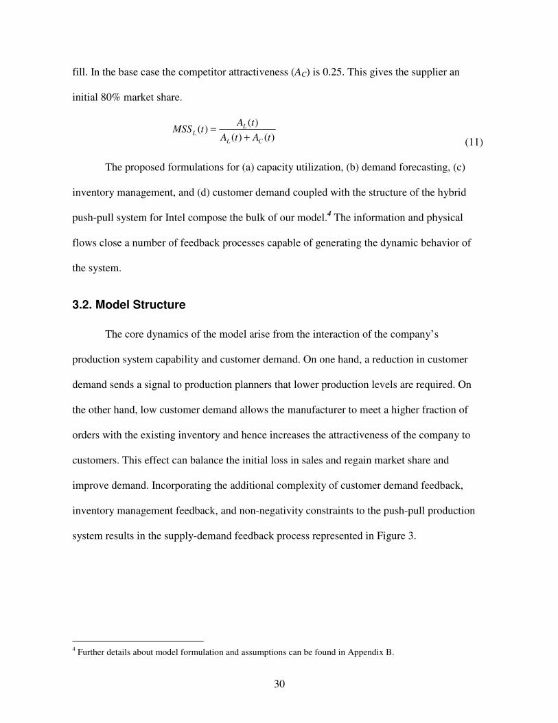
30

fill. In the base case the competitor attractiveness (AC) is 0.25. This gives the supplier an

initial 80% market share.

)()()(

)(tAtA

tAtMSS

CL

LL +

= (11)

The proposed formulations for (a) capacity utilization, (b) demand forecasting, (c)

inventory management, and (d) customer demand coupled with the structure of the hybrid

push-pull system for Intel compose the bulk of our model.4 The information and physical

flows close a number of feedback processes capable of generating the dynamic behavior of

the system.

3.2. Model Structure

The core dynamics of the model arise from the interaction of the company’ s

production system capability and customer demand. On one hand, a reduction in customer

demand sends a signal to production planners that lower production levels are required. On

the other hand, low customer demand allows the manufacturer to meet a higher fraction of

orders with the existing inventory and hence increases the attractiveness of the company to

customers. This effect can balance the initial loss in sales and regain market share and

improve demand. Incorporating the additional complexity of customer demand feedback,

inventory management feedback, and non-negativity constraints to the push-pull production

system results in the supply-demand feedback process represented in Figure 3.

4 Further details about model formulation and assumptions can be found in Appendix B.

31

FabricationWIP

FinishedGoods


GrossProduction

RateShipments

DesiredWaferStarts

MfgCycleTime

-

+ AssemblyWIP Gross

AssemblyCompletion

AWIP*

AWIPAdjust

AWIPAdjustTime

++

-

MarketShare

+

CustomerDemand

+

Fraction ofOrders Filled

-

+


+

+

+

+

-

R1

Growth ThroughService

B5

Lostsales

ForecastedCustomerDemand

B2

AdjustAWIP

+ DELAY

R2

+

ProductionPush

B4 DemandPull

+

DELAY

FabWIP*

FabWIPAdjust

FabWIPAdjustTime

+

-

+

-B1

AdjustFabWIP

FGI*

FGIAdjust

FGIAdjustTime

+

--

+

B3

AdjustFGI

AvailableCapacity

+

Figure 3 – Supply-demand feedback process for a hybrid system.

The following paragraphs describe the individual feedback loops. The first set of loops

– Adjust FabWIP (B1), Adjust AWIP (B2), and Adjust FGI (B3) – describes the inventory

adjustment policies. Managers compare the actual level of inventory with a desired level and

adjust any discrepancy over an adjustment period. In practice, an initial reduction in the

inventory level will cause an increase in the discrepancy to the desired inventory level. This

leads to an increase in production to raise the inventory level and close the inventory gap.

Hence, a change in inventory level creates a feedback process that balances its original effect.

The next balancing loop – Demand Pull (B4) – describes the company’ s replenishment

process as required by the pull system. An increase in shipments decreases the inventory of

finished goods and sends a signal to assemble more chips to replenish finish goods inventory.

Here, a decrease (increase) in finished goods creates a feedback process that balances finished

goods inventory to its desired level. The last balancing loop – Lost Sales (B5) – describes the

company’ s ability to retain customers according to its service level, measured in terms of the

fraction of orders delivered to customers. If the company cannot adequately fill customer

32

orders, it will lose market share to competitors. In practice, an increase in demand will make it

hard to meet all orders. Filling only a fraction of orders leads to unsatisfied customers, lost

sales, and ultimately lower demand. Hence, an increase (decrease) in demand creates a

feedback process that balances its original effect.

The second reinforcing loop – Production Push (R2) – describes the feedback from the

company’ s supply chain to customer demand. This loop captures not only the long delays

associated with customer reactions but also the production delays associated with the

fabrication process. The more (less) microprocessors the company produces and stores in

inventory, the more (less) capable it is of meeting customer demand, the more (less) attractive

it becomes to customers, and the more (less) market share it gains, further increasing

(decreasing) demand.

These feedback processes are capable of generating the dynamic behavior observed in

the company and replicated in the model. The next section explores the dynamic behavior for

different shocks in demand.

4. Model Analysis and Results

The model constitutes a ninth-order system of nonlinear differential equations. Since

the system of equations is highly nonlinear it is not possible obtain closed-form solutions.

Hence, we use simulation to gain intuition about model behavior. Figure 4 shows the behavior

of backlogs and finished goods inventory for two scenarios. In the first scenario, the model

runs in equilibrium with constant demand, and the manufacturing system operates in the

desired way. Figure 4a suggests that under equilibrium the supplier’ s backlog remains

constant and low (1 Million units), allowing it to deliver products to OEMs within the target

delivery delay, or maintaining backlog coverage, of one week (0.25 months). In this scenario,

33

the supplier maintains a constant coverage for finished inventory of one week (Figure 4b) and

fills all (100%) of its customer orders (Figure 5a). Hence, the hybrid push-pull system allows

the company to operate in a highly desirable way.

Backlog Coverage (months)0.50

0.35

0.200 12 24 36 48

Time (Month)

Equilibrium

Pulse 20%

Backlog Coverage (months)0.50

0.35

0.200 12 24 36 48

Time (Month)

Equilibrium

Pulse 20%0.30

0.25

0.200 12 24 36 48

Time (Month)

Finished Inventory Coverage (months)

Equilibrium

Pulse 20%0.30

0.25

0.200 12 24 36 48

Time (Month)

Finished Inventory Coverage (months)

Equilibrium

Pulse 20%

Figure 4 – Backlog and finished inventory coverage for equilibrium and 20% scenarios.

In the second scenario, the base case run for the simulation, we introduce a transient

(single month) 20% increase in customer demand at the end of the first simulated year. Table

1 shows the parameters chosen for the base case. When demand suddenly increases by 20%,

the number of orders backlogged increases, almost doubling the backlog coverage (Figure

4a). Since the supplier cannot raise shipments instantaneously, it is not surprising that backlog

increases. Higher backlogs push the desired shipment rate up (not shown) but since finished

goods inventory (FGI) are not available to support a higher shipment rate, the supplier service

level, the fraction of orders filled (FoF), decreases (Figure 5a).

Table 1. Base Case Parameters

Parameter Definition Value D Customer demand 5 Million units/month

MS Initial market segment share 75% K Available capacity 25,990 wafers/month

DPW Number of die per wafer 200 die/wafer YL Number of good wafers per total produced 90% YD Number of good die per wafer 90% YU Number of good microprocessor units per good die 95%

34

A lower fraction of orders filled can result in customers receiving only a fraction of

what they ordered, or only a fraction of customers receiving their full orders. Customers

respond to the low service level with a delay, accounting for reporting delays in information

systems at OEMs and the supplier and decision making delays (Figure 5b).

Fraction of Orders Filled1.0

0.5

0

Equilibrium

Pulse 20%

0 12 24 36 48Time (Month)

Fraction of Orders Filled1.0

0.5

0

Equilibrium

Pulse 20%

0 12 24 36 48Time (Month)

0 12 24 36 48Time (Month)

Perceived Fraction of Orders Filled1

0.8

0.6

Equilibrium

Pulse 20%

0 12 24 36 48Time (Month)

Perceived Fraction of Orders Filled1

0.8

0.6

Equilibrium

Pulse 20%

Figure 5 – Actual and perceived fraction orders filled for equilibrium and 20%

scenarios.

Consider the information available to managers at the supplier: rising demand,

increasing backlogs, and decreasing service levels. They realize quickly the need to raise

production, i.e. increase the desired wafer starts (Figure 6a). Managers know, however, that

they cannot bring new capacity online in the short-term. Therefore, they raise capacity

utilization (Figure 8b) to increase the number of wafer starts produced (Figure 6b).

Normalized Desired Wafer Starts300

200

100

00 12 24 36 48

Time (Month)

Equilibrium

Pulse 20%

Normalized Desired Wafer Starts300

200

100

00 12 24 36 48

Time (Month)

Equilibrium

Pulse 20%

Normalized Wafer Starts150

100

50

00 12 24 36 48

Time (Month)

Equilibrium

Pulse 20%

Normalized Wafer Starts150

100

50

00 12 24 36 48

Time (Month)

Equilibrium

Pulse 20%

Figure 6 – Desired and actual wafer starts for equilibrium and 20% scenarios.

35

While the desired wafer starts shoot up, the additional production capability available

through higher utilization is limited. Fab managers quickly adjust utilization to the maximum.

The increase in utilization raises the level of fabrication and assembly WIP coverage (Figure

7). As production increases, after a fabrication and assembly delay so does finished goods

inventory (FGI). Total production, however, will take a while before coming online and may

be insufficient to meet all customer orders backlogged. If customers perceive a sustained low

service level, they will turn to competitors. Ultimately, the company’ s inability to meet

customer demand results in a reduced market segment share, offsetting the original increase in

demand (Figure 8a).

Fabrication WIP Coverage (months)

Equilibrium

Pulse 20%

3.75

3.25

2.750 12 24 36 48

Time (Month)

Fabrication WIP Coverage (months)

Equilibrium

Pulse 20%

3.75

3.25

2.750 12 24 36 48

Time (Month)

Assembly WIP Coverage (months)1.2

1.0

0.80 12 24 36 48

Time (Month)

Equilibrium

Pulse 20%

Assembly WIP Coverage (months)1.2

1.0

0.80 12 24 36 48

Time (Month)

Equilibrium

Pulse 20%

Figure 7 – Fabrication and assembly WIP for equilibrium and 20% scenarios.

However, as customer demand decreases, it will eventually equal the volume of

supplier shipments. When orders and shipments equalize, backlogs and the backlog coverage

(Figure 4a) stop increasing and the fraction of orders filled (Figure 5a) stops declining. Since

it takes time for customers to perceive that the company is capable of filling their orders,

market share continues to decrease. Capacity utilization (Figure 8b) drops reflecting the

supplier’ s awareness of decreasing demand. The decrease in utilization lowers the level of

fabrication and assembly WIP coverage (Figure 7). When customers finally perceive

improved company performance, they resume ordering and market share again increases.

36

Over time, orders increase past shipments and again backlogs increase. With a new surge in

orders, shipments may not be sufficient to meet all customers, hence, the fraction of orders

filled decreases. This oscillation decays as the excess demand is lost and the supplier closes

the demand gap with production above normal utilization. Over time, the supplier

performance reaches equilibrium.

Market Share (%)85

80

75

Equilibrium

Pulse 20%

0 12 24 36 48Time (Month)

Market Share (%)85

80

75

Equilibrium

Pulse 20%

0 12 24 36 48Time (Month)

Capacity Utilization1.2

0.8

0.4

0

EquilibriumPulse 20%

0 12 24 36 48Time (Month)

Capacity Utilization1.2

0.8

0.4

0

EquilibriumPulse 20%

0 12 24 36 48Time (Month)

Figure 8 – Capacity Utilization and Market Share for equilibrium and 20% scenarios.

Hence, a transient and moderate (20%) increase in demand decreases the supplier’ s

initial service level and introduces instability to the system, when the company operates with

fixed capacity. As a result of the interaction between customers lost sales loop (B5) and the

company’ s production push (R2) market share as well as fabrication and assembly WIP,

utilization, backlog, finished goods inventory at the supplier oscillate.

The simulation analysis provides some insight into the model behavior, but how is the

behavior sensitive to the assumptions embedded in the nonlinear functions of customer

response and capacity utilization? This question is addressed in the next section, where we

perform sensitivity analysis with respect to such functions.

4.1. Sensitivity Analysis

Model behavior is highly sensitive to the assumptions embedded in the capacity

37

utilization and customer response nonlinear functions. As mentioned earlier, model behavior

is sensitive to the assumptions of (1) the slope of the nonlinear function (f1) of capacity

utilization around the normal operating point and (2) the maximum capacity utilization

possible. In addition, model behavior is sensitive to the customer response assumptions

around (3) the slope of the nonlinear function (f2) and (4) its minimum value. The sensitivity

analysis follows a common procedure to obtain its results. We represent each nonlinear

function (capacity utilization (f1) and customer response (f2)) as a linear combination of two

polar cases, capturing extreme assumptions. By varying the weight in the linear combination

it is possible to obtain a range of behavior in the model.

4.1.1. Sensitivity to Capacity Utilization

Consider the two extreme cases of factory (Fab) managers’ reactions to desired

production: responsive and unresponsive managers. Both managers respond to increases in

desired production volume in the same way, adjusting capacity utilization upwards (to the

maximum utilization level) and increasing total production beyond the normal operating

point. They respond differently though to decreases in the desired production volume. An

unresponsive manager, characterized by function ( f1A), does not respond much to a reduction

in desired production. Despite the low desired production rate, an unresponsive manager will

prefer to keep the machines running and build up inventory levels down the chain, instead of

slowing down production rate. For sufficiently low desired production volumes, however, this

manager would reduce capacity utilization levels. In the extreme case of no desired

production, this manager would not produce anything. The reaction of an unresponsive

manager suggests a flat slope for the capacity utilization function, when desired production is

lower than normal. In contrast, a responsive manager, characterized by function ( f1B),

38

responds aggressively to decreases in desired production. A responsive manager will react to

a decrease in the desired production rate, by slowing down the production rate and allocating

the available capacity for process improvement runs or preventive maintenance. This manager

will avoid building up inventories that may not be used later. Hence, a responsive manager

decreases the capacity utilization rapidly to match the low desired production volume. The

reaction of a responsive manager suggests that the slope for capacity utilization adjustment is

the steepest possible, when the desired production is lower than normal. A general capacity

utilization curve is obtained from the linear combination of the two polar cases (f1A and f1B).5

1B11A1 )1( fwfwCU −+= ; w1∈ [0,1] (12)

Figure 9 shows the results of sensitivity of market share for several specifications of

capacity utilization. The results suggest that system variability increases moderately with

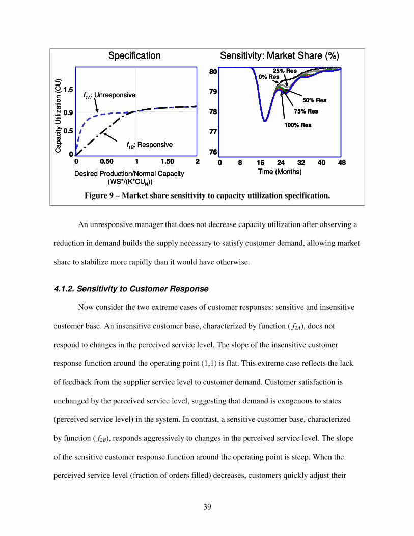
managers’ responsiveness to changes in desired production levels. This result is counter-

intuitive. It was plausible to believe that the supplier would prefer a more responsive

manager, capable of rapidly shifting capacity to other uses and avoiding inventory build-ups

during periods of limited demand. However, inventory build-up is desired since it is the

supplier inability to meet customer demand that causes the reduction in market share.

5 The base case simulation uses w1 = 0.5.

39

Specification

Desired Production/Normal Capacity (WS*/(K*CUN))

f1A: Unresponsive1.5

0.9

0.5

00 0.50 1 1.50 2

f1B: Responsive

Cap

acity

Util

izat

ion

(CU

)Sensitivity: Market Share (%)

Time (Months)

100% Res

75% Res

50% Res

0% Res25% Res80

79

78

77

760 8 16 24 32 40 48

Specification



0.9

0.5

00 0.50 1 1.50 2

f1B: Responsive

Cap

acity

Util

izat

ion

(CU

)Specification



0.9

0.5

00 0.50 1 1.50 2

f1B: Responsive

Cap

acity

Util

izat

ion

(CU

)Sensitivity: Market Share (%)

Time (Months)

100% Res

75% Res

50% Res

0% Res25% Res80

79

78

77

760 8 16 24 32 40 48

Sensitivity: Market Share (%)

Time (Months)

100% Res

75% Res

50% Res

0% Res25% Res80

79

78

77

760 8 16 24 32 40 48

80

79

78

77

760 8 16 24 32 40 48

Figure 9 – Market share sensitivity to capacity utilization specification.

An unresponsive manager that does not decrease capacity utilization after observing a

reduction in demand builds the supply necessary to satisfy customer demand, allowing market

share to stabilize more rapidly than it would have otherwise.

4.1.2. Sensitivity to Customer Response

Now consider the two extreme cases of customer responses: sensitive and insensitive

customer base. An insensitive customer base, characterized by function ( f2A), does not

respond to changes in the perceived service level. The slope of the insensitive customer

response function around the operating point (1,1) is flat. This extreme case reflects the lack

of feedback from the supplier service level to customer demand. Customer satisfaction is

unchanged by the perceived service level, suggesting that demand is exogenous to states

(perceived service level) in the system. In contrast, a sensitive customer base, characterized

by function ( f2B), responds aggressively to changes in the perceived service level. The slope

of the sensitive customer response function around the operating point is steep. When the

perceived service level (fraction of orders filled) decreases, customers quickly adjust their

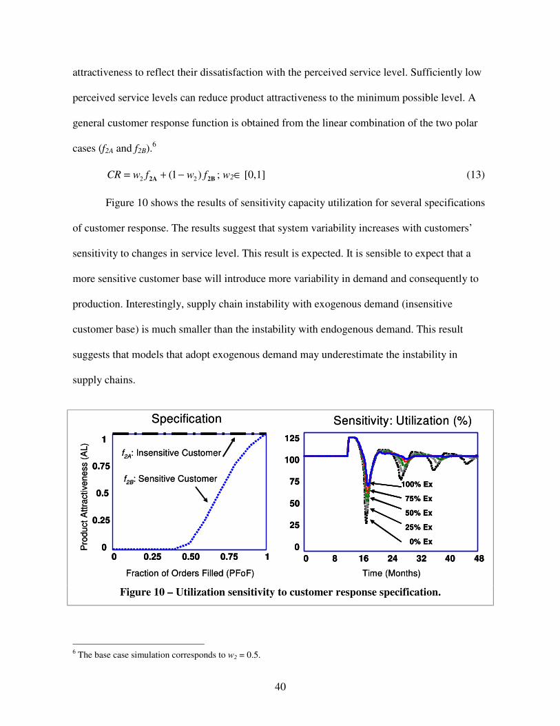
40

attractiveness to reflect their dissatisfaction with the perceived service level. Sufficiently low

perceived service levels can reduce product attractiveness to the minimum possible level. A

general customer response function is obtained from the linear combination of the two polar

cases (f2A and f2B).6

2B2A fwfwCR )1( 22 −+= ; w2∈ [0,1] (13)

Figure 10 shows the results of sensitivity capacity utilization for several specifications

of customer response. The results suggest that system variability increases with customers’

sensitivity to changes in service level. This result is expected. It is sensible to expect that a

more sensitive customer base will introduce more variability in demand and consequently to

production. Interestingly, supply chain instability with exogenous demand (insensitive

customer base) is much smaller than the instability with endogenous demand. This result

suggests that models that adopt exogenous demand may underestimate the instability in

supply chains.

Specification

Fraction of Orders Filled (PFoF)

f2A: Insensitive Customer

f2B: Sensitive Customer

1

0.75

0.5

0.25

00 0.25 0.50 0.75 1

Pro

duct

Attr

activ

enes

s (A

L)

Specification

Fraction of Orders Filled (PFoF)

f2A: Insensitive Customer

f2B: Sensitive Customer

1

0.75

0.5

0.25

00 0.25 0.50 0.75 1

1

0.75

0.5

0.25

00 0.25 0.50 0.75 1

Pro

duct

Attr

activ

enes

s (A

L)

Sensitivity: Utilization (%)

Time (Months)

125

100

75

50

25

00 8 16 24 32 40 48

100% Ex

75% Ex

50% Ex

25% Ex

0% Ex

Sensitivity: Utilization (%)

Time (Months)

125

100

75

50

25

00 8 16 24 32 40 48

100% Ex

75% Ex

50% Ex

25% Ex

0% Ex

125

100

75

50

25

00 8 16 24 32 40 48

100% Ex

75% Ex

50% Ex

25% Ex

0% Ex

Figure 10 – Utilization sensitivity to customer response specification.

6 The base case simulation corresponds to w2 = 0.5.

41

The next section provides a more detailed understanding of model behavior through

eigenvalue analysis. First, it reviews the application of linear systems theory to explore the

dynamics of nonlinear systems. It obtains the modes of behavior for the system. Then,

through eigenvalue evolution plots it investigates the major conditions driving the system into

oscillation.

4.2. Modes of behavior

There are no closed-form solutions for a high-order system of nonlinear ordinary

differential equations (ODEs). Simulation provides many insights into system behavior (as

seen in the previous section). From linear system theory, however, we know that eigenvalues

and eigenvectors characterize all possible modes of behavior in linear ODE systems. Hence,

by linearizing our nonlinear system of equations we can obtain further insights into the modes

of system behavior. Unfortunately, linearized solutions are only a good approximation of

nonlinear systems solutions close to the operating point. Therefore, additional insights

obtained locally through linearization cannot be generalized to the rest of the system. Here,

we circumvent these shortcomings by linearizing the system at every point in time – in

practice, every time step in the simulation – and computing its eigenvalues. In this way, we

obtain specific modes of behavior for different time steps of the simulation. We complement

our understanding of system behavior, extending our local inferences to global

generalizations, through careful analysis of the evolution of the eigenvalues over time.

Finally, we investigate how system behavior changes as a function of the system structure.

We explore how different modes of behavior (eigenvalues) change with different links, and

ultimately, different loops, through link gain elasticity and loop gain elasticity. The

eigenvalue elasticity with respect to a link or a loop provides a deeper understanding of how

42

system structure (links and loops) affects model behavior.7 After linearizing the system at

every point in time, it is possible to express it as

bAxx +=∂∂

t

where A is the state transition matrix, b is the vector of inputs, and x is the state vector. In

particular, the state vector (x) for our ninth order system can be obtained directly by

inspection of equations (B44) – (B52), in appendix B:8

=

=

3

2

1

3

2

1

Filled Orders Fract Perceived

Filled Orders Fract Perceived

Filled Orders Fract PerceivedShipments Expected

Demand ExpectedlogBack

Inventory Goods Finished

WIP Assembly

WIP nFabricatio

PFoF

PFoF

PFoFES

EDB

FGI

AWIP

FabWIP

.

.

.

x

Using the software package AnalyzitTM (Hines 2001), it is possible to obtain the

linearized values for the state transition matrix and its associated eigenvalues. Since our

system is non-linear, the resulting state transition matrix and eigenvalues change over time. In

addition, since the model is capable of generating oscillatory behavior, we expect to obtain at

least one pair of complex eigenvalues in our analytical results. This is confirmed in the

following eigenvalue results for a specific time in the simulation (t = 18 months):

λ1,2 = −0.57 ± 0.86j, λ3,4,5 = -0.5; λ6,7 = −1, λ8,9 = −4

7 More information about the analytical methodology used can be found in Forrester (1982, 1983), Kampmann (1996), and Gonçalves et al. (2000). 8 Note that the perceived fraction of orders filled (PFoF) in the state vector accounts for the three state variables in the third-order Erland delay.

43

Each eigenvalue is associated with a time constant (τ) determined by the real part, and

a period of oscillation (T) determined by the imaginary part according to:

jT

bjaπ

τλ 21 +=±=

We can obtain the time constant (τ) and the period of oscillation (T) for the

eigenvalues obtained earlier (t = 18 months):

jj3.7

275.11

86.057.02,1πλ ±−=±−=

][ 3.7 and ],[ 8.1 2,12,1 MonthsTMonths ==τ

25.05,4,3 −=−=λ ][ 25,4,3 Months=τ

11

17,6−=−=λ ][ 17,6 Months=τ

25.01

49,8−=−=λ ][ 25.09,8 Months=τ

First, we observe that all real eigenvalues have negative values, indicating that the

system is locally stable. More importantly, the only complex pair of eigenvalues indicates that

the oscillatory behavior has a period of oscillation of 7.3 months and a moderate decay time

(1.8 months). This period of oscillation is somewhat smaller than the period of 10 months

observed in the simulation of the full nonlinear system. The eigenvalues above describe the

model behavior at a single point in time. Considering the evolution of the eigenvalues over

time it is possible to understand the system behavior throughout the simulation. In addition,

since model behavior shows damped oscillation (Figure 4-8), it is possible to select a cycle of

the simulation to exemplify the evolution of the eigenvalues.

44

First Complex Eigenvalue Pair

-1

0

1

18 22 26 30 34Time (Months)

Real E1 & E2Imag E2

Imag E1

First Complex Eigenvalue Pair

-1

0

1

18 22 26 30 34Time (Months)

Real E1 & E2Imag E2

Imag E1

Second Complex Eigenvalue Pair

-3

-2

-1

0

1

18 22 26 30 34Time (Months)

Real E3 & E4

Imag E4

Imag E3

Second Complex Eigenvalue Pair

-3

-2

-1

0

1

18 22 26 30 34Time (Months)

Real E3 & E4

Imag E4

Imag E3

Third Complex Eigenvalue Pair

-5

-3

-1

1

18 22 26 30 34Time (Months)

Real E6

Real E5 Imag E6

Imag E5

Third Complex Eigenvalue Pair

-5

-3

-1

1

18 22 26 30 34Time (Months)

Real E6

Real E5 Imag E6

Imag E5

Three Real Eigenvalues

Time (Months)

Real E9

-10

-5

0

18 22 26 30 34

Real E7

Real E8

Three Real Eigenvalues

Time (Months)

Real E9

-10

-5

0

18 22 26 30 34

Real E7

Real E8

Figure 11 – The evolution of eigenvalues in the time domain.

Figure 11 shows the evolution of all nine eigenvalues over the duration of two cycles.

The first cycle (starting shortly after the pulse increase in demand) is representative of the

behavior of other cycles. The evolution plot shows that within the first cycle, the eigenvalues

go through three discrete jumps, indicating three distinct phases of model behavior. Focusing

on the first pair of eigenvalues, we observe that: the eigenvalues become real at t = 17; they

become complex again at t = 19; at t = 21 the real part increases and the complex part

decreases; and at t = 27 the eigenvalues become real again, completing the cycle.

Investigating the behavior of all nine eigenvalues, we observe that in the first phase

( 1917 ≤≤ t ), the system has only one pair of complex eigenvalues. In the second phase

( 2119 ≤≤ t ), the system has three pairs of complex eigenvalues. In the last phase

( 2721 ≤≤ t ), the system still maintains three complex pairs of eigenvalues, but there is a

significant change in their real and imaginary values.

45

The discrete jumps indicate that the system encounters strong nonlinearities that cause

significant changes in the eigenvalues. Between discrete jumps, the eigenvalues remain

almost constant suggesting that the model is roughly piecewise-linear. In a procedure

analogous to the one conducted in phase 1, it is possible to map the eigenvalues for phases 2

and 3. Table 2 provides a summary of the complex eigenvalues (as they provide clues for the

oscillatory behavior observed) and describes the characteristics of system behavior.

Table 2 – Modes of behavior for a non-linear system after eigenvalue evolution analysis

Eigenvalues W��(Months)

Periodicity

(Months) Behavior

Phase1

j86.057.02,1 ±−=λ

8.12,1 =τ 3.72,1 =T One oscillatory mode: • Decaying w/7 mo. period

Phase 2

j6.034.02,1 ±−=λ

j34.11.04,3 ±−=λ j34.068.06,5 ±−=λ

9.22,1 =τ

104,3 =τ

5.16,5 =τ

5.102,1 =T

7.44,3 =T

5.18 6,5 =T

Three oscillatory modes: • Decaying w/11 mo. period

& moderate decay • Decaying w/5 mo. period &

slow decay • Decaying w/19 mo. period

& decay Phase

3 j46.073.02,1 ±−=λ

j56.0012.04,3 ±=λ

j71.036.26,5 ±−=λ

4.12,1 =τ

834,3 =τ

4.06,5 =τ

7.132,1 =T

2.114,3 =T

8.86,5 =T

Three oscillatory modes: • Decaying w/14 mo. period • Expanding w/11 mo. period

& slow growth • Decaying w/9 mo. period &

fast decay

In phase one, the system operates in stability (real part of the eigenvalues is always

negative) oscillating with a period of about 7 months and a moderate decay time. In phase

two, the system has three modes of operation with oscillatory periods of 5, 11, and 19 months.

The oscillatory mode with shorter period (higher frequency) has a much slower decay than the

other two oscillatory modes. The slow decay suggests that the high frequency oscillatory

mode can dominate the overall behavior of the system, indicating higher instability. In phase

46

three, the system has three modes of operation with oscillatory periods of 9, 11, and 14

months. Two complex pairs of eigenvalues with negative real parts have fast and moderate

decay times, indicating that they might be dominated by the growth behavior of the complex

eigenvalue with positive real part. Moreover, the fact that one pair of complex eigenvalues

has positive real part indicates that the system is locally unstable at that time. Hence, a

transition from phase one to two increases the instability of the system due to a higher

frequency oscillation with slower decay time; and a transition from phase two to three

increases the instability of the system due to a complex pair of eigenvalues with positive real

part.

Since the same pair of eigenvalues (λ3,4) is capable of generating the unstable behavior

of the system in phases two and three, we investigate it in greater detail to understand which

feedback loops generate the behavior. Such knowledge can inform managers where to focus

their attention to generate policies capable of addressing the problem. In particular,

understanding how the feedback structure of the model generates the observed behavior is

essential for creating policies that can directly influence behavior. In order to specify which

loops generate the dynamic behavior it is helpful to use eigenvalue elasticity.

4.3. Eigenvalue Elasticity

Eigenvalue elasticity characterizes how certain loops influence the modes of behavior

in the model through their impact in the eigenvalues. The eigenvalues (λ), describing the

behavior modes in a model, are the solutions of the characteristic polynomial (P(λ)), which is

usually specified in terms of link gains (aij).9

9 Linearization allows every variable (vi) to be expressed as a linear combination of other variables (vj ,where j = 1, 2,…, i,…,n) in the model, such that:

47

P(λ ) = λIn − J = 0 (14)

where J is the Jacobian matrix and In is the identity matrix. Nathan Forrester (1982) suggested

measuring the sensitivity (Skij) of an eigenvalue with respect to a specific link by simply

computing the partial derivative of the eigenvalue with respect to the link gain. This would

allow one to understand how the strength of a link could affect specific modes of behavior.

Skij = ∂λk∂aij

(15)

Additionally, one could normalize the sensitivity measure to isolate the effect of the

change from the sizes (values) of eigenvalues and link gains. This normalization could be

obtained by multiplying the sensitivity by the ratio of the link gain to the eigenvalue. Forrester

defined this measure as the eigenvalue elasticity with respect to link gain (Ekij), or link gain

elasticity.

Ekij =∂λk

∂aij

aij

λk

(16)

Analogously, it is possible to write the characteristic polynomial (P(λ)) in terms of the

loop gains (gn) and find the eigenvalue elasticity with respect to loop gain (Ekn), or loop gain

elasticity.10 The loop gain elasticity measures how a specific eigenvalue changes with respect

to changes in a specific loop gain, allowing us to investigate how specific structures affects

model behavior. Although it is not common, Mason’ s rule (Kampmann 1996) provides a

,vav j

jiji ∑=

where, ,a ij ji vv ∂∂= hence, the link gain (aij) is the partial derivative of variable vi with respect to variable vj.

10 The loop gain (gn) is given by the product of all the link gains (aij) of links forming the loop: ∏∈

=Lnij

n aijg

48

general formula for obtaining the characteristic polynomial in terms of the loop gains

(P(λ,gn)), and thus it can be used to obtain eigenvalues in terms of loop gains.11

Ekn =∂λk

∂gn

gn

λk

(17)

The remainder of this section presents the loop gain elasticity analysis for the complex

eigenvalues in each phase. While several first-order loops, a loop passing through a single

state variable, influence the oscillatory behavior, our focus will be on the impact of higher

order loops, feedback loops passing through two or more state variables, on such behavior.

Such emphasis reflects the fact that while system-wide feedbacks are ubiquitous, they often

go unnoticed by managers in the system. For instance, since Fab managers have complete

control of processes within the Fab, they are very aware of the fabrication WIP adjustment

loop (B1). Hence, they would be able to differentiate the fraction of production starts

dedicated to adjusting the fabrication supply line. In contrast, it is unlikely that factory

managers could distinguish the impact of finished goods inventory adjustment, negative loop

(B3), on production. Our interviews suggest that factory managers lack visibility beyond

11 While using Mason’ s rule is a possible way of obtaining the characteristic polynomial (P(λ)) in terms of the loop gains (gn), it is computationally difficult to implement. Alternatively, Hines et al. (2002) obtain Ekn using the fact that any loop is composed by several distinct links, to write the loop gain elasticity in terms of the link gain elasticity.

k

Ljiij

Lmlmlji

Ljiij

lm

k

Lmlmlji

Ljiij

lm

k

k

n

k

n

n

kkn

n

n nn n

a

aa

aa

ggg

Eλ

λλλλ

λ∏

∑ ∏∑ ∏ ∈

∈

−

≠∈∈

−

≠∈

∂∂=

∂∂=

∂∂= ,

,

1

,,,,

1

,,,

∑∈

∂∂

=nLml k

lm

lm

kkn

aa

E, λ

λ

∑∈

=nLji

kijkn EE,

That is, the loop gain elasticity (Ekn) is just the sum of the link gain elasticities (Ekij) of all the links belonging to the loop. This result allows one to use equation (14) to obtain the eigenvalues in terms of the link gains (λDij); then use equation (16) to compute the link gain elasticities (Ekij); and finally sum up the link gain elasticities of the links belonging to a loop to determine the loop gain elasticities (Ekn).

49

assembly. Lack of visibility of the interactions permeating the system would make it even

more difficult for Fab managers to quantify the impact of capacity utilization decisions on

customer satisfaction and its subsequent impact on future production needs – the positive

production push loop (R2). Managers’ access to local and limited information and use of

heuristics to simplify the complexity of the systems in which they are embedded (Kahneman

and Tversky 1982, Morecroft 1983, 1985, Sterman 1994) often lead to measures that can be

effective locally but fail to address system wide effects. Therefore, understanding the

behavior generated by high-order feedback loops, potentially capturing system wide effects,

has the potential to generate the most insight.

4.3.1. Phase-One Analysis

Table 3 presents detailed information on loop gain elasticities for the complex

eigenvalue generating the oscillatory behavior in phase one. There are only two loops

influencing the complex eigenvalue in phase one: a first-order and a second-order loop. Here,

we will briefly discuss the first-order loop to provide the context for further analysis. The

loops are listed in order of the strength of the elasticity of the real part.

Table 3 – Loop gain elasticities for phase one (t = 18) – eigenval. j86.057.02,1 ±−=λ

Loops

(State Variables)

Elasticity

Real part (a)

Elasticity

imaginary part (b)

FabWIP Self-loop

FabWIP Æ FabWIP

-1 -0.052

Fab-Assembly WIP Adjustment

FabWIP Æ AWIP Æ FabWIP

0 1.052

The FabWIP Æ FabWIP loop has a strong influence on the complex eigenvalue,

especially with respect to the impacting on the real part (i.e. the decaying behavior). The loop

50

is composed of all first-order negative loops around FabWIP, including Fab managers’

adjustment of fabrication WIP (B1), but also the decay from gross production. Increasing the

loop gain, i.e., either decreasing the time to update fabrication WIP adjustment (τFabWIP) or

decreasing the manufacturing cycle time (TPT), will mainly increase the speed of the decay

but also reduce the frequency of the oscillation.12 We also observe that one second-order loop

FabWIP Æ AWIP Æ FabWIP, capturing the Assembly WIP adjustment process (B2),

influences the oscillatory behavior. In particular, the loop is capable of increasing the

frequency (reducing the periodicity) of oscillation if we increase its loop gain, which can be

achieved by decreasing the time to adjust Assembly WIP (τAWIP). In addition, a change in the

loop gain of this second order loop does not seem to influence the speed of decay of the

oscillation. The Assembly WIP Adjustment loop seems to characterize the oscillatory mode of

behavior of the system due to the long delays associated with the fabrication process (3

months) and the adjustment of assembly WIP (1 month). While every stock in the system

oscillates, the cause of oscillation is intrinsic to the Fab production-assembly WIP adjustment

loop (B2).

12 Forrester (1982) describes the mechanisms that link (or loop) gain elasticities affect model behavior. The elasticity of the real part impacts the decay (or growth) behavior; the elasticity of the complex part impacts the oscillatory behavior. A positive (negative) complex part elasticity suggests that an increase in the loop gain leads to an increase (decrease) in the frequency of oscillation. A positive (negative) real part elasticity of a reinforcing loop suggests that an increase in the loop gain leads to an increase (decrease) in exponential growth. A positive (negative) real part elasticity of a balancing loop suggests that an increase in the loop gain leads to a decrease (increase) in exponential decay.

51

4.3.2. Phase-Two Analysis

From our previous analysis, we know that we can focus on the eigenvalue contributing

to the instability. Table 4 presents the information on the loop gain elasticities for the complex

eigenvalue j34.11.04,3 ±−=λ in phase two. 13

The strongest influence on the decay rate comes from the first three high-order loops:

(1)FGIÆESÆFGI, (2) PFoFÆ B Æ PFoF, and (3) PFoFÆ FGIÆ PFoF. The first loop

(FGIÆESÆFGI), supplier assembly-pull from expected shipments, captures the feedback

from the supplier’ s own expectation of shipments to decide the production rate out of

assembly WIP (AONet). The supplier assembly-pull from expected shipments loop has the

strongest impact on the real part of the eigenvalue. In particular, an increase in the loop gain

decreases the decay rate. To effectively dampen the oscillatory behavior (i.e., increase the

decay rate of the eigenvalue) it is possible to decrease that loop gain, easily implemented by

increasing the time to compute expected shipments. The second and third loops also impact

the oscillatory behavior in the same way as the first loop, that is, an increase in the loop gain

increases the frequency of oscillation and decreases the decay rate. The second loop (PFoFÆ

BÆ PFoF), lost sales (B5), captures the feedback from customers’ perception in placing new

orders, particularly the adjustment that takes place due to backlog information. The third loop

(PFoFÆ FGIÆ PFoF), assembly-pull from acceptable backlog-MaxShip, captures the

feedback from customers’ perceptions in setting the acceptable backlog and the required pull

of chips from assembly. The path through finished goods inventory (FGI) indicates the

contribution of maximum shipments (SMAX) in determining the fraction of orders filled (FoF).

13 Table C1 (appendix C) presents further detail on the loop gain elasticities for the three pairs of complex eigenvalues in phase two.

52

Table 4 – Loop gain elasticities for phase two (t=20) – eigenval. j34.11.04,3 ±−=λ

Loops

(State Variables)

Elasticity

Real part (a)

Elasticity

imaginary part (b)

Supplier Assembly-Pull from Expected Shipments

FGIÆESÆFGI

236 0.036

Lost Sales (B5)

PFoFÆ B Æ PFoF

38.0 0.32

Assembly-Pull from Acceptable Backlog-MaxShip

PFoFÆ FGI Æ PFoF

35.0 0.20

Assembly-Pull from Actual Backlog

PFoFÆ FGI Æ B Æ PFoF

-31.4 0.52

Assembly-Pull from Acceptable Backlog-Ship*

PFoFÆ B Æ FGI Æ PFoF

24.0 0.66

Supplier Assembly-Pull from Actual Backlog

FGI Æ B Æ FGI

-17.8 0.66

The strongest influence on the frequency comes from the other three high-order loops:

(1)PFoFÆ B Æ FGI Æ PFoF, (2) PFoFÆFGIÆBÆ PFoF, and (3) FGI Æ B ÆFGI. Like the

assembly-pull from acceptable backlog loop, these loops also set the desired assembly pull

with feedback from customer perception. The first loop (PFoFÆ B Æ FGI Æ PFoF), assembly-

pull from actual backlog, captures the importance of the actual backlog to customers’

response in establishing the desired assembly-pull. The second loop (PFoFÆ FGIÆBÆ PFoF),

is analogous to the assembly-pull from acceptable backlog (PFoFÆ FGIÆ PFoF), however,

the additional path though backlog (B) indicates the contribution of desired shipments (S*) in

determining the fraction of orders filled. The third loop (FGI Æ B ÆFGI), supplier assembly-

pull from actual backlog, captures the internal supplier feedback in setting the actual backlog

and the required pull of chips from assembly.

53

The set of loops that influence the main negative eigenvalue in phase two depends on

the interaction of two state variables: Finished Goods Inventory (FGI) and the Perceived

Fraction of Orders Filled (PFoF). On one hand, they capture the essence of the Demand Pull

characteristic of the supply chain, that is, the loops adjust finished goods inventories (FGI)

pulling goods from assembly WIP (AWIP), through signals originated from customers’

perception of past company performance (PFoF). Furthermore, inventory availability at FGI

plays an important role in the system behavior. The fact that FGI appears in the dominant

loop list suggests that it is critical in determining the actual shipment rate. That only takes

place when the company has insufficient finished goods inventory available to sustain the

desired shipment rate, in which case the maximum shipment rate (SMAX) determines actual

shipments (S). Moreover, the Demand Pull from assembly WIP is the main difference

between the model behavior in phases one and two. The two phases share the same complex

eigenvalue due to oscillatory behavior in Fab production-assembly WIP adjustment loop (B2),

but the first phase operates with sufficient inventory to support the desired shipment rate

whereas the second shipments are limited by available FGI.

4.3.3. Phase-Three Analysis

While there are three oscillatory modes of behavior in this phase, we focus our

analysis on the pair of eigenvalues capable of introducing instability ( j56.0012.04,3 ±=λ ).

The eigenvalues and associated loops contributing to the elasticities are sufficiently different

from the previous phases to suggest there will be other drivers of behavior on this phase.

54

Table 5 presents some information on the loop gain elasticities for the complex eigenvalue in

phase two. 14

Table 5 – Loop gain elasticities for phase two (t=20) – eigenval. j56.0012.04,3 ±=λ

Loop Elasticity

Real part (a)

Elasticity

imaginary part (b)

Production Push Through Actual Backlog

PFoFÆ BÆ FabWIPÆ AWIPÆFGIÆ PFoF

35.7 1.19

Production Push Through Acceptable Backlog

PFoF Æ FabWIPÆ AWIPÆFGIÆ PFoF

33.6 0.85

Production Push Through Expected Demand-Ship*

PFoF Æ EDÆ FabWIPÆ AWIPÆFGIÆ BÆ PFoF

32.7 0.87

Supplier Production Push Through Backlog

FGI Æ B Æ FabWIP Æ AWIPÆ FGI

25.1 0.40

Production Push Through Expected Demand-MaxShip

PFoFÆ EDÆ FabWIPÆ AWIPÆFGIÆ PFoF

24.8 0.77

The eigenvalue analysis suggests that a strong influence to the real and complex eparts

of the eigenvalue comes from a set of loops that pushes production from fabrication

(FabWIP) through assembly (AWIP) all the way into finished goods (FGI), the Production

Push loops (R2). These loops adjust work-in-process in assembly and inventory in finished

goods by pushing fabricated wafers to the downstream supply chain. While most of the

influential loops capture the feedback from customers’ perception to the supplier’ s delivery

reliability, individually some reflect the size of actual backlog, acceptable backlog and

expected demand, to determine the desired level of wafer starts. In terms of the elasticities,

the loop gains in the influential loops suggest that if we increase the loop gain we can raise

the frequency of oscillation and the speed of the growth rate.

14 Table C2 (Appendix C) shows the loop gain elasticity for different complex eigenvalues in phase three.

55

Notably, work-in-process availability at assembly plays an important role in the

system behavior during phase three. The fact that assembly WIP (AWIP) appears in the

dominant loop list suggests that it determines the net outflow out of assembly. The gross

completion of assembled dies depends on the assembly rate that is feasible, that is, the amount

of assembly in work-in-process limits the outflow rate of assembly. The system operates in a

push mode. In addition, the assembly completion rate characterizes the main difference

between the model behavior during phase two and three. The first two phases operate with

sufficient assembly WIP to support the pulling from customer demand whereas in the third

phase the company will push all assembled chips downstream only as they become available.

4.3.4. Summary: Eigenvalue Elasticity Analysis

The system operates as desired during phase one. The semiconductor manufacturer

has sufficient assembly work-in-process and finished goods inventory in its supply chain to

support the operation of the system as a hybrid push-pull system. Once the level of finished

goods inventory falls sufficiently, the company can no longer pull product from FGI and

instead will push them through FGI at the rate that they become available. The shift from

pulling products from FGI at the desired rate to pushing them at the maximum shipment rate

characterizes the transition from phase one to two, where two new complex eigenvalue pairs

arises. This system has one oscillatory mode with a short period of oscillation and long decay

time, leading to an increase in instability. At this time, the internal supply chain fails to

operate as designed; instead it will operate as a push-pull-push system, that is, push through

fabrication, pull from assembly WIP, and push through FGI. Phase three characterizes the

shift from assembly-pull to assembly-push. At that time, reduced levels of assembly WIP

cause the supplier to push assembly as they become available from fabrication. When the

56

supplier runs out of assembly WIP the system ceases to operate as a pull; the operation of the

process transitions from a push-pull-push to a pure push system (e.g., a push-pull-push

system). Table 6 provides an overview of the results obtained through the eigenvalue

elasticity analysis, detailing the dominant feedback loops, the active supply chain, binding

constraints, and the impact on behavior.

Table 6 – Summary results from eigenvalue elasticity analysis.

Binding Constraints

Active Supply Chain Dominant

Loop

Impact on Behavior

Phase 1

--- PushÆPullÆPull FabWIP FGI

+

AWIPFabWIP FGI

+

AWIP

Adjust AWIP

(B2)

• Reactive to maintain supply line ( JDLQ IUHTXHQF\�

Phase 2

FGI PushÆPullÆPush FabWIP FGI

+

AWIP

+

FabWIP FGI

+

AWIP

+

Lost Sales (B5)

Demand Pull (B4)

• Increase time to compute Ex. Ships. ( JDLQ IUHTXHQF\

JDLQ �GHFD\�

Phase 3

FGI

AWIP

PushÆPushÆPush FabWIP FGI

+

AWIP

++

FabWIP FGI

+

AWIP

++

Production Push (R2)

• Decrease utilization responsiveness ( JDLQ IUHTXHQF\ JDLQ �JURZWK�

The combination of the information on dominant loops and the impact on behavior

provides a guideline for policy design. Specific policies arise through the reflection of how

certain loop gains impact the decay/growth (real part) and frequency (complex part) of the

eigenvalues. In phase one, managers want to be reactive to changes in assembly work-in-

process to maintain an adequate supply line, which allows the system to maintain sufficient

stock of assembly WIP to meet customer demand. In phase two, managers want to reduce the

customer responsiveness – a loyal and insensitive customer base is preferred – but since this is

difficult to accomplish instead the semiconductor manufacturer can focus on extending the

57

time constant used to compute the expected shipments.15 In phase three, the supplier wants to

decrease the aggressiveness of its adjustment of capacity utilization in response to customer

demand. Here, trying to meet customer demand, while helpful in the short run, may actually

hurt customer service in the long run. By reducing the slope of the nonlinear function (f1) the

supplier can insulate production from oscillations in customer demand originated by poor

service level. The reduction of the slope reduces the gain of the positive Production Push (R2)

loop, locally reducing the frequency and growth of the oscillatory behavior.

The analysis suggests that the hybrid push-pull system is stabilizing only if it can

operate as designed. Low inventory and work-in-process levels, however, may make this a

very hard task to accomplish. Maintaining a stable system may be particularly challenging as

managers in the semiconductor industry constantly face pressures to reduce inventory levels

and meet rapidly changing demand signals. Our analysis suggests that supply chain operation

shifts over time from a desirable push-pull mode, which is stable, to an undesirable pure push

mode, which is unstable. A shift in supplier performance, from high to low, accompanies the

shift in the operation mode. Eigenvalue analysis provides insight on how specific structures

(feedback loops) impact the model behavior at different times, particularly through the

understanding of binding constraints, and dominant feedback structures. Information on

eigenvalue elasticity’ s impact on gain and frequency of oscillation is used in the next section

to derive a policy capable of stabilizing the behavior of the system even under demand

shocks.

15 The result of a loyal customer base is similar to the one provided in the sensitivity analysis: reducing customer responsiveness reduces the slope of the nonlinear function (f2) and reduces the strength of the feedback from service level to market share.

58

4.4. Policy discussion

The eigenvalue analysis suggests that the shift in the mode of operation from a

stabilizing push-pull system to an unstable push system occurs due to stock-outs in upstream

inventories. This result suggests that a policy of maintaining higher upstream inventories

could potentially keep the system within the desired operation mode. There are many

possibilities for designing stabilizing policies for this system. One possibility is to use the

insights about the impact of feedback structures on model behavior to derive policies that can

reduce the stability. Another possibility is to assign costs to important parameters (e.g. service

levels, assembly WIP, finished goods inventory, and market share) and for a set of suggested

inventory policies investigate the coefficients that maximize profits. Alternatively, it is

possible to use the understanding from the eigenvalue elasticity analysis about the drivers of

system behavior to introduce balancing feedback loops that can stabilize the system, or to

break loops that can destabilize the system. While we have performed some simulation

experiments on the possibilities mentioned above, we focus on the first method.

The major policy investigated maintains inventory buffers at AWIP and FGI. The

policy explores a 10% and 20% inventory buffer in AWIP, a 10% and 20% inventory buffer

in FGI and 10% buffer on each AWIP and FGI. Figure 12 shows the results for the policies

implemented. Policies introducing inventory buffers at Assembly WIP are particularly

stabilizing.

59

Market Share

AWIP10%+FGI10%

FGI20%

FGI10%

AWIP20%

AWIP10%

Base

0.81

0.80

0.79

0.780 12 24 36 48

Time (Month)

Market Share

AWIP10%+FGI10%

FGI20%

FGI10%

AWIP20%

AWIP10%

Base

0.81

0.80

0.79

0.780 12 24 36 48

Time (Month) Figure 12 – Stabilizing stock policy at Assembly WIP

A 10% inventory buffer policy at AWIP has a stronger impact on market share than a

20% inventory buffer at FGI. In addition, a 20% inventory buffer policy at AWIP has a

stronger impact on market share than a 10% inventory buffer at AWIP and FGI. The system

faces a reduction of 25% in loss of market share when it carries 10% safety inventory in FGI;

a 46% reduction when it carries 20% of safety stock in FGI; a 55% reduction when it carries

10% of safety stock in AWIP; a 70% improvement when it carries 10% safety stocks in FGI

and AWIP; and a 77% reduction when it carries 20% safety stock in AWIP. Maintaining

safety stock in assembly work-in-process makes the system more robust to shocks in demand

and it is less costly to implement than keeping inventory in finished goods. The safety stock

policy does not prevent the system from entering into a push mode of operation, but it allows

the system to recover in the following cycle.

5. Discussion and Directions for Future Research

This paper addressed the causes of oscillatory behavior in capacity utilization at a

semiconductor manufacturer and the role of endogenous customer demand in influencing the

60

company’ s production and service level. The modeling effort was based on extensive

structured and semi-structured interviews with managers at Intel. The resulting model

constitutes a ninth-order system of nonlinear differential equations, capturing the heuristics

used by managers to run the company. The model runs in continuous time for four simulated

years. The paper contributes to our understanding of the role that customer response has on

increasing demand amplification across supply chains by exploring the mechanisms through

which endogenous customer demand interacts with managers production heuristics. The

results suggest that models assuming exogenous demand may underestimate the impacts of

demand variability. In addition, while hybrid push-pull systems outperform pure pull and

push systems, the analysis suggests that this can only take place if the system actually

operates as designed. Stockouts in different stages in the supply chain can alter the operation

mode of the chain from a desired push-pull system to a pure push system, leading to lower

system performance and instability. The simple heuristics of keeping inventory buffers at

AWIP for improving system robustness, when customers respond to the company’ s variable

service level, should be of great managerial interest. The policy sheds light into the

importance of inventory buffers despite the managerial pressure to against them. The policy

also suggests that the supplier can effectively reduce supply chain instability and reduce the

impact on lost sales and market share.

In general, semiconductor manufacturers, as well as firms in other industries, tend to

keep low inventory levels and run lean supply chains, allowing them to reduce inventory

costs. This practice presents manufacturers with a strategy to avoid costs associated with

inventory obsolescence in industries with short product life cycles. Low inventory and work-

in-process levels, however, may lead to stockouts in different stages in the supply chain,

61

increasing the likelihood that the system will operate in an undesirable mode (e.g., as a push

system). Considering the typical inventory management heuristics adopted by companies, like

the constant adjustment of desired inventory levels to reflect current demand signals, and the

potential increase in demand variability introduced by customer responses, we note that

companies may underestimate the true costs associated with stockouts. Moreover, the research

suggests that managers’ heuristics of adjusting capacity utilization to respond to variability in

demand – caused by the supplier’ s inability to satisfy customer – can amplify the demand

variability. The supplier’ s effort to meet customer demand in the short run may actually hurt

customer service in the long run. Managers must consider the costs associated with decreased

performance, lost sales, and an unstable production system and compare them with the

additional holding costs and potential write-off costs associated with higher inventory levels.

In terms of its theoretical contributions, this research adopts a novel approach to

model analysis that complements simulation of a system of nonlinear ordinary differential

equations. More precisely, this study extends the application of linear systems theory

techniques to analyze nonlinear systems, through eigenvalue evolution plots. Eigenvalue

analysis makes it possible to clarify our understanding of model dynamics. In particular, we

observed that three distinct oscillatory loops dominate the behavior of the system at different

phases. By tracking the evolution of eigenvalues in the time domain, it was possible to

observe that large shifts in the eigenvalues occurred when nonlinear constraints in the system

bind. As the system hit such constraints, the active system changed from a hybrid push-pull

system to a pure push system. The analysis allowed us to understand which parts of the

system were active and contributed to model behavior. In addition, eigenvalue elasticity

provides helpful information for understanding model behavior and designing effective

62

stabilizing policies. Eigenvalue elasticity analysis complements overall understanding of the

system by providing specific information about how certain feedback loops contribute to

model behavior. The next paragraph summarizes the insights provided by the eigenvalue

analysis.

In phase one, the system operates as desired, i.e., as a push-pull-push system. To

maintain an adequate supply line in the chain, managers want to be reactive to changes in

assembly WIP. In phase two, the level of FGI falls sufficiently to prevent the supplier to pull

products from FGI, causing the chain to operate as a push-pull-push system. To prevent the

instability in phase two, managers at the semiconductor manufacturer can increase the time

constant used to compute the expected shipments. In phase three, reduced levels of assembly

WIP cause the supplier to operate as a pure push (e.g., a push-push-push) system. To prevent

the instability in phase three, the supplier wants to decrease the responsiveness of its

utilization adjustment. By trying to be responsive to customer demand in the short run the

supplier may be hurting customer service in the long run.

There are a number of opportunities for future research motivated by this study.

Currently, our study abstracts away from the introduction of new products over time and the

characteristic demand patterns during product introductions. It is possible to incorporate a

demand function that more closely captures the demand experienced by semiconductor

manufacturers during the introduction of new products to investigate the supply chain

behavior under such conditions. In addition, our model incorporates only the response of

customers due to current service level (e.g. supply reliability). However, it is possible that

long-term effects also play an important role in influencing demand. In that sense, if

customers have consistently experienced poor supply reliability, they may choose not to order

63

from that supplier. Another possibility is to explore the application to other industries.

Whereas the semiconductor industry has been characterized by an exponential increase in

demand, many other industries (e.g. automobiles) face almost flat demand. In such industries,

the effects reported here may also play an important role. In terms of supply chains, one

possibility would be to investigate chains with different designs and explore whether the

mode of operation of such chains change over time. Further research on this area could

potentially contribute to improved supply chain designs. Future research could also focus on

exploring the costs and benefits associated with inventory buffers and supply chain instability.

For a set of suggested inventory policies and costs associated with important supply chain

metrics (e.g., service level, assembly WIP, finished goods inventory, and market share), it

would be possible to obtain optimal coefficients to the suggested policies capable of

maximizing profits.

Currently, the model captures only the possibility of lost sales due to product

shortages, that is, that customers seek alternative sources of supply. The current specification

assumes that OEMs do not cancel previous orders after learning about the supplier

unreliability. Cancellations, as well as lost sales, are likely to take place. Incorporating order

cancellations is likely to amplify the effects caused by lost sales, intensifying the OEM

response to a decrease in service levels. Therefore, order cancellations would strengthen the

results presented here. In addition, the current model does not incorporate the possible

inflation of orders by customers, creating phantom demand or bubbles, when multiple OEMs

hedge against supply shortages. While not incorporated in the model, phantom demand is

important since it is likely to balance the effects of lost sales and counter the effects observed

in this research. While not reported here, we incorporated the assumption and conducted a

64

number of simulations to investigate the impact on the results. Our analysis concludes that for

plausible values of inflationary ordering the main results of this paper still hold. While this

study does not incorporate these important assumptions – order cancellation and order

inflation – they have been addressed thoroughly by the author in two other studies (Gonçalves

2002a, 2002b). The hope is that by separating the effects we can help clarify their distinction

and impacts to supply chains.

There is also ample possibility for further research on the methodological front. A

larger body of research using eigenvalue elasticity analysis could provide more insight into its

utility as well as opportunities for improvement. Notably, the technique seems to be

particularly helpful in very complex models, where simulation alone may not be sufficient for

understanding model behavior. In terms of time of analysis, the development of the analysis

on this paper was cumbersome and time consuming. The software can be substantially

improved to generate the eigenvalue evolution plots in the time domain and in the state space.

Here, the development of more intuitive and user-friendly software can bridge this gap and

enable a more wide spread use of the technique.

Finally, the eigenvalue evolution graphs in this research showed sharp transitions from

real to complex eigenvalues. Such transitions provided us clues about binding constraints,

shifts in strong system nonlinearities, and loop dominance; they also indicated focus areas to

further explore the eigenvalue elasticities with respect to loop gains. The sharp transitions are

directly correlated with our use of strong nonlinearities (such as minimum and maximum

functions to characterize the assembly outflow and shipment rates.) We suspect that smoother

functions may generate smoother eigenvalues transitions. It would be interesting to explore

the behavior of systems with different types of nonlinearities to test the applicability of the

65

technique under different model assumptions. From an analytical point of view, however, this

may offer an opportunity for improved model understanding. Researchers can use highly

nonlinear functions at first to gain insight on the overall model and better understanding of the

active system before transitioning to more realistic constraints in a refined model.

7. References

Anderson, E. and C. Fine. 1999. “ Business Cycles and Productivity in Capital Equipment Supply Chains.” In Tayur et al. Quantitative Models for Supply Chain Management. Kluwer Academic Publishers, Norwell, MA.

Baganha, M. and M. Cohen. 1998. “ The Stabilizing Effect of Inventory in Supply Chains.” Operations Research. 46: S72-S83.

Boslet, M. 1998. “ Intel Experiences Some Shortages in Pentium II Chips.” Wall Street Journal. August 14, B5.

Cachon, G. 1999. “ Managing Supply Chain Demand Variability with Scheduled Ordering Policies.” Management Science. 45(6): 843-856.

Chen, F. 1999. “ Decentralized Supply Chains Subject to Information Delays.” Management Science. 45(8): 1076-1090.

Chen, F., Z.Drezner, J.Ryan, and D.Simchi-Levi. 2000. “ Quantifying the Bullwhip Effect in a Simple Supply Chain: The Impact of Forecasting, Lead Times, and Information.” Management Science, 46(3): 436-443.

Croson, R. and K. Donohue. 2000. “ Behavioral Causes of the Bullwhip Effect and the Observed Value of Inventory Information.” Wharton School of Business working paper, University of Pennsylvania.

Cyert, R. and J. March. 1963. “ A Behavioral Theory of the Firm.” Prentice Hall, Englewood Cliffs.NJ.

Dana, J. and N. Petruzzi. 2001. “ Note: The Newsvendor Model with Endogenous Demand.” Management Science. 47(11): 1488-1497.

Diehl, E. and J.D. Sterman. 1995. “ Effects of Feedback Complexity on Dynamic Decision Making.” Organizational Behavior and Human Decision Processes. 62(2): 198-215.

Eberlein, R.L., “ Simplification and Understanding of Models.” System Dynamics Review, 1989. 5(1).

Foremski, T. 1999. “ Intel struggles to meet strong demand for chips,” Financial Times (London), November 18, p.42.

Forrester, J.W. 1958. “ Industrial Dynamics – A Major Breakthrough for Decision Makers.” Harvard Business Review. 36(4): 37-66.

Forrester, J.W. 1961. Industrial Dynamics. Cambridge, MA: Productivity Press.

66

Forrester, J.W. 1968. Principles of Systems. Cambridge, MA: Productivity Press.

Forrester, J.W. 1968. “ Market Growth as Influenced by Capital Investment.” Industrial Management Review. 9(2): 83-105.

Forrester, N. 1982. A Dynamic Synthesis of Basic Macroeconomic Policy: Implications for Stabilization Policy Analysis. Ph.D. Thesis, M.I.T.,1982. Cambridge, MA.

Forrester, N. 1983. “ Eigenvalue Analysis of Dominant Feedback Analysis.” Proceeding of the 1983 International System Dynamics Conference, Plenary Session Papers. System Dynamics Society: Albany, NY. 178-202.

Gans, N. 1999a. “ Customer learningand loyalty when quality is uncertain.” WorkingPaper, OPIM Department, The Wharton School, University of Pennsylvania, Philadelphia, PA.

Gans, N. 1999b. “ Customer loyalty and supply strategies for quality competition.” WorkingPaper, OPIM Department, The Wharton School, University of Pennsylvania, Philadelphia, PA.

Gonçalves, P., C. Lertpattarapong and J. Hines. 2000. “ Implementing Formal Model Analysis.” Proceedings of the 2000 International System Dynamics Conference, Parallel Session Papers. Bergen, Norway. System Dynamics Society: Albany, NY.

Gonçalves, P. 2002a. “Why do Shortages Inflate to Huge Bubbles?” WorkingPaper, Sloan School of Management, Massachusetts Institute of Technology, Cambridge, MA.

Gonçalves, P. 2002b. “Investigating the Causes of Seed Returns in the Agribusiness Industry.” WorkingPaper, Sloan School of Management, Massachusetts Institute of Technology, Cambridge, MA.

Gonçalves, P. 2002c. “ Report on Demand Variability: Intel Interviews” Personal communication.

Gupta, S., J. Steckel and A. Banerji. 1998. “ Dynamic Decision Making in marketing Channels: An Experimental Study of Cycle Time, Shared Information and Consumer Demand Patterns.” Stern School of Business working paper, New York University.

Graves, S. 1999. “ A Single-Item Inventory Model for a Non-Stationary Demand Process.” Manufacturing & Service Operations Management. 1: 50-61.

Hachman, M. 1999. “ MPU Supply Tightening.” EBN Online. Jan. 15. http://www.ebnonline.com/showArticle.jhtml?articleID=2902238

Hachman, M. 2000. “ Despite inventory concerns, Intel sets 4Q fiscal records.” EBN Online. Jan. 13. http://www.ebnonline.com/business/opinion/showArticle.jhtml?articleID=2906438

Hall, J. and E. Porteus. 2000. “ Customer Service Competition in Capacitated Systems.” Manufacturing & Service Operations Management. 2 (2): 144–165

Hines, J. 2001. “ Analyzit™: Link Elasticity Software.”

67

Hines, J., C. Lertpattarapong and P. Gonçalves. 2002. “ Software Implementation for Eigenvalue Elasticity Analysis.” WorkingPaper, Sloan School of Management, Massachusetts Institute of Technology, Cambridge, MA.

Hodgson, T. J. and D. W. Wang. 1991. "Optimal Hybrid Push-Pull Control Strategies for a Parallel Multistage System .1." International Journal of Production Research 29(6): 1279-1287.

Hodgson, T. J. and D. W. Wang. 1991. "Optimal Hybrid Push-Pull Control Strategies for a Parallel Multistage System .2." International Journal of Production Research 29(7): 1453-1460.

Huang, M., D. Wang, et al. 1998. “ A simulation and comparative study of the CONWIP, Kanban and MRP production control systems in a cold rolling plant.” Production Planning & Control 9(8): 803-812.

Kaminsky, P. and D. Simchi-Levi. 1998. “ A New Computerized Beer Game: A Tool for Teaching the Value of Integrated Supply Chain Management.” In Supply Chain and Technology Management. H. Lee and S.M. Ng (eds), The Production and Operations Management Society. 216-225.

Kampmann, C.E. 1996. “ Feedback Loop Gains and System Behavior.” In: Richardson GP and Sterman JD (Eds.) Proceeding of the 1996 International System Dynamics Conference Boston. System Dynamics Society: Albany, NY. 260-263.

Kahneman, D. and A. Tversky. 1982. “ The Simulation Heuristic.” In Kahneman, D. et al.. Judgment Under Uncertainty: Heuristics and Biases. Cambridge University Press, Cambridge.

Lee, H., Padmanabhan, V, and Seungjin Whang. 1997a. “ Information Distortion in a Supply Chain: The Bullwhip Effect.” Management Science. 43(4): 546-558.

Lee, H., Padmanabhan, V, and Seungjin Whang. 1997b. “ The Bullwhip Effect in Supply Chains.” Sloan Management review, Spring: 93-102.

Lee, H. and S. Wang. 1999. “ Decentralized Multi-Echelon Supply Chains: Incentives and Information.” Management Science. 45(5): 633-640.

Mass, N. 1975. “ Economic Cycles: An Analysis of Underlying Causes.” Cambridge, Mass. Wright-Allen Press.

Mitchell, T.W. 1924. “ Competitive Illusion as a Cause of Business Cycles.” Quarterly Journal of Economics, 38(4):p. 631-652.

Morecroft, J.D.W. 1980. “ A Systems Perspective on Material Requirements Planning.” Decision Sciences. 14: 1-18.

Morecroft, J.D.W. 1983. “ System Dynamics: Portraying Bounded Rationality.” Omega. 11(2): 131-142.

Morecroft, J.D.W. 1985. “ Rationality in the Analysis of Behavioral Simulation Models.” Management Science. 31(7): 900-916.

68

Richardson, G.P. 1984. “ Loop Polarity, Loop Dominance, and the Concept of Dominant Polarity.” In Proceeding of the 1984 International System Dynamics Conference. Oslo, Norway.

Richardson, G.P. 1986. “ Dominant Structure.” System Dynamics Review, 2(1): 68-75.

Simon, H.A. 1982. “ Models of Bounded Rationality.” The MIT Press. Cambridge. MA.

Singhal, V. and K. Hendricks. 2002. “ How Supply Chain Glitches Torpedo Shareholder Value.” Supply Chain Management Review. January/February. 18-33.

Souza, C. 2000. “ ...as Intel processor shortage pinches OEM earnings.” EBN Online, Jan. 28. http://www.ebnonline.com/showArticle.jhtml?articleID=2906209

Spearman, M. L. and M. A. Zazanis. 1992. “ Push and Pull Production Systems - Issues and Comparisons.” Operations Research 40(3): 521-532.

Spearman, M. 1992. “ Customer Service in Pull Production Systems.” Operations Research 40(5): 948-958.

Sterman, J.D. 1987. “ Testing Behavioral Simulation Models by Direct Experiment.” Management Science. 33: 1572-1592.

Sterman, J.D. 1989a. “ Modeling Managerial Behavior: Misperceptions of Feedback in a Dynamic Decision Making Experiment.” Management Science. 35(3): 321-339.

Sterman, J.D. 1989b. “ Misperceptions of Feedback in Dynamic Decision making.” Organizational Behavior and Human Decision Sciences. 43(3): 301-335.

Sterman, J.D. 1994. “ Learning In and About Complex Systems.” System Dynamics Review, 10(2): 291-330.

Sterman, J., N. Repenning and F. Kofman. 1997. “ Unanticipated Side Effects of Successful Quality Programs: Exploring a Paradox of Organizational Improvement.” Management Science, April, 503-521.

Sterman, J.D. 2000. “ Business Dynamics: Systems Thinking and Modeling for a Complex World.” Chicago, IL, Irwin-McGraw Hill.

Wang, D. W., X. Z. Chen, et al. 1996. “ Experimental push/pull production planning and control system.” Production Planning & Control 7(3): 236-241.

Wang, D. and C. Xu. 1997. “ Hybrid push pull production control strategy simulation and its applications.” Production Planning & Control 8(2): 142-151.

69

Appendix A: Pure Push, Pure Pull, and Hybrid Push-Pull Systems

Production and distribution, on push production systems, are based on long-term

demand forecasts. In contrast, shipments and assembly are managed based on realized

demand, on pull production systems. Finally, a push-pull production system in manufacturing

is a make-to-order system in which the manufacturer produces component inventory based on

long-term forecasts, while assembly and shipments are based on realized demand.

In his investigation of supply chain variability, Forrester (1958, 1961) represented the

supply chain as a sequence of four stocks in which each of the upstream stocks “ pushed” its

contents into the following downstream stock via a decay process. That is,

dsStockStock

StockStockt

n

sn

n

snntn ∫ −+=

−

−

0

,

1

,10,, )(

ττ

where Stockn,s is the nth stock (or the nth inventory) at time s and where τn is a time

constant representing the average residence time of an object in the nth stock or inventory.

The inflow into the nth stock is 1

,1

−

−

n

snStockτ

which depends only on the upstream stock. In

other words, the upstream stock pushes material into the downstream stock. Similarly, Stockn

pushes its outflow, n

snStock

τ, , into Stockn+1. The inflow into the initial inventory, Stock1,

represents a production planning process that takes information about end-customer demand

(i.e. demand on the last stock in chain) and on the inventory position of the final stock.

70

Stock 1+

Stock 2+

Stock 3 +

TimeConstant 1

-Time

Constant 2Time

Constant 3

- -

DesiredProduction Forecast

CustomerDemand

+

+

Figure A1. Stock-and-flow Diagram for a Push System

A system dynamics representation of a pull system would have each stock “ pulling”

contents from the upstream stock via a goal-gap adjustment process. That is,

dsStockDesStock

pOutReStockDesStock

pOutReStockStockt

n

snnsn

n

snnsnntn ∫

+

+++

−+−

−++=

0 1

,11,1

,,0,, )]()[(

ττ

where DesStockn,s is the desired value for the nth stock (or the nth inventory) at time s. The

inflow into the nth stock allows replenishment of the outflow (RepOutn,s) and adjusts for

discrepancies between the nth stock actual inventory position against a desired goal, over a

certain period of time (n

snsn StockDesStock

τ,, −

).

Stock 1 Stock 2 Stock 3

CustomerDemand

+

+

ReplenishOutflow 3

ReplenishOutflow 2

ReplenishOutflow 1

+ +

++

+

Figure A2. Stock-and-flow Diagram for Pull System

71

In other words, the downstream stock pulls material from the upstream stock.

Similarly, Stockn+1 pulls its inflow, )(1

,11,1

+

+++

−+

n

snnsn

StockDesStockpOutRe

τ, from Stockn. The

outflow from the final stock represents the final customer demand.

Production at Intel takes place in a hybrid push-pull production system, combining

aspects of a push system at the upstream stage and a pull system in downstream stages.

Hodgson and Wang (1991a) provided the first study on hybrid push-pull systems, modeling

the system as a Markov Decision Process (MDP) combining Material Requirements Planning

(push) and Just-In-Time (pull) policies as alternatives in the MDP. In a subsequent work

(1991b) the authors extended their investigation to a more general series/parallel multistage

production system. They found that the best performing strategy used a push (MRP) strategy

at upstream stages of production and a pull (JIT) strategy at the downstream stages. Similarly,

Spearman and Zazanis (1992) investigated the behavior of push-pull systems to explain the

apparent superiority of such systems when compared to pure push or pull systems. Their

results suggested that pull systems are easier to control, tend to have less congestion, and

work in process (WIP) is bounded. They suggested a hybrid push-pull control strategy

analogous to Hodgson and Wang’ s that outperformed the pure strategies. Hodgson and

Wang’ s research motivated a number of experimental studies to test the performance of the

hybrid push-pull production control strategies proposed. Wang et al. (1996) achieve better

planning and control with a software alternative to MRP-II; Wang and Xu (1997) obtain

similar results with their simulation software for mass product manufacturing systems; and so

do Huang et al. (1998) when comparing the performance of MRP, Kanban, and CONWIP

(constant work-in-process) systems.

72

Appendix B: A System Dynamics Model of a Semiconductor

Manufacturer

The model structure consists of two major flows: the flow of materials through the

semiconductor company’ s supply chain and the flow of information, managers’ decision

rules, governing such material flow. Materials flow thought the company’ s supply chain from

wafer starts through assembly according to the manufacturing process (described in section

B.1.) Information flows control the flow of materials (e.g. wafer starts, assembly starts,

assembly completion rate, and shipments) through the company’ s supply chain. The model is

run in continuous time and formulated as a system of nonlinear ordinary differential

equations. The model description can be divided in two sub-sectors: (1) production and

inventory control (section B.2) and (2) distribution and logistics (section B.3.)

B.1. Manufacturing Process

Consider a typical semiconductor manufacturer’ s production system. Production in a

fabrication facility (fab) takes 200 mm/300 mm polished disk-shaped silicon substrates,

known as “ wafers,” as inputs and transforms then into ½-inch square integrated circuits,

known as “ chips.” The manufacturing process is commonly divided into the “ front-end,”

including the initial steps of fabrication and sorting, and the “ back-end,” including

assembly/testing and packaging. In the front-end, the polished silicon wafer disks are

transformed, though a complicated process including several steps of photolithography and

etching, into “ fabricated wafers.” Fabricated wafers are composed of hundreds of square dies.

The actual number of dies per wafer range from 100 to 1000, depending on the chip

architecture – whether the chip is “ logic” or “ memory” chip – and its specific design. Each die

is composed of individual devices such as transistors and memory cells. The good fabricated

73

wafers are sent to assembly/test plants, where they are cut into dies where they can be stored

in warehouses – Assembly Die Inventory (ADI) warehouses, collocated with Assembly/Test

plants. In the back-end, the dies are first tested; upon passing the tests, they receive a

protective package and metal connections, resulting in the microprocessors, or packaged die

products, that can be stored in finished goods warehouses.

The front-end is characterized by a push production system, that is, long-term

forecasts, adjusted weekly to accommodate changes in demand, serve as the basis to initiate

production – also known as “ wafer starts.” In contrast to the front-end, the back end is

characterized by a pull production system. Since not all assembled chips may be in tune with

customer demand, manufacturers assemble and test only those chips that are adequate for

market consumption. Orders for specific products pull die from ADI into assembly/testing.

The assembled products can either be shipped directly to customers to meet demand or simply

be used to adjust the finished goods inventory to desired levels. Therefore, semiconductor

manufacturers operate a hybrid push/pull system, starting production based on long-term

forecasts and assembly based on customer demand.

B.2. Production and Inventory Control

This section describes the hybrid push-pull production process of a semiconductor

manufacturer. The description characterizes first the “ front-end” push fabrication process and

then it explores the “ back-end” pull assembly system.

B.2.1. Production Push

The wafer starts rate (WS), given by the product of capacity utilization (CU) and

available capacity (K), determines the production push. Hence, when production managers

74

receive requests to increase Fab output, they can boost wafer starts by either increasing

capacity or capacity utilization. Since it takes a long time to add new capacity, however, in the

short run production managers can only accommodate increases in wafer starts by changing

capacity utilization. For the purpose of this model, we assume that available capacity is fixed

and it is set at a value just above to the desired production start rate. This assumption captures

the manufacturer’ s policy to run the factory as close as possible to maximum capacity and

make the best use of capital investment. In addition, this assumption does not change the

dynamic behavior of the model in a significant way. In fact, all it does is to require a stronger

exogenous shock to drive the system to the observed behavior.

Capacity utilization is a function (f1) desired wafer starts (WS*) and available capacity.

When the desired wafer starts is high relative to available capacity, managers can increase

capacity utilization to meet the desired production. When desired production is equal to

capacity, capacity utilization is equal to 90%, the normal operating point.16 And when desired

production is low relative to capacity, utilization is also low. Moreover, the utilization curve

lies above the 45o reference line, representing managers’ preference to maintaining high

utilization and building inventory relative to shutting down production lines when desired

production is low.

KtCUtWS ⋅= )()( (B1)

))(

()(*

1 KtWS

ftCU = (B2)

1)2(,9.0)1(,0)0(,0,0,0 111111 ===<′′>′≥ ffffff (B3)

16 We assume that the normal operating point for capacity utilization in this company is equal to 90% of maximum capacity.

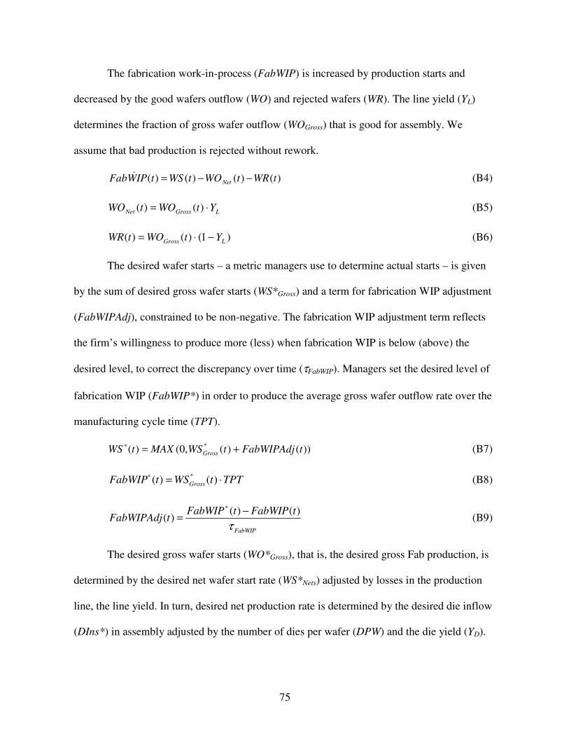
75

The fabrication work-in-process (FabWIP) is increased by production starts and

decreased by the good wafers outflow (WO) and rejected wafers (WR). The line yield (YL)

determines the fraction of gross wafer outflow (WOGross) that is good for assembly. We

assume that bad production is rejected without rework.

)()()()( tWRtWOtWStIPWFab Net −−=� (B4)

LGrossNet YtWOtWO ⋅= )()( (B5)

)1()()( LGross YtWOtWR −⋅= (B6)

The desired wafer starts – a metric managers use to determine actual starts – is given

by the sum of desired gross wafer starts (WS*Gross) and a term for fabrication WIP adjustment

(FabWIPAdj), constrained to be non-negative. The fabrication WIP adjustment term reflects

the firm’ s willingness to produce more (less) when fabrication WIP is below (above) the

desired level, to correct the discrepancy over time (τFabWIP). Managers set the desired level of

fabrication WIP (FabWIP*) in order to produce the average gross wafer outflow rate over the

manufacturing cycle time (TPT).

))()(,0()( * tFabWIPAdjtWSMAXtWS Gross +=∗ (B7)

TPTtWStFabWIP Gross ⋅=∗ )()( * (B8)

FabWIP

tFabWIPtFabWIPtFabWIPAdj

τ)()(

)(−=

∗

(B9)

The desired gross wafer starts (WO*Gross), that is, the desired gross Fab production, is

determined by the desired net wafer start rate (WS*Nets) adjusted by losses in the production

line, the line yield. In turn, desired net production rate is determined by the desired die inflow

(DIns*) in assembly adjusted by the number of dies per wafer (DPW) and the die yield (YD).

76

Where the former variable determines the number of die can be obtained from each wafer and

the latter determines the fraction of good die per wafer.

LNetGross YtWStWS /)()( ** = (B10)

DNet YDPW

tDInstWS

⋅= )(

)(*

* (B11)

Hence, the desired die inflow ultimately drives the desired wafer starts, we note that

this system is pushed by production requests from downstream the Fab. In addition, the sum

of the long-term expected customer demand (ED) and the adjustment from assembly work-in-

process (AWIPAdj) determine the desired die inflow (DIns*).

)/)()(,0()(*UYtEDtAWIPAdjMAXtDIns += (B12)

FabricationWIP

(FabWIP)WaferStarts (WS)

Net WafersOutflow(WOn)

DesiredFabrication

WIP(FabWIP*)

Fabrication WIPAdjustment(FabWIPAdj)

DesiredWafersStarts(WS*)

ManufacturingCycle Time

(TPT)

Time toAdjust

FabricationWIP (Tfw)

-

+

+

-

+

-

+

+

+

InitialFabrication

WIP

WaferRejects

(WR)

+

-+

Desired NetWafer Starts

(WS*n)

+

Line Yield(YL)

-

Desired GrossWafer Starts

(WS*g)+

Gross WafersOutflow (WOg)

AvailableCapacity

(K)

<Desired DieInflow (DIns*)>

Die PerWafer(DPW)

Die PerWafer Yield

(YD)

+

+

--

+

CapacityUtilization

(CU)

Table forCapacityUtilization

(f1)

-

+

Figure B1 – Push system for die fabrication

Figure B1 shows a system dynamics representation of the push production system for

the die fabrication process. Expected demand is simply an exponential smooth of actual

77

orders updated over one year. And the assembly WIP adjustment (AWIPAdj) term reflects the

firm’ s goal to replenish (reduce) assembly WIP when the current level is below (above) the

target to correct the discrepancy over time (τAWIP). The desired level of assembly WIP

(AWIP*) will be explained in the next section.

DAdj

tEDtDtDE

τ)()(

)(−=� (B13)

AWIP

tAWIPtAWIPtAWIPAdj

τ)()(

)(−=

∗

(B14)

B.2.2. Demand Pull

The wafers out of Fabrication are pushed into the Assembly Die Inventory. In

assembly, the wafers are cut into small square dies. Due to the disk-like shape of the wafer

and variability of the fabrication process, only a fraction of the die produced are good enough

to proceed into final assembly. For instance, dies at the margins of the wafer are commonly

scraped. The die per wafer yield (YD) indicates the fraction of good die. So, the product of the

wafers out of fabrication, die per wafer, and die per wafer yield determines the inflow of dies

(DIns) into assembly. While the inflow of dies increase assembly work-in-process (AWIP),

net assembled chip outflow (AONet) and assembly rejects (AR) decrease it. The unit to die

yield (YU) determines the fraction of gross assembled chip outflow (AOGross) that are good and

continue to finished goods inventory (FGI); the remainder, bad assembly, are rejected.

)()( tWOYDPWtDIns NetD ⋅⋅= (B15)

)()()()( tARtAOtDInstIPWA Net −−=� (B16)

UGrossNet YtAOtAO ⋅= )()( (B17)

)1()()( UGross YtAOtAR −⋅= (B18)

78

Gross assembled chip outflow is given by the minimum between the indicated gross

assembled chip outflow rate determined by the production push (PushAOGross) and the desired

gross assembled chip outflow originated by the pull from demand signals (PullAOGross). The

former is given by the feasible completion rate, given by the ratio of available assembly WIP

and the time to complete assembly (τA). The latter is determined by the ratio of the desired

net assembled chip outflow (AO*Net) and the unit to die yield (YU). Hence, when assembly

WIP is sufficiently high assembly is driven by the downstream demand. However, when

inventory is low assembled chip outflow takes place at a rate that is feasible from the

available assembly WIP.

))(),(()( tPullAOtPushAOMINtAO GrossGrossGross = (B19)

AGross tAWIPtPushAO τ)()( = (B20)

UNetGross YtAOtPullAO )()( *= (B21)

Assembled dies increase finished goods inventory and shipments decrease it. The

company will ship as many goods to customers as the desired shipment rate (S*) or as many

as the finish goods inventory can support, that is, the maximum shipment rate (SMax). Hence,

the minimum of the desired and maximum shipment rate determines actual shipments (S). In

addition, the volume of orders in backlog (B) divided by the target delivery delay (DD*)

determines the desired shipments rate. And the maximum shipment rate is given by the ratio

of finished goods of inventory (FGI) and order processing time (τOP).

)()()( tStAOtIGF Net −=� (B22)

))(),(()( * tStSMINtS MAX= (B23)

** )()( DDtBtS = (B24)

79

OPMAX tFGItS τ)()( = (B25)

The desired level of finish goods inventory (FGI*) is given by the product of desired

weeks of inventory (WOI*) and the expected shipments (ES). The latter is simply an

exponential smooth of actual shipments updated over half a week. Managers set weeks of

inventory coverage as the sum of the order processing time (τOP) and the safety stock

coverage (τSS). While inventory coverage may change throughout the life-cycle of a product,

for simplicity we assume a constant coverage policy.17 This assumption is consistent with our

investigation of the production behavior of mature products. Furthermore, by comparing the

desired level of finished goods inventory with the actual level managers can order upstream to

adjust any existing gap in FGI.

)()( ** tESWOItFGI ⋅= (B26)

SAdj

tEStStSE

τ)()(

)(−=� (B27)

SSOPWOI ττ +=* (B28)

FGI

tFGItFGItFGIAdj

τ)()(

)(−=

∗

(B29)

Managers use the information about expected shipments (ES), finished goods

inventory adjustment (FGIAdj), and backlog adjustment (BAdj) to determine the desired net

assembled chip outflow (AO*Net). In addition, managers ensure that the desired net assembled

chips are always non-negative. This request for assembled upstream chips is grossed up into

the desired gross assembled chip outflow (AO*Gross) with the yield for good units (YU) in the

assembly line. 17 For instance, at the early stages of a product life when demand is highly uncertain, inventory managers may adopt a policy of high (e.g. two weeks) inventory coverage. For mature products, with low demand variability, a policy of low (e.g. one week) coverage may suffice.

80

))()()(,0()( tBAdjtFGIAdjtESMAXtAO Net −+=∗ (B30)

UNetGross YtAOtAO )()( ∗∗ = (B31)

FinishedGoods

Inventory(FGI) Shipments (S)

DesiredFinished GoodsInventory (FGI*)

ExpectedSegmentDemand

(ED)

Desired Weeksof Inventory

(WOI*)

FGI Adjustment(FGIAdj)

Desired DieInflow (DIns*)

Time to UpdateOrders (TD)

+

+

-

Time toAdjust FGI

(Tfgi)

+

AssemblyWIP (AWIP)

Net AssemblyOutflow (AOn)

+

Time toComplete

Assembly (TA)

Desired NetAssemblyOutflow(AO*n)

DesiredAssembly WIP

(AWIP*)

AssemblyInventory

Adjustment(AWIPAdj)

Time to AdjustAssembly WIP

(Taw)

+

+

+

-

InitialAssemblyInventory

Die Inflow(DIns)

Die PerWafer(DPW)

Die PerWafer

Yield (YD)

Unit toDie Yield

(YU)

<SegmentDemand (D)>

+

AssemblyRejects

(AR)

GrossAssembly

Outflow (AOg)

++

+-

<BacklogAdjustment

(BAdj)>

+

Desired GrossAssembly Outflow

Pull (PullAOg)+

+

Feasible GrossAssembly OutflowPush (PushAOg)

MaximumShipment Rate

(Smax)

Minimum OrderProcessingTime (Top)

Safety Stock(Tss)

DesiredShipmentRate (S*)

TargetDelivery

Delay (DD*)

<Net WafersOutflow (WOn)>

<Backlog(B)>

-

+

+

+

+ +

-

+

+

+

+

-

+

ExpectedShimpents

(ES)

Time to UpdateShipments (Ts)

<Unit to DieYield (YU)>

Figure B2 – Pull System in the Manufacturing Process

Figure B2 shows the demand-pull system for the assembly/testing process. The

desired level of assembly WIP (AWIP*) is set to produce the average gross assembled outflow

rate over the assembly time (τA). The backlog adjustment (BAdj) term reflects the firm’ s goal

to replenish (reduce) finish goods inventory when the current backlog is above (below) the

target level, to correct the discrepancy over time. The desired level of backlog (B*) is set at a

level that allows the company to meet customer demand within the target delivery delay.

AGrossAOtAWIP τ⋅= ** )( (B32)

FGI

tFGItFGItFGIAdj

τ)()(

)(−=

∗

(B33)

81

B

tBtBtBAdj

τ)()(

)(−=

∗

(B34)

** )()( DDtDtB ⋅= (B35)

B.3. Distribution and Logistics

The manufacturer receives orders from OEMs and other customers. Since orders

cannot be filled immediately, the company keeps a backlog of unfilled orders (B). The

backlog accumulates the discrepancy between customer orders received by the company (D)

and actual shipments (S). If the manufacturer has the finished goods products available in

inventory, it can ship them to customer at the desired shipment rate (S*), otherwise will ship

them as fast as it can (SMax). Overall, the manufacturer’ s ability to fill orders, that is, the

fraction of orders filled (FoF) depends on the ratio between actual (S) and desired shipments

(S*). When actual shipments equal the desired shipment rate, the company is capable of

shipping the full fraction of orders demanded by customers. When actual shipments are lower

than the desired, the company fills only a fraction of its orders.

)()()( tStDtB −=� (B36)

)()()( * tStStFoF = (B37)

Over time, customers respond to the company’ s ability to fill their orders. Future

orders depends on past delivery reliability, that is, the manufacturer’ s past performance in

delivering its products will influence future customer demand. Hence, if the company delivers

a sufficient fraction of its orders, it will fare better than competitors and it will gain market

share. If instead, it cannot adequately fill customer demand, this will erode its market share.

To capture these aspects in the model, we use a third order smooth for the customer

82

perception of fractional orders filled. The six months delay (τF) associated with such smooth

takes into consideration the time customers shape their opinions and purchasing decisions

about products.

3/)()(

)( 11

F

tFoFtPFoFtoFFP

τ−=� (B38)

3/)()(

)( 122

F

tPFoFtPFoFtoFFP

τ−=� (B39)

3/)()(

)( 233

F

tPFoFtPFoFtoFFP

τ−=� (B40)

Furthermore, we assume that delivery reliability is the main feature valued by

customers when modeling the attractiveness of the manufacturer’ s and competitors’ products.

Hence, attractiveness (AL) is a function (f1) of customers’ perceived delivery reliability

(PFoF3). For simplicity, we assume also that competitors maintain a constant delivery

performance, and hence a constant attractiveness level (AC) over time. While this is quite

unlikely, it allows us to measure changes in system behavior directly related to the company

managers’ internal decisions. The manufacturer’ s market segment share is given by the ratio

of the company’ s attractiveness divided by total attractiveness, that is, the sum of the

company’ s and competitor’ s attractiveness. Finally, the product of total demand (TD) for

chips and the company’ s market segment share (MSSL) determines its customer demand (D).

))(()( 32 tPFoFftAL = (B41)

)()()(

)(tAtA

tAtMSS

CL

LL +

= (B42)

)()()( tTDtMSStD L ⋅= (B43)

83

MarketSegment

Share(MSS) Perceived


(PFoF) Time toPerceiveFraction

TotalDemand

(TD)

Table forAttractiveness

(f2)ReferenceFraction of

Orders Filled(FoFR)

CompetitorsAttractiveness

(AC)

TotalAttractiveness

(AT) +- Initial Fraction

of OrdersFilled

Backlog (B)Segment

Demand (D)Order

FulfillmentRate (OF)

AcceptableBacklog

(B*)

BacklogAdjustment

(BAdj)

Time toAdjust

Backlog(TB)

+-

<TargetDelivery

Delay (DD*)>

<Shipments(S)>

DesiredShipment Rate

(S*)<TargetDelivery

Delay (DD*)>

+

+ +

++


(FoF)

ProductAttractiveness (AL)

Figure B3 – Distribution and Logistics

Figure B3 shows the model diagrams for the distribution and logistics sector. Now, we

rewrite the equations to express the system in the following form:

)xf(=x�

where x is the state vector composed by the state variables in our system and x� is its

first derivative with respect to time. The equation suggests that the first derivatives of the state

variables can be written in terms of the vector of state variables. After a long and tedious

algebraic substitution and disregarding the non-negativity constraints, we obtain a system of

nine non-linear differential equations, given by equations (B44) – (B52), in which we will

base our analysis:

84

TPTtFabWIP

KCUK

tFabWIPTPT

YtEDtAWIP

YtB

Y

DDtTDtAtPFoFf

tPFoFf

YtFGI

YtES

CUKYYDPWftIPWFab

FabWIPNFabWIP

AU

AWIP

AUBUB

C

UFGIFGI

SSOP

UNAWIPLD

A

)(}

)()1(

])()()(

)()())((

))((

)()

)(1(

)([{)(

*

32

32

1

−⋅⋅⋅

−+⋅

⋅+−−⋅⋅

+−

−++⋅⋅⋅⋅⋅

=

ττ

ττ

τττ

ττττ

ττ

�

(B44)

))()(

)())(())(()(

)()()(,)(()(

*

32

32

UBUBCUFGI

UFGI

SSOP

UA

LD

YtB

YDDtTD

tAtPFoFftPFoFf

YtFGI

YtES

YtES

tAWIPMINTPT

YFabWIPYDPWtIPWA

τττ

ττττ

−⋅⋅+

−−

⋅++−⋅⋅⋅=�

(B45)

))(,)(())()(

)())(())((

)()()()(,)(()(

*

*

32

32

OPB

C

FGI

SSOPAU

tFGIDDtBMINtBDDtTD

tAtPFoFftPFoFf

tFGItEStESYtAWIPMINtIGF

ττ

ττττ

−−⋅⋅

+−

−⋅++=�

(B46)

))(,)(()()())((

))(()( *

32

32OP

C

tFGIDDtBMINtTDtAtPFoFf

tPFoFftB τ−⋅

+=�

(B47)

DAdj

C

tEDtTDtAtPFoFf

tPFoFf

tDEτ

)()()())((

))((

)( 32

32 −⋅+

=�

(B48)

SAdj

OP tEStFGIDDtBMINtSE

ττ )())(,)((

)(* −

=�

(B49)

))()(3/())(,)((

3/)(

)( *

*1

1 DDtBtFGIDDtBMINtPFoF

toFFPF

OP

F ττ

τ−=�

(B50)

85

3/)()(

)( 122

F

tPFoFtPFoFtoFFP

τ−=�

(B51)

3/)()(

)( 233

F

tPFoFtPFoFtoFFP

τ−=� (B52)

86

Appendix C: Eigenvalue elasticity tables

Table C1 – Loop gain elasticities for phase two (t=20) j6.034.02,1 ±−=λ

Loop Elasticity Real part (a)

Elasticity imaginary part (b)

FabWIP Æ FabWIP -1 -0.052 FabWIP Æ AWIP Æ FabWIP 0 1.052

j34.11.04,3 ±−=λ Loop Elasticity

Real part (a) Elasticity

imaginary part (b) FGIÆESÆFGI 236 0.036

FGIÆFGI -117 -0.25 ESÆES -107 0.19

PFoFÆ B Æ PFoF 38.0 0.32 PFoFÆ FGI Æ PFoF 35.0 0.20

PFoFÆ FGI Æ B Æ PFoF -31.4 0.52 PFoFÆ B Æ FGI Æ PFoF 24.0 0.66

FGI Æ B Æ FGI -17.8 0.66 PFoFÆ PFoF -17.0 -0.017



imaginary part (b) PFoFÆ B Æ PFoF -0.32 0.86

PFoFÆ B Æ FGI Æ PFoF -0.31 0.87 PFoFÆ PFoF -0.22 -0.048

PFoFÆ FGI Æ PFoF -0.20 0.58 PFoFÆ FGI Æ B Æ PFoF -0.17 0.59

FGI Æ B Æ FGI 0.045 0.017 ESÆES 0.045 0.034

FGIÆESÆFGI -0.036 -0.080 FGIÆFGI 0.005 0.028

Table C2 – Loop gain elasticities for phase three (t=21.5)



imaginary part (b) FGI Æ FGI -0.78 -5.86

ESÆ ES -0.75 -7.75

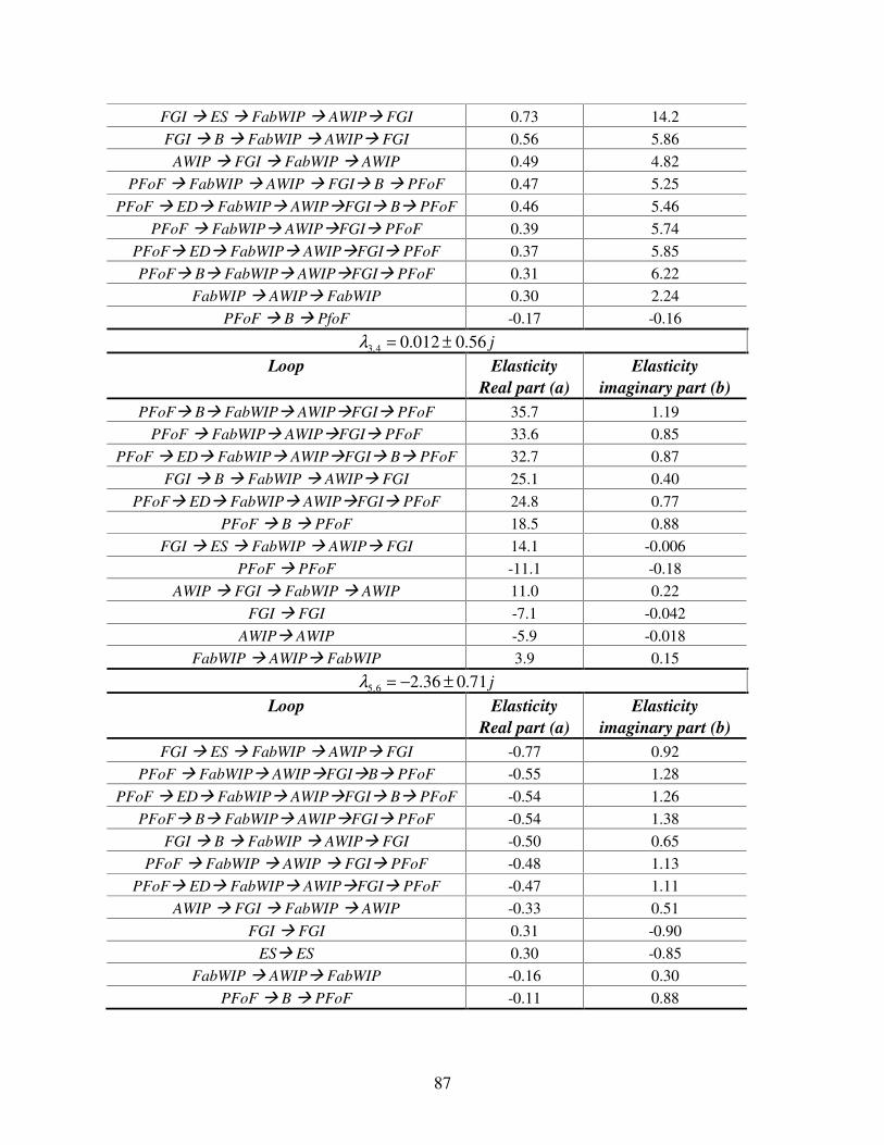
87

FGI Æ ES Æ FabWIP Æ AWIPÆ FGI 0.73 14.2 FGI Æ B Æ FabWIP Æ AWIPÆ FGI 0.56 5.86

AWIP Æ FGI Æ FabWIP Æ AWIP 0.49 4.82 PFoF Æ FabWIP Æ AWIP Æ FGIÆ B Æ PFoF 0.47 5.25

PFoF Æ EDÆ FabWIPÆ AWIPÆFGIÆ BÆ PFoF 0.46 5.46 PFoF Æ FabWIPÆ AWIPÆFGIÆ PFoF 0.39 5.74

PFoFÆ EDÆ FabWIPÆ AWIPÆFGIÆ PFoF 0.37 5.85 PFoFÆ BÆ FabWIPÆ AWIPÆFGIÆ PFoF 0.31 6.22

FabWIP Æ AWIPÆ FabWIP 0.30 2.24 PFoF Æ B Æ PfoF -0.17 -0.16

j56.0012.04,3 ±=λ Loop Elasticity


imaginary part (b) PFoFÆ BÆ FabWIPÆ AWIPÆFGIÆ PFoF 35.7 1.19

PFoF Æ FabWIPÆ AWIPÆFGIÆ PFoF 33.6 0.85 PFoF Æ EDÆ FabWIPÆ AWIPÆFGIÆ BÆ PFoF 32.7 0.87

FGI Æ B Æ FabWIP Æ AWIPÆ FGI 25.1 0.40 PFoFÆ EDÆ FabWIPÆ AWIPÆFGIÆ PFoF 24.8 0.77

PFoF Æ B Æ PFoF 18.5 0.88 FGI Æ ES Æ FabWIP Æ AWIPÆ FGI 14.1 -0.006

PFoF Æ PFoF -11.1 -0.18 AWIP Æ FGI Æ FabWIP Æ AWIP 11.0 0.22

FGI Æ FGI -7.1 -0.042 AWIPÆ AWIP -5.9 -0.018

FabWIP Æ AWIPÆ FabWIP 3.9 0.15 j71.036.26,5 ±−=λ

Loop Elasticity Real part (a)

Elasticity imaginary part (b)

FGI Æ ES Æ FabWIP Æ AWIPÆ FGI -0.77 0.92 PFoF Æ FabWIPÆ AWIPÆFGIÆBÆ PFoF -0.55 1.28

PFoF Æ EDÆ FabWIPÆ AWIPÆFGIÆ BÆ PFoF -0.54 1.26 PFoFÆ BÆ FabWIPÆ AWIPÆFGIÆ PFoF -0.54 1.38

FGI Æ B Æ FabWIP Æ AWIPÆ FGI -0.50 0.65 PFoF Æ FabWIP Æ AWIP Æ FGIÆ PFoF -0.48 1.13

PFoFÆ EDÆ FabWIPÆ AWIPÆFGIÆ PFoF -0.47 1.11 AWIP Æ FGI Æ FabWIP Æ AWIP -0.33 0.51

FGI Æ FGI 0.31 -0.90 ESÆ ES 0.30 -0.85

FabWIP Æ AWIPÆ FabWIP -0.16 0.30 PFoF Æ B Æ PFoF -0.11 0.88

89

Why Do Shortages Inflate To Huge Bubbles?

Paulo Gonçalves



[email protected]

Abstract: When demand exceeds supply, customers often hedge against shortages by placing

multiple orders with multiple suppliers. The resulting demand bubbles creates instability leading to excess capacity, excess inventory, low capacity utilization, and financial and reputation losses for suppliers and customers. This paper contributes to the understanding of demand bubbles caused by shortages by providing a comprehensive causal map of supplier-customer relationships and a formal mathematical model of a subset of those relationships. It provides closed form solutions for supply chain dynamics when supplier capacity is fixed and simulation analysis when it is flexible. Sensitivity analysis provides a deeper understanding of structures and decision rules that contribute to bubbles and suggests policies for improvement. For instance, the ability to quickly build capacity can reduce bubble size. Finally, the time it takes customers to perceive and to react to supply availability is an important lever in controlling demand bubbles. While longer customer perception delays of and slower customer reactions to supply availability stabilizes the entire supply chain, it is harmful to individual customers and it counters conventional wisdom and IT spending on real-time information systems.

Keywords:

System dynamics, supply chain, supply shortages, customer perceptions, order amplification, simulation.

91

1. Motivation

Supply shortages are a recurring supply chain problem, affecting industries ranging

from personal computers to pharmaceuticals. Shortages often take place in industries

characterized by costly capacity and long acquisition delays (Cachon and Lariviere 1999).

They also common accompany the introduction of new products, when demand is uncertain,

and new processes, when production yield is uncertain (Lee et al. 1997a). Shortages often lead

to lower corporate growth (Savage 1999) and loss of shareholder value (Singhal and

Hendricks 2002). In addition, they can lead to excess production capacity and inventories, as

the following example from the semiconductor industry shows (Baljko 1999, Greek 2000).

During a 1995 shortage of microprocessors, suppliers like Intel and AMD had to

allocate production capacity among several customers such as Dell, Compaq, HP, and several

others. To improve their chances of supply, customers placed multiple orders with suppliers.

Since suppliers could not differentiate between final customer demand and direct customer’ s

inflated, “ phantom” orders, suppliers mistook customers’ speculative orders for an increase in

final customer demand. Hence, suppliers responded by increasing stocks of raw materials and

components, speeding up production, adding overtime and building additional production

capacity. However, as production capacity increased, allowing suppliers to meet demand, the

customers’ need to hedge against supply shortages disappeared and so did their speculative

orders. The artificial bubble in demand quickly burst, leaving manufacturers with huge

inventories, excess capacity, and lower prices.

Unfortunately, order cancellations (and product returns) are common in many

industries. Hence, examples of inflated demand generated by product shortages are abundant.

For instance, orders for DRAM chips in the 1980’ s went through a similar process (Li 1992).

92

Hewlett-Packard lost millions of dollars in unnecessary capacity and excess inventory after a

demand surge for its LaserJet printers (Lee et al. 1997b). Facing shortages of Pentium III

processors in November 1999, Intel planned to introduce a new Fab in early 2000 (Foremski

1999). Later that year, blaming order cancellations by large customers and economic

slowdowns, Intel warned that its revenues would fall short of projections and that sales would

be flat for the quarter (Gaither 2001). More recently, Cisco Systems lost over US$ 2.5 billion

in inventory write-offs due to inflated customer orders for their products (Adelman 2001).

While the immediate consequences of shortages are clearly identified in the literature,

some of the long-term impacts and the mechanisms leading to them are not well understood.

This research investigates the impact that agents’ locally rational decisions may have in

reinforcing an initial shortage – or even the rumor of shortage – leading to more dramatic and

long-lasting affects on supply chain performance, and investigates policies for improvement.

The aim is to inform both academics and practitioners dealing with demand bubbles generated

by shortages.18

My analysis suggests that it is locally rational for individual customers to inflate their

orders to get a bigger share of available supply, however, excessive ordering hurts overall

supply chain performance and potentially customers’ own. A temporary shortage in supply

causes high delivery delays and low customer satisfaction. Since it takes time to bring new

capacity online, low supplier performance may lead to customer reactions, such as inflated

orders and ordering from multiple suppliers, generating a bubble in demand. When the

additional capacity becomes available, customers start receiving their orders, and the bubble

created by inflated customer ordering busts. The bust is characterized by a period of order

18 While we describe a hypothetical supplier-customer relationship, demand bubbles can occur at any level in a supply chain.

93

cancellations and depressed customer demand while customers deplete their excess

inventories – an inverse bubble when orders are much lower than they would traditionally be.

As the bubble busts, suppliers are left with excess inventories and capacity greatly exceeding

the amount of product in short supply. Capacity utilization is low, and suppliers and

customers face financial and reputation losses.

The problems associated with demand bubbles are worsened by several aspects such

as customer competition, capacity acquisition delays, and customers’ reaction and perception

delays. First, the size of a bubble is greatly influenced by the amount of competition in the

industry. The fiercer the competition among customers, the stronger the incentive to

customers to respond more aggressively to supply shortages, and the greater the bubble size in

customer’ s orders. To avoid the impact of competition, suppliers may choose to give priority

to preferred customers or to limit the number of customers that they will work with. Second,

the supplier’ s ability to quickly bring capacity online can help reduce the impact of shortage.

A temporary shortage in supply at a supplier with a long capacity acquisition delay –

analogous to fixed capacity – can drive supplier performance out of stability, leading to high

backlogs and delivery delays. Even when capacity acquisition delays are short, the supplier

will face a transient period of low performance, during the delay to bring new capacity online.

In general, the faster the supplier can add new capacity the lower the impacts of the bubble,

that is, it will require less total capacity, it will face a shorter period of low performance

characterized by lower backlogs and shorter delivery delays. While the ability to quickly

bring capacity online helps suppliers reduce bubble size, capacity flexibility alone may not be

a sustainable way to prevent demand bubbles, since it is costly, and suppliers are still left with

some excess capacity.

94

Third, an important leverage point in the system is the time it takes customers to

perceive and react to supplier’ s delivery delays. When a supplier provides real-time

information about delivery delays, customers react instantaneously to the readily available

information, making the system highly unstable. If customers see a high delivery delay they

will respond rapidly and will inflate their orders to hedge against shortages, only making the

situation worst. In contrast, when the supplier provides information about delivery delays with

some delay to customers the system is more stable, because it will take time before customers

over-react, giving the supplier an opportunity to act – speeding up production, increasing

overtime, increasing safety stocks of raw material and components – to reduce delivery

delays. Interestingly, the idea of suppliers providing delayed information about delivery

delays and inventory availability goes in direct opposition to current industry trend to

introduce information systems providing real-time information to all parties in the supply

chain. Unfortunately, these real-time information systems may be introducing a great deal of

instability leading to the creation of larger than ever demand bubbles. While companies claim

to have saved millions of dollars in purchasing and ordering operations through such real-time

systems, the costs associated with over-ordering may far exceed the savings generated from

the accurate processing of orders. A better understanding of the indirect impacts that such

systems can have in inflating these demand bubbles can be very useful to industry

practitioners.

The paper first reviews the relevant academic literature. Section 3 describes the

demand bubble phenomenon and discusses its dynamics. Section 4 presents formal models

followed by results and analyses in section 5. I conclude with implications for theory and

practice.

95

2. Literature Review

There is an extensive system dynamics and operations management literature

addressing inventory instability in supply chains. The first formal system dynamics model on

supply chain instability dates back more than 40 years and coincides with the emergence of

the field of system dynamics (Forrester 1958, 1961). Forrester suggested that fluctuations and

amplifications in supply chains was caused by the structure (including the feedback nature) of

the system. Around 1958, Willard Fey converted this early supply chain work into a game,

which subsequently evolved into the famous beer game. Subsequent system dynamics

research focused on investigating oscillations in different supply chain settings. For instance,

Mass (1975) considered the interrelationship of inventory oscillations and its impacts on a

company’ s labor force. Morecroft (1980) investigated the implementation of Material

Requirements Planning (MRP) systems on a company’ s supply chain and showed that the

faster response time could increase the frequency and amplitude of inventory oscillations.

Motivated by research on bounded rationality and experimental economics,

researchers in system dynamics focused their attention on experimental research. In the

context of supply chains, system dynamicists have focused on characterizing how managers

make decisions and investigating whether such actions can generate pathological dynamics.

For instance, Sterman (1989a, 1989b) conducted human-subject experiments in a four stage

supply chain setting to demonstrate that the sources of oscillation and increase in variability

were managers’ misperceptions of feedback and their inability to account for the supply line

of orders. Diehl and Sterman (1995) continued this work to consider how feedback

complexity in a two-echelon supply chain affected decision-making.

96

In contrast to this behavioral explanation of supply chain instability, the operations

management literature offers a number of operational explanations. For instance, Lee et al.

(1997a, 1997b) suggest that rational agents are able to generate demand variability through

four operational causes: demand signal processing, rationing (supply shortages), order

processing, and price variations. Chen et al. (2000) verify that the bullwhip effect can arise

from two causes: a specific demand forecasting technique and order lead times. While the

dispute among researchers defending operational or behavioral causes of supply chain

instability is far from over, a recent article by Croson and Donohue (2000) suggests that the

bullwhip effect still exists in the absence of three (e.g. price fluctuations, order batching and

demand estimation) out of the four normal operational causes offered by Lee et al. (1997a,

1997b). Their study does not control for product shortages, which is the emphasis of this

paper.

Papers addressing supply shortages emphasize two aspects: the games that take place

among different agents and the impact that the product allocation mechanism has on

customers’ demand variability. For instance, Lee et al. (1997a) develop a single period model

with rational agents to show that strategic behavior among customers, leading to demand

inflation, can take place when the supplier allocates insufficient capacity in proportion to

customer orders. The supplier in their model has imperfect information since she cannot

distinguish final customer demand from those inflated by direct customers. The authors

suggest that capacity allocation in proportion to past sales (turn–and–earn) can mitigate this

problem, but they do not model this case. Cachon and Lariviere (1999a) examine how a turn–

and–earn allocation mechanism impacts customer behavior and supply chain performance,

showing that it allows suppliers to improve profits at the expense of customers’ and even the

97

supply chain’ s performance. Cachon and Lariviere (1999b) explore the impact of other

allocation mechanisms and the supplier’ s decision to build capacity. They build a multi-

period model where suppliers choose the allocation scheme, customers place their orders and

then suppliers decide on how much capacity to build. They find that no truth-inducing

allocation mechanism can maximize customer profits, and attempts to implement such a

mechanism may result in lower profits for all (supplier, customers, and the supply chain).

While previous research on demand variability provides a rich context for the impact

of shortages, the emphasis on game theory requires equilibrium and supply chain assumptions

that may not be realistic in real supply chains. This papers expands on this research by

investigating out-of-equilibrium dynamics and more realistic production physics, such as: (a)

continuous time, instead of stylized single-shot or sequential games, or discrete time models

with often common time delays between all actions; (b) capacity constraints due to long

capacity acquisition delays; (c) endogenous and variable delivery delays, due to changing

order backlog and supplier capacity; and (d) perception and backlog adjustment delays, rather

than instantaneous access to information and immediate adjustment to desired levels. Finally,

whereas previous research has focused on different allocation mechanisms, I propose to

investigate how different parameters (capacity acquisition delays, customer competition,

customers’ reaction and perception delays, etc.) influence the size of demand bubbles under a

proportional allocation mechanism.

98

Orders

Shipments

7�VV,�ji8�AB,

��t|N6jit

$�ijW|��t|N6ji

Orders

Shipments




Orders

Shipments

7�VV,�ji7�VV,�ji7�VV,�ji8�AB,

��t|N6jit

$�ijW|��t|N6ji$�ijW|

��t|N6ji

Orders

Shipments


��t|N6ji


��t|N6ji


��t|N6ji

Figure 1. Supply chain structure

3. Positive Feedbacks in Supply Chains

In a decentralized chain with a single supplier and multiple direct customers (Figure

1), I hypothesize that customers inflate orders when insufficient supply is allocated in

proportion to customer orders. At the time of introduction, the supplier receives initial orders

for the product. Customers adjust their orders until the supply line of orders placed with the

supplier matches the desired order backlog, forming the negative loop (B1), called Adjust the

Supply Line in Figure 2. The supplier bases production on the channel’ s initial orders, but

when a sudden increase in demand occurs, customers face long delivery delays and high

delivery uncertainty. Customers must wait weeks before receiving the partial orders of desired

products. How should customers react to long delivery delays and receipt of partial orders?

Consider customers’ reactions to an increase in delivery delay. Even in the absence of

competition, customers must increase orders to bring the supply line in line with the new

perceived delivery delay. Rational customers adjust the increase in the delivery delay by

ordering ahead of their needs. For instance, if customers keep a supply line of 2 weeks of

inventory to meet expected sales for a product with a 2 week delivery delay, once the supplier

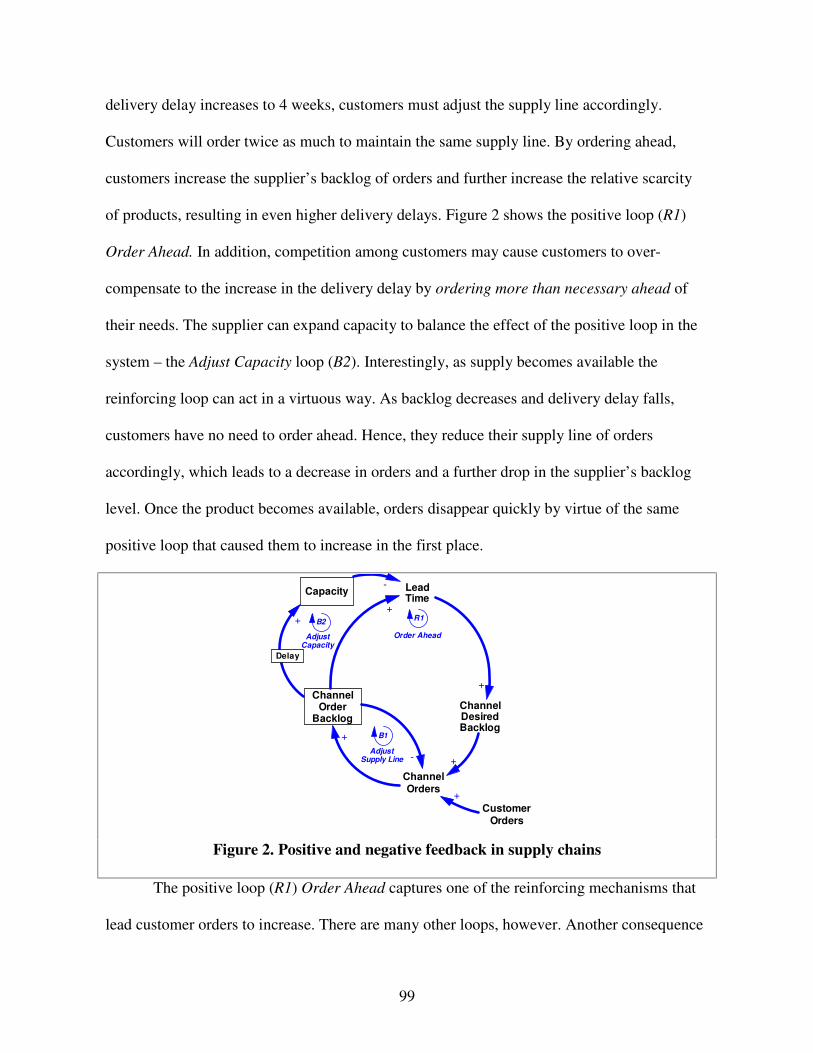
99

delivery delay increases to 4 weeks, customers must adjust the supply line accordingly.

Customers will order twice as much to maintain the same supply line. By ordering ahead,

customers increase the supplier’ s backlog of orders and further increase the relative scarcity

of products, resulting in even higher delivery delays. Figure 2 shows the positive loop (R1)

Order Ahead. In addition, competition among customers may cause customers to over-

compensate to the increase in the delivery delay by ordering more than necessary ahead of

their needs. The supplier can expand capacity to balance the effect of the positive loop in the

system – the Adjust Capacity loop (B2). Interestingly, as supply becomes available the

reinforcing loop can act in a virtuous way. As backlog decreases and delivery delay falls,

customers have no need to order ahead. Hence, they reduce their supply line of orders

accordingly, which leads to a decrease in orders and a further drop in the supplier’ s backlog

level. Once the product becomes available, orders disappear quickly by virtue of the same

positive loop that caused them to increase in the first place.

ChannelOrder

BacklogChannelDesiredBacklog

CustomerOrders

LeadTime

ChannelOrders

+

+

+

+

-

B1

AdjustSupply Line

R1

Order Ahead

Capacity-

+

+

Delay

B2

AdjustCapacity

Figure 2. Positive and negative feedback in supply chains

The positive loop (R1) Order Ahead captures one of the reinforcing mechanisms that

lead customer orders to increase. There are many other loops, however. Another consequence

100

of longer lead times and lower delivery predictability is customers’ desire to build up safety

stocks. However, customers must place more orders to build up safety stocks, which increases

the supplier’ s order backlogs and makes future lead times even longer. Figure 3 shows the

reinforcing loop (R2) Correct Inventory to Lead Time.

Now, consider the customers’ reactions to receiving only a fraction of their orders. As

supplier shipments fall short of customer orders, customers lose trust in the supplier’ s delivery

reliability and adjust to a reduction in supplier reliability by ordering more than necessary. If

customers expect to receive just a fraction of their total orders, they inflate orders – ordering

defensively – in hopes of getting just what they need. For instance, if customers have been

receiving half of their orders when the supplier allocates capacity in proportion to his orders,

they double their orders hoping to get the quantity desired. By ordering defensively customers

increase the supplier’ s backlog of orders even further, resulting in an even more restrictive

allocation policy. Furthermore, customers increase their safety stocks in response to reduced

delivery reliability – correcting inventory to delivery reliability. But to increase their safety

stocks customers must place even higher orders building up supplier’ s backlog of orders even

further. This results in an even tighter allocation policy and a further decrease in delivery

reliability. Figure 3 shows the reinforcing loops (R3) Order Defensively and (R4) Correct

Inventory to Delivery Reliability.

101

ChannelOrder

BacklogChannelDesiredBacklog

CustomerOrders

LeadTime

ChannelOrders

DeliveryReliability

+

+

+

+

-

B1

AdjustSupply Line

R3

OrderDefensively

R1

Order Ahead

Capacity-

DesiredSafetyStock

DesiredInventory

+

+

+

-

+

R2

CorrectInventory toLead Time

R4

CorrectInventory to

DeliveryReliability

+

Delay

B2

AdjustCapacity

-

-

Figure 3. Complete customers’ reactions in supply chains

From the description above, it appears that the characteristic behavior of demand

bubbles would be represented by an overshoot-and-collapse in orders due to customers’

response to a supply shortage. During the initial period of shortage, customers overreact,

inflating the demand bubble through over-ordering. Then, as supply normalizes, the bubble

busts as customers cancel outstanding orders. The reinforcing loops described above make the

system intrinsically unstable, allowing small perturbations and even the rumor of shortages –

similar to self-fulfilling prophecies (Merton, 1948) – to trigger a demand bubble. In industries

where new products introductions are frequent, shortages may occur often due to uncertain

demand for new products, uncertain production yields for new processes, and long capacity

acquisition delays (due to long decision and physical construction delays). Hence, repeated

cycles of sharp overshoot-and-collapse in orders typical of demand bubbles can occur just as

frequently as shortages do. In addition, since these demand bubbles occur during supply

shortages, the bubbles will not take place in a periodic way like typical Bullwhip Effect

oscillations. In that sense, understanding why and when shortages take place can be very

helpful in mitigating their impacts.

102

To gain a deeper understanding of the processes generating demand bubbles and to

investigate policies that can effectively mitigate their impact, next I build a formal

mathematical model of key relationships discussed above.

4. The Model

The model emphasizes the internal causes of system behavior. In particular, the focus

is on customers’ endogenous reactions to supply shortages. The model presented here

includes only one of the possible customers’ reinforcing loops: the Ordering Ahead (R1) loop.

While this provides a limited view of the problem complexity, it is capable of generating the

demand bubble phenomenon. Including other reinforcing loops would only make the problem

more pronounced. For the sake of simplicity, I consider the relationship of a single supplier

selling a single product to multiple customers. The supplier’ s backlog of orders (B) increases

by customer demand (Rd) and decreases by shipments (S) and cancellations (C).

CSRB d −−=� (1)

Customer demand has two terms: a final customer demand (d) and a term for backlog

adjustment. The first term accounts for replenishment orders that direct customers place based

on observed final customer demand.19 The second term is the adjustment between the desired

channel backlog (B*) and suppliers’ actual backlog. This term allows the supplier to adjust her

backlog over an adjustment time (τB) if she observes an increasing desire for her products.

Finally, customer demand must be non-negative.

),0(B

dBB

dMAXRτ−+=

∗

(2)

19 Naturally, final customers may be playing the same game of inflating their orders to direct customers. We assume that direct customers will simply try to meet final customer demand.

103

Consider now the flows of shipments and cancellations. The minimum of desired

shipment rate (S*) and available capacity (K) determine the amount of shipments (S). That is,

shipments will normally be determined by the desired shipment rate unless there is

insufficient capacity. The desired shipment rate depends on the ratio of backlog and the target

delivery delay (τD), as shown in equation 3.

),( KBMINSDτ= (3)

Cancellations depend on the difference between total shipments received by customers

(Sr) and total customer orders (Dc). If there are more shipments received by direct customers

(due to large orders) than final customer orders, then the outstanding excess orders are

cancelled with the time to cancel orders (τC). On the other hand, if customers’ received

shipments are lower than orders there are no cancellations (equation 4).

),0(C

cr DSMAXC τ−= (4)

The supplier’ s capacity (K) is an exponential smooth of customer demand (Rd)

(equation 5), with a time constant given by the time to build capacity ( Kτ ). This formulation

suggests that the supplier tries to keep sufficient capacity to meet customer demand, adjusting

any discrepancies within the time to build capacity.

K

d KRK

τ−=� (5)

Moreover, the amount of total shipments received by customers (Sr) accumulates

supplier’ s shipments to customers (equation 6). Note that while the customers exaggerate their

orders, they only start canceling them once they have received more than they need. Total

customer orders (Dc) simply accumulate true customer demand (equation 7).

104

),( KBMINSD

r τ=� (6)

dDc =� (7)

An additional simplifying assumption allows the supplier to maintain a fixed market

share over time. While prolonged poor reliability will, in general, lead to loss of market share,

suppliers with unique products or other sources of monopoly power can retain market share

despite poor performance. To represent customers, I aggregate them into a single customer.

This assumes homogeneity among different customers, that is, that they will influence model

behavior in the same way due to shortages. This assumption does not hold in general since

customers have different size, negotiating power, inventory policies, and so forth. However,

customers react in a similar way to an increase in delivery delays. When delivery delay is

larger than desired, customers tend to inflate their orders. Evidence supporting this appears

both in practice (Greek 2000) and academia (Lee 1997a). While still a simplifying

assumption, customer homogeneity suffices to address the research purpose, of investigating

how agents’ locally rational decisions may affect supply chain performance by reinforcing an

initial shortage. In particular, the assumption provides insight on the average customer order

inflation and instead of specific order quantities from different customers. Future research

emphasizing customer heterogeneity may inform how competition among individual

customers may further affect supply chain performance. Furthermore, I assume that customers

can cancel orders without incurring any penalties. In many industries (e.g. semiconductors,

networking equipment, electronics, agribusiness, and several others), the supplier adopts

lenient returns policies and “ no penalty” cancellation policies to improve sales.

The desired channel backlog (B*) is a function (f) of delivery delays (DD), which is

given by the ratio of backlog (B) to shipments (S).

105

)(*

SBfdB ⋅= (8)

The function (f) of delivery delay represents customers’ response to supplier’ s ability

to fill demand, that is, it captures customers’ locally rational behavior of placing speculative

orders when the delivery delays increase above normal. In particular, when faced with long

delivery delays customers order ahead, that is, they increase their expected delay above the

delivery delay quoted by the supplier. Increasing their expected delay is intendedly rational to

customers, since they believe that the supplier will try to avoid losing sales at all costs, even

by giving a delivery delay quote that is more optimistic that what it really is. The customer’ s

bias can be captured in a number of different ways. In the simplest case, I assume a

customer’ s bias proportional to the actual delivery delay quoted by the supplier. Hence,

customers’ response to delivery delays can be captured by a linear function of delivery delay

with a slope of α.20 21

xxf ⋅= α)( , where α≥1 (9)

The function (f) embeds the assumption that supplier shipments will be

proportionately distributed among customers. The business press provides ample anecdotal

evidence for customer’ s speculative ordering behavior under proportional allocation (Greek

2000). Academic research also supports this assumption. Using a game theory model, Lee et

al. (1997a) show that customers behave strategically, inflating orders, when a supplier

allocates capacity in proportion to orders. Hence, in aggregate, customers’ action to inflate

orders is intendedly rational. It is rational for customers to place more orders than necessary

20 I also assume that when delivery delays are lower than the target, customers simply adjust their ordering without a bias. 21 A linear function, capturing the proportional bias of customers, is useful to obtain a closed-form solution to the problem, when the supplier has fixed capacity. Closed-form solutions cannot be obtained when the supplier has flexible capacity. In that case, a more general non-linear logistic function (f) can be used to capture strong adjustments for short delivery delays and saturation effects for large delivery delays.

106

because the more they order, under a proportional allocation mechanism, the more products

they are likely to receive. In industries plagued by such customer behavior the costs

associated with over-ordering (penalties for cancellations and returns – if they exist) are much

smaller than the costs associated with under-ordering (unsatisfied customers, unrealized sales

and potential loss in market share). All such aspects provide an additional incentive for

customers’ strategic behavior. Finally, customers will cancel orders once the total number of

products received from suppliers surpasses the total demand from customers as shown in

equation 4.

Now consider the supplier’ s actions. One possibility is to assume that the supplier

does not respond strategically to customers’ order inflation, that is, the supplier is oblivious to

customers’ actions despite order cancellations and product returns. This does not seem

plausible. Alternatively, it is possible to assume that over time the supplier learns to discount

customer orders when delivery delays are high. Consider the outcome. When the supplier

discounts the orders received she intensifies the product rationing perceived by customers,

resulting in even more inflated orders. Again, the supplier knows better than to believe the

customer, so she discounts part of the orders and sends whatever she has (or what she believes

appropriate). The problem is that the supplier does not know true customer demand, making it

difficult for her to assess how much to discount. Consequently, customers will always have an

advantage in their ability to order more to compensate for supplier’ s actions. Even when

suppliers are compensating for customer orders it is plausible to assume that order inflation

will prevail. Instead of explicitly representing the supplier’ s discounting of customers orders,

it is possible to interpret the shape of the function as the net result of customers’ and

supplier’ s actions.

107

In terms of the supplier’ s operations, she adjusts her backlog level according to the

desired channel backlog and she attempts to fill orders to maintain a desired target delivery

delay. Capacity constraints, however, can limit the supplier’ s ability to ship, causing delivery

delays to increase. Finally, the supplier can expand capacity as she perceives demand to

increase. Figure 4 shows the system dynamics model described above.

7�VV,�ji $�ijW|��t|N6jit

8�AB,��t|N6jit

OrderBacklog

(B)

ChannelDesiredBacklog

CustomerOrders

LeadTime

ChannelOrders

CumulativeShipments (Sr)

+

++

+

-

B1

AdjustSupply Line

B3

CancellationsR1

Order Ahead

Capacity(K)

-

ExcessShipments

CumulativeDemand (Dc)

+

+

+

+

+

+Delay

B2

AdjustCapacity

-

-

ChannelDemand (R)

Shipments (S)

Cancellations(C)

7�VV,�ji $�ijW|��t|N6jit

8�AB,��t|N6jit

OrderBacklog

(B)

ChannelDesiredBacklog

CustomerOrders

LeadTime

ChannelOrders

CumulativeShipments (Sr)

+

++

+

-

B1

AdjustSupply Line

B3

CancellationsR1

Order Ahead

Capacity(K)

-

ExcessShipments

CumulativeDemand (Dc)

+

+

+

+

+

+Delay

B2

AdjustCapacity

-

-

ChannelDemand (R)

Shipments (S)

Cancellations(C)

Figure 4. Model diagram for supplier-customer system

The set of differential equations (10-13) below represent the fourth order system of

first order non-linear differential equations associated with the diagram above.

dDc =� (10)

),( KBMINSD

r τ=� (11)

KB

D KBKBMINBfd

dKττ

τ 1]

)),(/([ ⋅−

−⋅+=� (12)

108

),0(),())),(/(

,0(C

cr

DB

D DSMAXKBMINBKBMINBfd

dMAXB ττττ −−−

−⋅+=�

(13)

5. Model Analysis

This section investigates the behavior of the supplier-customer system in greater

detail. First, it provides a closed form solution to the system when the supplier has fixed

capacity. Then, it considers the system behavior when the supplier has flexibility to change

capacity. Since this change increases model complexity significantly, insights in this case are

derived from simulation. Finally, the last section provides sensitivity analysis to explore the

impact of important parameters on model behavior.

5.1. Fixed Supplier Capacity

First, I investigate model behavior when the supplier does not introduce new capacity.

Fixed capacity may result when bringing new capacity online takes several years or it is too

costly to be considered as an option to address shot-term shortages. Fixed capacity can be

implemented by setting the time to build capacity (τK) to an extremely high value, which has

the equivalent effect of breaking the feedback link from supplier demand to available

capacity. I simulate the model for five years, starting from steady state equilibrium. From

equilibrium, I introduce a shock on actual customer demand. The shock, used to investigate

model behavior, is composed of a transient increase followed by a transient decrease in

demand. In particular, the magnitude of the shock is composed of a 10% temporary increase

(a pulse starting at t = 6, lasting for 6 months) followed by a 10% temporary decrease (a pulse

starting at t = 12, lasting for 6 months) in demand (Figure 5). Since the magnitude and

109

duration of the supply shortage is the same as the excess supply, they compensate each other,

that is, average customer demand that year remains at the equilibrium level and equals the

supplier’ s capacity. While the supplier cannot meet all customer demand during the supply

shortage period, it can meet all unsatisfied demand that has been backlogged during the

supply excess period.

<≤<≤⋅−<≤⋅+

=Ttt if K

ttt if K

ttt if K

d0

2

21

1

,,)1(,)1(

ββ

(14)

Actual Demand125

100

750 12 24 36 48 60

Time (Month)

12 Months

Actual Demand125

100

750 12 24 36 48 60

Time (Month)

12 Months

Figure 5. A transient increase and decrease in customer demand

If customers are not responding strategically to the initial shortage, that is if they are

simply adjusting the supply line to account for the increase in delivery delays, the system

should return to equilibrium after the shock in customer demand. Therefore, any change in

model behavior from the equilibrium position captures customers’ responses to relative

shortages in supply. That is, if customers do not over-react during the supply shortage period,

the period of excess capacity is exactly sufficient to bring the system back to equilibrium.

During the high demand period customers do not receive all orders placed. However, during

110

the low demand period suppliers have a chance to meet the excess demand from the previous

period exactly due to the symmetry of the shock.

When the supplier has fixed capacity, it is not able to meet all customer orders;

customers do not have a reason to cancel any orders. If cancellations do not take place, they

do not affect the state of the supplier’ s backlog or customer’ s response. Hence, we can

simplify our system of equations by removing the equations associated with cancellations.

The information necessary to determine the time and volume of cancellations (equation 4)

comes from equations (10) and (11), computing cumulative customer orders (Dc) and

shipments received by customers (Sr), respectively. Removing equations (10) and (11), and

taking away the term for cancellations in equation 13, results in the following simplified

system (15-16).

KB

D KBKBMINBfd

dKττ

τ 1]

)),(/([ ⋅−

−⋅+=� (15)

),())),(/(

,0( KBMINBKBMINBfd

dMAXBDB

D

τττ −

−⋅+=� (16)

where d is given by (14) and the right hand side of the differential equations are written in

terms of the state variables of the system and the shock input.

In addition, equation (15) describes the change in capacity (K) to meet changes in the

supplier’ s backlog position and in customers’ demand. When capacity is fixed the rate of

change in capacity is zero ( 0=K� ), reducing equation (15) to a constant (K). The system with

no cancellations and fixed capacity is reduced to equation (16). Hence, the fourth order

system of nonlinear differential equations (10-13) can be reduced to a first order nonlinear

system. In addition, when capacity is fixed and there is excess customer demand, the supplier

111

cannot ship to customers within the target delivery delay. Instead, shipments are constrained

by available capacity (K). Equation (16) can be further simplified by resolving the

nonlinearity associated with the minimum of the desired shipment rate (D

Bτ ) and the feasible

shipment rate (K). Equation (17) shows the resulting system.

KBKBfd

dBB

−−⋅+=τ

)/(� (17)

Finally, the nonlinear system (17) can be simplified further by considering a linear

function (f = α B/K, where the slope α>1) for customers’ response to delivery delays, which

captures a customers’ bias proportional to the actual delivery delay – the higher the delivery

delay the higher customers’ expected delivery delay.22 The fixed capacity system, with linear

customer response, is given by equation (18).

KBKBd

dBB

−−⋅⋅+=τ

α /� (18)

Now, let B

Kdτ

αγ 1/ −⋅= and let ϕ = d – K. Substituting (14) into (18) yields:

ϕγ =− BB� (19)

where:

<≤−

<≤−−

<≤+−

=

Ttt if

ttt if

ttt if

B

B

0B

2

21

1

,)1(

,)1(

,)1(

τα

ταβα

ταβα

γ

and

<≤<≤⋅−

<≤⋅=−=

Ttt if

ttt if K

ttt if K

Kd0

2

21

1

,0,

,β

βϕ

Note that the equilibrium for the model is given by γϕ−=B and that γ represents the

eigenvalues of the system. Hence, it is possible to describe the system stability for each

22 Under fixed capacity delivery delay never drops below one; hence, there is no need to worry about order deflation.

112

region. Given that α > 1, we note that in the first region ( 1ttt0 <≤ ) the eigenvalue is real and

positive resulting in an unstable system. Since the supplier’ s capacity is smaller than demand,

customers inflate orders and backlog increases exponentially with a growth rate of

Bταβα +− )1( . In region two ( 2ttt1 <≤ ), when demand drops below the supplier capacity, the

system is still unstable if α

αβ 1−< , that is, when the relative aggressiveness of customers’

responses ( αα 1− ) is larger than the percentage increase in demand (β). Hence, very

aggressive customers will continue to increase their orders even when the system has excess

capacity to meet customer demand. Moreover, when customers are not aggressive, the system

is stable and backlogs decrease exponentially to equilibrium with a rate of Bτ

αβα −− )1( .

Note that for α > 1, the rate of growth in period one is strictly higher than the rate of decline

in period two. Hence the supplier backlog cannot return to the initial level after the period of

excess supply. The difference between the initial backlog and the backlog level at the end of

period two captures the impact of customers’ aggressiveness to the supplier. In the last period

( Ttt2 <≤ ), the system is always unstable for α > 1, since the eigenvalue γ is given by

Bτ

α )1( − . Note that when α = 1, that is, when customers order the exact amount to perfectly

compensate for the delivery delay they experience (non-strategic customers), the previous

results change. First, the rate of growth (Bτ

β ) in the first period equals the rate of decline

(Bτ

β− ) in the second period. Hence, backlogs can return to the initial equilibrium level when

the magnitude and duration of excess demand is the same as the excess supply. Finally, when

α = 1, the eigenvalue in the last period ( Ttt2 <≤ ) becomes zero (γ = 0), revealing that the

113

system will remain in equilibrium. It is possible to write the equations for backlog over time,

by finding the solution (equation 20) to the first order differential equation given by equation

(19).

teCtB ⋅⋅+−= γ

γϕ

)( (20)

And, when t0 = 0, eγt =1. So: γϕ+= iBC , where

Ttt ifittt ifittt if i <<=<<=<<= 22110 ,3;,2;,1

i

itt

i

ii

iieBtBγϕ

γϕ γ −⋅+= −⋅ )()()(

<≤⋅

<≤+⋅−−

−

<≤−⋅+−

+

=

−⋅−

−−−⋅−−

+−

−⋅+−

TttifeB

tttifKeK

B

ttifKeK

B

tB

tt

Btt

B

Btt

B

B

B

B

2

)()1(

2

21)1(

)()1(

1

10)1(

)()1(

0

,

,))1(

(

t ,))1(

(

)(

2

1

0

τα

αβατ

αβα

αβατ

αβα

τβαβα

τβ

τβαβα

τβ

(21)

To further describe the behavior of customers, we include a saturation effect for the

maximum delivery delay (M) tolerated by customers. This effect captures customers’ decision

to stop inflating their orders and start looking for alternative sources of supply when the

delivery delay rises to an unacceptable level. A saturation effect takes place at the third stage

when Bτ

αγ 1−= and ϕ = 0. Substituting into (19) and considering that during the saturation

αΒ = ΜΚ, yields:

BB

MKBB

ττ=+�

(22)

MKeMKBB BStt

S +⋅−=−−

τ)(

)( (23)

114

The equation for supplier backlog, when customers tolerate a maximum delivery

delay, is a goal seeking behavior that leads to a final equilibrium value of MK. Now consider

the range of possible customers’ reactions, which can range from the non-strategic to the very

aggressive. A non-strategic customer will adjust his orders exactly to compensate for the

increase in delivery delay. In this case, the slope of the customers’ response to delivery delay

function is one (α = 1). An aggressive customer will adjust orders by much more than the

required compensation. The slope of the expected delivery delay function is more than one (α

>> 1) such that the relative aggressiveness of customers’ responses ( αα 1− ) is higher than the

percentage increase in demand (β). A strategic customer will still adjust orders by more than

the required amount but the relative aggressiveness of customers’ responses is lower than the

percentage increase in demand. As seen in the earlier derivation, even non-strategic customers

will order more during shortages to compensate for the supplier’ s inability to meet demand.

However, as soon as demand falls, customers reduce their ordering accordingly until the

suppliers’ backlog returns to equilibrium. Strategic customers, however, order more than

necessary to compensate for periods of short supply. While the backlog decreases when there

is excess supply, it never falls back to the initial equilibrium level. In addition, since delivery

delays are above normal, customers have a consistent bias to inflate orders, and the supplier

has fixed capacity, the system becomes unstable. Customer orders increase until the delivery

delay is high enough to reach the saturation level, where customers will seek alternative

sources of supply. When saturation is binding, the system reaches a low performance

equilibrium, characterized by extremely high delivery delays and order backlogs. For

instance, the value of the delivery delay equals the saturation delivery delay (M) and the

equilibrium level for the supplier’ s backlog equals the product of customer demand and the

115

saturation delay (KM). In reality, the equilibrium is temporary as customers seek alternative

sources of supply and the supplier invests in new capacity, but the results suggest that lack of

capacity flexibility during supply shortages will lead to system instability if customers behave

strategically. Figure 6 shows the behavior of supplier backlogs, with the introduction of a

saturation effect.

Backlog1,000

750

500

250

00 12 24 36 48 60

Time (Month)

Aggressive

Strategic

Non-Strategic

Backlog1,000

750

500

250

00 12 24 36 48 60

Time (Month)

Aggressive

Strategic

Non-Strategic

Figure 6. Supplier’s backlog with saturation effects23

In summary, when supplier capacity is fixed, it is possible to obtain closed form

solutions for the behavior of the supplier’ s backlog. When customers behave non-strategically

– ordering the exact amount to compensate for changes in the delivery delay – a temporary

supply shortage causes system performance to decrease, leading to higher backlogs and longer

delivery delays. A period of excess supply of same magnitude and duration allows the system

to recover to its equilibrium level. On the other hand, when customers are strategic, a

temporary supply shortage can drive the system out of stability, with escalating order

backlogs and delivery delays. When supplier capacity is fixed and customers order

strategically to compensate for high delivery delays, the reinforcing behavior of the Ordering

Ahead loop (R1) dominates the behavior of the system. Customers continue to place inflated

23 Where the following parameters have been used: β =0.1, Ma = 10, Mn = 7.5, K = 4,000, αa = 1.2, α n = 1.05. And the graph for backlog is normalized to 100.

116

orders (increasing the supplier’ s backlog) until they reach the limiting constraint of their

saturation level. Most suppliers will invest in new capacity once they experience sustained

shortages. The next section investigates the impact of capacity flexibility on system behavior.

5.2. Variable Supplier Capacity

Allowing the supplier to introduce new capacity makes the system much harder to

solve.24 Hence, I simulate the model for five years (from equilibrium) with a transient

increase in demand to gain intuition about model behavior. Then, at the end of the first year, I

allow a transitory 10% increase in demand that lasts one year.

Shipments and Capacity150

100

50

00 12 24 36 48 60

Time (Month)

Demand

Shipments

Capacity

Shipments and Capacity150

100

50

00 12 24 36 48 60

Time (Month)

Demand

Shipments

Capacity

Backlog600

400

200

00 12 24 36 48 60

Time (Month)

Backlog

Steady State

Desired Backlog

Backlog600

400

200

00 12 24 36 48 60

Time (Month)

Backlog600

400

200

00 12 24 36 48 60

Time (Month)

Backlog

Steady State

Desired Backlog

Figure 7. Supplier’s (a) shipments, capacity, and (b) backlog for a 10% transient

increase in customer demand

Figure 7(a) shows demand, shipments and capacity for the supplier; figure 7(b) shows

supplier actual and desired backlog compared to the steady state equilibrium. Due to the

increase in final customer demand, direct customer orders surpass supplier capacity causing

an increase in backlog. Over time, the supplier builds capacity to meet the increase in

demand. At the end of year two, available capacity finally meets customer demand, but

customers still inflate their orders due to large backlogs and delivery delays. Since supplier

capacity is still insufficient to meet customers’ inflated demand, backlogs continue to

24 It results in the fourth-order system (10–13) of nonlinear differential equations presented in section 4.

117

increase. The supplier continues to invest in capacity to satisfy a booming market. The

increase in supplier’ s capacity and backlog represents an important aspect of system behavior.

While customer demand increases by 10% for one year, capacity increases by more than 30%

in reaction to balance the order inflation by customers. Comparatively, backlog increases by

300% relative to its equilibrium level in response to the transient increase in demand.

When supplier shipments finally meet orders, the backlog reaches its maximum. At

the same time, as more capacity becomes available and shipments increase, delivery delay

decreases. Customers respond to lower deliver delays by not inflating their orders. In fact,

customers start canceling orders as supply availability normalizes and total customer orders

increase beyond total customer orders. Interestingly, the initial boom of the demand bubble is

in sharp contrast with the steep decrease in orders that takes place when the bubble bursts.

The burst is characterized by a sharp increase in order cancellations followed by a period of

reduced demand while customers deplete their excess inventories. Figure 8 shows the

evolution of supplier’ s actual and customer’ s expected delivery delays as well as customers’

order cancellations.

Delivery Delay6

4

2

00 12 24 36 48 60

Time (Month)

Actual

Expected

Delivery Delay6

4

2

00 12 24 36 48 60

Time (Month)

Actual

Expected

Cancellations150

100

00 12 24 36 48 60

Time (Month)

Cancellations150

100

00 12 24 36 48 60

Time (Month) Figure 8. (a) Delivery delays and (b) cancellations for a 10% transient increase in

customer demand

The relationship between delivery delays and supply-demand imbalance becomes

clear in the phase plot (Figure 9). As shortages take place and total customer orders (Dc)

118

exceed the total amount of orders received by customers (Sr), the expected delivery delay

increases. Also, since the supply-demand imbalance is given by the difference between total

orders received by direct customers and final customer orders (Sr – Dc), the supply-demand

imbalance becomes negative. As a result of long delays, customers inflate their orders and

over time the supplier invests in new capacity to meet the perceived growth in demand. As

new supplier capacity becomes available, the supplier can increase shipments, preventing the

supply-demand gap from decreasing further. However, delivery delay continues to increase

because supplier backlogs still incorporate customers’ inflated orders. In fact, even when

there is no supply-demand imbalance (Sr – Dc= 0), the supplier still holds high backlogs,

which translate into high delivery delays and further inflated orders.

Phase Plot6

4

2

0-3000 0 3000 6000

Supply Demand Imbalance = Sr – Dc

6

4

2

0-3000 0 3000 6000

Exp

ecte

d D

eliv

ery

Del

ay 6

4

2

0-3000 0 3000 6000

6

4

2

0-3000 0 3000 6000

Phase Plot6

4

2

0-3000 0 3000 6000

Supply Demand Imbalance = Sr – Dc

6

4

2

0-3000 0 3000 6000

Exp

ecte

d D

eliv

ery

Del

ay 6

4

2

0-3000 0 3000 6000

6

4

2

0-3000 0 3000 6000

Figure 9. Phase plot supply-demand imbalance for a 10% transient increase in customer demand

When the supply-demand gap becomes positive, customers start canceling inflated

orders. However, backlogs and delivery delays will continue to increase while customer

demand is larger than the sum of shipments and cancellations. As the supply-demand

imbalance increases, customers cancel a greater fraction of their orders. With more supplier

capacity available, suppliers can ship at a faster rate, run down their backlogs, and decrease

119

delivery delays. Customers adjust to shorter delivery delays by not inflating their orders. The

positive loop that caused customer order inflation begins to act in the opposite direction,

resulting in reduced customer orders. Consequently, the bubble busts, leading customers to

cancel previously placed “ phantom” orders, reducing customer demand. In addition, suppliers

are left with excess capacity and run-down backlogs.

Over time, the additional capacity and the improved performance (low delivery delay)

of the supplier permits backlog to return to the initial equilibrium condition. But as figure 7

shows it takes more than one year after the shortage in supply for backlog to return to

equilibrium. Finally, since capacity acquisition and disposal takes much longer, capacity is

still above the equilibrium level three years after the end of the shortage in supply. To get

further insight into the model the following sections provide sensitivity analysis on several

model parameters.

5.3. Parametric Sensitivity Analysis

This section investigates the sensitivity of the model behavior with respect to changes

in the time it takes the supplier to build capacity, the time it takes customers’ to perceive the

actual delivery delay quote provided by suppliers, and customers’ reactions to delivery delay.

For the first two tests, I run the simulation model allowing the parameter to be twice as high

and half as low as the base case run. For the last test, I introduce different behavioral

functions for customers’ responses. The results suggest that supplier ability to build capacity

quickly can effectively reduce the bubble size. In addition, the time it takes customers to

perceive the supplier’ s delivery delay is an important lever in controlling customers’

inflationary ordering. Finally, customers’ reactions to the delays tend to be more pronounced

in industries where competition among players is intense.

120

5.3.1. Time to build capacity ( Kτ )

First, I test how the model behaves under different capacity acquisition delays ranging

from 4 to 30 months, with an interval of 2 months. Figure 10 shows backlog and capacity.

Shorter capacity acquisition delays lead to lower capacity and backlog levels and earlier

peaks. Longer capacity acquisition delays result in a higher capacity and backlog levels, later

peaks, and a longer period of excess capacity. The results suggest that the supplier’ s ability to

build capacity quickly can reduce the size of the bubble and the duration of the problem.

Since introducing new capacity typically requires long delays, companies have devised

strategies to give them flexibility to ramp up production. In particular, the semiconductor

industry raises the building infrastructure (the shell) well in advance of need such that it does

not become an additional constraint in ramping up production of a new fabrication facility.

The equipment then is positioned as it becomes necessary. While rapidly building capacity

prevents the bubble from growing, it is important to notice that even when capacity can be

quickly introduced, backlogs still doubled in size, for a 10% increase in demand.

012

2436

4860

0

100

200

300

400

500

600

700

800

Time (Months)

Time to Build Capacity (TK)

Backlog

700-800

600-700

500-600

400-500

300-400

200-300

100-200

0-100

10 20 30

012

2436

4860

0

100

200

300

400

500

600

700

800

Time (Months)

Time to Build Capacity (TK)

Backlog

700-800

600-700

500-600

400-500

300-400

200-300

100-200

0-100

700-800

600-700

500-600

400-500

300-400

200-300

100-200

0-100

10 20 30

012

2436

4860

100

110

120

130

140

150

Time (Months)Time to Build Capacity (TK)

Capacity

140-150130-140120-130

110-120

100-110

10 2030

012

2436

4860

100

110

120

130

140

150

Time (Months)Time to Build Capacity (TK)

Capacity

140-150130-140120-130

110-120

100-110

140-150130-140120-130

110-120

100-110

10 2030

Figure 10. Supplier’s (a) backlog and (b) capacity with different delays to build capacity.

Suppliers often have the flexibility of adding capacity to deal with a long trend

increase in demand. But capacity expansion is always costly and once the investment has been

121

made suppliers would like to make the most out of it. However, we observe that due to the

order inflation, suppliers tend to introduce much more capacity – the longer the delay in

introducing capacity the higher the capacity commitments – than the actual increase in

customer demand. Unfortunately, the additional capacity brought online is poorly utilized. As

soon as the bubble collapses, the supplier is left with unutilized excess capacity. Actually, the

situation portrayed in the model is very conservative since it assumes that it is possible to

shed capacity as quickly as it can be acquired. This assumption often does not hold. A more

realistic assumption, accounting for longer delays in reducing production capacity, would lead

to higher excess capacity for suppliers. Hence, while capacity flexibility mitigates the

problem, by itself it may not be an effective means to deal with the impact of customer

strategic ordering due to shortages.

5.3.2. Time for Customers’ to Perceive Delivery Delay

I now examine the model’ s sensitivity to the perception delay customers experience

before they learn about the supplier’ s quoted delivery delay. Nowadays, customers face

virtually no perception delay due to state-of-the-art information systems. Such information

systems allow customers to get real-time information about supply available to promise and

delivery quotes when placing an order. However, this push towards system integration and

information sharing often takes place when there is a dominant player in a supply chain.

While many large companies adopt such integrated information systems, with the intent of

increasing chain visibility for better planning and forecasting, the majority of small and

medium companies do not yet have such integrated systems in place.

Here, I investigate the impact of the length of the customers’ perception delay on

system behavior. I test the model under different perception delays ranging from no delay (No

122

Perception Delay which represents integrated information systems providing real time

information to customers) to 3 months (Long Perception Delay which represents Mom & Pop

businesses checking their inventory positions sporadically). Figure 11 shows the results.

The system is much more stable when customers learn about delivery delays with a

long perception delay. Intuitively, if customers perceive the actual delays with a time lag,

their reactions will be delayed. When customers are over-ordering the additional perception

delay permits the supplier to meet some of previous orders. Analytically, a longer perception

delay decreases the gain of the reinforcing loop that generates the demand bubble, decreasing

system instability. By providing all parties with real-time information, current supply chain

management systems, linked seamlessly through the Internet, may be introducing a great deal

of instability in supply chains. The business press provides some commentary of how real-

time supply chain management impacts the economy (Schwartz 2001):

“ The Internet, with its myriad online connections, speeds the transmission of ideas, good and

bad, and amplifies their reach. It has allowed business managers to peek into every link of the

supply chain that feeds their manufacturing processes, and to change direction with a

nimbleness that would have been unimaginable just a few years ago.”

The Chairman of the Fed, Alan Greenspan, supports a similar point of view:

“ The faster adjustment process raises some warning flags. Business managers have access to

more information, but everyone gets similar signals. As a consequence, firms appear to be

acting in far closer alignment with one another than in decades past. The result is not only a

faster adjustment, but one that is potentially more synchronized, compressing changes into an

even shorter time frame.”

123

0 6 12 18 24 30 36 4248

54 60

0

100

200

300

400

500

600

Time (Months)

Perception Delay

Backlog

500-600

400-500

300-400

200-300

100-200

0-100

3 2 1

0 6 12 18 24 30 36 4248

54 60

0

100

200

300

400

500

600

Time (Months)

Perception Delay

Backlog

500-600

400-500

300-400

200-300

100-200

0-100

500-600

400-500

300-400

200-300

100-200

0-100

3 2 1

0 6 12 18 24 30 3642 48

5460

123

100

110

120

130

140

Time (Months)

Perception Delay

Capacity

130-140

120-130

110-120

100-110

0 6 12 18 24 30 3642 48

5460

123

100

110

120

130

140

Time (Months)

Perception Delay

Capacity

130-140

120-130

110-120

100-110

130-140

120-130

110-120

100-110

Figure 11. Supplier’s (a) backlog and (b) capacity under different perception delays

The results of the analysis suggest that allowing faster adjustment may cause more

aggressive behavior by customers and a stronger impact of shortages, which explains the

larger magnitude of more recent impacts (Figure 11). The experience of business managers

tends to agree with this result (Clancy 2001):

“ By sharing knowledge of orders or parts shortages or other factors, companies across the

high-tech industry are probably more in sync than they ever have been before. This has been

the promise of the e-business revolution, but no one ever realized how this information might

be used. I'd say we're getting our first taste of how companies might react to up-to-the-minute

operational information. In short, they would move more quickly to protect profits. Even Fed

Chairman Alan Greenspan has theorized publicly that the improved efficiency of forecasting

systems has exacerbated the severity of the economic slowdown, which gripped the country

more quickly than anyone predicted.”

Finally, the results suggest that the costs associated with over-ordering may far exceed

the savings generated from accurate processing of orders. In that sense, it is important to

further investigate the role that supply chain management tools may be playing in the

economy.

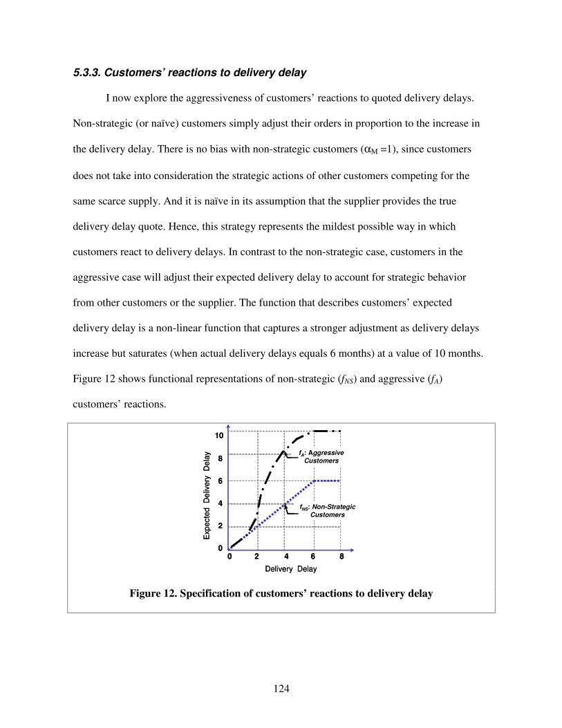
124

5.3.3. Customers’ reactions to delivery delay

I now explore the aggressiveness of customers’ reactions to quoted delivery delays.

Non-strategic (or naïve) customers simply adjust their orders in proportion to the increase in

the delivery delay. There is no bias with non-strategic customers (αΜ =1), since customers

does not take into consideration the strategic actions of other customers competing for the

same scarce supply. And it is naïve in its assumption that the supplier provides the true

delivery delay quote. Hence, this strategy represents the mildest possible way in which

customers react to delivery delays. In contrast to the non-strategic case, customers in the

aggressive case will adjust their expected delivery delay to account for strategic behavior

from other customers or the supplier. The function that describes customers’ expected

delivery delay is a non-linear function that captures a stronger adjustment as delivery delays

increase but saturates (when actual delivery delays equals 6 months) at a value of 10 months.

Figure 12 shows functional representations of non-strategic (fNS) and aggressive (fA)

customers’ reactions.

8

00 8

6

2

2 6

4

4

Delivery Delay

Exp

ecte

d D

eliv

ery

Del

ay

10

fA: Aggressive Customers

fNS: Non-StrategicCustomers

8

00 8

6

2

2 6

4

4

Delivery Delay

Exp

ecte

d D

eliv

ery

Del

ay

10

fA: Aggressive Customers

fNS: Non-StrategicCustomers

Figure 12. Specification of customers’ reactions to delivery delay

125

In the following set of tests, I run the model under a general function, for customer

reactions to delivery delay, which is a linear combination of the polar functions (non-strategic,

fNS, and aggressive, fA).

ANSCR fwwff )1( −+= (24)

where w corresponds to the weight of function (fNS) and w∈ [0,1].

Figure 13(a) shows backlogs under each customer response. First, it is important to

notice that even under customers’ non-strategic case (w1 = 1) – no strategic ordering among

customers – backlog and the expected delivery delay still increase. This result is analogous to

the case when capacity is fixed. However, backlogs returns to the equilibrium level gradually

rather than decreasing sharply as do systems with strategic ordering. Second, the

aggressiveness of customers’ competition matters. In the strategic case (w1 = 0.5), a maximum

customer bias increases the expected delivery delay by 25% (from 6 to 8 months), causing

backlogs to increase by a factor of four. In the aggressive case (w1 = 0), customer reactions

cause expected delivery delays to increase by 66% (from 6 to 10 months), leading to an

increase in backlogs by a factor of seven.

012

2436

4860

0

100

200

300

400

500

600

700

800

Time (Months)

Customer Reactions

Backlog

700-800600-700500-600400-500300-400200-300100-2000-100

10

0.5

012

2436

4860

0

100

200

300

400

500

600

700

800

Time (Months)

Customer Reactions

Backlog

700-800600-700500-600400-500300-400200-300100-2000-100

700-800600-700500-600400-500300-400200-300100-2000-100

10

0.5

012

2436

4860

100

120

140

160

180

Time (Months)

Customer Reactions

Capacity

160-180140-160120-140100-120

100.5

012

2436

4860

100

120

140

160

180

Time (Months)

Customer Reactions

Capacity

160-180140-160120-140100-120

160-180140-160120-140100-120

100.5

Figure 13. Supplier (a) backlog and (b) capacity to different customers’ reactions.

126

Figure 13(b) shows the supplier’ s capacity under different customers’ strategic

scenarios. In the non-strategic case (w1 = 1) the supplier increases capacity by 5% and in the

aggressive scenario (w1 = 0) by more than 65%. Thus the supplier accumulates much more

capacity than desired when customers pursue a very aggressive strategy to obtain their orders.

Customers’ responses may be interpreted in at least two ways. One possibility is that it

represents individual customers’ responses to shortages. Hence, individuals with more

aggressive natures may respond in a more emphatic way than other individuals, inflating their

orders more. In this context, the supplier may choose to focus on managing the orders of

aggressive customers, to prevent the reaction of other competitor customers.

Another possibility is that the responses capture the competitive environment that

customers face. More aggressive responses can be expected in more competitive

environments. In that case, we would expect to see more pronounced demand bubbles in

industries where the amount of competition among players is intense. Furthermore, since the

number of players can influence the nature of the competition, limiting the number of

customers that a supplier partners with may help suppliers mitigate order inflation.

Alternatively, suppliers may choose to give priority to preferred customers, preventing them

from being affected by shortages when they occur.

5.4. Multivariate Sensitivity Analysis

This section investigates the sensitivity of the model behavior with respect to changes

in multiple parameters simultaneously. Single parameter sensitivity provides valuable insights

about the impact of specific variables on model behavior, but it is limited for two reasons.

First, the model is highly nonlinear; sensitivity to multiple parameters cannot be simply

superimposed as in linear systems. Single parameter sensitivity ignores interaction effects.

127

Second, it does take into consideration prior knowledge about specific variable uncertainty.

Multivariate sensitivity takes both aspects into consideration. Table 1 provides a list of

parameters, uniformly distributed within a specified range that serves as input for the Monte-

Carlo (multivariate) simulation. The model is simulated 5000 times with independently

randomly selected parameter values from the uniform distributions.

Table 1. Parameters and range of uniform distributions

Parameter Acronym Units Min Base Max

Time to Build Capacity (τK) months 3 12 24

Time to Cancel Excess Orders (τC) months 0.25 3 6

Time to Perceive Delivery Delay (τDD) months 0.25 1 6

Time to Form Demand Expectation (τE) months 1 2 3

Time to Adjust Channel Backlog (τB) months 1 3 6

Weight of Non-Strategic Function (w) dmnl 0 0.5 1

The wide range of values for parameter inputs leads to substantial variance in other

key variables, such as supplier backlog and capacity. Figure 14 shows the confidence bounds

for the supplier’ s backlog and capacity. First, despite the wide range in input parameter

values, the system behavior for the supplier’ s backlog and capacity always follow a pattern of

overshoot-and-collapse. A smooth increase for the supplier’ s backlog and capacity takes place

when customers are myopic (do not over-order), the time to build capacity is short, and the

time to cancel orders is long. In contrast, a sharp increase and collapse in order backlog and

large capacity investment takes place when customers are aggressive, the time to build

capacity is long, and the time to cancel orders is short. Second, the result of a pulse input in

demand is a single overshoot-and-collapse in the suppliers’ backlog, driven by the positive

loop of customers’ reactions. This behavior contrasts to the oscillatory behavior of the beer

game, originating mainly from the structure of the supply chain. The characteristic

128

oscillations of the “ Forrester Effect” (Forrester 1961) cannot be obtained by a model that

captures solely customers’ reactions to supply shortages. To generate the oscillatory behavior,

the model structure would need to capture the negative feedbacks with long delays associated

with the supply chain inventory management. The reinforcing loops examined here would

destabilize the oscillations that would be produced by the missing structure.

1500

1000

500

00 25 50 75 100

Time (Months)

Backlog

50%75%

95%100%

Base

1500

1000

500

00 25 50 75 100

Time (Months)

Backlog

50%75%

95%100%

Base

400

300

200

100

00 25 50 75 100

Time (Months)

50% 75% 95% 100%

Base

Capacity400

300

200

100

00 25 50 75 100

Time (Months)

50% 75% 95% 100%

Base

Capacity

Figure 14. Multivariate sensitivity for supplier’s (a) backlog and (b) capacity

Table 2 provides summary statistics from the Monte-Carlo simulations for outcome

variables of the system. In the extremes, a one year 10% increase in customer demand can

generate more than a doubling in capacity and a nine-fold increase in order backlog.

Table 2. Uncertainty in Supplier’s Backlog and Capacity

Parameter (t=30) Min Max Mean Median Norm. Std Dev

Deterministic

Available Capacity (K) 101 218 111 105 13.2 124

Order Backlog (B) 13 916 248 175 174 444

Note: Values reported for 5000 simulations at time t =30. The deterministic case reports values from the base case.

5.5. Optimal Capacity Trajectory

The desired capacity trajectory is a control heuristic that takes into consideration the

costs associated with customer satisfaction (low delivery delays), order cancellations, and new

capacity to set a monthly capacity target. The criterion to evaluate the optimal capacity

129

trajectory is maximization of net present value of cumulative discounted profits (CDP) over

the simulation period, with a discount rate (r). Actual capacity (K) adjusts to the desired level

(K*) with a third-order Erlang lag (λ), with an average time constant of one year.

πrtePDC −=� (25)

),( * λKLK = (26)

Profits (π) are revenues (R) minus total costs (TC). The former is given by the product

of shipments (S) and price (p). Price is set at a constant markup (m) above total unit costs

(UT). Total costs are the sum of variable costs (Cv), associated with production (S); fixed costs

(Cf), associated with capacity (K); and customer dissatisfaction costs (CD).

TCR −=π (27)

TUmSR ⋅+⋅= )1( (28)

Variable costs (Cv) are a function of variable unit costs (Uv) and production (S), where

variable unit costs (Uv) are a fraction (fv) of total unit costs (UT).

SUC vv ⋅= (29)

Tvv UfU ⋅= (30)

Fixed costs (Cf) are a function of capacity (K) and fixed unit costs (Uf), where the

latter are a fraction (1-fv) of total unit costs (UT).

KUC ff ⋅= (31)

Tvf UfU ⋅−= )1( (32)

Suppliers also consider a cost of customer dissatisfaction (CD) that is proportional (α)

to unit variable costs (Uv) and the fraction of shipments delivered with an excess delivery

delay.

130

))))(

()(,0(()()( 2*

*

DDDDtDD

tSMAXUtCD v−⋅⋅⋅= α (33)

I investigate the optimal capacity trajectory for two cases: when suppliers take into

consideration customer dissatisfaction costs (α=1) and when they do not (α=0). Figure 15

shows the results of the optimization runs. Graph 15 (a) shows the optimal trajectory for the

two scenarios compared to the base case. When managers account for the cost of customer

dissatisfaction (α=1), they increase the capacity level early in the simulation to meet the pulse

increase in final customer demand. The additional capacity allows the supplier to meet

customer orders with a minor increase in backlog. After the pulse in demand occurs, the

supplier allows capacity to erode to the normal level. When managers do not consider the cost

of customer dissatisfaction (α=0), the relative cost of capacity is higher for the supplier,

resulting in delayed investments in new capacity. The capacity scarcity causes the supplier’ s

backlog to rise considerably, increasing the delivery delay. Customers make the problem

worse by inflating their orders, many of which will be cancelled later. The system behavior

deteriorates to a poor performance equilibrium, where the supplier carries a large order

backlog, leading to high delivery delay, and high cancellations.

The results are intuitive. When the supplier values customer satisfaction, it will invest

in capacity to maintain its backlogs and delivery delays at the desired levels. No demand

bubble takes place when the supplier incorporates the delivery delay costs in its cost

function.25 In contrast, when the supplier neglects customer dissatisfaction costs, it does not

invest in capacity due to its high costs. Failure to add necessary capacity causes it to operate

with excessive backlogs, long delivery delays, and large and frequent cancellations.

25 However, the current cost function does not account for costs associated with changes (acquisition/depletion) in capacity.

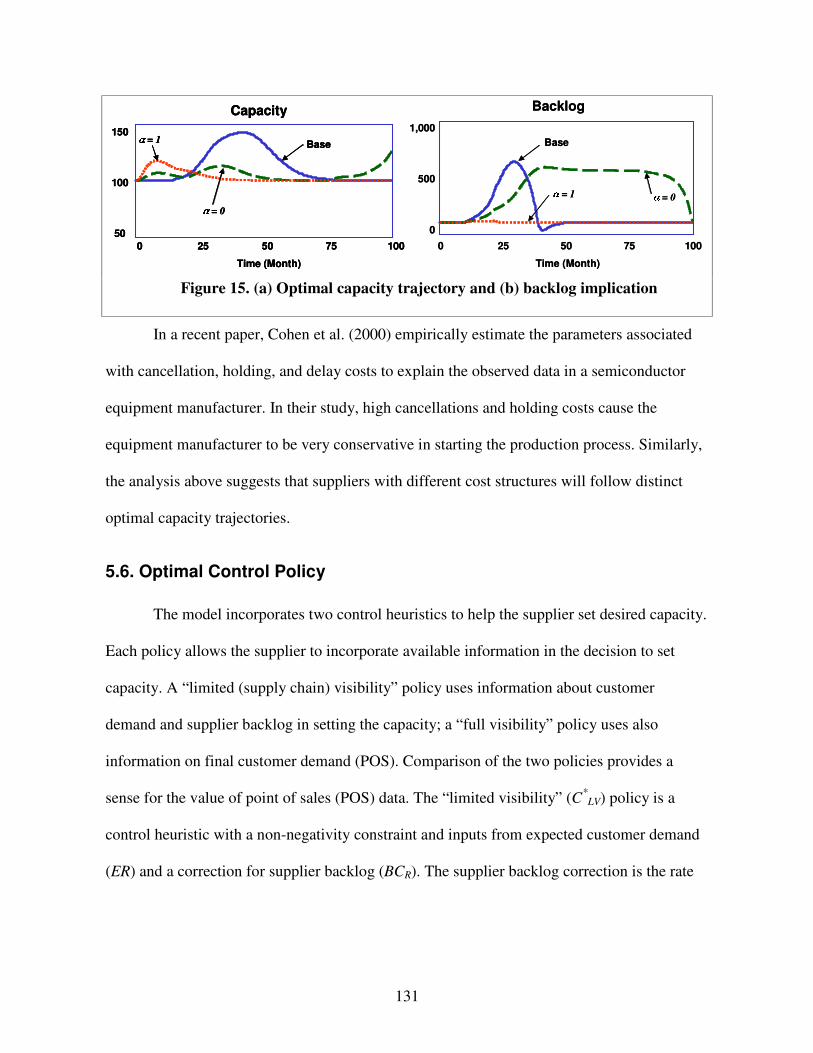
131

Capacity150

100

500 25 50 75 100

Time (Month)

� = 0

Base� = 1

Capacity150

100

500 25 50 75 100

Time (Month)

� = 0

Base� = 1

Capacity150

100

500 25 50 75 100

Time (Month)

� = 0

Base� = 1

Backlog1,000

500

00 25 50 75 100

Time (Month)

� = 0� = 1

Base

Backlog1,000

500

00 25 50 75 100

Time (Month)

� = 0� = 1

Base

Figure 15. (a) Optimal capacity trajectory and (b) backlog implication

In a recent paper, Cohen et al. (2000) empirically estimate the parameters associated

with cancellation, holding, and delay costs to explain the observed data in a semiconductor

equipment manufacturer. In their study, high cancellations and holding costs cause the

equipment manufacturer to be very conservative in starting the production process. Similarly,

the analysis above suggests that suppliers with different cost structures will follow distinct

optimal capacity trajectories.

5.6. Optimal Control Policy

The model incorporates two control heuristics to help the supplier set desired capacity.

Each policy allows the supplier to incorporate available information in the decision to set

capacity. A “ limited (supply chain) visibility” policy uses information about customer

demand and supplier backlog in setting the capacity; a “ full visibility” policy uses also

information on final customer demand (POS). Comparison of the two policies provides a

sense for the value of point of sales (POS) data. The “ limited visibility” (C*LV) policy is a

control heuristic with a non-negativity constraint and inputs from expected customer demand

(ER) and a correction for supplier backlog (BCR). The supplier backlog correction is the rate

132

that the supplier adjusts the actual backlog to its desired level, given by the product of

expected shipments and the target delivery delay.26 27

),0(*RLV BCERMAXC ⋅−⋅= γβ (34)

The “ full visibility” (C*FV) policy not only incorporates the information on backlog

correction and expected customer demand, but also information on final customer demand

(d).

)])1([,0(*RFV BCdERMAXC ⋅−⋅−+⋅= γββ (35)

The control policy optimization runs seeks optimal values for the parameters β and γ,

in the two policy heuristics. While the two heuristics may not include the true optimal

trajectory for desired capacity, the heuristics are flexible and can be easily interpreted in terms

of concepts (direct customer demand, final customer demand, and supplier backlog

correction) meaningful to the supplier. The same cost structure and criterion to evaluate

optimality used in the previous section are used in this section. The search is performed by a

gradient-free hill-climbing algorithm (Ventana Systems 1998). I investigate the two optimal

control heuristic for two different cost structure: when suppliers consider customer

dissatisfaction costs (α=1) and when they do not (α=0). Figure 16 shows the evolution of

parameters β and γ in the full visibility case for various levels of customer aggressiveness.

26 The supplier’ s desired backlog is different from the channel’ s desired backlog. The latter accounts for customer’ s desired backlog level, which incorporates phantom orders, and is determined by the product of customer’ s demand and the expected delivery delay. The product of expected shipments to the target delivery delay determines the former. 27 The backlog correction is subtracted in the equation to capture the need to add capacity when the actual backlog is greater than desired (BCR < 0); and, reduce it when backlog is lower than desired (BCR > 0).

133

Policy Control Heuristic- Full Visibility

0

0.2

0.4

0.6

0.8

1.0

0% 20% 40% 60% 80% 100%

Aggressiveness Weight

E�D = 0

E�D = 1

J�D = 0

J�D = 1

Policy Control Heuristic- Full Visibility

0

0.2

0.4

0.6

0.8

1.0

0% 20% 40% 60% 80% 100%

Aggressiveness Weight

E�D = 0

E�D = 1

J�D = 0

J�D = 1

Figure 16. Optimal control heuristics

When suppliers do not consider the cost of customer dissatisfaction (α=0), that is,

they place more importance on their fixed and variable costs, the supplier fully incorporates

the information on final customer demand (β =0) to base capacity decisions. Suppliers always

benefit from knowing final customer regardless of the aggressiveness of direct customer

competition (order inflation). In addition, the supplier does not consider the backlog

correction when setting capacity. While the supplier uses POS data to base capacity decisions,

it will not meet direct customer demand. A demand bubble is likely to take place when

suppliers do not consider the cost of customer dissatisfaction (α=0), just as in the optimal

trajectory case for (α=0).

In contrast, when the supplier accounts for the cost of customer dissatisfaction (α=1),

it considers the backlog correction when setting capacity. Since backlogs influence the

delivery delays, and delivery delays influence costs, by taking the backlog correction into

account the supplier can minimize its costs. In addition, the supplier, accounting for customer

dissatisfaction costs (α=1), considers the information on POS data (β =0) only when direct

134

customers are not too aggressive (w ≥ 0.5). If direct customers are very aggressive (w � 0.4),

the supplier sees little value for the POS data (β =1). The rationale for not using final

customer demand (POS) information when customers are too aggressive is that the data does

not provide information that will help the supplier satisfy direct customer demand. Ironically,

suppliers base capacity decisions on direct customer demand, exactly when direct customers

inflate orders more aggressively, and when POS data would be most valuable.

When direct customers are not aggressive (w ≥ 0.5) and customer dissatisfaction costs

are accounted for (α=1), the supplier does not use POS data (β =1) to base capacity decisions.

Hence, the supplier meets demand for its direct customers and is capable of avoiding a

demand bubble, just like the optimal trajectory case for (α=0). When direct customers are

aggressive (w ��KRZHYHU��WKH�VXSSOLHU�XVHV�326�GDWD��β =0) to base capacity decisions,

failing to meet direct customer demand, and generating a demand bubble.

6. Discussion

In this paper, I considered the phenomenon of bubbles in demand that can take place

when customers compete for the supply of scarce products. The paper contributes to the

understanding of the phenomenon by providing a comprehensive causal map of the

relationships leading to customers’ inflation of orders. In addition, I provide a formal model

for one of the possible customers’ reinforcing loops: the Ordering Ahead (R1) loop. I obtain

closed form solutions to the behavior of supplier backlogs, assuming that supplier capacity is

fixed. Even when non-strategic customers order the exact amount to compensate for an

increase in delivery delays, the system performance decreases, leading to higher backlogs and

longer delivery delays. If customers behave strategically and the supplier capacity is fixed, the

135

analysis suggests that a transient shortage in supply can drive the supplier out of stability,

leading to high backlogs and delivery delays. The supplier’ s ability to bring capacity online

can help reduce the size of the bubble. However, the supplier still goes through a transient

period of low performance, as it takes time to bring new capacity online. When the additional

capacity becomes available and customers start receiving their orders, the bubble busts. The

bust is characterized by a period of order cancellations followed by a period of reduced

demand, as customers deplete their excess inventories. Suppliers are left with excess

inventories and capacity greatly exceeding the original amount of product in short supply. For

instance, a 10% transient (one year) increase in customer demand can induce capacity

increases on the order of 30% to balance customer’ s order inflations and backlogs can

increase by 300% relative to its equilibrium level.

Furthermore, the faster the supplier can add new capacity the lower the impacts of the

bubble, that is, it will require less capacity and it will face a shorter period of low performance

with lower backlogs and shorter delivery delays. Hence, the ability to bring capacity online

quickly helps suppliers prevent the growth in the bubble. However, capacity flexibility alone

may not be a sustainable way to deal with demand bubbles. Even when they limit the impact

of the demand bubble, suppliers are left with excess capacity. This effect is particularly

important when adequate time constants for the depreciation of capacity are taken into

consideration. Since a rapid introduction of new capacity can significantly reduce the size of

the demand bubble, it is important to consider flexible strategies for quickly bringing new

capacity online.

In addition, the analysis suggests that an important leverage point in the system is

customer’ s perception delay of supplier’ s delivery delay. When the supplier provides real-

136

time information about delivery delays to customers, the system is highly unstable because

customers react instantaneously to the readily available information. If customers see an

increasing delivery delay, they will respond rapidly and will inflate their orders to hedge

against shortages, only making the situation worst. In contrast, when the supplier provides

information about delivery delays with a long time delay to customers, the system is more

stable because it will take time before customers over-react, giving the supplier an

opportunity to act – speeding up production, increasing overtime, increasing safety stocks of

raw material and components, and bringing up new capacity online – to reduce delivery

delays. Interestingly, the idea of suppliers providing delayed information about delivery

delays and inventory availability goes in direct opposition to the current industry trend to

introduce information systems providing real-time information to all parties in the supply

chain. Unfortunately, these real-time information systems may be introducing a great deal of

instability, leading to the creation of larger than ever demand bubbles. While companies claim

to have saved millions of dollars in purchasing and ordering operations, the costs associated

with over-ordering may far exceed the savings generated from the accurate processing of

orders.

Interpreting the aggressiveness of customers’ responses as a measure of market

competitiveness, the results suggest that more pronounced demand bubbles would take place

in industries where competition among customers is intense. To avoid the impact of

competition, suppliers may choose to give priority to preferred customers or to limit the

number of customers that they will work with. In addition, investigation of the optimal

capacity trajectory suggests that occurrence of demand bubbles are predicated on supplier’ s

cost structure. When the supplier values customer satisfaction (e.g. it incorporates the delivery

137

delay costs in its cost function), no demand bubble takes place. The supplier invests in

capacity to maintain its backlogs and delivery delays at the desired levels. In contrast, when

the supplier does not account for customer dissatisfaction costs, it does not investment in

capacity due to the associated high (fixed and variable) costs. Failure to add necessary

capacity causes the supplier to operate in a situation of excessive backlogs, long delivery

delays, and large and frequent cancellations.

A number of researchers (e.g. Kaminsky and Simchi-Levi 1996, Gupta, Steckel and

Banerji 1998) have analyzed policies (e.g., centralizing ordering decisions, reducing order

lead-times, and sharing Point-of-Sales (POS) data) for reducing demand variability.

Particularly important to demand bubbles is the availability of POS data. If suppliers had

access to such data it is arguable that they would not be facing such harsh conditions since

they could distinguish true demand from customer-inflated demand. However, it is unrealistic

to expect that customers plagued by shortages would be willing to share such information

with their suppliers in the first place, since it would limit their ability to obtain more products

when needed. In addition, those customers who might be willing to share such information

would potentially risk receiving less than others who would be inflating their orders. This

situation could be improved, however, if the supplier gave priority to those customers willing

to share POS data.

Testing a control heuristic for the supplier with full supply chain visibility suggests

that the value of POS data depend ultimately on the nature of supplier costs and customer

competition. Suppliers fully incorporate POS data on capacity decisions when their cost

structure does not account for customer dissatisfaction costs. However, when suppliers

account for customer dissatisfaction costs, POS data is only used when customers are not too

138

aggressive. When customer competition is too fierce, POS data does not provide information

that will help the supplier to satisfy valuable customer demand. Ironically, suppliers base

capacity decisions on direct customer demand, exactly when customers inflate orders more

aggressively and when POS data would be most valuable.

In summary, this paper contributes to the discussion of order amplification in supply

chains due to supply shortages. It offers a comprehensive causal map of the relationships

leading to customers’ inflation of orders and a formal mathematical model of one reinforcing

loop of customers’ responses. It provides a closed form solution to the behavior of supplier

backlogs when the supplier has fixed capacity and an analysis of the simulation when capacity

is flexible. Finally, parameter sensitivity analysis explores how the model behavior changes

due to parameter changes, leading to a deeper understanding of the long-term impacts of

demand bubbles and policies solutions that may mitigate their impacts.

7. References

Adelman, D. 2001. “ First Loss Sets Gloomy Tone at CISCO.” Wall Street Journal. May 9, B1.

Anderson, E. and C. Fine. 1999. “ Business Cycles and Productivity in Capital Equipment Supply Chains.” In Tayur et al. Quantitative Models for Supply Chain Management. Kluwer Academic Publishers, Norwell, MA.

Baljko, J.L. 1999. “ Expert Warns of ‘Bullwhip Effect’ .” Electronic Buyers’ News. July 26, p. 5

Blumenstein, R. 1996. “ Autos: How do you get a hot GMC Suburban? You wait for a computer to dole one out.” Wall Street Journal. April 10, B1.

Boslet, M. 1998. “ Intel Experiences Some Shortages in Pentium II Chips.” Wall Street Journal. August 14, B5.

Cachon, G., and M. Lariviere. 1999a. “ Capacity Allocation Using Past Sales: When to Turn-and-Earn.” Management Science. 45(5): pp. 685-703.

139

Cachon, G., and M. Lariviere. 1999b. “ Capacity Choice and Allocation: Strategic Behavior and Supply Chain Performance.” Management Science. 45(8): pp. 1091-1108.

Cachon, G. 1999. “ Managing Supply Chain Demand Variability with Scheduled Ordering Policies.” Management Science. 45(6): pp. 843-856.

Cachon, G., and P. Zipkin. 1999. “ Competitive and Cooperative Inventory Policies in a Two-Stage Supply Chain.” Management Science. 45(7): pp. 936-953.

Chen, F. 1999. “ Decentralized Supply Chains Subject to Information Delays.” Management Science. 45(8): pp. 1076-1090.

Chen, F., Z.Drezner, J.Ryan, and D.Simchi-Levi. (2000) “ Quantifying the Bullwhip Effect in a Simple Supply Chain: The Impact of Forecasting, Lead Times, and Information.” Management Science, 46(3), pp. 436-443.

Clancy, H. 2001. “ Brick Wall Effect.” The Newsweekly for Builders of Technology Solutions. April 16. Issue 941: p. 24.

Cohen, M., T. Ho, J. Zen, and C. Terwiesch. 2001. “ Measuring Imputed Costs in the Semiconductor Equipment Supply Chain.” Wharton School of Business working paper, University of Pennsylvania.

Croson, R. and K. Donohue. 2000. “ Behavioral Causes of the Bullwhip Effect and the Observed Value of Inventory Information.” Wharton School of Business working paper, University of Pennsylvania.

Diehl, E. and J.D. Sterman. 1995. “ Effects of Feedback Complexity on Dynamic Decision Making.” Organizational Behavior and Human Decision Processes. 62(2): pp. 198-215.

Foremski, T. 1999. “ Intel struggles to meet strong demand for chips,” Financial Times (London), November 18, pg. 42.

Federgruen, A. 1993. “ Centralized Planning Models for Multi-Echelon Inventory Systems under Uncertainty.” Handbook in Operations Research and Management Science- Vol. 4: Logistics of Production and Inventory, S.C. Graves, et al. (Eds.), Elsevier, Chapter 3, pp. 133-173.

Forrester, J.W. 1958. “ Industrial Dynamics – A Major Breakthrough for Decision Makers.” Harvard Business Review. 36(4), pp. 37-66.

Forrester, J.W. 1961. Industrial Dynamics. Cambridge, MA: Productivity Press.

Forrester, J.W. 1968. Principles of Systems. Cambridge, MA: Productivity Press.

Forrester, J.W. 1968. “ Market Growth as Influenced by Capital Investment.” Industrial Management Review. 9(2): p. 83-105.

140

Gaither, C. 2001. “ Intel Beats Forecast; Warns of Revenue Shortfall,” The New York Times, January 17, C1.

Greek, D. 2000. “ Whip Hand.” Professional Engineering. May 24. 13(10): p. 43.

Gupta, S., J. Steckel and A. Banerji. 1998. “ Dynamic Decision Making in marketing Channels: An Experimental Study of Cycle Time, Shared Information and Consumer Demand Patterns.” Stern School of Business working paper, New York University.

Hwang, S. L. and L. Valeriano. 1992. “ Marketers and consumers get the jitters over severe shortages of nicotine patches.” Wall Street Journal. May 22, B1.

Kaminsky, P. and D. Simchi-Levi. 1998. “ A New Computerized Beer Game: A Tool for Teaching the Value of Integrated Supply Chain Management.” In Supply Chain and Technology Management. H. Lee and S.M. Ng (eds), The Production and Operations Management Society. 216-225.

Kahneman, D. and A. Tversky. 1982. “ The Simulation Heuristic.” In Kahneman, D. et al.. Judgment Under Uncertainty: Heuristics and Biases. Cambridge University Press, Cambridge.

Lawrence, D. 1996. “ GM test allocation change: More makers scrap turn-and-earn plan.” Automotive News. February 12, 142.

Lee, H., Padmanabhan, V, and Seungjin Whang. 1997a. “ Information Distortion in a Supply Chain: The Bullwhip Effect.” Management Science, 43(4): pp. 546-558.

Lee, H., Padmanabhan, V, and Seungjin Whang. 1997b. “ The Bullwhip Effect in Supply Chains.” Sloan Management review, Spring: pp. 93-102.

Lee, H. and S. Wang. 1999. “ Decentralized Multi-Echelon Supply Chains: Incentives and Information.” Management Science. 45(5): pp. 633-640.

Li. L. 1992. “ The Role of Inventory in Delivery Time Competition.” Management Science. 38(2): pp. 182-197.

Mass, N. 1975. “ Economic Cycles: An Analysis of Underlying Causes.” Cambridge, Mass. Wright-Allen Press.

McWilliams, G. 2000. “ Shortages of an Intel Microprocessor Creates Backlogs, Headaches.” Wall Street Journal. August 23, B1.

Merton, R. K. 1948. “ The self-fulfilling prophecy.” Antioch Review. 8: p.193-210.

Morecroft, J.D. 1980. “ A Systems Perspective on Material Requirements Planning.” Decision Sciences. 14: pp. 1-18.

141

Morecroft, J.D.W. 1983. “ System Dynamics: Portraying Bounded Rationality.” Omega. 11(2): p. 131-142.

Morecroft, J.D.W. 1985. “ Rationality in the Analysis of Behavioral Simulation Models.” Management Science. 31(7): p. 900-916.

Richardson, G. and A. Pugh. 1980. Introduction to System Dynamics Modeling with Dynamo. Productivity Press, Portland, Oregon.

Savage, M. 1999. “ Component aftershock hits channel.” Computer Reseller News. October 18.

Schwartz, J. 2001. “ Business on Internet Time: The Ups Are Fast. The Downs Could Be Even Faster.” The New York Times. March 30, C1.

Singhal, V. and K. Hendricks. 2002. “ How Supply Chain Glitches Torpedo Shareholder Value.” Supply Chain Management Review. January/February. pp.18-33.

Sterman, J.D. 1989a. Modeling Managerial Behavior: Misperceptions of Feedback in a Dynamic Decision Making Experiment. Management Science. 35(3): p. 321-339.

Sterman, J.D. 1989b. “ Misperceptions of Feedback in Dynamic Decision making.” Organizational Behavior and Human Decision Sciences, 43, 3:301-335.

Sterman, J., N. Repenning and F. Kofman. 1997. “ Unanticipated Side Effects of Successful Quality Programs: Exploring a Paradox of Organizational Improvement.” Management Science, April, 503-521.


Zarley, C. and K. Damore. 1996. “ Backlogs plague HP: Resellers place phantom orders to get more products.” Computer Resellers News. May 6, 247.

143

Investigating the Causes of Returns in the Seed Supply Chain

Paulo Gonçalves



[email protected]

Abstract:

Hoarding is a common occurrence during shortages of “ hot” products in industries ranging from oil to toys and from computers to pharmaceuticals. Often the induced shortage due to hoarding is much stronger than the original trigger. This paper investigates the impact of dealer hoarding on generating large amounts of seeds returned to a seed corn supplier in the agribusiness industry. To understand the mechanisms leading to seed corn hoarding and returns, we build a formal model of seed hoarding in the agribusiness supply chain. Our insights suggest that dealer hoarding and subsequent seed returns result from the interplay between supply chain characteristics (e.g. timing of information availability and quality of dealers’ orders) and human decision making (e.g. salespeople’ s effort allocation decisions and managers’ pressure). In addition, a number of supplier actions can intensify dealers hoarding behavior, worsening the problem. Our analysis suggests several policies capable of effectively reducing the volume of returns. Key words:

Seed returns, supply chain management, over-ordering, agribusiness industry, system dynamics, and simulation.

145

1. Introduction

Hoarding – storing up supplies – is a common occurrence during shortages of “ hot”

products, ranging from the basic (e.g. gasoline and food) to the sophisticated (e.g.

pharmaceuticals and new technology products). For instance, hoarding and gasoline shortages

took place during the OPEC oil embargo against the United States in 1973, the oil supply

reduction after the Iranian revolution in 1979, and in Britain and Europe in 2001. Such

periods were marked by service stations rationing the maximum amount of gasoline

purchased per customer and by panic consumer buying, with anxious consumers queuing for

hours in attempts to top off their tanks. Some analysts reported that the hoarding was worse

than the oil embargo itself. One example of the effects of hoarding was the illegal storage of

the fuel (Anonymous 1974). In December 1999, fearing that Y2K problems would interrupt

food supplies, overcautious customers stocked up on water, food and batteries (Weiss 1999).

More recently, following the anthrax attacks of 2001, customers in the U.S. rushed to drug

stores to hoard supplies of Cipro, causing generalized shortages of the drug (Petersen 2002).

In all such cases, customers hoarded products to hedge against the expectation of shortages,

often causing impacts much larger than if real shortages took place. Indeed, even the initially

false rumor of shortages can trigger hoarding – a classic example of a self-fulfilling prophecy

(Merton 1948).

This paper investigates the causes of corn seed hoarding in the agribusiness supply

chain, leading to excessive seed corn returns to a major U.S. seed supplier. Excessive returns

impose substantial costs on seed suppliers due to transportation, retesting, reconditioning,

repackaging, discards due to poor storage, and discards due to lifetime expiration. By law,

returned seeds must be retested and repackaged even when storage conditions at dealers’

146

warehouses are satisfactory. Not all returned seeds can be reconditioned, however. Often,

returned seeds need to be discarded due to poor storage conditions. Furthermore, corn has a

maximum three-year shelf-life, after which it has to be discarded. Excessive returns also drive

indirect costs associated with excess production capacity required to accommodate a large

volume of returns.

The agribusiness industry traditionally faces returns of 15% of the total seeds shipped

to dealers. The seed supplier tolerates some level of returns, since demand is uncertain. In

addition, the seed supplier perceives the losses due to returns as much lower than the gains

due to potential sales and market share. Seed suppliers often encourage dealers to overstock to

stimulate opportunistic sales or to prevent competitors from having shelf-space for their

products. Dealers also benefit from returns. Seed production takes place months in advance of

grower demand, often resulting in a limited supply of specific hybrids. To hedge against

shortages of high performing hybrids, dealers often place their orders early in the selling

season, and also inflate them. If, later on, grower demand materializes, dealers benefit from

their inflationary ordering behavior. If it does not, they can return any excess inventory at no

additional costs. Hence, both the seed supplier and dealers can benefit from over-ordering and

subsequent returns.

While the benefits (opportunistic sales and limited competitor shelf-space) associated

with overstocking seeds at dealers exist, the direct and indirect costs may far outweigh them.

In particular, the seed supplier, I investigated had returns twice as high as the industry

average, and direct costs associated with corn seed returns on the order of 10% of revenues

(about $20 million per year). Our interviews revealed that the ratio of produced seeds to sales

equaled 1.7, that is, the total volume of seeds produced would be sufficient to sustain almost

147

twice as many sales, hinting at significant indirect costs (excess capacity) that may far

outweigh the direct costs of returns.

To understand the mechanisms leading to seed hoarding and returns, we build a formal

model of seed hoarding in the agribusiness supply chain. By capturing the dynamics of

salespeople’ s effort allocation between competing tasks during the selling season, the model

yields a number of insights into the process that lead to seed hoarding and returns. Our model

rests on quantitative and qualitative data gathered from a three-month in-depth study of sales,

services, planning, operations, logistics, and order processes at the company site, a major U.S.

supplier of corn and soybean seeds. During our field work, we conducted about thirty semi-

structured interviews with company and dealer managers. Eighty percent of the interviewees

were managers at the seed supplier in charge of operations, logistics, quarterly initiatives,

production planning, demand forecasting, sales, order processing, and supply chain

management. The other twenty percent of interviewees were managers working at either

agribusiness or seed-only dealers. The former sells seeds, herbicides, and other agribusiness

products directly to growers and smaller dealers. The latter sells only seeds, primarily to

growers. The quantitative and qualitative data support the development of a system dynamics

model of the problem, providing crucial information on managers’ and salespeople’ s decision

heuristics for performing daily activities, causal relationships among different areas of the

business, and specific data on monthly returns and net sales, weekly requests and shipment

rates, sales quotas, and fraction of such quotas met by salespeople.

Model results suggest that dealer hoarding and excess seed returns result from the

interplay between supply chain characteristics (e.g. timing of information availability and

quality of dealers’ orders) and human decision making (e.g. salespeople’ s effort allocation

148

decisions and managers’ pressure). Most important, seed hoarding and excess returns can

generate a self-reinforcing process. Returns from last season influence dealers’ ordering

decisions this season, leading to hoarding and further returns. After having trouble getting the

desired seeds last season, dealers learn to inflate their orders in the coming season to improve

their chances of meeting farmer’ s needs. In addition, actions by the supplier’ s managers can

intensify dealers’ hoarding behavior, worsening the problem. While it is difficult for the seed

supplier to distinguish actual grower orders from dealers’ inflated orders, salespeople’ s effort

in positioning the seeds can help. However, salespeople’ s must also spend effort pushing

seeds to meet revenue targets. When pressure to meet these revenue targets increases,

salespeople allocate more effort to pushing seeds to dealers to the detriment of positioning

them adequately. Managerial pressure to meet end-of-year revenue targets shifts salespeople’ s

effort allocation from positioning to pushing seeds, leading to seeds located at dealers without

grower demand and, ultimately, higher seed returns.

The paper proceeds as follows. The next section describes the seed supply chain and

relates to the relevant literature. Section 3 describes the model and the evidence for its main

assumptions. Section 4 contains the base simulation run, results, and sensitivity analysis

followed by policy analysis in section 5. We conclude with a discussion of insights and areas

for further research.

2. Seed Supply Chain

The seed supplier markets hundreds of corn SKUs every year. Corn hybrids are

genetically engineered to provide insect protection, herbicide resistance, and specific

performance for local weather conditions. Every year the supplier withdraws many old

products and introduces several new ones. Product life-cycles are short. The supplier must

149

also manage high demand and supply uncertainty. Supply uncertainty is highly dependent on

weather variability, uncertain yields, uncertain growing (e.g. insect) conditions, and long

delays in seed production. Demand uncertainty depends heavily on farmers’ experience in the

previous growing season. In many ways, the challenges faced by the seed-corn industry

resemble those of the electronics and computer industries.

Dealer 1

Dealer n…

orders

orders

seeds

seeds

seeds

orders

seeds

GrowersSeed Company

Dealer 1

Dealer n…

orders

orders

seeds

seeds

seeds

orders

seeds

GrowersSeed Company

Figure 1. Distribution channel for the seed company

In a typical agribusiness supply chain, the seed supplier sells seeds to dealers, who

then resell them to growers (Figure 1). Seed production takes place months in advance of

grower demand, often resulting in a limited supply of specific hybrids. To secure the hybrids

believed to be in high demand, dealers’ inflate their orders and place them early in the selling

season, before grower demand materializes. In turn, growers base their ordering decision on

hybrids that perform well in the current planting season. Hybrid performance, however, is

highly uncertain due to its dependency on weather conditions. Seed return policies in the

agribusiness industry encourage dealers to order seed hybrids despite the uncertainty in

grower demand.

Donohue (1996) suggests that manufactures using a returns policy (e.g. a rebate on

unsold items) can often influence retailers to place larger orders. Webster and Weng (2000)

corroborate this finding advising that while “ returns policies can increase the ‘upside

150

potential’ of manufacturer profit by encouraging retailers to order more, they also introduce

‘downside exposure’ through high rebate costs when demand is lower than expected.” Jones

et al. (2002, 2003) study the seed corn supply chain, but focus their attention on problems

associated with the timing of production. Since production decisions take place several

months before farmer decisions that determine demand, the product mix of available supply

often does not match farmer’ s needs. The authors suggest a second production in a region in a

different hemisphere, allowing for production decisions that incorporate information about

grower demand.

Padmanabhan and Png (1995, 1997) propose that an unlimited returns policy can have

an important role in increasing manufacturer’ s profit by increasing the intensity of retailer

competition. In contrast, Gonçalves (2002) provides a theoretical model where an increase in

retailer competition leads to inflationary ordering behavior, high order cancellation, and

higher manufacturer costs, due to excess capacity and finished goods inventory. Expanding on

that theoretical model, Shi’ s (2002) study of Cisco Systems showed how Cisco’ s actions –

such as favorable credit terms to retailers with the intention of promoting demand growth –

generated fierce retailer competition, a boom in retailer orders, further inflating the demand

bubble, and intensifying the subsequent bust, contributing to a record $2.2 billion inventory

write-off and massive layoffs.

Emmons and Gilbert (1996) investigate the role of returns to the maximization of

manufacturer’ s profit while incorporating retailers’ self-interested behavior into the

manufacturer’ s policy decision. The authors first maximize retailer profits and incorporate

those results in the supplier maximization problem. In sharp contrast to a model where fully

rational agents make optimization decisions, our paper assumes that managers have cognitive,

151

perception, information, psychological limitations on their rationality, presenting bounded

rationality as suggested in theory (Simon 1982, Cyert and March 1963, and others) and

observed empirically (Kahneman et al. 1982, Sterman 1989a, 1989b, Diehl and Sterman 1995,

Croson and Donohue 2000).28

3. Model Structure and Assumptions

This section details the causal mechanisms that lead to the increase in returns and four

main formulations, elicited during our fieldwork, describing agents’ (dealers, supplier’ s

managers, and salespeople) decisions and their intended rationality. While these decisions

may not be optimal, they reflect the heuristics used by agents on their everyday decisions.

Consider the timing of seed corn production and shipments in the North American

agribusiness industry (Figure 2). From January to March, the seed supplier chooses the mix

and volume of hybrids to produce. Once those decisions are made the mix of corn-hybrids

available in the following season is fixed. In April, growers plant the seeds produced and sold

by the supplier the previous season. The supplier also plants in April and late October is

harvesting time. After harvesting, the supplier must test, bag, and tag the corn-hybrids to get

them ready for delivery to dealers. While shipments to dealers start only in mid November,

dealers start placing their orders in mid September. Often dealers inflate their orders in an

attempt to get the corn-hybrids they believe will be in high demand by growers. Estimating

which hybrids will be in high demand, however, is not a trivial task due to the large number

of corn-hybrids and uncertainty associated with weather conditions. One difficulty arises from

the heuristics growers use to place their orders. Grower demand is highly influenced by the

28 Also see Morecroft (1983, 1985) and Sterman (1987) for further discussion of bounded rationality in simulation models.

152

performance of corn-hybrids in the recently harvested crop. Another difficulty arises from the

difficulty in determining grower demand. Dealers learn about grower demand only after

harvesting (by late December), when growers place the bulk of their orders. Growers often

delay receipt of seeds until they need them for planting at the end of March. At that time, the

seed supplier stops shipping corn-seeds to dealers. The majority of seed returns take place in

July, long after the selling season is over. Even when returns occur earlier in the season, they

often cannot be reconditioned in time to be sold in the current season, due to the time to re-

test, recondition, re-bag, and re-tag them.

Sept Oct Nov Dec Jan Feb MarMay JunApr Jul Aug

Plant Seeds Harvest

Apr

Seed Production Dealer Orders

Grower Orders

Shipments To DealersPlan

Production Seed Returns

Shipments To Growers

Sept Oct Nov Dec Jan Feb MarMay JunApr Jul Aug

Plant Seeds Harvest

Apr

Seed Production Dealer Orders

Grower Orders

Shipments To DealersPlan

Production Seed Returns

Shipments To Growers

Figure 2. Timing of corn seed production, orders and shipments

While the seed supplier starts shipping seeds to dealers in mid November, its fiscal

year ends in December. Therefore, any discrepancies between current and target revenues

must be met within that six-week period. During this period, salespeople face increased

pressure to meet the annual revenue target. As pressure increases, and given that dealers have

placed large orders in the previous months to hedge against potential shortages, salespeople

start to make phone calls requesting early delivery of existing orders. Dealers will tentatively

delay receipt of orders – since most growers will still not have firmed their orders – but given

that seeds can be returned later at no cost, dealers traditionally do not have a problem

153

accepting seeds sent early. Naturally, since growers have not placed their orders, salespeople

may be pushing corn-hybrids to dealers that lack the appropriate grower demand. As

salespeople effectively “ sell” more seeds, however, revenues increase, easing the pressure

from corporate headquarters. The managerial response of focusing salespeople’ s effort on

pushing seeds has the desired consequence of increasing revenues in the short run and

meeting the revenue goals for the year. Figure 3 shows the balancing Revenue loop (B1).

Early SeedShipments To

Dealers

Salesforce EffortTo Position Seeds

RevenueB1

Revenue

Pressure To MeetRevenue Target

Seeds PositionedAt Wrong Dealers

-

RevenueGoal

RevenueGap

SeedsReturned

+R1

Returns

-

+

-

+

+

-

+

+

R2

SalesforceEffort

Salesforce EffortTo Push Seeds

+Delay

Figure 3. Causal loop diagram mapping salespeople’s effort allocation

While shipping seeds early on the season reduces the stress on salespeople, it also

leads to a poor positioning of seeds with dealers. Ultimately, seeds end up at dealer locations

with inadequate grower demand. When seeds are shipped to “ wrong” locations, they will be

returned at the end of the season, reducing the following years’ revenues, and further

increasing the following year’ s pressure on salespeople. Managerial pressure is likely to

increase salespeople’ s effort devoted to pushing seeds, leading to further returns. The

reinforcing Returns loop (R1) captures the dynamics associated with returns from wrong

dealers. The costs of pushing seeds are insidious. While the benefits of pushing seeds takes

154

place instantly – salespeople immediately get rewarded (a cash bonus) for meeting the annual

revenues’ target – the associated costs occur only in the following year. Even then, the costs

of returns to salespeople are not financial. When returns take place in July, the associated

costs are added to the following season revenue target, raising the target and increasing future

pressure.

Salespeople often gain a better understanding of grower demand, before it is realized,

by interviewing farmers and dealers in their sales region. Starting in September, they make

field trips to farmers and dealerships in their sales region to gather information about future

demand. During these field trips, salespeople seek to understand from farmers which hybrids

were used in the previous season and which ones were more effective. They also explore the

farmer’ s intention to maintain/change planted areas and intention to rotate between crops.

Similarly, field trips to dealers seek to review previous season’ s hot selling hybrids and any

intentions to grow sales or gain market share. Some salespeople spend most of their time on

these field trips, which often involve a phone call a week in advance (to schedule it) followed

by a half-day (sometimes a whole-day) visit. While field trips require a considerable amount

of salespeople’ s time and effort, it helps them build rapport with dealers and growers, and

provides them with useful information to forecast future sales. Salespeople’ s effort in learning

about seed demand allows them to better position the hybrids, avoiding later returns.

However, salespeople’ s time is spread thin between better positioning the seeds and

pushing them to dealers to meet revenue targets. Salespeople can place little emphasis on

reviewing dealer demand, especially when they are pressured to meet revenue targets. While

salespeople that have gathered demand information can align supply availability with specific

dealer’ s desires, salespeople more focused on pushing seeds for early delivery are left with

155

orders that resemble a “ wish-list” involving inflated quantities of hard-to-get “ hot” hybrids.

Pressure to meet revenue targets creates strong incentives for salespeople to push early seed

delivery (prior to the end of the calendar year), increasing the probability of sending the seeds

to “ wrong” dealers, that is, those without corresponding grower demand. The reinforcing

Sales-force Effort loop (R2) describes the dynamics that take place as the volume of early

shipments increase and a greater fraction of them end up in “ wrong” locations. The impact of

pushing seeds instead of positioning them leads to an increase in returns and greater pressure

to meet the revenue goals in the following year. This loop was captured by sales team leader:

When it gets down to crunch time [we face] pressure that is coming from above… I understand that we need to make quarterly goals for the better of the company, but we kind of get ourselves in a vicious circle here. I want to make those quarterly goals. I’ m a stock holder and I see it affecting my bonus too. But then all of a sudden, comes July when all of that corn starts coming back and we got a big [problem] on our hands. The next two sections describe the main assumptions and model formulations for (a)

managers’ pressure on salespeople and (b) salespeople effort allocation generating the

dynamics described in figure 3.

3.1. Managers’ Pressure on Salespeople

Managers at the seed supplier face two periods of financial pressure during the year:

one in December (at the end of the fiscal year) and one in April (at the end of the selling

season). The former is motivated by financial pressure from “ Wall Street” (the supplier is a

publicly traded firm). Firm performance is closely monitored by capital markets, creating

pressure to meet revenue and earnings targets. That pressure is very salient to managers.

Managers are highly motivated to meet the gross revenue goals for the selling season. Target

gross revenue (GR*) is based on the previous year’ s gross accumulated revenue (GR) adjusted

by a target growth rate (g), and changes associated with the costs of seed obsolescence (OC)

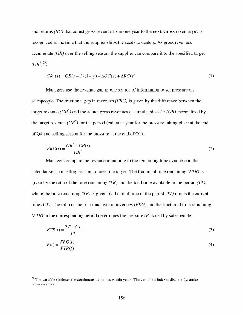
156

and returns (RC) that adjust gross revenue from one year to the next. Gross revenue (R) is

recognized at the time that the supplier ships the seeds to dealers. As gross revenues

accumulate (GR) over the selling season, the supplier can compare it to the specified target

(GR*)29:

)()()1()1()(* sRCsOCgsGRsGR ∆+∆++⋅−= (1)

Managers use the revenue gap as one source of information to set pressure on

salespeople. The fractional gap in revenues (FRG) is given by the difference between the

target revenue (GR*) and the actual gross revenues accumulated so far (GR), normalized by

the target revenue (GR*) for the period (calendar year for the pressure taking place at the end

of Q4 and selling season for the pressure at the end of Q1).

*

* )()(

GRtGRGR

tFRG−= (2)

Managers compare the revenue remaining to the remaining time available in the

calendar year, or selling season, to meet the target. The fractional time remaining (FTR) is

given by the ratio of the time remaining (TR) and the total time available in the period (TT),

where the time remaining (TR) is given by the total time in the period (TT) minus the current

time (CT). The ratio of the fractional gap in revenues (FRG) and the fractional time remaining

(FTR) in the corresponding period determines the pressure (P) faced by salespeople.

TTCTTT

tFTR−=)( (3)

)()(

)(tFTRtFRG

tP = (4)

29 The variable t indexes the continuous dynamics within years. The variable s indexes discrete dynamics between years.

157

3.2. Salespeople’s Effort Allocation

Salespeople allocate their effort between two activities: pushing seeds to or

positioning seeds at dealers. The total effort (TotEff) exerted by a salesperson is assumed

constant at 50 hours a week. The sum of effort to push (EffPush) and position (EffPosit) seeds

result in the total effort, which assumes that salespeople do not shirk. Salespeople respond

promptly and strongly to managerial pressure (P), such as the pressure to meet end-of-year

(gross) revenues target, by pushing seeds to dealers instead of allocating effort to position

seeds. We represent salespeople in aggregation, capturing their mean response over the

distribution of possible response strengths. While individually salespeople differ in the

intensity of their responses, our interviews support that on average they respond similarly to

the same stimuli. For instance, all salespeople interviewed characterized that they faced a

“ crunch time” when trying to meet revenue targets. While all salespeople mentioned that they

expedited dealer orders during crunch time, more experienced salespeople tended to manage

their crunch time more effectively. As one sales team leader confided:

We start out really trying to load toward true grower demand. Everybody makes an honest effort of doing that. But when it gets down to crunch time and teams are looking that they need – say another 10 thousand units to move up a notch on their bonuses – we have to load so much corn that you finally break down and you get to a point where you are just shipping what you can get, where you can get it, and when you can get it. A nonlinear function (f1) captures the impact of pressure on salespeople’ s fractional

allocation of effort to position seeds.

)()()( tPositEfftPushEfftTotEff += (5)

))(()()( 1 tPftTotEfftPositEff ⋅= (6)

0)(,1)0(,0,0 1111 =∞=≤′≥ ffff (7)

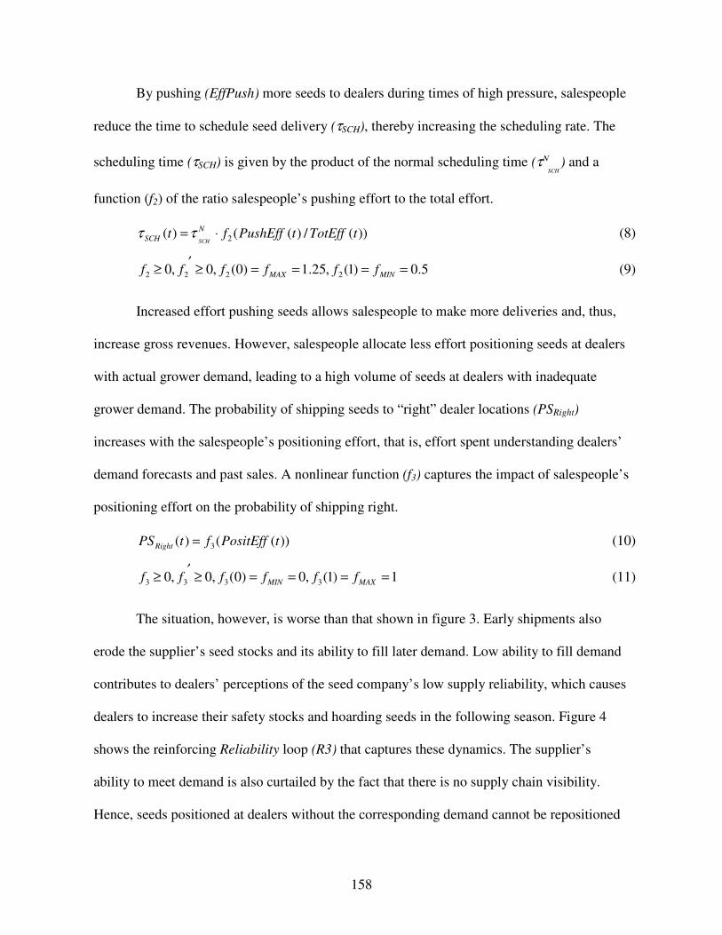
158

By pushing (EffPush) more seeds to dealers during times of high pressure, salespeople

reduce the time to schedule seed delivery (τSCH), thereby increasing the scheduling rate. The

scheduling time (τSCH) is given by the product of the normal scheduling time (τΝSCH

) and a

function (f2) of the ratio salespeople’ s pushing effort to the total effort.

))(/)(()( 2 tTotEfftPushEffft NSCH SCH

⋅=ττ (8)

5.0)1(,25.1)0(,0,0 2222 ====≥′≥ MINMAX ffffff (9)

Increased effort pushing seeds allows salespeople to make more deliveries and, thus,

increase gross revenues. However, salespeople allocate less effort positioning seeds at dealers

with actual grower demand, leading to a high volume of seeds at dealers with inadequate

grower demand. The probability of shipping seeds to “ right” dealer locations (PSRight)

increases with the salespeople’ s positioning effort, that is, effort spent understanding dealers’

demand forecasts and past sales. A nonlinear function (f3) captures the impact of salespeople’ s

positioning effort on the probability of shipping right.

))(()( 3 tPositEffftPSRight = (10)

1)1(,0)0(,0,0 3333 ====≥′≥ MAXMIN ffffff (11)

The situation, however, is worse than that shown in figure 3. Early shipments also

erode the supplier’ s seed stocks and its ability to fill later demand. Low ability to fill demand

contributes to dealers’ perceptions of the seed company’ s low supply reliability, which causes

dealers to increase their safety stocks and hoarding seeds in the following season. Figure 4

shows the reinforcing Reliability loop (R3) that captures these dynamics. The supplier’ s

ability to meet demand is also curtailed by the fact that there is no supply chain visibility.

Hence, seeds positioned at dealers without the corresponding demand cannot be repositioned

159

later. This creates the additional Tied-up Stocks reinforcing loop (R4). In summary, early seed

shipments allow salespeople and the seed supplier to meet the current year’ s revenue target,

but may do so at the expense of the following year’ s performance, as measured in terms of

increased returns, increased salespeople pressure, and low supplier reliability.

Early SeedShipments To

Dealers

Salesforce EffortTo Position Seeds

DealerDemand+

RevenueB1

Revenue

Pressure To MeetRevenue Target

Seeds PositionedAt Wrong Dealers

-

RevenueGoal

RevenueGap

SupplierSeed

Stocks

Supplier’sReliability

SeedsReturned

-

+

Supplier’sAbility To MeetDealer Demand

+

+-

R3

ReliabilityR4

TiedUpStocks

Dealer’sSafetyStocks

+

R1

Returns

-

-

+

-

+

+

GrowerDemand +

-

+

+

R2

SalesforceEffort

Salesforce EffortTo Push Seeds

+Delay

Figure 4. Causal loop diagram mapping supplier reliability and lost sales

The next two sections describe the main assumptions and model formulations for (a)

dealers’ desired orders and (b) supplier production rate generating the dynamics described in

figure 4.

3.3. Dealers’ Desired Orders

Dealers start placing orders with the seed supplier in mid September, two months prior

to the end of the harvest of last years’ crops. When dealers perceive the supplier’ s reliability

160

as low, they place large stock orders to hedge against the possibility of shortages. To estimate

the desired volume of stocked orders (SO*), dealers consider two sources of information:

expected grower demand (GO) and expected return fraction (ERF). When supplier reliability

is high – the supplier can meet dealers’ orders for each hybrid – dealers do not need to

maintain large safety stocks and may order the expected grower demand. The orders will

suffice to meet the demand and there will be few seed returns. When supplier reliability is

low, however, dealers may order more than what they expect to sell to maintain large safety

stocks and meet expected grower demand. As one seed dealer told us:

Usually, we base our orders on last year’ s sales and typically we increase 10-20%/year. We

also order early in the season. By September 15 we can place 50% of stock orders. If it would

be in our benefit to order more than 50% of previous years sales we would do that. For

example, we would order more than that, if we knew that supplies were short. We may learn

this from conversations with our sales rep… Also, if the sales rep would tell me that a certain

variety is on short supply, I would order as much as I could, or as much as my rep would

allow.

Dealers’ perception of the supplier’ s reliability is largely determined by the salient

information provided by seed returns in the previous year. Dealers expect a large fraction of

seed returns in one year if the previous one has also been large. To compensate for the

expected returns, dealers inflate their orders by the amount necessary to adjust for all returns.

The desired volume of stocked orders (SO*) is determined by the ratio of grower demand

(GO) and the complement of the expected returns fraction (ERF). While dealers’ do not have

direct access to expected grower demand, they can get a good estimate of its value by the sum

of total shipments to customers and the growers’ unfilled orders. There may also be similar

hoarding by growers, but for simplicity we assume that dealers know grower demand. In

addition, we assume that grower demand is exogenous.

161

))(1()(*

tERFGO

tSO−

= (12)

The supplier knows that dealers inflate their orders to hedge against shortages, so they

may limit the amount that any dealer can order. The supplier’ s allowed stocked orders (SOA)

set a ceiling to stock orders as a maximum fraction (SOMF), typically 10%, above last years

cumulative sale to growers (CS). The supplier has a good estimate of the volume of sales to

growers by subtracting total shipments to dealers from the seeds returned. For simplicity, we

use cumulative sales in our model.

MFA SOtCStSO ⋅= )()( (13)

3.4. Supplier’s Production Rate

To decide the volume of production the supplier considers two pieces of information:

a term for dealers’ desired stock orders (SO*) and another for inventory adjustment (IA). The

supplier uses a bottoms-up approach for estimating the first term. In particular, the supplier

takes into consideration future sales estimates from sales teams. As noted by a product

manager:

Earlier we used a top-down approach. We decided on a plan and then went out to sell if. Nowadays, we have a bottoms-up approach. We first get input from our sales teams. They give us a sales target for their region. That can be translated into a number of acres that need to be planted, and given the performance of hybrids, into the number of units.

Future sales estimates are based on desired dealer demand (desired stock orders).

Production takes place during the fourth quarter, hence, the ratio of the volume of desired

stock orders (SO*) by the time available for production (τP) determines the first component of

the production rate.

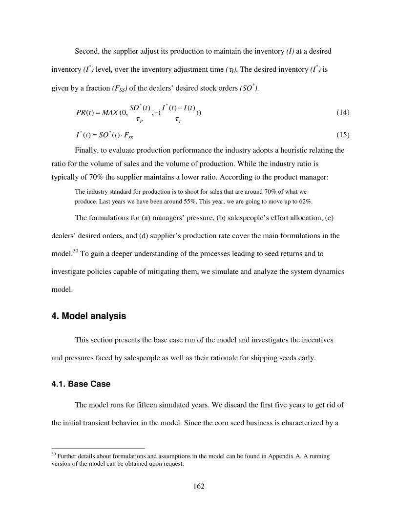
162

Second, the supplier adjust its production to maintain the inventory (I) at a desired

inventory (I*) level, over the inventory adjustment time (τI). The desired inventory (I*) is

given by a fraction (FSS) of the dealers’ desired stock orders (SO*).

)))()(

(,)(

,0()(**

IP

tItItSOMAXtPR

ττ−+= (14)

SSFtSOtI ⋅= )()( ** (15)

Finally, to evaluate production performance the industry adopts a heuristic relating the

ratio for the volume of sales and the volume of production. While the industry ratio is

typically of 70% the supplier maintains a lower ratio. According to the product manager:

The industry standard for production is to shoot for sales that are around 70% of what we produce. Last years we have been around 55%. This year, we are going to move up to 62%.

The formulations for (a) managers’ pressure, (b) salespeople’ s effort allocation, (c)

dealers’ desired orders, and (d) supplier’ s production rate cover the main formulations in the

model.30 To gain a deeper understanding of the processes leading to seed returns and to

investigate policies capable of mitigating them, we simulate and analyze the system dynamics

model.

4. Model analysis

This section presents the base case run of the model and investigates the incentives

and pressures faced by salespeople as well as their rationale for shipping seeds early.

4.1. Base Case

The model runs for fifteen simulated years. We discard the first five years to get rid of

the initial transient behavior in the model. Since the corn seed business is characterized by a

30 Further details about formulations and assumptions in the model can be found in Appendix A. A running version of the model can be obtained upon request.

163

first and fourth quarter business, we assume for simplicity that a simulated year is composed

of 26 simulated weeks accounting for Q1 and Q4. In the beginning of Q4, dealers start placing

their orders with the seed supplier. Several dealers will hoard (stock order) large quantities of

seeds as soon as dealers start accepting orders, in response to the fraction of seeds returned in

the previous year. The remaining orders are placed throughout the selling season, as dealers

gather information on grower orders or as growers place their orders directly with dealers. In

early November, salespeople start scheduling dealers’ orders for delivery. Motivated by the

pressure to meet the supplier’ s revenue targets, salespeople schedule delivery before the end

of the calendar year. Figure 5a shows the ordering and scheduling rates. Shipments to dealers

(Figure 5b) start in mid November (week 20), increasing sharply due to these financial

pressures.

Orders600,000

300,000

0

0 26 52 78 104 130Time (Week)

Scheduling Rate

Order Rate

Units

/ W

eek

Orders600,000

300,000

0

0 26 52 78 104 130Time (Week)

Scheduling Rate

Order Rate

Units

/ W

eek

Shipments500,000

250,000

00 26 52 78 104 130

Time (Week)

Shipments500,000

250,000

00 26 52 78 104 130

Time (Week)

Figure 5. (a) Inflow and outflow of dealer orders and (b) supplier shipments

The supplier sets a revenue goal based on last year’ s revenues adjusted for the

additional costs of returns and obsolescence. The supplier recognizes sales revenue at the time

the seeds are shipped to dealers. Corn seed prices ($100/bag), return costs ($20/bag), and

obsolescence costs ($5/bag) are constant throughout the simulation. Initially in the quarter,

pressure to meet the revenue target is low since salespeople have plenty of time to make sales.

164

This pressure on salespeople (Figure 6a) increases, however, as time goes by and the end of

the quarter approaches. The graph has a peak at the end of Q4, indicating an increase in

pressure due to the little time availability to meet the revenue targets for the fiscal year ending

in December. During high-pressure “ crunch” periods, salespeople allocate most of their effort

(time) pushing seeds to dealers and almost no effort positioning them adequately. Figure 6b

shows salespeople’ s efforts in pushing and positioning seeds.

Pressure on Salespeople4

2

00 26 52 78 104 130

Time (Week)

Pressure on Salespeople4

2

00 26 52 78 104 130

Time (Week)

Salespeople’s Effort 1

0.5

00 26 52 78 104 130

Time (Week)

Push EffortPosition

Effort

Salespeople’s Effort 1

0.5

00 26 52 78 104 130

Time (Week)

Push EffortPosition

Effort

Figure 6. Salespeople (a) pressure to meet goals and (b) effort to position/push seeds

As pressured sales people push seeds, they incur a greater probability of sending it to

dealers where no corresponding grower demand is available. Figure 7a shows that the

probability of sending seeds to the “ right” locations decreases as the pressure on salespeople

increases with the end of the year. This leads to a stock of seeds in “ wrong” locations – where

no grower demand is available (figure 7b) – that will ultimately return to the seed supplier.

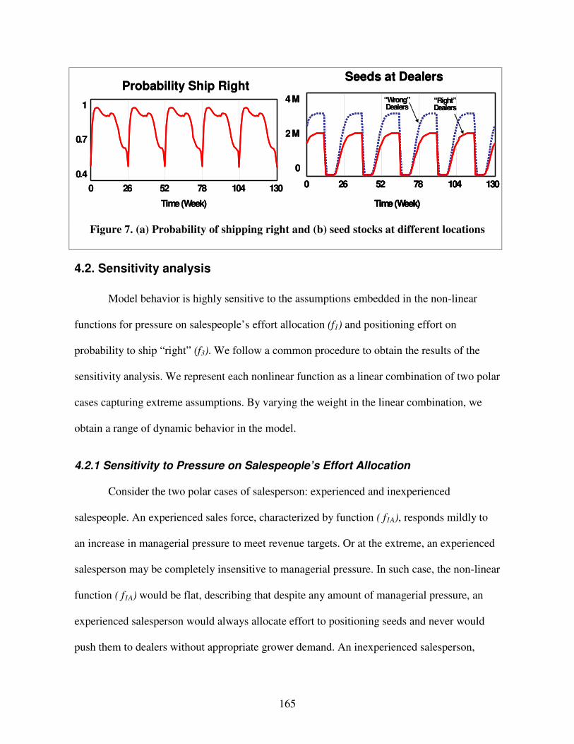
165

Probability Ship Right1

0.7

0.40 26 52 78 104 130

Time (Week)

Probability Ship Right1

0.7

0.40 26 52 78 104 130

Time (Week)

Seeds at Dealers

4 M

2 M

0

0 26 52 78 104 130

Time (Week)

“Right”Dealers

“Wrong”Dealers

Seeds at Dealers

4 M

2 M

0

0 26 52 78 104 130

Time (Week)

Seeds at Dealers

4 M

2 M

0

0 26 52 78 104 130

Time (Week)

“Right”Dealers

“Wrong”Dealers

Figure 7. (a) Probability of shipping right and (b) seed stocks at different locations

4.2. Sensitivity analysis

Model behavior is highly sensitive to the assumptions embedded in the non-linear

functions for pressure on salespeople’ s effort allocation (f1) and positioning effort on

probability to ship “ right” (f3). We follow a common procedure to obtain the results of the

sensitivity analysis. We represent each nonlinear function as a linear combination of two polar

cases capturing extreme assumptions. By varying the weight in the linear combination, we

obtain a range of dynamic behavior in the model.

4.2.1 Sensitivity to Pressure on Salespeople’s Effort Allocation

Consider the two polar cases of salesperson: experienced and inexperienced

salespeople. An experienced sales force, characterized by function ( f1A), responds mildly to

an increase in managerial pressure to meet revenue targets. Or at the extreme, an experienced

salesperson may be completely insensitive to managerial pressure. In such case, the non-linear

function ( f1A) would be flat, describing that despite any amount of managerial pressure, an

experienced salesperson would always allocate effort to positioning seeds and never would

push them to dealers without appropriate grower demand. An inexperienced salesperson,

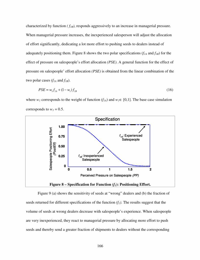
166

characterized by function ( f1B), responds aggressively to an increase in managerial pressure.

When managerial pressure increases, the inexperienced salesperson will adjust the allocation

of effort significantly, dedicating a lot more effort to pushing seeds to dealers instead of

adequately positioning them. Figure 8 shows the two polar specifications (f1A and f1B) for the

effect of pressure on salespeople’ s effort allocation (PSE). A general function for the effect of

pressure on salespeople’ effort allocation (PSE) is obtained from the linear combination of the

two polar cases (f1A and f1B).

1B1A fwfwPSE )1( 11 −+= (16)

where w1 corresponds to the weight of function (f1A) and w1∈ [0,1]. The base case simulation

corresponds to w1 = 0.5.

Specification

Perceived Pressure on Salespeople (PP)

f1A: Experienced Salespeople

f1B: Inexperienced Salespeople

1.00

0.75

0.50

0.25

00 0.5 1 1.5 2S

ales

peop

le P

ositi

onin

g E

ffort

(Pos

itEff)

Specification

Perceived Pressure on Salespeople (PP)

f1A: Experienced Salespeople

f1B: Inexperienced Salespeople

1.00

0.75

0.50

0.25

00 0.5 1 1.5 2S

ales

peop

le P

ositi

onin

g E

ffort

(Pos

itEff)

Figure 8 – Specification for Function (f1): Positioning Effort.

Figure 9 (a) shows the sensitivity of seeds at “ wrong” dealers and (b) the fraction of

seeds returned for different specifications of the function (f1). The results suggest that the

volume of seeds at wrong dealers decrease with salespeople’ s experience. When salespeople

are very inexperienced, they react to managerial pressure by allocating more effort to push

seeds and thereby send a greater fraction of shipments to dealers without the corresponding

167

grower demand. When salespeople are experienced, they do not respond to managerial

pressure. An experienced salesperson “ breaks” the feedback response from actual revenues to

effort to position seeds, avoiding the problem of shipping seeds to the wrong dealers.

Seeds at Wrong Dealers

Time (Week)

3 M

1.5 M

0

0 26 52 78 104 130

100% Ex

75% Ex

50% Ex25% Ex0% Ex


Time (Week)

3 M

1.5 M

0

0 26 52 78 104 130

100% Ex

75% Ex

50% Ex25% Ex0% Ex

Fraction of Seeds Returned

Time (Week)

1.00

0.50

00 26 52 78 104 130

100% Ex

75% Ex

50% Ex25% Ex

0% Ex


Time (Week)

1.00

0.50

00 26 52 78 104 130

100% Ex

75% Ex

50% Ex25% Ex

0% Ex

Figure 9 – Sensitivity of seeds at “wrong” dealers and returns to salespeople’s responses.

4.2.1 Sensitivity to Position Effort on Probability

Consider the two extreme cases of the quality of dealers’ orders. High quality orders,

described by function (f3A), are characterized by a perfect correlation between dealer and

grower orders, reflecting the case of perfect orders. When dealer orders perfectly reflect actual

grower demand, a lack of salespeople’ s effort causes no impact on the adequate positioning of

seeds. Even if inexperienced salespeople pushed sales to dealers, by speeding delivery of

previously placed orders, seeds would still be sent to the “ right” dealers. On the other hand,

low quality orders, described by function (f3B), are characterized by a poor correlation

between dealer and grower demand. Imperfect dealer orders suggest that a lack of

salespeople’ s effort on positioning seeds can lead to a large fraction of seeds at “ wrong”

dealers. Figure 10 shows the two polar specifications (f3A and f3B) for the probability of

168

shipping right (PPR). A general function for the effect of positioning effort on the probability

to send to “ right” dealers (PPR) is obtained from the linear combination of the two polar cases

(f3A and f3B).

3B3A fwfwPPR )1( 22 −+= (17)

where w2 corresponds to the weight of function (f3A) and w2∈ [0,1]. The base case simulation

corresponds to w2 = 0.5.

Specification

Perceived Effort to Position Seeds (PPositEff)

f3A: High Quality Orders

f3B: Low Quality Orders

1.00

0.75

0.50

0.25

00 0.25 0.5 0.75 1

Pro

babi

lity

Shi

ppin

g R

ight

(P

SR

ight)

Specification

Perceived Effort to Position Seeds (PPositEff)

f3A: High Quality Orders

f3B: Low Quality Orders

1.00

0.75

0.50

0.25

00 0.25 0.5 0.75 1

Pro

babi

lity

Shi

ppin

g R

ight

(P

SR

ight)

Figure 10 – Specification for Function (f3): Probability of Shipping to Right Dealers.

Figure 11 (a) shows the sensitivity of seeds at “ wrong” dealers and (b) the fraction of

seeds returned for different specifications of the function (f3). The results suggest that the

volume of corn-seeds at wrong dealers decrease with the quality of dealers’ orders. When

orders have a poor correlation with grower’ s orders, there is a high probability that corn seeds

will end up at dealers without the corresponding grower demand. When the quality of dealer’ s

orders is high, it can “ break” the feedback influence of salespeople’ s effort to position seeds

to the probability of shipping to right dealers, which avoids the problem of shipping seeds to

the wrong dealers.

169

5 M

2.5 M

00 26 52 78 104 130


100% Qua75%

Qua50% Qua25%

Qua

0% Qua

Time (Week)

5 M

2.5 M

00 26 52 78 104 130


100% Qua75%

Qua50% Qua25%

Qua

0% Qua

Time (Week)


Time (Week)

1.00

0.50

00 26 52 78 104 130

100% Qua

75% Qua

50% Qua

25% Qua

0% Qua


Time (Week)

1.00

0.50

00 26 52 78 104 130

100% Qua

75% Qua

50% Qua

25% Qua

0% Qua

Figure 11 – Sensitivity of seeds at wrong dealers and returns to data quality.

The base case simulation shows how pressure to meet the revenue target can lead to

poor allocation of effort by salespeople, resulting in an increase in seed returns. The next

section explores the incentives faced by salespeople and the intended rationality of their

actions.

4.3. The case for sending seeds early

While emphasis on pushing seeds may not seem rational in the long-term, sales people

have huge incentives to do this. First, salespeople’ s financial rewards are directly proportional

to meeting revenue targets. Bonuses, ranging from zero to 40% of base salary, depend on the

fraction of the revenue quota the team achieves. Not meeting the quota has a clear negative

impact: the team receives a low bonus. There is no ambiguity in the costs associated with such

outcomes. This is in sharp contrast with the costs associated with returns. Sales teams are

charged an “ obsolescence rate” for returned seeds that spoil. All teams, regardless of

individual contribution to total returns, share equally these costs. The salespeople we

interviewed were unable to specify the policy used to charge them for obsolescence costs.

170

More importantly, they could not quantify the dollar value that the charge represented.

Furthermore, salespeople are charged for the direct costs associated with sales not made

(returns). While salespeople do not experience a direct reduction in their bonuses as a result of

returns, their revenue targets for the following year are adjusted upwards to account for any

lost revenue. While there are clear and unambiguous monetary benefits to pushing seeds to

dealers, the costs are ambiguous and translate into higher revenue targets instead of a

monetary disincentive.

Second, the rewards accrued for pushing seeds occur closer in time to salespeople’ s

actions. Salespeople receive their bonuses at the end of the calendar year (Q4), just as pushing

seeds to dealers has peaked. Hence, salespeople have very salient information about the

strength of their actions and the resulting outcome. In sharp contrast, seed returns take place at

the end of the selling season (end of Q1) in the following calendar year, at which time the

associated costs are taken into consideration. The costs associated with each sales team’ s

returns lead to higher revenue targets in the following year. In summary, the costs associated

with pushing seeds accrue one year after the benefits. Hence, the incentives to pushing seeds

to dealers are not only unambiguous but they take place shortly after the actions are made.

Third, it takes much less effort to push seeds than to position them. Consider the

amount of time and effort associated with positioning the seeds in dealers with adequate

demand. The salesperson must first call the dealer to schedule a personal visit, where both can

go over the current replenishment plan. Prior to the visit, dealers can explore potential grower

demand and salespeople retrieve last year’ s sales information for their reference. At the

scheduled date, the sales representative visits the dealer to discuss future ordering plans,

which can take a whole day or at least one afternoon. Now consider the time and effort

171

required to push seeds to dealers. In some cases, this boils down to a telephone call of a few

minutes where the sales representative lets the dealer knows that he is sending some bags of

seeds earlier than expected to meet the sales goals. Most dealers have already placed a large

number of orders with the supplier, which they expect to receive some time during the season,

so most of the salesperson negotiation focuses on early delivery. Laid-back salespeople are

clearly better-off (in the short-term) by pushing seeds to dealers instead of trying to position

them. Even industrious salespeople will be tempted to shift to pushing seeds when pressured

to meet revenue targets. The uneven amount of effort to push and position seeds is likely to

lead pressured salespeople to choose the former instead of the latter.

Finally, the early timing of benefits compared to costs generates an important

reinforcing loop that intensifies the detrimental dynamics leading to high returns. When

salespeople push sales to ease the short-term financial pressure, they generate returns in the

following year. The supplier then adds the costs of returns to the following year revenue

targets of the corresponding salespeople. Hence, in the following season, salespeople must

meet an even higher revenue target and endure even more pressure than the previous year.

Under additional stress, they are likely to rely even more on the pushing seeds strategy, which

will lead to even higher returns in the following year. When salespeople enter into the mode

of pushing seeds to meet revenue targets, the reinforcing loop makes it very difficult for them

to change the situation.

5. Policy Analysis

Next, we explore policies that can mitigate the costs of high seed returns. We analyze

four types of policies. The first policy – Order pacing policy – limits the initial pace of

dealers’ orders. The second policy – Fiscal year policy – shifts the fiscal year from the

172

calendar year to the selling season year. The third policy – Salespeople’ s playbook policy –

provides salespeople with a framework that helps them take action in the face of pressure.

And the fourth policy – Early ship policy – provides salespeople additional time to meet their

revenue target.

5.1. Order Pacing Policy

This policy establishes a pace for dealers’ ordering rate. First, it limits dealer’ s initial

volume of stock orders, establishing a maximum stock order of 50% of previous year’ s sales

(net of returns) that can be placed when the supplier starts accepting orders. Then, it imposes

a maximum pace for subsequent orders, i.e., dealers can place the remainder of their orders

uniformly throughout Q4, reaching 75% in mid October, and 100% in mid November. Since

the remaining stock orders are delayed, we allow them to have better quality. While dealers

placed most of their orders before grower demand information becomes available – growers

do not place most of their orders until late November or December (Figure 3) – dealers’ fears

of scarcity of desired seed hybrids motivated them to place large orders early in the season.

For instance, if dealers sold 500 bags of a specific hot hybrid in the previous year, they would

not hesitate in placing an order for more than 250 bags in mid September. This pattern of

order pacing reflects a policy actually implemented by the seed supplier. Prior to this policy,

dealers’ placed large stock orders in the beginning of Q4, leaving many regions (and dealers)

without any supply. Figure 12 shows the stock of seeds at wrong dealers for this policy

compared to the base case. The order pacing policy reduces returns by 12%. This policy was

successfully implemented by the seed supplier, allowing them to improve supply of high

performing across all dealers.

173

5.2. Fiscal year policy

This policy shifts the fiscal year for the company allowing it to shift the pressure on

salespeople from the end of the calendar year (end of Q4) to the end of the selling season (end

of Q1). This policy has two direct benefits in reducing the volume of returns. First, it allows a

much longer amount of time for salespeople to meet their revenue targets. Reducing the

pressure experienced by salespeople will avoid the need to push seeds to dealers, and

substantially reduce the volume of seeds returned. Second, by closing the books at the end of

selling season, the supplier can postpone the starting date to receive dealer’ s orders. This

allows dealers more time to gather grower demand information and place orders that more

closely reflect them. We introduce this policy by shifting the end date of the annual period to

meet the revenue target. Figure 12 (a) shows the inventory at wrong dealers for this policy;

Figure 12 (b) shows the fraction of returns. The fiscal year policy reduces returns by 56%.

This policy yields a large impact because it addresses the main cause of returns: the

managerial pressure to meet financial targets. The supplier considered implementing this

policy, but that has not yet taken place.

5.3. Salespeople’s playbook policy

Salespeople have a dual role of pushing and positioning seeds. This policy emphasizes

the important role played by sales teams in positioning seeds. Its intention focuses on

minimizing the impacts of pressure on salespeople’ s behavior. Our interviews suggest that

while salespeople respond to financial pressure in a similar way, inexperienced sales people

were more prone to pushing seeds to the wrong dealers. Their lack of experience results in

inadequate planning and postponed contacts with dealers. One sales team leader explained

one way he managed his seed portfolio:

174

I have my agronomist go through and analyze our entire portfolio and say what are the four or five key hybrids or varieties that we are going to hand our head on in [the following year]. I don’ t want fourteen million products that we are going to sell out here. We can’ t be all things to all people out there. We’ ve got to focus on the four or five that we know that will perform well for our growers out there and make them more money than the competition. Yet, we are going to have other SKUs besides that, but we are going to focus on the four or five. In addition, the interviews suggest that inexperienced salespeople respond more

aggressively to financial pressure, resorting more frequently and more strongly to pushing

seeds to dealers. This policy suggests the implementation of a protocol, or playbook, capable

of supporting salespeople’ s desired behavior. We implement this policy in the model by

introducing a function for sales people response that has a smaller slope to the pressure input.

Figure 12 (a) shows the seed stocks at wrong dealers and Figure 12 (b) shows the fraction of

returns for the salespeople’ s playbook policy. This policy reduces returns by 39%. The seed

supplier has been emphasizing grower order accuracy, but we believe that there are still other

opportunities to improve focus for sales teams. For example, one sales team leader shared the

strategy used to get salespeople’ s focus:

We had a little business card that had corn hybrids on one side and soybeans on the other, and it said what percent of the total mix we had of [a specific] product. So, [hybrid X], for example, was 18% of our total [team] supply. Everybody [in our team] knew what the top 10 hybrid varieties were. Everybody knew what we needed to be promoting. Everybody knew what we needed to be selling. Everybody knew what we needed to be positioning at a dealer. So, once you get that kind of knowledge and you go through that intensive process you are going to do a lot better job managing your supply in October, November, and December. The playbook policy suggests that there are opportunities for making wide spread use

of techniques developed by the existing salespeople, so that teams can learn from each others

best practices.

175

5.4. Early ship policy

In this policy, the supplier anticipates the starting shipment date to dealers. This policy

provides salespeople with additional time to meet their revenue targets, reducing the financial

pressure they experience. Under lower stress levels, salespeople have an opportunity to

position more seeds, correcting some of the discrepancies introduced during the early stock

ordering process. This policy increases the probability that seeds are sent to the right dealers,

which in turn reduces the amount of seeds returned. We implement this policy by allowing the

seed company to start scheduling delivery of seeds two weeks in advance (early November).

Since shipping early does not change the timing that dealers are placing their orders, it does

not have any impact on the probability of shipping to adequate locations. Figure 12 (a) shows

the stock of seeds at wrong dealers and Figure 12 (b) the fraction of returns for this policy

compared to the base case and other policies. The early ship policy reduces returns by 4%.

Seeds at Wrong Dealers2 M

1 M

00 26 52 78 104 130

Time (Week)

EarlyShip

Base Order Pace

Fiscal Year

Playbook


1 M

00 26 52 78 104 130

Time (Week)


1 M

00 26 52 78 104 130

Time (Week)

EarlyShip

Base Order Pace

Fiscal Year

Playbook

Fraction of Returns0.6

0.5

0.4

0.3

0.20 26 52 78 104 130

Time (Week)

EarlyShipBase

Order Pace

Fiscal Year

Playbook

Fraction of Returns0.6

0.5

0.4

0.3

0.20 26 52 78 104 130

Time (Week)

EarlyShipBase

Order Pace

Fiscal Year

Playbook

Figure 12. (a) Seeds at wrong dealers and (b) fraction of returns for different policies.

Table 1 presents a summary of the results for all policies investigated. The supplier

can effectively reduce returns (by 39% or more) by emphasizing measures that reduce the

pressure experienced by salespeople and promote a conservative response to financial

pressure. Two policies (salespeople’ s playbook and fiscal year) reduce returns addressing the

effect of financial pressure on salespeople. The first policy provides salespeople with a best

176

practice protocol that helps then to meet dealer demand without heavily depending on pushing

seeds. The second policy shifts the pressure to the end of the selling season, giving

salespeople plenty of time to meet the financial pressure. The policies reduce returns by 39%

and 56%, respectively.

Table 1. Summary results for policy analysis addressing reduction in seed returns.

Policy Net Revenues (Million $ /

year)

Revenue Improvement

(%)

Returns (Million $ /

year)

Return Improvement

(%) Base 254 – 38.7 – Order Pace 273 7.5 33.9 12 Fiscal Year 288 13.4 17.1 56 Playbook 269 5.9 23.6 39 Early Ship 254 0 37.2 4

6. Discussion

Seed hoarding and returns result from the interplay between human behavior (e.g.

salespeople’ s effort allocation decisions, dealers’ ordering decisions, supplier’ s production

heuristics, and managers’ pressure) and supply chain characteristics (e.g. fixed product mix,

timing of information availability, and quality of dealers’ orders). While system dynamics has

a long tradition of investigating the interplay of human decision making in different

industries, this research provides an application to the agribusiness industry and provides

insight into the mechanisms that lead to seed hoarding.

Although the intrinsic characteristics of corn-seed production, making available a

fixed mix of products, influence dealers’ hoarding behavior, a number of actions by the

supplier can intensify dealers’ inflationary behavior. For instance, a number of unintended

consequences are triggered by the intendedly rational decision rules of managers and

salespeople. To ease the managerial pressure to meet gross annual revenue targets,

177

salespeople push seeds to dealers. Early shipments allows salespeople to meet the financial

goals, however, the hybrids may end up at dealers lacking the appropriate grower demand.

While managerial pressure has the desired consequence of increasing gross revenues and

meeting financial goals, it also closes a number of positive loops that work in a detrimental

way. Early seed shipments lead to poor positioning of hybrids with dealers. Ultimately, the

hybrids end up in locations with inadequate grower demand, resulting in an increase in corn-

seed returns, and further increase in financial pressure in the following year. Hence, the

positive Returns (R1) loop leads to a higher fraction of seed returns this year and an even

greater managerial pressure in the following year. In addition, the financial pressure to meet

gross annual revenue targets creates strong disincentives for salespeople to position seeds.

The limited effort devoted to positioning seeds increases the probability of sending them to

dealers without corresponding grower demand. This positive Sales-force Effort (R2) loop will

increment the volume of seed returns this year and the financial pressure in the following

year.

The positive loops above, motivated by salespeople’ s responses to financial pressure,

drive the system to a mode of operation characterized by high returns and financial pressure.

These conditions further interact with the supplier’ s production heuristic creating an

additional positive loop that intensifies the problem. As the volume of returns increase, the

supplier increases the volume of production to maintain a desired level of inventory and sales.

With larger inventories, the supplier can meet a greater fraction of dealers’ orders, leading to

more shipments and, everything else equal, more returns. The reinforcing “ supplier

production” loop also contributes to an increase in returns and financial pressure. The

problem is intensified even more by dealers’ ordering heuristics. Dealers’ desired stock orders

178

increase with the volume of returns. Higher orders lead to more shipments and, everything

else equal, higher returns. The positive Reliability (R3) loop contributes even more to a high

volume of returns and increased financial pressure. Hence, dealers’ hoarding behavior is

largely intensified by the suppliers’ heuristics. While salespeople’ s effort to push seeds to

dealers may be effective in reducing the short-term financial pressure, they can lead to a long-

term increase in returns and financial pressure.

This research suggests a number of initiatives that can help the supplier reduce seed

returns. First, the seed supplier can control the pace of dealers’ orders. Currently, dealers can

stock-up all of previous years’ sales as soon as the supplier starts accepting orders. Dealers’

over-ordering of specific seed hybrids can deprive entire regions of such hybrids, creating

further incentives for all dealers to over-order in the following season. By controlling the pace

of dealers’ orders the supplier can ration the hybrids among all its dealers, allowing seeds to

reach the dealers that are not over-ordering and also reducing dealers’ need to over-order in

the following season. While rationing does provide some dealers with an incentive to

intensify over-ordering, it is less effective when the supplier controls the number of orders

allowed. Second, the supplier can shift the fiscal year to coincide with the end of the selling

season. This policy allows the supplier to meet their financial goals for the fiscal year in the

end of the selling season (Q1) instead of the end of the calendar year (Q4). Changing the

fiscal year shifts the pressure experienced by salespeople to the end of Q1, providing them

with significantly more time to meet their targets. This policy further allows dealers to gather

more reliable information about true grower demand, minimizing the need for dealer over-

ordering. Third, the supplier can provide a “ playbook” to guide salespeople’ s behavior. Since

salespeople face tremendous pressure to meet financial goals, it is not surprising that they may

179

focus their attention on pushing seeds instead of positioning them. While the supplier

emphasizes the importance of salespeople’ s role in positioning seeds, we suggest a more

practical approach. For example, the supplier could suggest the specific five hybrids that

salespeople should focus on. In addition, the “ playbook” could map challenges and contingent

plans throughout the selling season to guide salespeople’ s actions and provide mechanisms to

effectively prevent salespeople from giving into the pressure to meet the revenue targets.

Fourth, the supplier can anticipate the initial date to start shipping seeds to dealers, to provide

salespeople with more time to meet revenue targets. Easing part of the financial pressure

faced by salespeople may allow them to emphasize on grower order accuracy. Our results

suggest, however, that this policy may have a limited impact on behavior. Our analysis

underscores the important role of salespeople’ s responses in the issue of seed returns. Overall,

these policies stress the importance of grower order accuracy, particularly through the

information gathered by salespeople as a proxy for actual grower demand. As one sales team

leader told us: “ [What we need are] real orders for real people.” Relying on dealers’ inflated

stocked orders as a basis for shipments to dealers may simply not allow the supplier to reduce

the amount of returns.

The results raise a number of issues regarding implementation. First, a salespeople

“ playbook” allows the rapid implementation of a policy that influences salespeople’ s

responses. While hiring experienced people and diligent training would be a desirable

alternative, it may take several years before the supplier can reap its benefits. An effective

policy in the short-term may focus on developing a “ best practice sales workshop”

championed by experienced sales people. Such workshop would provide guidelines for

actions and conduct to salespeople. The resulting framework could have a timeline for actions

180

and achievements during the selling season. The guidelines could also provide a set of

contingencies (questions to illuminate the potential causes of the problems and possible

contingent actions) to guide salespeople’ s responses, when they face difficulty in keeping up

with the timeline. A set of well established guidelines for salespeople’ s responses could allow

them to behave more like experienced salespeople.

In addition, managers recognize that allowing returns in the first place is part of the

problem. This practice, however, is industry standard. Managers hold the strong belief that

more stringent return policies can lead to loss of market share. A potential solution that

managers considered to tackle the excess returns was to rely directly on grower order demand.

The ability to compare dealers’ orders directly with grower’ s orders would allow the seed

company to realize which dealers were hoarding which seed hybrids. Implementing such a

policy, however, faced several constraints, such as getting the data on grower’ s orders and

using it effectively. In terms of the former, many dealers are unwilling to share grower orders

with the seed supplier. They fear that the company might use the data to bypass them and sell

directly to growers. In terms of the latter, managers claimed that even if they could obtain the

data on grower orders, they might not have use for it. Since grower orders become available

only in late November, waiting for such data would not allow the company to meet its annual

revenue quota. In addition, the supplier relies on the storage capacity of local dealers to stock

the volume of seeds produced within the season.

While order pacing limited the volume of early orders and constrained dealers’

hoarding behavior, some managers contended that the policy was a mixed blessing. On one

hand, the supplier benefited from reduced hoarding of hot selling hybrids. On the other hand,

it also reduced orders for other products. For instance, by waiting a couple of months before

181

placing all its orders, dealers were able to avoid ordering products that were perceived to not

perform so well, reducing the supplier’ s ability to sell products that were less appealing to

dealers. Naturally, this argument fails to account for the fact that some of the seeds ordered by

mistake would potentially be returned anyway, resulting in even higher costs (due to

transportation, retesting and re-bagging.) Managers that were against the order pacing policy

claimed that returns were an intrinsic part of the business and they were willing to accept

some level of returns. As one manager put it:

Unfortunately, in the seed business my perception is that it is almost a little bit of the nature of the beast. You are going to have returns. There is no 100% here. You can certainly work to minimize returns, and I think what we’ re trying to do as a company is to [ask] what is an acceptable amount of returns? Right now, we see that we are in excess of that and so we’ d like to lower those returns from what they are today. But this is not a zero-sum game. You are not going to get them all of the way down to zero. It’ s the nature of the beast. When you are dealing with an industry influenced by the environment, orders change with time, they change by the day. This work raises a number of possibilities for future research. A promising possibility

is to study how hybrids of different performance can impact the results presented here. It was

clear from our interviews that it is important for the supplier to emphasize the management of

the whole product portfolio. Frequently, high performing seeds are quickly allocated to some

dealers, when compared to low performing ones, often leaving other dealers with a perception

that supply (for the products they want) is unreliable. In turn, perceived supplier unreliability

potentially leads to seed hoarding in the following season. Furthermore, focus on high

performing seeds leaves the supplier with unallocated low performing seeds, increasing the

ratio of production to sales, augmenting costs, and decreasing supplier performance. Hence,

the supplier must emphasize management of high performing hybrids, allocating them

carefully across dealers, to avoid hoarding and to manage dealer’ s perceptions about supply

availability and supplier reliability. For instance, the supplier can inform dealers about the

182

adopted allocation policy for “ hot” products and provide frequent updates on their

availability. When high performing hybrids run out, the supplier may shift dealers’ attention

to other recommended hybrids. For instance, the supplier can suggest hybrids are good

substitutes for specific “ hot” products. In this context, it would be interesting to investigate

the effectiveness of the previous policies when we model explicitly seed performance and

account for dealers’ preferences towards high performing seeds.

Finally, there is an opportunity to explore how other financial incentives can shape

salespeople’ s and dealers’ responses. In particular, the obsolescence charge used by the

supplier is equally distributed among all salespeople. This creates an incentive for salespeople

to push seeds, leading to potentially higher returns. By pushing additional seeds, salespeople

get the full benefits of additional sales, but avoid some of the associated costs, since other

salespeople pay for a fraction of the obsolescence costs. Subsequent to our intervention the

policy was adjusted to proportionately impact sales teams based on their contribution to

obsolescence. While this is a step in the right direction, other opportunities remain for

creating the right incentives for dealers and salespeople. For instance, the lack of adequate

incentives to dealers also contributes to the volume of seed returns. Dealers face significant

penalties for under-stocking corn-seeds, including sales and reputation losses. There are few

or no penalties for over-stocking seeds, however. Prior to the 2000 season, dealers could send

hybrids back to the seed manufacturer without any penalties. When seed returns rose in excess

of 25% the supplier introduced an incentive plan charging dealers a restocking fee of 2% of

the tag price, for seeds returned after February 28 – nearly at the end of the selling season –

and in excess of the industry average. Even with this mild incentive – allowing dealers a

significant amount of time to assess grower demand and no charges for returns within 15% –

183

returns decreased the following season, perhaps because some dealers reduced their hoarding.

This policy has suffered strong opposition and at one point was almost removed due to

increased resistance from dealers and some managers at the seed supplier. Despite the

resistance, the supplier adopted an additional incentive scheme in the last season. A product

manager explains:

We are keeping the old incentive policy that charges $2 per unit (bag) returned and adding a new incentive policy. The new policy adds a charge to the dealers’ compensation package. Usually, we sell corn seeds for $100 and give back $11 to dealers as an incentive. When returns are over 20%, dealers loose 2% of total compensation. So for a bag of corn that may be sold for $100, the margin to the dealer is often around $10. A 2% charge of total compensation is $2, or 20% of their margins. So, this is a significant incentive. In parallel with the implementation of punishment mechanisms for actions that lead to

returns, the supplier can also implement policies that reward sales teams, dealers, and growers

for low seed returns. Our interviews suggest that many dealers are successful in providing

incentives for customers to place orders early. Finally, for both types of incentives it is crucial

that the seed supplier provide complete visibility of the costs and rewards of different

incentive systems, if it hopes them to be successful.

7. References

Anonymous. 1974. The New York Times, February 15, Friday, Page 14, Column 5.

Donohue, K. 1996. “ Supply Contracts for Fashion Goods: Optimizing Channel Profits.” Working Paper, The Wharton School, Philadelphia, PA.

Emmons, H. and S. Gilbert. 1998. “ Note. The Role of Returns Policies in Pricing and Inventory Decisions for Catalogue Goods.” Management Science. 44(2): p. 276-283.

Forrester, J.W. 1968. “ Market Growth as Influenced by Capital Investment.” Industrial Management Review. 9(2): p. 83-105.

Gonçalves, P. 2002. “ When do minor shortages inflate to great bubbles?” Proceedings of the2002 International System Dynamics Conference. System Dynamics Society: Albany, NY.

184

Shi, S. 2002. “ Phantom Orders Roil Cisco’ s Supply Chain–A System Dynamics Study of Networking Equipment Industry’ s Supply Chain.” Unpublished master’ s thesis, MIT, Cambridge, MA.

Jones, P.; T. Lowe; R. Traub; G. Kegler. 2002. “ Matching Supply and Demand: The Value of a Second Chance in Producing Hybrid Seed Corn.” Manufacturing and Service Operations Management. 3(2): p.122-137.

Jones, P.; G. Kegler; T. Lowe; R. Traub. 2003. “ Managing the Seed-Corn Supply Chain at Syngenta.” Interfaces. 33(1): p.80-90.

Merton, R. K. 1948. The self-fulfilling prophecy. Antioch Review. 8: p.193-210.

Padmanabhan, V. and I.P.L. Png. 1995. “ Returns Policies: Make Money by Making Good.” Sloan Management Review. Fall. p. 65-72.

Padmanabhan, V. and I.P.L. Png. 1997. “ Manufacturer’ s Returns Policies and Retail Competition.” Marketing Science. 16 p. 81-94.

Petersen, M. 2002. “ Anthrax and Anxiety.” The New York Times, March 10, Sunday, Section 3, p. 4. Column 5.

Richardson, G. and A. Pugh. 1980. Introduction to System Dynamics Modeling with Dynamo. Productivity Press, Portland, Oregon.

Sterman, J.D. 1989a. Modeling Managerial Behavior: Misperceptions of Feedback in a Dynamic Decision Making Experiment. Management Science. 35(3): p. 321-339.


Webster, S. and Z. Weng. 2000. “ A Risk-free Perishable Item Returns Policy.” Manufacturing and Service Operations Management. 2(1): p. 100-106.

Weiss, J. 1999. The Boston Globe, December 31, Friday, p. B1.

185

Appendix A: Model description

The purpose of the modeling effort is to explore the causes of seed returns and derive

policies capable of reducing them. The model captures dealers’ ordering decisions,

salespeople’ s effort allocation decisions, and managers’ incentives at the seed supplier to meet

sales targets. These actions contribute directly to seed hoarding, which results in returns. The

paper explores the effect that financial pressure to meet the annual sales targets has on

salespeople’ s effort allocation, resulting in pushing shipments of corn seeds to dealers and

failing to position them adequately. The combination of early seed shipments and inadequate

positioning at dealers influences the volume of seed returns.

In alignment with the model purpose, we adopt a level of aggregation that is

sufficiently high to focus on the interaction of the seed supplier with its dealers through the

company’ s sales force. Hence, we avoid detail complexity (e.g., multiple supplier warehouses,

multiple dealer locations, and multiple products) that does not directly contribute to the

dynamics of interest. Our model considers a supplier producing a single corn-hybrid and

aggregates all corn-seed inventory in a single warehouse. While seed hybrids have different

performance, both high and low performing products suffer from returns, due to dealers’

attempts to hoard products early in the season and their inability to foresee which hybrids will

become high or low performing products. Instead of investigating low and high performing

products, we build a generic model and change parameters (e.g., the effect of positioning on

shipping) when dealing with different types of hybrids. Here, we focus on high performing

products.

A few months prior to harvesting last years’ crops, dealers start placing orders to the

seed company. The early stocked orders (SO) take place due to dealers’ perception of

186

unreliable supply in the previous year. The amount of orders stocked (the number of bags of

corn) is given by the minimum of dealers’ desired stocked orders (DSO) and the supplier’ s

allowed stocked orders (ASO). The former is determined by the ratio of grower demand (GO)

and the complement of the expected returns fraction (ERF). While dealers’ do not have direct

access to grower demand, they can get a good estimate of its value by the sum of total

shipments to customers and the growers’ unsatisfied demand. Hence, we adopt grower

demand in the model formulation and further assume it is constant. The latter, supplier’ s

allowed stocked orders (ASO), sets a ceiling to stock orders as a maximum fraction (typically

10%) above last years cumulative sales (CS) to growers. The supplier has a good estimate of

the volume of sales to growers by subtracting total shipments to dealers from the seeds

returned.

))(),(()( * tSOtSOMINtSO A= (A1)

))(1()(*

tERFGO

tSO−

= (A2)

MFA SOtCStSO ⋅= )()( (A3)

Dealers place their stock orders (SO) over the course of a week (τSO) when the supplier

starts accepting orders. When dealers’ desired stocked orders (SO*) exceed the amount

allowed by the supplier, the remaining orders (OR) are placed during the remainder of the

selling season (WS). All dealers’ orders accumulate in an order bank (OB) until later in the

year, when salespeople schedule them for later delivery. The scheduling rate (SCH), which

drains the order bank, is determined by the ratio of orders in the bank and the normal time to

schedule them (τSCH). The supplier maintains the scheduled orders in a stock of orders

scheduled for delivery (OSD) which is drained when the supplier ships them to dealers. The

187

seed supplier establishes a delivery delay target of one week (DD*) to deliver any scheduled

orders. Order cancellations are not common, exactly because dealers can return any unwanted

seeds.

)()()()( tSCHWStORtSOtBO

SO−+= τ

� (A4)

SCH

tOBtSCH τ)()( = (A5)

)(/)()( tSRtOBtDSO SCH −= τ� (A6)

** /)()( DDtOSDtSR = (A7)

The actual orders shipped to dealers depend on available inventory. Every year seed

production (PR) increases supplier’ s available inventory (I). Seed returns (RR) also contribute

to available inventory. Dealers’ ordering and salespeople’ effort allocation decisions

endogenously determine the volume of seed returns. Seed obsolescence (O), however,

depletes the supplier’ s inventory. We model seed obsolescence as a first-order exponential

decay, given by the product of the supplier’ s available inventory and the fractional

obsolescence rate (FOBS). The choice of a first-order exponential decay assumes perfect

mixing, that is, any item in inventory has an equally likely chance of spoilage.

)()()()()( tSRtOtRRtPRtI −−+=� (A8)

OBSFtItO ⋅= )()( (A9)

The supplier’ s production (PR) decision has two main components. First, the supplier

will produce as many seeds as dealers’ are willing to stock-up (SO*) early on the selling

season. Production takes place all along the fourth quarter (τP). While dealers will try to

hedge against the possibility of shortages, typically by ordering as much as total grower

orders and adjusting the volume upwards depending on returns. The heuristic the supplier

188

uses simply focuses on satisfying potential dealer demand. Second, the supplier will also

adjust its production to maintain the inventory (I) at a desired inventory (I*) level, over the

inventory adjustment time (τI). The desired inventory (I*) is given by a fraction (FSS) of the

dealers’ desired stock orders (I*).

)))()(

(,)(

,0()(**

IP

tItItSOMAXtPR

ττ−+= (A10)

SSFtSOtI ⋅= )()( ** (A11)

The product of the desired shipment rate (SR*) and the order fulfillment ratio (OFR)

determines the supplier’ s shipment rate (SR). While the desired shipment rate is determined

by the ratio of the orders scheduled for delivery (OSD) and the target delivery delay (DD*),

the order fulfillment ratio is a function (f4) of desired shipment rate (SR*) and the maximum

shipment rate (SRMAX). The latter is determined by the ratio of inventory and the minimum

order processing time (τOP). Considering the shape of the function for order fulfillment, when

the desired shipment rate is low relative to maximum, the supplier can send shipments at the

desired shipment level. The supplier will never ship faster than the desired rate, because

dealers try to postpone receiving the seeds as much as possible. When the desired volume of

shipments equals the maximum, the supplier can still ship at the desired rate. But when the

desired shipment rate is high relative to maximum, the supplier only sends a fraction of

desired shipments. That fraction drops sharply when the desired shipment rate is much higher

than the maximum. Given the assumption of a single corn-hybrid, the supplier can ship at the

desired rate as long as there is availability of seeds. Once the inventory is depleted, the

shipment rate will drop dramatically.

)()()( * tOFRtSRtSR ⋅= (A12)

189

))()(

()( *4 tSRtSR

ftOFR MAX= (A13)

1)(,1)2(.,0)0(,0,0,0 444444 =∞==<′′≥′≥ ffffff (A14)

OPMAX

tItSR

τ)(

)( = (A15)

Revenues (R) is recognized at the time that the supplier ships the seeds to dealers.

Price (p) for corn is constant at US$100 per bag. As gross revenues accumulate (AR) over the

selling season, the supplier can compare it to the specified target (AR*). The target revenue

(AR*) is based on the previous year’ s gross accumulated revenue (AR) adjusted by a target

growth rate (g), and changes from one year to the next associated with the expected costs of

seed obsolescence and returns. The changes in the costs of obsolescence (OC) and returns

(RC) compensate for additional costs that the supplier may incur from one year to the next. If

returns and obsolescence costs are higher in a year than the previous year, salespeople must

meet a higher revenue target to compensate for the difference.

)()( tSRptR ⋅= (A16)

)()()1()1()(* sRCsOCgsGRsGR ∆+∆++⋅−= (A17)

Managers consider the fractional revenue gap as one metric to set pressure on

salespeople. The fractional gap in revenues (FRG) is given by the difference between the

target revenue (AR*) and the actual gross revenues accumulated so far (AR), normalized by the

target revenue (AR*) for the period (calendar year/selling season). In addition, managers also

consider the time remaining in the calendar year, or selling season, to pressure the work force.

The fractional time remaining (FTR) is given by the ratio of the time remaining (TR) and the

total time available in the period (TT). The ratio of the fractional gap in revenues (FRG) and

the fractional time remaining (FTR) in the corresponding period determines the pressure (P)

190

faced by salespeople. Two important periods of financial pressure occur during the year: one

at the end of the fiscal year (December) and the other at the end of the selling season (April).

The former is motivated by financial pressure from “ Wall Street,” which is salient to

managers. The latter is motivated to meet the gross revenue goals for the selling season.

)()(

)(tFTRtFRG

tP = (A18)

*

* )()(

GRtGRGR

tFRG−= (A19)

TTtTR

tFTR)(

)( = (A20)

Salespeople allocate their effort between two activities: pushing seeds to or

positioning seeds at dealers. The total effort (TotEff) exerted by a salesperson is constant at 50

hours a week. The sum of effort to push (EffPush) and position (EffPosit) seeds result in the

total effort, which assumes that salespeople do not shirk. Salespeople respond promptly and

strongly to managerial pressure (P), such as the pressure to meet end-of-year (gross) revenues

target, by pushing seeds to dealers instead of allocating effort to position seeds. We represent

salespeople in aggregation, capturing their mean response over the distribution of possible

response strengths. While individually salespeople differ in the intensity of their responses,

our interviews support that on average they respond similarly to the same stimuli. A nonlinear

function (f1) captures the impact of pressure on salespeople’ s fractional allocation of effort to

position seeds.

)()()( tPositEfftPushEfftTotEff += (A21)

))(()()( 1 tPftTotEfftPositEff ⋅= (A22)

0)(,1)0(,0,0 1111 =∞=≤′≥ ffff (A23)

191

By pushing (EffPush) more seeds to dealers during times of high pressure, salespeople

reduce the time to schedule seed delivery (τSCH), thereby increasing the scheduling rate. The

scheduling time (τSCH) is a function (f2) of the ratio salespeople’ s pushing effort to the total

effort.

))(/)(()( 2 tTotEfftPushEffft NSCH SCH

⋅=ττ (A24)

5.0)1(,25.1)0(,0,0 2222 ====≥′≥ MINMAX ffffff (A25)

A stronger pushing effort allows salespeople to make more deliveries and, thus,

increase gross revenues. However, salespeople also allocate less effort to position the seeds at

the dealers with actual grower demand, which leads to a greater volume of seeds sent to

dealers without the corresponding grower demand. Hence, the probability of shipping corn-

seeds to “ right” dealer locations (PSRight) increases with the salespeople’ s effort to position

them. In practice, the more effort salespeople allocate to understanding dealers’ demand

forecasts and past sales the higher the likelihood that salespeople will adequately position the

seeds. A nonlinear function (f3) captures the impact of salespeople’ s positioning effort on the

probability of shipping right.

))(()( 3 tPositEffftPSRight = (A26)

1)1(,0)0(,0,0 3333 ====≥′≥ MAXMIN ffffff (A27)

We disaggregate dealers’ inventories in two types: “ right” and “ wrong” locations.

Inventory located at “ right” locations have corresponding grower demand and can generate

final sales. In contrast, seed inventory located at “ wrong” locations will lead to returns to the

seed supplier at the end of the selling season. For simplicity, we assume that once the corn-

seeds reach a specific dealer location they cannot be shipped to another one. In the real

192

system, seed shipments across dealers are not common. The stock of seeds at “ right” locations

(SERight) increases with the inflow of shipments to “ right” dealers and decreases with sales to

final customers. The former is given by the product of shipments (SR) and the probability of

shipments to “ right” locations (PSRight). Sales to growers (GS) during each selling season

accumulate through the selling season to determining the cumulative sales (CS).

)()()( tGStSRtES RightRight −=� (A28)

)()()( tPStSRtSR RightRight ⋅= (A29)

)()( tSRtSC Right=� (A30)

The stock of seeds at “ wrong” locations (SEWrong) increases with the inflow of

shipments to “ wrong” dealers (SRWrong) and decreases with returns (RR) to the seed supplier.

The former is given by the product of shipments (SR) and the probability of shipments to

“ wrong” locations (PSWrong).

)()()( tRRtSRtES WrongWrong −=� (A31)

)()()( tPStSRtSR WrongWrong ⋅= (A32)

demand bubbles and phantom orders in supply chains

Documents