DEMAND ANALYSIS

Demand Relationships The Price Elasticity of Demand

Arc and point price elasticity Elasticity and revenue relationships Why some products are inelastic and others are

elastic Income Elasticities Cross Elasticities of Demand Combined Effects of Elasticities

Health Care & Cigarettes

Raising cigarette taxes reduces smoking In Canada, over $4 for a pack of cigarettes

reduced smoking 38% in a decade But cigarette taxes also helps fund health

care initiativesThe issue then, should we find a tax rate

that maximizes tax revenues?Or a tax rate that reduces smoking?

Demand Analysis

An important contributor to firm risk arises from sudden shifts in demand for the product or service.

Demand analysis serves two managerial objectives:

(1) it provides the insights necessary for effective management of demand, and

(2) it aids in forecasting sales and revenues.

FIGURE 3.1 Demand for SUV (Ford Explorer) as Gasoline Price Doubled

Downward Slope to the Demand Curve

Economists presume consumers are maximizing their utility This is used to derive a demand curve from utility

maximization

income effect -- as the price of a good declines, the consumer can purchase more of all goods since his or her real income increased. So as the price falls, we typically buy more.

Downward Slope to the Demand Curve

substitution effect -- as the price declines, the good becomes relatively cheaper. A rational consumer maximizes satisfaction by reorganizing consumption until the marginal utility in each good per dollar is equal. We buy more.

FIGURE 3.2 Consumption Choice on a Business Trip

Downward Slope to the Demand Curve

targeting, switching, and positioning – marketing efforts such as loyalty programs affect demand.

Food

Entertainment

Uo U1

a c

demand

b

Indifference Curves to derive demand

• We can "derive" a demand curve graphically from maximization of utility subject to a budget constraint. Suppose the price of entertainment falls from line 1 to line 2

• We tend to buy more from

(i) the Income Effect and

(ii) the Substitution Effect.

From a to b, is the substitution effect. From b to c is the income effect.

PE

1

2

Entertainment

The Price Elasticity of Demand

Elasticity is measure of responsiveness or sensitivity

Beware of using Slopes

bushels hundred tons

price priceper perbu. bu.

Slopes change with a change inunits of measure

Price Elasticity ED = % change in Q / % change in P

Shortcut notation: ED = %Q / %P

A percentage change from 100 to 150 is 50% A percentage change from 150 to 100 is -33% For arc price elasticities, we use the average as

the base, as in 100 to 150 is +50/125 = 40%, and 150 to 100 is -40%

Arc Price Elasticity -- averages over the two points

D

arc priceelasticityED = Q/ [(Q1 + Q2)/2]

P/ [(P1 + P2)/2]

Average price

Average quantity

Arc Price Elasticity Example Q = 1000 when the price is $10 Q= 1200 when the price is reduced to $6 Find the arc price elasticity Solution: ED = %Q/ %P = +200/1100

- 4 / 8or -.3636.

The answer is a number.

A 1% increase in price reduces quantity

by .36 percent.

Point Price Elasticity Example

Need a demand curve or demand function to find the price elasticity at a point.

ED = %Q/ %P =(Q/P)(P/Q)

If Q = 500 - 5•P, find the point price elasticity at P = 30; P = 50; and P = 80

1. ED = (Q/P)(P/Q) = - 5(30/350) = - .43

2. ED = (Q/P)(P/Q) = - 5(50/250) = - 1.0

3. ED = (Q/P)(P/Q) = - 5(80/100) = - 4.0

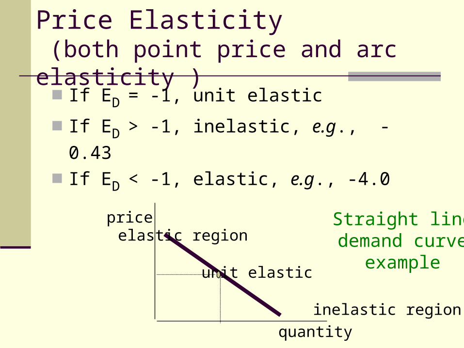
Price Elasticity (both point price and arc elasticity )

If ED = -1, unit elastic

If ED > -1, inelastic, e.g., - 0.43

If ED < -1, elastic, e.g., -4.0

priceelastic region

unit elastic

inelastic region

Straight linedemand curve

example

quantity

FIGURE 3.4 Perfectly Elastic and Inelastic Demand Curves

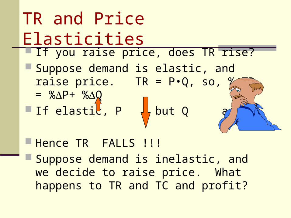
TR and Price Elasticities If you raise price, does TR rise? Suppose demand is elastic, and raise price.

TR = P•Q, so, %TR = %P+ %Q If elastic, P , but Q a lot

Hence TR FALLS !!! Suppose demand is inelastic, and we decide

to raise price. What happens to TR and TC and profit?

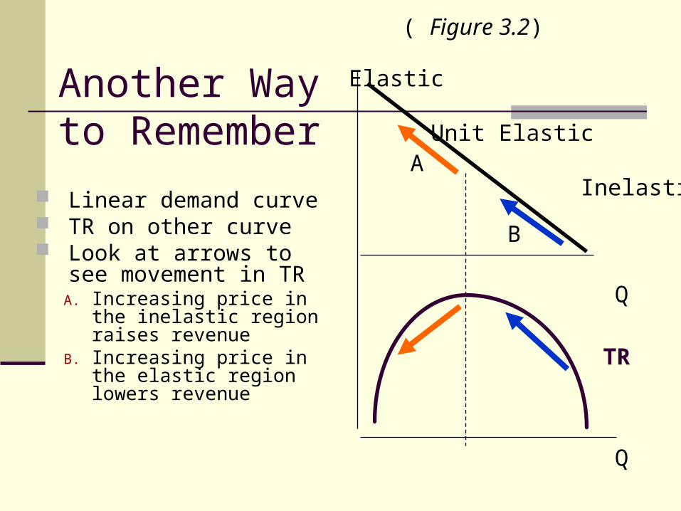
Another Way to Remember

Linear demand curve TR on other curve Look at arrows to

see movement in TRA. Increasing price in the

inelastic region raises revenue

B. Increasing price in the elastic region lowers revenue

Elastic

Unit Elastic

Inelastic

TR

Q

Q

( Figure 3.2)

A

B

FIGURE 3.5 Price Elasticity over Demand Function

FIGURE 3.5 Price Elasticity over Demand Function

MR and Elasticity

Marginal revenue is TR QTo sell more, often price must decline,

so MR is often less than the price. MR = P ( 1 + 1/ED )

For a perfectly elastic demand, ED = -B. Hence, MR = P.

If ED = -2, then MR = .5•P, or is half of the price.

1979 Deregulation of Airfares

Prices declined after deregulationAnd passengers increasedAlso total revenue increasedWhat does this imply about the price

elasticity of air travel?

It must be that air travel was elastic, as a price decrease after deregulation led to greater total revenue for the airlines.

Determinants of the Price Elasticity The availability and the closeness of substitutes

more substitutes, more elastic

The more durable is the product Durable goods are more elastic than non-durables

The percentage of the budget larger proportion of the budget, more elastic

The longer the time period permitted more time, generally, more elastic consider examples of business travel versus vacation travel

for all three above.

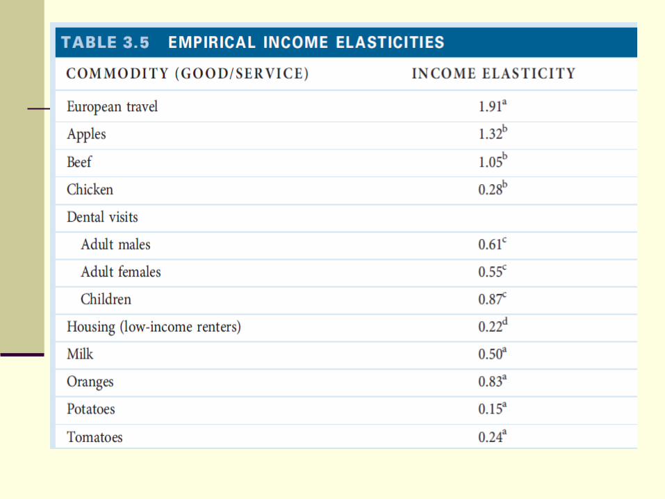
Empirical Price Elasticities

Apparel (whole market) -1.1

Apparel (one firm) -4.1 Beer -.84 Wine -.55 Liquor -.50 Regular coffee -.16 Instant coffee -.36 Adult visits to dentist

men -.65 Women -.78

Children visit to dentist -1.4

Furniture -3.04 Glassware & China -1.2 School lunches -.47 Flights to Europe -1.25 Shoes -.73 Soybean meal -1.65 Telephones -.10 Tires -.60 Tobacco -.46 Tomatoes -2.22 Wool -1.32

Free Trade and Price Elasticities

NAFTA (North American Free Trade Agreement) and Europe having a common currency in the Euro are examples of greater freedom in trade

What does that do to price elasticities? With more substitutes, we expect that

products become More Elastic Consumers gain as firms are less able to

raise their prices, but firm face stiffer competition

Income ElasticityEY = %Q/ %Y = (Q/Y)( Y/Q) point income

arc income elasticity: suppose dollar quantity of food expenditures of

families of $20,000 is $5,200; and food expenditures rises to $6,760 for families earning $30,000.

Find the income elasticity of food %Q/ %Y = (1560/5980)•(10,000/25,000) = .652 With a 1% increase in income, food purchases

rise .652%

EY = Q/ [(Q1 + Q2)/2] arc incomeY/ [(Y1 + Y2)/2] elasticity

Income Elasticity Definitions

If EY >0, then it is a normal or income superior good

some goods are Luxuries: EY > 1 with a high income elasticity

some goods are Necessities: EY < 1 with a low income elasticity

If EY is negative, then it’s an inferior good

Consider these examples:

1. Expenditures on new automobiles

2. Expenditures on new Chevrolets

3. Expenditures on 1996 Chevy Cavaliers with 150,000 miles

Which of the above is likely to have the largest income elasticity?

Which of the above might have a negative income elasticity?

Point Income Elasticity Problem

Suppose the demand function is:

Q = 10 - 2•P + 3•Y find the income and price elasticities at a price

of P = 2, and income Y = 10 So: Q = 10 -2(2) + 3(10) = 36

EY = (Q/Y)( Y/Q) = 3( 10/ 36) = .833

ED = (Q/P)(P/Q) = -2(2/ 36) = -.111

Characterize this demand curve, which means describe them using elasticity terms.

Advertising Elasticity

EA = %Q/ %ADV = (Q/ADV)( ADV/Q)

If the Advertising elasticity is .60, then a 1% increase in Advertising Expenditures increases the quantity of goods sold by .60%.

Cross Price Elasticities

EX = %QA / %PB = (QA/PB)(PB /QA)

Substitutes have positive cross price elasticities: Butter & Margarine

Complements have negative cross price elasticities: DVD machines and the rental price of DVDs at Blockbuster

When the cross price elasticity is zero or insignificant, the products are not related

Antitrust & Cross Price Elasticities Whether a product is a monopoly or in a

larger industry is dependent on the closeness of the substitutes

DuPont’s cellophane was at first viewed as a monopoly. Economists showed that the cross price elasticity with other products such as aluminum foil, waxed paper, and other flexible wrapping paper was Positive, the large, DuPont showed its cellophane was not a monopoly in this larger market.

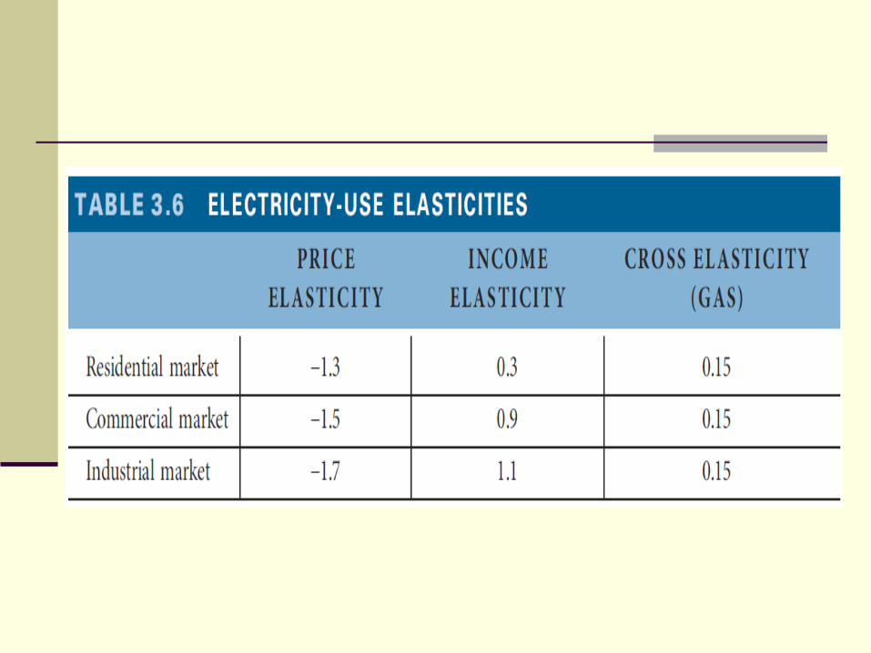
PROBLEM: Find the point price elasticity, the point income elasticity, and the point cross-price elasticity at P=10, Y=20, and Ps=9, if the demand function were estimated to be:

QD = 90 - 8·P + 2·Y + 2·Ps

Is the demand for this product elastic or inelastic? Is it a luxury or a necessity? Does this product have a close substitute or complement? Find the point elasticities of demand.

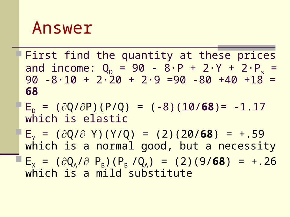
Answer First find the quantity at these prices and income:

QD = 90 - 8·P + 2·Y + 2·Ps = 90 -8·10 + 2·20 + 2·9 =90 -80 +40 +18 = 68

ED = (Q/P)(P/Q) = (-8)(10/68)= -1.17 which is elastic

EY = (Q/Y)(Y/Q) = (2)(20/68) = +.59 which is a normal good, but a necessity

EX = (QA/PB)(PB /QA) = (2)(9/68) = +.26 which is a mild substitute

Combined Effect of Demand Elasticities

Most managers find that prices and income change every year. The combined effect of several changes are additive.

%Q = ED(% P) + EY(% Y) + EX(% PR) where P is price, Y is income, and PR is the price of a related good.

If you knew the price, income, and cross price elasticities, then you can forecast the percentage changes in quantity.

Example: Combined Effects of Elasticities

Toro has a price elasticity of -2 for snow blowers Toro snow blowers have an income elasticity of 1.5 The cross price elasticity with professional snow

removal for residential properties is +.50 What will happen to the quantity sold if you raise price

3%, income rises 2%, and professional snow removal companies raises its price 1%? %Q = EP • %P +EY • %Y + Ecross • %PR = -2 • 3% + 1.5 •

2% +.50 • 1% = -6% + 3% + .5% %Q = -2.5%. We expect sales to decline 2.5%.

Q: Will Total Revenue for your product rise or fall?

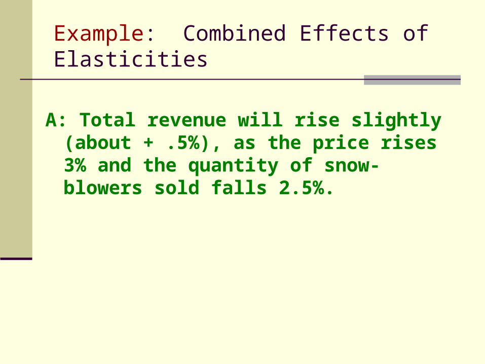
Example: Combined Effects of Elasticities

A: Total revenue will rise slightly (about + .5%), as the price rises 3% and the quantity of snow- blowers sold falls 2.5%.

OptimizationTechniques

Economic Optimization Process

Optimal Decisions Best decision helps achieve objectives most

efficiently. Maximizing the Value of the Firm

Value maximization requires serving customers efficiently.

What do customers want? How can customers best be served?

Expressing Economic Relations

Tables and Equations Simple graphs and tables are useful. Complex relations require equations.

Total, Average, and Marginal Relations Total increases when marginal is positive.

Revenue per time period ($)$9 8 7 6 5 4

3 Total revenue = $1.50 ´ output 2 1

0 1 2 3 4 5 6 7 8 9 Output per time period (units)

Maximization Occurs when Marginal Switches from Positive to Negative.

If marginal is above average, average is rising.

If marginal is below average, average is falling.

Graphing Total, Marginal, and Average Relations Deriving Totals from Marginal and Average

Curves Total is sum of marginal.

Marginal Analysis in Decision Making Use of Marginals in Resource Allocation

Maximum and minimum points occur where marginal is zero.

Distinguishing Maximums from Minimums Total and Marginal Relations

Maximizing the Difference Between Two Functions Maximum profit requires MR = MC. When profits are maximized, total profit decreases

with a change in output.

Practical Applications of Marginal Analysis Profit maximization requires Mπ = MR-MC = 0

and MR=MC and that π is falling as output expands.

Revenue maximization requires MR=0. Firms sometimes grab market share when

maximizing long-run profitability. Average cost minimization requires MC=AC

and that AC is rising as output expands.

Incremental Concept in Economic Analysis Marginal v. Incremental Concept

Marginal relates to one unit of output. Incremental relates to one managerial

decision. Multiple units of output is possible.

Incremental Profits Profits tied to a managerial decision.

Incremental Concept Example