ACTAUNIVERSITATIS

UPSALIENSISUPPSALA

2016

Digital Comprehensive Summaries of Uppsala Dissertationsfrom the Faculty of Science and Technology 1444

Demagnetization and FaultSimulations of Permanent MagnetGenerators

STEFAN SJÖKVIST

ISSN 1651-6214ISBN 978-91-554-9733-0urn:nbn:se:uu:diva-303517

Dissertation presented at Uppsala University to be publicly examined in Häggsalen,Ångströmlaboratoriet, Lägerhyddsvägen 1, Uppsala, Friday, 9 December 2016 at 09:15 forthe degree of Doctor of Philosophy. The examination will be conducted in English. Facultyexaminer: Dr. Sami Ruoho (Nordmag Oy).

AbstractSjökvist, S. 2016. Demagnetization and Fault Simulations of Permanent Magnet Generators.Digital Comprehensive Summaries of Uppsala Dissertations from the Faculty of Science andTechnology 1444. 59 pp. Uppsala: Acta Universitatis Upsaliensis. ISBN 978-91-554-9733-0.

Permanent magnets are today widely used in electrical machines of all sorts. With their increasein popularity, the amount of research has increased as well. In the wind power project at UppsalaUniversity permanent magnet synchronous generators have been studied for over a decade.However, a tool for studying demagnetization has not been available. This Ph.D. thesis coversthe development of a simulation model in a commercial finite element method software capableof studying demagnetization. Further, the model is also capable of simulating the connectedelectrical circuit of the generator. The simulation model has continuously been developedthroughout the project. The simulation model showed good agreement compared to experiment,see paper IV, and has in paper III and V successfully been utilized in case studies. The mainfocus of these case studies has been different types of short-circuit faults in the electrical systemof the generator, at normal or at an elevated temperature. Paper I includes a case study with thelatest version of the model capable of handling multiple short-circuits events, which was notpossible in earlier versions of the simulation model. The influence of the electrical system onthe working point ripple of the permanent magnets was evaluated in paper II. In paper III andVI, an evaluation study of the possibility of creating a generator with an interchangeable rotoris presented. A Neodymium-Iron-Boron (Nd-Fe-B) rotor was exchanged for a ferrite rotor withthe electrical properties almost maintained.

Keywords: Demagnetization, Permanent magnet, Finite Element Method, Synchronousgenerators, Wind power

Stefan Sjökvist, Department of Engineering Sciences, Electricity, Box 534, UppsalaUniversity, SE-75121 Uppsala, Sweden.

© Stefan Sjökvist 2016

ISSN 1651-6214ISBN 978-91-554-9733-0urn:nbn:se:uu:diva-303517 (http://urn.kb.se/resolve?urn=urn:nbn:se:uu:diva-303517)

Not so permanent now are you, permanent magnet?

List of papers

This thesis is based on the following papers, which are referred to in the textby their Roman numerals.

I S. Sjökvist and S. Eriksson, "Investigation of Permanent MagnetDemagnetization in Synchronous Machines During MultipleShort-Circuit Fault Conditions", Submitted to IET Renewable PowerGeneration, September 2016.

II S. Sjökvist, M. Rossander and S. Eriksson, "Permanent MagnetWorking Point Ripple in Synchronous Generators", Submitted to IETJournal of Engineering, October 2016.

III S. Sjökvist, P. Eklund and S. Eriksson, "Determining DemagnetisationRisk for Two PM Wind Power Generators with Different PM Materialand Identical Stators", IET Electric Power Applications, vol. 10, no. 7,pp. 593-597, August 2016.

IV S. Sjökvist and S. Eriksson, "Experimental Verification of a SimulationModel for Partial Demagnetization of Permanent Magnets", IEEETransactions on Magnetics, vol. 50, no. 12, pp. 1-5, December 2014.

V S. Sjökvist and S. Eriksson, "Study of Demagnetization Risk for a12 kW Direct Driven Permanent Magnet Synchronous Generator forWind Power", Energy Science and Engineering, vol. 1, no. 3, pp.128-134, September 2013.

VI P. Eklund, S. Sjökvist, S. Eriksson and M. Leijon, "A CompleteDesign of a Rare Earth Metal-Free Permanent Magnet Generator",Machines, vol. 2(2), pp. 120-133, May 2014.

Reprints were made with permission from the publishers.

Other contributions:A The author presented parts of the work from paper V at the conference

Magnetic Materials in Electrical Machine Applications 2012 in Pori,Finland, 13-15 June 2012.

B L. Sjökvist, J. Engström, S. Larsson∗, M. Rahm, J. Isberg and M. Lei-jon, "Simulation of Hydrodynamical Forces on a Buoy - a ComparisonBetween Two Computational Approaches", In Proceedings of the 1stAsian Wave and Tidal Energy Conference Series, Jeju, South Korea, 27-30 November 2012.

∗The author changed his surname from Larsson to Sjökvist in July 2013.

Contents

Nomenclature . . . . . . . . . . . . . . . . . . . . . . . . . . . . . . . . . . . . . . . . . . . . . . . . . . . . . . . . . . . . . . . . . . . . . . . . . . . . . . . . . . . . . . . . . . . . . . . . . . . . ix

List of Abbreviations . . . . . . . . . . . . . . . . . . . . . . . . . . . . . . . . . . . . . . . . . . . . . . . . . . . . . . . . . . . . . . . . . . . . . . . . . . . . . . . . . . . . . . . . xi

1 Introduction . . . . . . . . . . . . . . . . . . . . . . . . . . . . . . . . . . . . . . . . . . . . . . . . . . . . . . . . . . . . . . . . . . . . . . . . . . . . . . . . . . . . . . . . . . . . . . . . 131.1 History of the wind power project . . . . . . . . . . . . . . . . . . . . . . . . . . . . . . . . . . . . . . . . . . . . . . . . 141.2 Aim of this thesis . . . . . . . . . . . . . . . . . . . . . . . . . . . . . . . . . . . . . . . . . . . . . . . . . . . . . . . . . . . . . . . . . . . . . . . . . . . 16

2 Theory . . . . . . . . . . . . . . . . . . . . . . . . . . . . . . . . . . . . . . . . . . . . . . . . . . . . . . . . . . . . . . . . . . . . . . . . . . . . . . . . . . . . . . . . . . . . . . . . . . . . . . . . 172.1 Magnetic materials . . . . . . . . . . . . . . . . . . . . . . . . . . . . . . . . . . . . . . . . . . . . . . . . . . . . . . . . . . . . . . . . . . . . . . . . . 17

2.1.1 Classification of magnetic materials . . . . . . . . . . . . . . . . . . . . . . . . . . . . . . 172.1.2 Magnetism on a macroscopic level . . . . . . . . . . . . . . . . . . . . . . . . . . . . . . . . 182.1.3 Soft ferromagnetic materials . . . . . . . . . . . . . . . . . . . . . . . . . . . . . . . . . . . . . . . . . . . 202.1.4 Hard ferromagnetic materials . . . . . . . . . . . . . . . . . . . . . . . . . . . . . . . . . . . . . . . . . 20

2.2 The finite element method . . . . . . . . . . . . . . . . . . . . . . . . . . . . . . . . . . . . . . . . . . . . . . . . . . . . . . . . . . . . . 212.2.1 Derivation of the transient field equation . . . . . . . . . . . . . . . . . . . . . . . 222.2.2 Boundary conditions . . . . . . . . . . . . . . . . . . . . . . . . . . . . . . . . . . . . . . . . . . . . . . . . . . . . . . . 232.2.3 Modeling of the B-H-curve and the recoil line . . . . . . . . . . . . . . 24

3 Methods . . . . . . . . . . . . . . . . . . . . . . . . . . . . . . . . . . . . . . . . . . . . . . . . . . . . . . . . . . . . . . . . . . . . . . . . . . . . . . . . . . . . . . . . . . . . . . . . . . . . . . 273.1 Simulating with COMSOL Multiphysics . . . . . . . . . . . . . . . . . . . . . . . . . . . . . . . . . . . . . 273.2 Development of demagnetization model . . . . . . . . . . . . . . . . . . . . . . . . . . . . . . . . . . . . . . 283.3 Experimental verification of stationary demagnetization model 31

3.3.1 Experimental Set-up . . . . . . . . . . . . . . . . . . . . . . . . . . . . . . . . . . . . . . . . . . . . . . . . . . . . . . . . 313.3.2 Measuring the magnetic flux density . . . . . . . . . . . . . . . . . . . . . . . . . . . . . 323.3.3 Experiments . . . . . . . . . . . . . . . . . . . . . . . . . . . . . . . . . . . . . . . . . . . . . . . . . . . . . . . . . . . . . . . . . . . . . 34

3.4 Evaluation of the two time-dependent demagnetization models 343.4.1 Electrical circuit . . . . . . . . . . . . . . . . . . . . . . . . . . . . . . . . . . . . . . . . . . . . . . . . . . . . . . . . . . . . . . . 343.4.2 Transient analysis . . . . . . . . . . . . . . . . . . . . . . . . . . . . . . . . . . . . . . . . . . . . . . . . . . . . . . . . . . . . 353.4.3 Comparison with stationary model . . . . . . . . . . . . . . . . . . . . . . . . . . . . . . . . . 37

3.5 Ripple in surface mounted permanent magnets . . . . . . . . . . . . . . . . . . . . . . . . . . . 373.6 Comparison of ferrite and Nd-Fe-B rotor . . . . . . . . . . . . . . . . . . . . . . . . . . . . . . . . . . . . . 37

4 Summary of results and discussion . . . . . . . . . . . . . . . . . . . . . . . . . . . . . . . . . . . . . . . . . . . . . . . . . . . . . . . . . . 394.1 Experimental verification . . . . . . . . . . . . . . . . . . . . . . . . . . . . . . . . . . . . . . . . . . . . . . . . . . . . . . . . . . . . . . 394.2 Time-dependent models . . . . . . . . . . . . . . . . . . . . . . . . . . . . . . . . . . . . . . . . . . . . . . . . . . . . . . . . . . . . . . . . . 414.3 Ripple in permanent magnets . . . . . . . . . . . . . . . . . . . . . . . . . . . . . . . . . . . . . . . . . . . . . . . . . . . . . . . . 434.4 The ferrite alternative . . . . . . . . . . . . . . . . . . . . . . . . . . . . . . . . . . . . . . . . . . . . . . . . . . . . . . . . . . . . . . . . . . . . . 44

5 Conclusions . . . . . . . . . . . . . . . . . . . . . . . . . . . . . . . . . . . . . . . . . . . . . . . . . . . . . . . . . . . . . . . . . . . . . . . . . . . . . . . . . . . . . . . . . . . . . . . . 47

6 Summary of Papers . . . . . . . . . . . . . . . . . . . . . . . . . . . . . . . . . . . . . . . . . . . . . . . . . . . . . . . . . . . . . . . . . . . . . . . . . . . . . . . . . . . . 49

7 Svensk sammanfattning . . . . . . . . . . . . . . . . . . . . . . . . . . . . . . . . . . . . . . . . . . . . . . . . . . . . . . . . . . . . . . . . . . . . . . . . . . . . . 52

8 Acknowledgements . . . . . . . . . . . . . . . . . . . . . . . . . . . . . . . . . . . . . . . . . . . . . . . . . . . . . . . . . . . . . . . . . . . . . . . . . . . . . . . . . . . 54

References . . . . . . . . . . . . . . . . . . . . . . . . . . . . . . . . . . . . . . . . . . . . . . . . . . . . . . . . . . . . . . . . . . . . . . . . . . . . . . . . . . . . . . . . . . . . . . . . . . . . . . . . 55

Nomenclature

Symbol SI Unit Quantity

A Wb/m Magnetic vector potentialAz Wb/m Magnetic vector potential, z-componentAdest

z Wb/m Magnetic vector potential on the destination boundary, z-component

Asrcz Wb/m Magnetic vector potential on the source boundary, z-

componentB T Magnetic flux densityBHmax J/m3 Maximum energy productBmin T Minimum magnetic flux densityB|| T Magnetic flux density parallel to the magnetization directionBr T RemanenceBnew

r T New remanenceBprev

r T Remanence from the previous iterationBs T Saturation of the magnetic flux densityBprev

y T Magnetic flux density, y-component, from the previous iter-ation

CDC F Capacitance on the DC-linkD C/m2 Electric displacement fieldE V/m Electric fieldfel Hz Electrical frequencyH A/m Magnetic fieldHc A/m CoercivityHcJ A/m Intrinsic coercivityHmin A/m Minimum magnetic fieldH prev

y A/m Magnetic field, y-component, from the previous iterationI A CurrentID A Diode currentIm T Magnetic polarization or intensity of magnetizationIS A Reverse bias saturation currentJ A/m2 Current densityJ f A/m2 Free current densityJm A/m2 Magnetization current densityk Vs/Am Slope of the B-H-curveK1 m/A Knee point shape parameterkB J/K Boltzmann constantkBr %/K Temperature coefficient for the remanence

Continued on next page

Symbol SI Unit Quantity

kHcJ %/K Temperature coefficient for the intrinsic coercivityL H Generator inductance per phaseM A/m MagnetizationMs A/m Saturation magnetizationq C Magnitude of the charge of an electronR Ω Generator resistance per phaseRab Ω Short-circuit resistance between phase a and bRbc Ω Short-circuit resistance between phase b and cRDC Ω Short-circuit resistance over the load on the DC sideRL Ω Resistance loadRs Ω Snubber resistanceT K Absolute temperatureTre f K Listed reference temperatureu − Solution to the ODEva, vb, vc V Generator output line-neutral voltages of phase a, b and cVD V Diode voltageEa, Eb, Ec V Generator electromotive force of phase a, b and cφ V Electric potentialϕm

Angle between the magnetization and the applied fieldµ0 Vs/Am Permeabilityµr − Relative permeabilityσ A/Vm Electric conductivityχm − Susceptibility

List of Abbreviations

Abbrevation Description

2D Two dimensional3D Three dimensionalAC Alternating currentCM COMSOL Multiphysics R©

DC Direct-currentDDPMSG Direct driven permanent magnet synchronous generatorDLL Dynamic-link libraryFEM Finite element methodNd-Fe-B Neodymium-Iron-BoronODE Ordinary differential equationPM Permanent magnetPMSG Permanent magnet synchronous generatorPMSM Permanent magnet synchronous machineRD Rolling directionSm-Co Samarium-CobaltTD Transverse directionVAWT Vertical axis wind turbineVCCS Voltage-controlled current source

1. Introduction

Permanent magnets (PMs) are widely used as the field source in electricalmachines and compared to electrically excited machines there are no lossesin the excitation system which results in higher efficiency and higher outputpower per volume of machine [1–7]. When designing an electrical machinethe design goals are; to optimize the use of the magnetic flux density (B) bya suitable selection of both hard and soft magnetic materials, to maximizethe interaction between the magnetic flux density and the stator windings byoptimizing the geometry, and to minimize losses such as eddy-current, hys-teresis and frictional losses. The most recent big step in PM development waswith the introduction of the Neodymium-Iron-Boron (Nd-Fe-B) PMs in the1980’s [8, 9], not to say that PMs have not developed since then. There isongoing research on the material design of PMs trying to increase both theirability to produce high fields and withstand high fields without being partiallydemagnetized [10, 11].

Since permanent magnet synchronous machines (PMSMs) are widely usedand have a long expected lifespan, a machine is therefore likely to be exposedto one or several faults during its lifetime. Faults in PMSM can be dividedinto stator faults, rotor faults, and bearing faults. If the machine is connectedto an inverter, faults in the switches and the sensors may also occur. Faultson the rotor side may be caused, for example, by eccentricity, damage in oneor more permanent magnets, asymmetries, or mechanical looseness. For thestator, a cause of failure may be winding insulation breakdown, asymmetriesor mechanical looseness [12–15]. There are several methods for detecting andpredicting faults, e.g. by monitoring the mechanical vibrations, the temper-ature, the insulation degradation, the power output, and/or the current [12].Current monitoring is a widely spread technique which can be used on ma-chines in production environments for continuous monitoring. The spectrumof the current is analysed to determine abnormal frequency components dueto, for example, air gap eccentricity or partial demagnetization [12, 16–18].

In any machine design process, consideration needs to be put into toler-ances and material properties to make sure the machine can be assembled andcan manage the mechanical stresses. The same needs to be done regardingthe electromagnetic properties. In the same way the mechanical constructionneeds to be able to withstand some abnormal conditions, the electromagneticproperties needs to be maintained after, e.g. an overload situation and/or a situ-ation of increased temperature. The demagnetization risk should be analysed,at least, for normal working conditions and some expected overload condi-tions. Preferably, the most common fault conditions should also be analysed.

13

The arguments for not considering all possible fault conditions is the cost,however, if the most severe case do happen, replacement of the whole ma-chine may be necessary anyway. [19–21]

With the increasing popularity of PM electrical machines the amount ofstudies on demagnetization has increased as well. In the 1980s and 1990s,there were several studies on the influence of grain orientation alignment onthe coercivity and the angular dependence of an applied field [22–27]. Inthese studies, one focus was to try to describe and present models for the grainorientations influence on the intrinsic coercivity and the remanence of the per-manent magnets. Roughly, the trend was a 1/cosϕm relationship, where ϕm isthe angle between the magnetization (M) and the applied magnetic field (H).However, the results do not seem to converge to a general angular dependencerelationship. There are simply too many factors involved, such as the materialcomposition, grain size, and different alignment field strengths and pressingdirections during the sintering process.

Since the 2000s, the research focus has shifted a bit, from the influence ofthe grain orientation, to more focus on case studies on actual machines anddesign optimization [21, 28–31]. However, there is still research performedon the inclined field topic [32]. For example, Ruoho presented a demagneti-zation model taking the angular dependence into account using an empiricalmodel [33]. While this is the simplest model to implement in a finite elementmethod (FEM) model the author has come across, since it consists only of theintrinsic coercivity (HcJ), a third-degree polynomial, and ϕm, it is still an em-pirical model suitable for a limited set of Nd-Fe-B PMs. While, to the author’sknowledge, a general model is yet to exist, this polynomial model may be thebest option for designers of PM machines.

1.1 History of the wind power projectThe work presented in this Ph.D. thesis is a part of the wind power researchproject at the division for electricity, Uppsala University [34]. The wind powerproject started in 2002 with the vision of developing a mechanically simpleand low maintenance wind power concept. The vision resulted in an ideawith a vertical axis wind turbine (VAWT), more specific a Darrieus H-typerotor. The H rotor is omnidirectional and can, therefore, extract energy fromthe wind regardless of the wind direction making a yaw system unnecessary.The turbine is passive stall regulated. The turbine connects, via its shaft, to adirect driven permanent magnet synchronous generator (DDPMSG) placed atground level. The possibility to install the generator and other heavy compo-nents at ground level reduces stress on the tower which allows for a slendertower construction, giving the system a low center of mass which is preferablein e.g. floating offshore wind applications. Installing the generator and othercomponents at ground level also enables easier access during maintenance.

14

Figure 1.1. A vertical axis H-type wind turbine connected to a 12 kW DDPMSGdesigned and built within the wind power project.

The wind power group have to date designed and produced three full windpower plants (turbine and generator), and one lab generator. The lab genera-tor was recently converted from using a surface mounted NdFeB rotor to thepresent spoke type ferrite rotor. Figure 1.1 shows a vertical axis wind tur-bine connected to a 12 kW DDPMSG, which was built within the wind powerproject.

Previous work from the group has focused on the wind power system andthe properties of the generator [35–37], as well as aerodynamics and soundpollution [38–41].

Here follows a summary of the most recent studies by the wind powergroup. Eklund has performed studies on the mechanical design and the pos-sible use of rare earth metal-free alternatives to the Nd-Fe-B PMs previouslyused [42]. Rossander has performed measurements of the blade forces of the12kW prototype and studied how oscillations propagate through the turbineas well as how passive rectification of the generator affects the turbine [43].Olauson has in [44] studied and modeled the variability and forecasting of re-newable energy sources, and their influence on the power system. Apelfröjdhas made extensive research on the grid connection, electrical system, andcontrol system for the wind turbine [45]. He has also written a comprehen-sive review of the previous work done by the wind power group over the lastdecade [34].

15

While extensive work previously has been done regarding the generatordesign, a tool for studying demagnetization of permanent magnets has notbeen available. Therefore, design optimization has not been possible to thesame extent as if a tool for studying demagnetization had been available. Ademagnetization model would, therefore, be beneficial for the future generatordesign and generator-VAWT interaction research.

1.2 Aim of this thesisThe aim of this thesis is to study and model demagnetization of permanentmagnets by, firstly, developing an easy to use simulation model which requirelittle hands-on application by the user.

A secondary objective is to build the entire model in commercially avail-able software. In the majority of the references in the Introduction section, thesimulation software was either not mentioned or proprietary. Using a com-mercially available software may have some limitations in the user’s ability toimplement specific features. But for research progress to become easily avail-able in the industry, it is important to prove that it is possible to implementspecial features/functions in commercial available software and not only inproprietary software.

Finally, a third goal is to demonstrate and experimentally verify the simu-lation model.

16

2. Theory

2.1 Magnetic materialsThe magnetic material used in an electrical machine is more than just the PMmaterial. The magnetic materials in an electrical machine include both thePMs and all the material used to complete the machine’s magnetic circuit,usually called the active material. This section gives a brief introduction to thedifferent magnetic material classifications and their properties [46–48].

2.1.1 Classification of magnetic materialsThe macroscopic magnetic properties of materials are a consequence of themagnetic moments of the electrons in individual atoms. Each electron’s mag-netic moment originates from two sources. One is the electron’s orbital motionaround the nucleus, and the other is the electron’s spin. The magnetic momentof the orbital motion can be considered a small current loop, having its mag-netic moment along the axis of rotation. Each electron can either have a spinup or spin down and the magnetic moment is pointing along the spin axis. Ineach atom, the individual orbital magnetic moments of the electrons can can-cel each other out; this is also the case for the spin magnetic moment. Anelectron cancels the spin magnetic moment of an electron with a spin up, witha spin down. The net magnetic moment of an electron is, therefore, the sum ofthe contributions of all electrons of the atom. For an atom having filled innerand outer shells, there is total cancellation of both orbital and spin magneticmoments. These materials are not able to be permanently magnetized.

The three common types of magnetism are diamagnetism, paramagnetism,and ferromagnetism. There are further categories which usually are consid-ered being subclasses of ferromagnetism; these subclasses will not be dis-cussed. All materials exhibit at least one of these three types, depending ontheir electrons response to an externally applied magnetic field.

DiamagnetismDiamagnetism is a weak form of magnetism only present when an externalmagnetic field is applied. With the application of an external magnetic field,the orbital motion of the electrons is deranged causing a change in the totalmagnetic moment of the atom. The change is small, and the atom’s magneticfield is always pointing in the opposite direction of the external field. Dia-magnetism is present in all materials but can only be observed when all otherforms of magnetism are absent since the effect is so small.

17

ParamagnetismFor materials with an incomplete cancellation of the atoms’ magnetic moment,a net magnetic moment of each atom will remain even in the absence of an ex-ternal magnetic field. However, the orientation of these magnetic moments israndomized, such that the material does not possess a net macroscopic mag-netization. These magnetic moments are free to rotate, and when aligned byan external field, the effect is called paramagnetism. The magnetic dipole ofeach atom is individually affected and brought into line with an external field,and there is no interaction between adjacent dipoles. Both diamagnetic andparamagnetic materials are considered non-magnetic since an external field isrequired for them to show their magnetic behavior.

FerromagnetismThe characteristic of ferromagnetism is when a material on a macroscopicscale can possess a net magnetization in the absence of an applied magneticfield. Ferromagnetism is probably the most well known magnetic materialclassification since its properties are easily observable without any measure-ment equipment. The main contribution to the great permanent magnetic mo-ment of ferromagnetic materials is the uncanceled spin contributions, as a con-sequence of the beneficial electron structure. There is an orbital magnetic mo-ment contribution, but it is small in comparison to the magnetic moment fromthe electron spin. Further, there is a coupling factor between the atoms mag-netic moments which allow for the alignment of the magnetic moments. Thisalignment exists over relatively large areas; these regions where the magneticmoment is aligned in the same direction are called magnetic domains.

The maximum magnetization possible, or saturation magnetization (Ms), isachieved when the alignment of all magnetic domains is in the same direction.The saturation magnetization is the product of the magnetic moment of eachatom and the number of atoms present in the structure.

2.1.2 Magnetism on a macroscopic levelAs briefly described in the previous section, the resulting magnetization field,M, from all magnetic moments in a material is the sum of contributions fromall magnetic dipoles of the structure. Since each atom has a net current due tothe moving and spinning of its electrons, the current from all the atoms in alimited space can be considered a current density. This current density can bedetermined by

Jm = ∇×M, (2.1)

where, Jm is the magnetization current density. B is determined by currentdensities of all kinds, which at low frequencies (neglecting the displacementcurrent density) is defined by Ampere-Maxwell’s law as

∇×B = µ0J = µ0(J f +Jm), (2.2)

18

where, µ0 is the permeability and J f is the free current density. Combining2.2 with the constitutive relation

B = µ0(H+M), (2.3)

the following is obtained∇×H = J f . (2.4)

Which is the Ampere-Maxwell equation for the magnetic field. Equation 2.3is often used to model the properties of PMs in FEM simulations. Further, Mis proportional to H as

M = χmH, (2.5)

where, χm is called the susceptibility. The susceptibility can also be written as

χm = µr−1, (2.6)

where, µr is the relative permeability of the material. Combining Equation 2.3,2.5 and 2.6 one eventually arrives at

B = µ0µrH (2.7)

which is another constitutive relation, often used to describe soft magneticmaterials such as electrical steel for stator and transformer cores. Please notethat the relative permeability is not necessarily a constant.

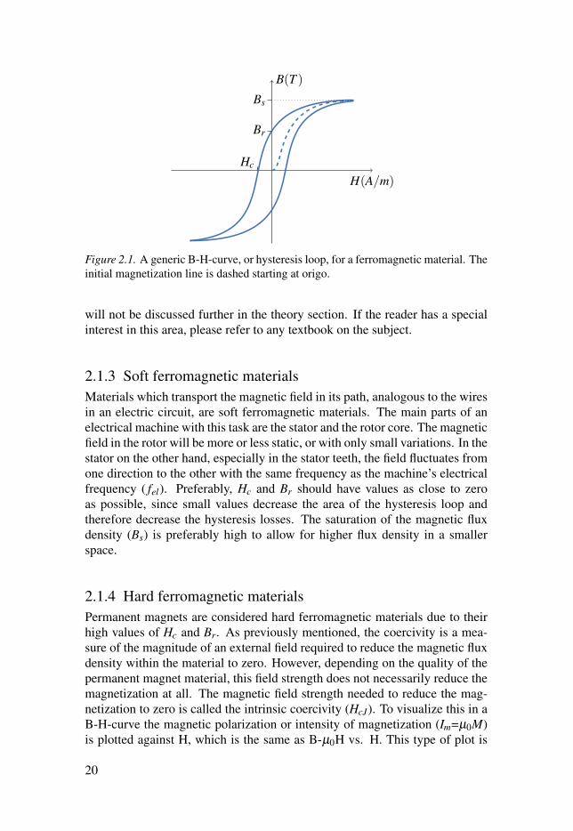
The properties of ferromagnetic materials can vary significantly betweendifferent materials, which make some of them ideal for electric power appli-cations. Significant for ferromagnetic materials, compared to diamagnetic andparamagnetic materials is their highly non-linear relative permeability. Therelative permeability and the ability to be permanently magnetized depend onseveral factors, e.g. material composition, temperature and the previous valueof the applied magnetic field. The non-linearity of µr becomes clearly visiblein a B-H-curve. Ferromagnetic materials are usually characterized by their sat-uration B-H-curve since much information can be extracted from this graph.A generic B-H-curve is shown in Figure 2.1, where the slope of the curve atany point is µ0µr. The dashed part is the initial magnetization curve, i.e. thecurve of a previously non-magnetized material. When the applied magneticfield becomes high enough the material becomes saturated. When the appliedmagnetic field is removed, some magnetic domains will not rotate back, anda resulting B will be left in the material. The remaining B is called the rema-nence (Br). For a ferromagnetic material subjected to a fluctuating magneticfield like in Figure 2.1 the hysteresis effect, or hysteresis loop, is clearly vis-ible. As can be seen in the figure, it is not sufficient to remove the appliedfiled to reduce B inside the material to zero. A field in the opposite directionis needed and the field strength needed is called the coercivity (Hc). The areawithin the hysteresis loop is a measure of how much extra energy is required tocomplete a full revolution of the B-H-curve, i.e. the hysteresis losses. Losses

19

H(A/m)

B(T )

Bs

Br

Hc

Figure 2.1. A generic B-H-curve, or hysteresis loop, for a ferromagnetic material. Theinitial magnetization line is dashed starting at origo.

will not be discussed further in the theory section. If the reader has a specialinterest in this area, please refer to any textbook on the subject.

2.1.3 Soft ferromagnetic materialsMaterials which transport the magnetic field in its path, analogous to the wiresin an electric circuit, are soft ferromagnetic materials. The main parts of anelectrical machine with this task are the stator and the rotor core. The magneticfield in the rotor will be more or less static, or with only small variations. In thestator on the other hand, especially in the stator teeth, the field fluctuates fromone direction to the other with the same frequency as the machine’s electricalfrequency ( fel). Preferably, Hc and Br should have values as close to zeroas possible, since small values decrease the area of the hysteresis loop andtherefore decrease the hysteresis losses. The saturation of the magnetic fluxdensity (Bs) is preferably high to allow for higher flux density in a smallerspace.

2.1.4 Hard ferromagnetic materialsPermanent magnets are considered hard ferromagnetic materials due to theirhigh values of Hc and Br. As previously mentioned, the coercivity is a mea-sure of the magnitude of an external field required to reduce the magnetic fluxdensity within the material to zero. However, depending on the quality of thepermanent magnet material, this field strength does not necessarily reduce themagnetization at all. The magnetic field strength needed to reduce the mag-netization to zero is called the intrinsic coercivity (HcJ). To visualize this in aB-H-curve the magnetic polarization or intensity of magnetization (Im=µ0M)is plotted against H, which is the same as B-µ0H vs. H. This type of plot is

20

−1.4 −1.2 −1 −0.8 −0.6 −0.4 −0.2 0

·106

−1.5

−1

−0.5

0

0.5

1

1.5

Intrinsic

NormalHcJ

Hc

H (A/m)

Bor

I m(T

)

Figure 2.2. Example of a normal and an intrinsic B-H-curve for a permanent magnet.

usually called an intrinsic B-H-curve. An example of a normal and intrinsicB-H-curve for a hard ferromagnetic material is shown in Figure 2.2.

All materials have some property which is temperature dependent and mag-netic materials are no exception. The temperature coefficient for the rema-nence (kBr) is generally negative, i.e. Br decreases when increasing the abso-lute temperature (T ). The temperature coefficient for the intrinsic coercivity(kHcJ) depends on the material. Ferrite permanent magnets have a positivetemperature coefficient, making them harder to demagnetize with increasingtemperature, whereas the opposite is true for other permanent magnet materi-als [49].

2.2 The finite element methodOne purpose of using finite element analysis on electrical machines is to cal-culate the magnetic field distribution inside the machine. This distribution canbe used to calculate other properties such as the induced voltage of the ma-chine. For symmetry reasons, it is usually sufficient to model a limited part ofthe machine. Depending on the size of the machine and the desired accuracyof the study, it is in many cases adequate to reduce the problem from a threedimensional (3D) to a two dimensional (2D) problem. An example machineof such a case is shown in Figure 2.3, which is the 12 kW permanent mag-net synchronous generator (PMSG) studied in Paper III and V where only thesmallest symmetrical part is modeled. Solving a 3D problem in 2D has somedrawbacks, 3D effects such as eddy currents and end effects of the machinecan not be modeled with full accuracy.

21

AirFeSiCopperAluminiumPermanent magnet

Figure 2.3. 2D representation of the smallest symmetrical piece of the 12 kW PMSG.

2.2.1 Derivation of the transient field equation

Time-dependent magnetic problems can be described with the following dif-

ferential equations

∇ ·B = 0 (2.8)

∇×E =−∂B∂ t

(2.9)

∇×H = J f +∂D∂ t

(2.10)

where, E is the electric field, and D is the electric displacement field. As be-

fore, if the frequencies of the source currents are low, the displacement current

density (−∂D/∂ t) is close to zero and can, therefore, be neglected and Equa-

tion 2.10 becomes the same as Equation 2.4. B and H are related through the

constitutive relation in Equation 2.7. From definition, we know that

B = ∇×A (2.11)

where, A is called the magnetic vector potential. Inserting Equation 2.11 into

Equation 2.9 and performing some vector algebra one arrives at

E =−∂A∂ t−∇φ (2.12)

where, φ is the electric potential. We also know that

J f = σE (2.13)

22

where, σ is the electric conductivity. Combining Equation 2.7 with 2.10-2.13,and letting ∇ ·A = 0, one should arrive at

∇× (µ0µr)−1

∇×A =−σ∂A∂ t−σ∇φ . (2.14)

Assuming µr is constant, applying some vector algebra onto Equation 2.14,we obtain

σ∂A∂ t− (µ0µr)

−1∇

2A =−σ∇φ , (2.15)

which is the equation solved in a FEM software for time-dependent magneticproblems. For magneto-static problems all time-dependent terms are removedand Equation 2.15 is reduced to

−(µ0µr)−1

∇2A =−σ∇φ . (2.16)

The assumption that µr is (piecewise) constant implies that hysteresis effectsare neglected.

2.2.2 Boundary conditionsIn order for the field problem to be fully defined, boundary conditions haveto be defined on the boundaries of the geometry. Three different boundaryconditions have been used, which all will be given a short explanation assum-ing simulation in 2D. The first, set on the inner and outer boundaries of theexample geometry is the homogeneous Dirichlet boundary condition

Az = 0 (2.17)

where, Az is the magnetic vector potential, z-component. A homogeneousDirichlet boundary condition is equivalent to an insulating boundary condi-tion, e.g. no flux is allowed through the boundary.

In a perfectly round and concentric electrical machine, the geometry ex-hibits a consistent feature. The size of the simulated geometry can be reducedto the smallest repeatable part by including periodic continuity boundary con-ditions

Asrcz = Adest

z (2.18)

where, Asrcz and Adest

z represents the z-component of the magnetic vector po-tential on the source and destination boundaries, respectively. The periodicboundary condition relates the value of Az on two equivalent boundaries toeach other, i.e. the flux passing through the source boundary will come backthrough the destination boundary.

The last boundary condition used is a sector symmetry boundary conditionor moving boundary condition, which is set on the boundary that representsthe air gap between the rotor and the stator. The sector symmetry boundary

23

Figure 2.4. The solid, dashed and dotted lines represent sector symmetry, homoge-neous Dirichlet and periodic boundary conditions, respectively. Paper V

condition works in a similar way as the periodic boundary condition with theaddition of allowing movement (without re-meshing) along the boundary. In acircular machine, the periodic boundary condition would be set on boundarieswith a surface normal parallel to the ϕ in a standard cylindrical coordinate sys-tem and the sector symmetry boundary condition would be set on boundarieswith a surface normal unit vector parallel to r.

2.2.3 Modeling of the B-H-curve and the recoil lineTo successfully model the demagnetization of permanent magnets a B andH relationship is required. Depending on how the permanent magnets aremodeled, M and the constitutive relation in Equation 2.3 might be needed aswell. Ideally, the B-H relationship is provided by the manufacturer. If not, aB-H-curve can be modeled with an analytical function [50]

B = Br +µ0µrH +EeK1(K2+H) (2.19)

where, E is a unit conversion factor of 1 T. The parameter K2 is calculatedfrom

K2 =ln[(Br +(µr−1) ·µ0 ·HcJ) ·E−1

]K1

−HcJ (2.20)

and the K1 parameter sets the shape of the knee point in the B-H-curve, wherea larger value gives a sharper knee. The author found good agreement withseveral Nd-Fe-B magnet grades with a K1 value of −1.5 · 10−4 m/A. Themagnetization can then be calculated with Equation 2.3.

24

−1 −0.8 −0.6 −0.4 −0.2 0

·106

−1.5

−1

−0.5

0

0.5

1

1.5

Hc•

HcJ•

Br•

Magnetic field (A/m)

Mag

netic

flux

dens

ity(T

)

StraightExponential

Figure 2.5. Comparison of the exponential model and the straight line model forreproducing B-H-curves.

An alternative and more straight forward way of modeling a B-H-curve areby using two straight lines. This approach has been tested against the methodpresented above with good results [51], at least for permanent magnets withvery sharp knees, which many Nd-Fe-B permanent magnets have. With thismethod a straight line with the slope

k = µ0µr (2.21)

is drawn from the Br. The second line is a straight line through Hc and HcJ thatwill coincide with the first line at the knee. A comparison of the two methodsis presented in Figure 2.5.

Since manufacturers often provide the temperature coefficient for the rema-nence and the coercivity, it is easy to reproduce a B-H-curve for any tempera-ture using

Br(T ) = Br(Tre f )(1+ kBr · (T −Tre f )), (2.22)HcJ(T ) = HcJ(Tre f )(1+ kHcJ · (T −Tre f )) (2.23)

where, Tre f is the listed reference temperature for the material properties ofthe permanent magnet.

When demagnetization has occurred and the applied magnetic field is re-moved, the recoil line will bend somewhat upwards when the applied fieldapproaches zero [33, 50]. However, this is often neglected to simplify analy-sis [52]. By doing so, the recoil line can be approximated by a straight line

25

with the same slope as the initial part of the B-H-curve, as in Equation 2.21.The new remanence (Bnew

r ) can, therefore, be expressed as

Bnewr = Bmin− kHmin (2.24)

where, Bmin and Hmin are the minimum magnetic flux density and magneticfield, respectively. The recoil will therefore follow the line

B = k(H−Hmin)+Bmin. (2.25)

26

3. Methods

This chapter will cover the methods used and the demagnetization model de-veloped during this project. The generators in the case studies was of a similarkind. All of them are modified versions of the 12 kW lab generator in Fig-ure 2.3 i.e. slow rotating multi-pole machines with relatively low load angle,and with surface mounted PMs, except for one which had a rotor with buriedferrite magnets. The chapter will begin with a section about the simulationsoftware used in all papers.

3.1 Simulating with COMSOL MultiphysicsThe following section will briefly describe the structure of the FEM softwareCOMSOL Multiphysics R©1 (CM). The software includes several physics mod-ules; each module provides a relevant set of options regarding loads, boundarycondition and initial values for that specific physics application. In this way,the user can add all the relevant physics modules needed, and skip those whichare not necessary or considered negligible. These physics modules can, if de-sired, be set-up to be coupled to one another. For example, leading a currentthrough an electrical conductor will generate heat which not will be consid-ered if only the module for electric currents is used. However, when the heattransfer module is added, the resistivity of the conducting material can be cou-pled to the temperature, and now the resistivity will change depending on thetemperature of the conducting material. Further, in many cases, there are mod-ules which are very similar. When simulating magnetic fields, for example, thebase module is called magnetic fields (mf). With the mf module, the user canperform a vast variety of simulations on magnetic fields. However, there isanother module called rotating machinery, magnetic (rmm), this module hassome preset properties for, as the name suggests, simulating rotating electricalmachines. Everything that can be done in rmm can also be accomplished withmf, but the user has to do more work to set-up the model properly.

In this Ph.D. project, the different modules for magnetic fields have primar-ily been used and one for electrical circuits. The electrical circuits module is azero dimensional model where only electrical circuits are modeled, much likethe Simulink R© package for MATLAB R©2.

1COMSOL Multiphysics is a registered trademark of COMSOL AB.2MATLAB and Simulink are registered trademarks of The MathWorks, Inc.

27

3.2 Development of demagnetization modelThis section will cover the work put into developing the demagnetizationmodel and a few sidetracks which were investigated to get the model to work.The author has always had an idea that the finished model should be easy touse and implement in other models by others than the author.

In the study performed in Paper V, the model was only capable of modelingthe B-H-curve of a PM using the exponential model described in Section 2.2.3.Reproducing the exponential model was done by reproducing the B-H-curvewith an M(B) interpolation function in MATLAB which was exported andserved as a lookup table in CM. The demagnetization analysis was made man-ually by finding the areas with the lowest magnetic flux density parallel to themagnetization direction (B||). Only B|| was considered because the influence ofthe magnetic field’s inclination angle on the demagnetization is hard to estab-lish, as discussed in Section 1. In [33], where Ruoho presented his empiricaldemagnetization model for axially pressed Nd-Fe-B PMs, he also performed astudy comparing the inclination model with the exponential model from [50].The result from [50] showed that the machine geometry has a strong influ-ence on the magnetic field distribution and therefore a field inclination modelmight not always be necessary. For a machine with surface mounted PMs thedemagnetization results were identical between the inclined modeled and theexponential model. Therefore, since the initial plan in this work was to studysurface mounted PM synchronous generators the initial choice was only toconsider B||. Further, at this point it was not obvious how to implement suchinclination features in the FEM software, since the model at this stage usedan interpolation function to calculate the magnetization. The model could beused in time-dependent simulations but the magnetization would return to itsoriginal value if the opposing field was removed.

After Paper V was submitted, a series of ideas were evaluated to try toget the model to store the current magnetization. Various ways of doingthis within CM was assessed but with no success. Eventually, a persistentMATLAB-function was linked and called by the FEM software. Variableswithin MATLAB-functions are usually wiped from memory after the functionis completed but persistent functions let the user access the variables from theprevious function call, i.e., the magnetization could be stored for the next it-eration of the solver and could be lowered if demagnetization occurred. Aproof of concept was made, dividing a PM into three parts and letting a persis-tent function store the magnetization for each of these domains. The proof ofconcept model produced satisfactory results but at rather slow computationalspeeds. After the initial success, the problems started. It was discovered (thehard way) that the connection to MATLAB was very slow, and increasing theamount of domains inside the permanent magnet to any reasonable amountwould simply not work or even get the simulation to start. At this stage, themodel only consisted of a test geometry with a single magnet. Efforts were

28

made trying to reduce the number of domains in areas that were unlikely to bedemagnetized. Results progressed somewhat but never got to a stage wherethey were considered suitable for further use.

During what turned out to be a sidestep with the persistent MATLAB func-tion, an experiment was planned to compare the simulation model to reality.All details about the study can be found in Paper IV and will be further dis-cussed in Section 3.3. Small changes were made to the simulation modelfor this study; the principal difference was the introduction of the recoil line,also described in Section 2.2.3. The implementation of the recoil line wasnot perfect; it did, however, open up for the ability to do a second simula-tion to investigate how the permanent magnets would perform after they hadbeen partially demagnetized. The implementation calculated the remanence ateach mesh node, and used the values to model an ideal permanent magnet inthe following simulations. This limits all further simulations to the linear partof the B-H-curve which excludes the possibility to study multiple fault con-ditions. To get the same functionality as before demagnetization, each meshnode value would have to be used to generate a B-H-curve for each mesh nodein the magnet. Applying a value with a variable to a particular mesh node isto the author’s knowledge not possible in CM. This version of the model wasalso used in the comparison study on the demagnetization risk in a ferrite andNd-Fe-B rotor with identical stators which can be read in full text in Paper IIIand summarized in Section 3.6.

In parallel with the experimental study, a temperature dependence was im-plemented. Instead of creating an interpolation curve in MATLAB, as donebefore, all relations were set-up within the FEM software. The Br and theHcJ were previously set to a static value corresponding to a predefined tem-perature and PM grade. Now Equation 2.22 and 2.23 was implemented andcoupled to the absolute temperature in the heat-transfer module in the FEMsoftware. This implementation enabled studies with temperature distributionswithin the PMs. Unfortunately, no obvious way of evaluating the results wasdetermined, and no paper was published with this feature implemented.

The recoil part of the demagnetization models presented up until this pointare not coupled to the field equation, 2.15, in any way. The demagnetizationhas been checked after each simulation and can rather be considered as postprocessing of the results. However, the B-H relationship is coupled to Equa-tion 2.15 through a constitutive relation. For the most parts of the machine,the constitutive relation in Equation 2.7 were used. The PMs was implementedwith either Equation 2.3 or

B = µ0µrH+Br, (3.1)

since the B-H relationship was expressed as either a M(B) or Br(B) relation-ship, as mentioned in Section 3.2. By changing constitutive relation, the fieldequation will be somewhat altered as well. Equation 2.15 is derived using theconstitutive relation in Equation 2.7. By implementing Equation 2.3 the field

29

equation would be

σ∂A∂ t−µ0

−1∇

2A =−σ∇φ +Jm. (3.2)

The latest version of the demagnetization model is very closely related tothe persistent MATLAB function discussed as a sidestep above. The rea-son it works better this time around is that CM has implemented support fordynamic-link libraries (DLL), also known as .dll-files. DLL-files are compiledfunction files, a C-function in this case, executed in the memory space of thecalling process which means that there is little overhead. This process canbe compared to the calling process with the MATLAB persistence-functionmethod. In that case, when the function is initiated a link is established be-tween CM and MATLAB, CM sends the information to MATLAB where thefunction is run, then the result is sent back to CM. The function uses a straight(or ideal) B-H-curve, where the knee is modeled with two straight lines asdescribed in Section 2.2.3. The basic structure of the model is presented as aflowchart in Figure 3.1.

By accessing data from the previous iteration, time-dependent studies arepossible, and this model was used in the study on multiple short-circuit eventsin Paper I which is discussed further below in Section 3.4. This latest versionof the demagnetization model will from here on be referred to as the externalmodel.

Alternative modelAt more or less the same time as the development of the external model began,a parallel development project began as well. It was discovered that CM’s or-dinary differential equation (ODE) model could be used to more than solvingODEs. It was possible to use the solution of the ODE model (u) to store thecurrent Br of each node in the PMs and access it in the next time-step. Theprocedure was similar to the external model, to begin with, the initial value ofu was set to the desired value. The main difference was the demagnetizationcheck; it uses the same method but the process does not affect the Jacobian(the system matrix), and it uses the solution from the previous time-step. Thisprocedure will be faster than the external model since the demagnetizationwill not be considered in each iteration, but only in the first iteration of eachtime-step. However, this implementation requires more hands-on attentionand lacks the same structural overview as the external model.

This alternative model uses only internal functions of CM and will fromhere on be referred to as the internal model.

30

Input initialvalues from CM

(Br, Hc, HcJ and µr)

Input state variables(Bprev

r , Bprevy , H prev

y )

B input from CM

Calculate B-H-curve

Demagnetization? Update statevariable Bprev

r

Nex

tite

ratio

n

Update state variableBprev

y , H prevy

Write Jacobian

Return Jacobianand H to CM

Convergence?

Done!

yes

no

no

yes

Figure 3.1. Flowchart describing the basic structure of how the time-dependent de-magnetization model works.

3.3 Experimental verification of stationarydemagnetization model

To evaluate the stationary demagnetization model with the implemented recoilline an experimental set-up was built which will be further discussed in thissection. The study is fully described in Paper IV.

In this study all simulations were performed in 3D since the dimensionswere not favorable in respect of neglecting 3D-effects. 2D simulations wereevaluated, but the error was too large. The main 3D-effect present in thisstudy was the leakage flux around the air gap and the PM which can not befully evaluated in 2D.

3.3.1 Experimental Set-upThe base of the experimental set-up was an iron core consisting of a rectangu-lar iron core with the side lengths 400 and 550 mm respectively. A schematicdrawing is shown in Figure 3.2; all dimensions are in mm, and the out ofplane thickness is 85 mm. The set-up was constructed from 1 mm sheets

31

95

17

30

09

5

400

55

0

4xR5

95 65

Figure 3.2. Schematic drawing of the iron core used in the experiments. All dimen-

sions are in mm and the out of plane thickness is 85 mm. Adapted version from

Paper IV.

of M700-100A laminated steel. The sample PM was placed in the 17 mm

opening on the right leg of the iron core. Below the opening a 423 turn coil

was wound with a 6 mm2 cable. The coil was connected to a power supply

(EA-PS-8160-170) capable of delivering a direct-current (DC) of 170 A. A

photo of the iron core is shown in Figure 3.3.

The PMs used during the experiments were of the Samarium-Cobalt (Sm-

Co) kind with a composition of Sm2Co17. The grade used was SM30L3 and

it is presented in detail in Table 3.1. Unfortunately, no value of the μr was

found, a value of 1 was therefore used in the simulations. The dimensions

of the PMs were 74x54x14 mm with the magnetization direction along the

14 mm direction. Given these PM dimensions, there is a resulting air gap of

3 mm in the iron core.

Table 3.1. Typical values of the Sm-Co grade SM30L at 20C, provided by thesupplier3. Paper IV.

Grade Br (T) Hc (kA/m) HcJ (kA/m) BHmax (kJ/m3)

SM30L 1.08–1.12 -557–(-477) -716–(-493) 223–247

3.3.2 Measuring the magnetic flux density

The magnetic flux density in the air gap was measured using a direction sen-

sitive hand-held Gaussmeter (F.W. Bell 5180). To get reproducibility of the

3Sura Magnets AB, http://www.suramagnets.se/, retrieved November 5th, 2013

32

Figure 3.3. A picture of the iron core used in the experiments to verify the stationarydemagnetization model.

results a measuring probe holder was 3D printed. The probe holder had tenslots where the measuring probe would be placed during measurements whichalso ensured that only the B|| was measured. The slots were distributed alonga line perpendicular to the air gap on the 54 mm side of the PM. The cor-ners of the probe holder were extended to ensure a tight fit around the PM. Inthis way, the measuring probe holder was placed in the middle of the air gap,and in the same position relative to the PM in each measurement and a highreproducibility could therefore be achieved.

A control measurement of the iron properties was performed in the ironcore measuring B as a function of the current (I) in the air gap of the ironcore. The measurement was performed 2 mm from the lower side of the airgap in the middle of the structure. The measurements were then compared tosimulations with the B-H-curve provided by the manufacturer.

The PM properties were presented in a performance interval as can be seenin Table 3.1; the actual value should be somewhere in those ranges. It is notcertain that all PMs are of the same quality, some could be near the upperlimits and some closer to the lower. For this reason, all PMs where controlmeasured and the simulation model was calibrated to each one.

RemanenceThe remanence of each PM was approximated by measuring B|| in the air gapwith the measurement probe holder as described above. The remanence inthe simulation model was then adjusted until similar results were achieved.The simulation model had previously been compared to experiments whereall parameters were known with good agreement.

33

Coercivity and intrinsic coercivityTo approximate/calibrate the knee point shape parameter K1, Hc, and HcJ , aPM was placed in the iron core and B|| was measured as a function of I. Thesame was done in the simulations where the PM parameters were adjusteduntil a good agreement was achieved.

3.3.3 ExperimentsFor each magnet in the study, B|| was measured in all ten positions when placedin the iron core. After that, a current of 30 A was led through the coil, andwhen the current had been returned to zero, B|| was measured again at all tenpositions. The magnetic flux density was measured four times at each position,both before and after the current pulse, and an average of these measurementswas used.

3.4 Evaluation of the two time-dependentdemagnetization models

The idea of how to evaluate the latest version of the two demagnetization mod-els was to simulate multiple fault conditions for a generic generator. Thesefault conditions would represent a few of the possible faults that could occurduring a generator’s lifespan. The generator used in this study was a genericmodification of the 12 kW DDPMSG studied in Paper III and V. The changesconsisted of reducing the air gap from 10 to 3 mm and decreasing the PMheight from 14 to 5 mm. These changes resulted in an increase in outputpower, from 12 to 20 kW. Further, the operational temperature was assumedto be 60C to make the PM more susceptible to demagnetization. The maincharacteristics of the generator are presented in Table 3.2. Not only the de-magnetization was studied, but the basic overall condition of the machine wasmonitored as well, including the torque and the induced voltage.

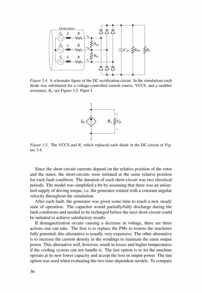
3.4.1 Electrical circuitThe electrical circuit consisted of a full wave three phase diode rectifyingbridge connected to the generator output with a resistive load (RL) and a ca-pacitor (CDC) on the DC side, as shown in Figure 3.4. The capacitor was addedto lower the voltage ripple. Ea, Eb, Ec are the generator electromotive forcesand va, vb, vc are the generator output line-neutral voltages of phase a, b and c,respectively. L and R are the generator inductance and the internal resistanceper phase, respectively. Further, there are three resistors denoted Rab, Rbc, andRDC which were used as switches in the short-circuit simulations. The com-ponents in the generator block of Figure 3.4 were not included in the circuit

34

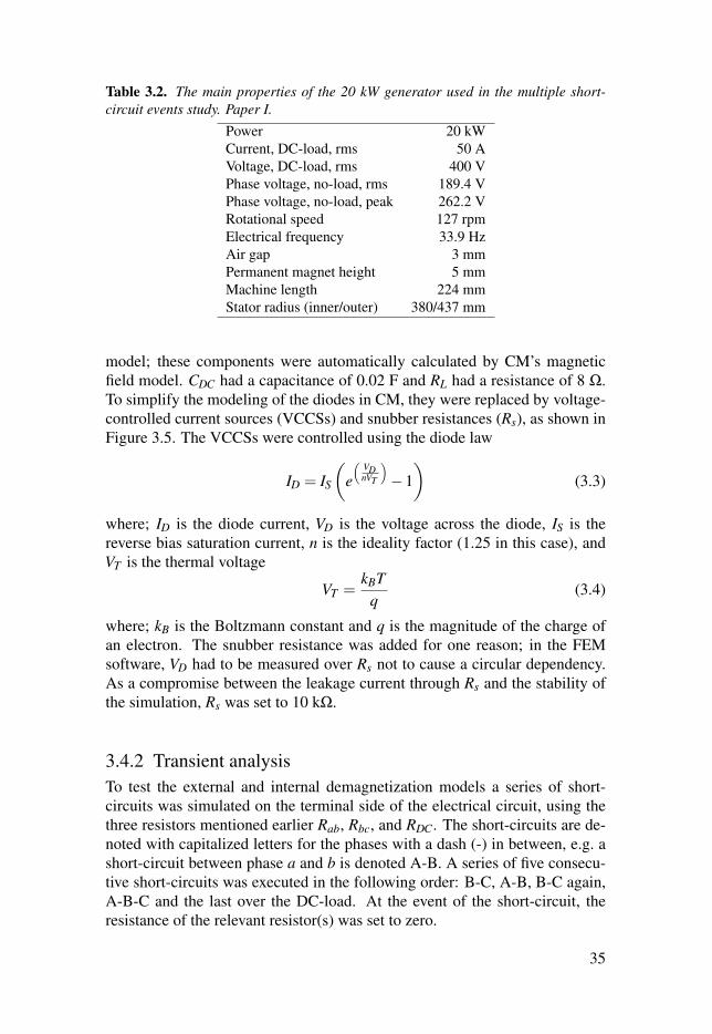
Table 3.2. The main properties of the 20 kW generator used in the multiple short-circuit events study. Paper I.

Power 20 kWCurrent, DC-load, rms 50 AVoltage, DC-load, rms 400 VPhase voltage, no-load, rms 189.4 VPhase voltage, no-load, peak 262.2 VRotational speed 127 rpmElectrical frequency 33.9 HzAir gap 3 mmPermanent magnet height 5 mmMachine length 224 mmStator radius (inner/outer) 380/437 mm

model; these components were automatically calculated by CM’s magneticfield model. CDC had a capacitance of 0.02 F and RL had a resistance of 8 Ω.To simplify the modeling of the diodes in CM, they were replaced by voltage-controlled current sources (VCCSs) and snubber resistances (Rs), as shown inFigure 3.5. The VCCSs were controlled using the diode law

ID = IS

(e(

VDnVT

)−1

)(3.3)

where; ID is the diode current, VD is the voltage across the diode, IS is thereverse bias saturation current, n is the ideality factor (1.25 in this case), andVT is the thermal voltage

VT =kBT

q(3.4)

where; kB is the Boltzmann constant and q is the magnitude of the charge ofan electron. The snubber resistance was added for one reason; in the FEMsoftware, VD had to be measured over Rs not to cause a circular dependency.As a compromise between the leakage current through Rs and the stability ofthe simulation, Rs was set to 10 kΩ.

3.4.2 Transient analysisTo test the external and internal demagnetization models a series of short-circuits was simulated on the terminal side of the electrical circuit, using thethree resistors mentioned earlier Rab, Rbc, and RDC. The short-circuits are de-noted with capitalized letters for the phases with a dash (-) in between, e.g. ashort-circuit between phase a and b is denoted A-B. A series of five consecu-tive short-circuits was executed in the following order: B-C, A-B, B-C again,A-B-C and the last over the DC-load. At the event of the short-circuit, theresistance of the relevant resistor(s) was set to zero.

35

Generator

RLCdc RDC

Ea L Rva

Eb L R Rabvb

Ec L R Rbcvc

Figure 3.4. A schematic figure of the DC rectification circuit. In the simulations eachdiode was substituted for a voltage-controlled current source, VCCS, and a snubberresistance, Rs, see Figure 3.5. Paper I.

ID Rs

+

−VD

Figure 3.5. The VCCS and Rs which replaced each diode in the DC-circuit of Fig-ure 3.4.

Since the short-circuit currents depend on the relative position of the rotorand the stator, the short-circuits were initiated at the same relative positionfor each fault condition. The duration of each short-circuit was two electricalperiods. The model was simplified a bit by assuming that there was an unlim-ited supply of driving torque, i.e. the generator rotated with a constant angularvelocity throughout the simulation.

After each fault, the generator was given some time to reach a new steadystate of operation. The capacitor would partially/fully discharge during thefault conditions and needed to be recharged before the next short-circuit couldbe initiated to achieve satisfactory results.

If demagnetization occurs causing a decrease in voltage, there are threeactions one can take. The first is to replace the PMs to restore the machinesfully potential, this alternative is usually very expensive. The other alternativeis to increase the current density in the windings to maintain the same outputpower. This alternative will, however, result in losses and higher temperaturesif the cooling system can not handle it. The last option is to let the machineoperate at its new lower capacity and accept the loss in output power. The lastoption was used when evaluating the two time-dependent models. To compare

36

the severity of the different short-circuit events, all cases were also tested on ahealthy machine.

3.4.3 Comparison with stationary modelTo further evaluate the models, they were compared to the stationary modelwhich was verified with experiments in Paper IV and Section 3.3. The com-parison was performed in a three-legged iron core, where the middle leg had a1 mm air gap separating a permanent magnet and a coil of 100 turns. The am-bient temperature was set to 20C. A series of current pulses with a maximumpeak value of 60 A and a duration of 1 s was led through the coil.

3.5 Ripple in surface mounted permanent magnetsWhen passively rectifying a generator output voltage using diodes, there areharmonics introduced into the current. These current fluctuations will in theirturn cause a ripple in the magnetic field. Therefore, the PMs of a PMSG willbe subjected to different magnetic loading depending not only on the electricalloading but also the type of electrical system the generator is connected to. Thedifference in working point and in particular the ripple of the working pointfor the PMs in a PMSG was studied in Paper II, for three different load cases;no-load, a purely resistive Y-connected alternating current (AC)-load, and adiode rectified DC-load (the same circuit as in Figure 3.4). The magnetic fluxdensity was recorded in three positions close to the surface of the PM, shownin Figure 3.6. The average magnetic flux density of the PM was also recorded.The generator in this study was a 100 kW generic modification of the 12 kWPMSG lab generator. The loads in the different load cases were adjusted untilthe same output power of 100±0.1 kW was achieved from the generator. Formore details about the study, please refer to Paper II.

3.6 Comparison of ferrite and Nd-Fe-B rotorIn the aftermath of the sudden Nd-Fe-B PM price peak at the end of 2011 andthe growing debate about the environmental impact of the mining for the rareearth metals [53, 54] used in Nd-Fe-B PMs, the idea of building a generatorwith an interchangeable rotor took form [55]. The main idea was to be ableto have a generator with as similar properties as possible with both a Nd-Fe-B and a ferrite rotor, and depending on the current price levels buildingthe most profitable one. There are some challenges with this; ferrites haveapproximately one-third of the remanence and about one-tenth of the energyproduct compared to Nd-Fe-B PMs. Therefore, about ten times more PM-material is needed to generate the same magnetic flux density in the air gap.

37

A

B

C

Figure 3.6. Cross section of one-fourth of the geometry simulated in Paper II. The

positions A, B, and C are positioned along a line 1 mm below the surface of the

magnet. A and B are each 1 mm from the respective side, and B is placed in the

middle of the permanent magnet. The rotational direction of the rotor is clockwise.

The 12 kW generator in Paper V was used as a reference to the new ferrite

rotor generator and is further described in [56, 57]. The design procedure of

the ferrite rotor is described in Paper VI.

To further analyse and compare the two generators, the short-circuit behav-

ior and demagnetization risk under different conditions were analysed for the

two generators. Since the mass and the mass moment of inertia are very differ-

ent for the two machines, the short-circuit simulations were also modified to

include the influence of the mass moment of inertia. To expand the study even

further, the mass moment of inertia of a wind turbine was introduced into the

problem to compare how the generators behaved when connected to a wind

turbine and when the turbine was not considered.

38

4. Summary of results and discussion

4.1 Experimental verificationThe results of the experimental verification study were overall satisfactory de-spite some troubles with the PM samples and the set-up, as discussed below.The results in this section are based on a total of three PM samples. Mea-surement and simulation results from two samples are plotted in Figure 4.1.The maximum deviation of B|| in the simulation results compared to the ex-perimental results before demagnetization was 7.9%. After demagnetizationthe same number was 17.8%. However, neglecting the two outer points themaximum deviation between simulations and experiments drops down to 3%.The cause for the bigger deviation of the results close to the edge could be aconsequence of the model only considering the magnetic flux parallel to themagnetization direction. Figure 4.2 shows an example of the resolution thatcould be achieved in the demagnetization simulations. The figure shows, anexample of, the demagnetization after a phase to phase short-circuit in the12 kW PMSG studied in Paper V.

The results are only based three samples due to the poor sample quality.During calibration of the PMs, it was discovered that the PMs differed verymuch in quality. Some samples had very low Br, and some were not evenly

0 10 20 30 40 500

0.2

0.4

0.6

0.8

1

Position (mm)0 10 20 30 40 50

0

0.2

0.4

0.6

0.8

1

Position (mm)

Mag

netic

flux

dens

ity(T

)

Sim. before Sim. after Exp. before Exp. after

Figure 4.1. The magnetic flux density as a function of the position in the PMs for twosamples. Paper IV.

39

100

70

80

90

%o

fB

r

Figure 4.2. Example of the resolution of the demagnetization in a permanent magnet.

The generator in the figure is the 12 kW machine studied in Paper V.

magnetized. Therefore, the decision was made to only include the PMs with a

rather high and even magnetization. The values of Hc and HcJ was not within

the limits of Table 3.1. It seemed that the percentage difference for the Br was

about the same as for Hc and HcJ compared to the calibrated sample. During

the experiments it was therefore assumed that the percentage difference of Brcompared to the calibrated sample was of the same size for Hc and HcJ , i.e.

if Br was 5% lower than the calibrated sample the values of Hc and HcJ were

assumed to be 5% lower as well.

Iron core measurementsWhile analyzing and measuring the iron core properties, the experimental re-

sults did not coincide with the simulated results. The simulation results under-

estimated B at low currents and overestimated B at high currents. Due to these

results, some leftover pieces of the iron core material were control measured

at the manufacturer using an Epstein frame. Using the resulting B-H-curve

from that measurement in the simulations improved the results, but they were

still not perfect.

The non-perfect correlation between the simulated and experimental results

could be caused by the orientation of the steel’s rolling direction (RD) in the

experimental set-up. Steel has different properties in the RD, and the trans-

verse direction (TD) and the magnetic properties are usually better in the RD.

When measuring in an Epstein frame equal number of steel pieces oriented in

the RD and the TD are used. Measurements, therefore, result in a B-H-curve

which corresponds to an average of the two directions. In the experimental

set-up the RD was in the horizontal direction of Figure 3.2, i.e. the magnetic

field has to travel further in the TD than in the RD. At the same time, the

magnetic field in RD parts would be higher than what the simulation results

40

show. The effect of the rolling direction orientation could explain a part of thedeviation between the simulated and experimental results.

4.2 Time-dependent modelsResults from the transient analysis of the two time-dependent demagnetiza-tion models showed that the power output decreased from the original 20 kWto 13.5 kW and 13.1 kW due to the demagnetization, for the external and inter-nal model respectively. The capacitor voltage, which is directly proportionalto the current in the resistive load and hence the delivered power, is plottedin Figure 4.3. The major part of the demagnetization occurred during the twofirst short-circuits. There is a slight voltage drop not visible in Figure 4.3 inthe second to last fault condition, the A-B-C short-circuit. It can also be seenin Figure 4.3 that the generator was allowed to reach a new steady state ofoperation before each fault condition, as discussed earlier. The reason for theinitial increase in capacitor voltage is because the initial value of the capacitorvoltage in the simulation was set to 360 V. A more detailed plot over the short-circuit consequences is plotted in Figure 4.4, where the average Br in all fourPMs is shown. The smallest repeatable part of this generator was of two polepairs, and the geometry was similar to the one in Figure 2.3 in Section 2.2.With the PMs denoted 1 to 4 from the bottom up. The series of short-circuitevents resulted in an unsymmetrical demagnetization of the PMs as shown inFigure 4.4. It can be noticed that the average Br is only slightly decreased(0.8%) in PM 1 while PM 3 experienced a decline of 23.8% in average Br.The unsymmetrical demagnetization can also be observed when comparingthe no-load voltage before and after the short-circuit events, which are plottedin Figure 4.5. The unsymmetrical no-load voltage is a direct cause of theunsymmetrical demagnetization of the PMs. This uneven induced voltage willalso have an influence on the torque. While performing a frequency analysisof the no-load voltage, an overtone with a frequency of 1.5 fel was found whichis directly coupled to the torque ripple. An increase in torque ripple could leadto increased vibrations which in turn could result in problems, especially atlower frequencies when there is less damping by the generator and shaft dy-namics. Low vibrational frequencies can, therefore, more easily transfer to theturbine from the shaft of the generator [58]. As mentioned above, the majorityof the demagnetization occurred during the first two short-circuit events. Ifthe current had been adjusted to maintain the output power, the short-circuitcurrent would have been higher in the later cases leading to higher demagne-tization in the end. Since the load was kept constant, the current reduced as aconsequence of the decreased induced voltage. The no-load voltage after thefinal demagnetization was 156 V for the external model. This voltage levelis close to the no-load voltage after the worst case on a healthy machine, theA-B-C fault. The no-load voltage after an A-B-C case on a healthy machine

41

0 100 200 300 400 500 600 700 800 900 10000

100

200

300

400

500

Time (ms)

Volta

ge(V

)Int modelExt model

Figure 4.3. Voltage over the capacitor during all the successive fault events for bothmodels. Paper I.

0 100 200 300 400 500 600 700 800 900 10000.9

1

1.1

1.2

1.3

Time (ms)

Ave

rage

rem

anen

ce(T

) PM 1PM 2PM 3PM 4

Figure 4.4. The average remanence in each magnet during all short-circuit events forthe external model. Adapted from Paper I.

was 154 V. This suggests that it is not the number of fault conditions thatdetermines the damage on a machine, but which cases it is exposed too.

Comparing the two time-dependent demagnetization models to the station-ary model shows that the computational time of the external model is aboutfour times longer than for the internal model. However, the internal modeltends to overestimate the demagnetization slightly. For detailed results re-garding the comparison with the stationary model, please refer to Paper I,more specifically Table 3.

42

0 10 20 30 40 50 60−300

−200

−100

0

100

200

300Vo

ltage

(V)

vavbvc

Figure 4.5. The no-load voltage for the 20 kW generator, before (solid) and after(dashed) the short-circuit events for the external model. Adapted from Paper I.

4.3 Ripple in permanent magnetsResults from the FEM simulations showed a small difference in working pointbetween the different load cases, the largest difference was at the corners. Inthe no-load case the amplitude of the magnetic flux density at position A andC were almost the same, as expected. When loading the generator the trailingcorner, A in this case, will experience a rise in the magnetic flux density whilethe leading corner, C, will experience a decrease in magnetic flux density. Theripple of the magnetic flux density at the different positions during the differentload cases is presented in Figure 4.6.

A frequency analysis of the results in Figure 4.6 revealed that the slot har-monic at 7.5 fel was present in all loading conditions, but mainly at the surfaceof the PM. An unexpected harmonic at 1.5 fel occurred, which did not seem toarise from any harmonic in the electrical current, and was therefore assumedto be an undertone of the slot harmonics. Small harmonics at 3, 4.5 and (forthe AC-load case) 6 fel were also assumed to be a consequence of the slotting.

The 6 fel harmonic in the DC-load case was significantly higher than in theAC-load case. The 6 fel harmonic was caused by the current fluctuation duringthe passive rectification and can be significant. In the original 12 kW machine,the fluctuation in electric torque at nominal power was determined to be in therange of 20-30% [58]. The value obtained for this 100 kW machine was only6%, and the resulting magnetic field ripple was at most 1.54% for the studiedpositions. The reason for the low power fluctuation in the 100 kW machinewas the high current in combination with the large generator inductance.

43

0.60.70.80.9

11.1 AC

Mag

netic

flux

dens

ity(T

)

0 20 40 60 80 100 120 140 160 180 2000.60.70.80.9

11.1 DC

Time (ms)

0.60.70.80.9

11.1 No-load

A B C Avg.

Figure 4.6. The ripple of the average of the magnetic flux density, and in the differentpoints within the PM during no-load, AC-load, and DC-load at 60C. Paper II

4.4 The ferrite alternativeThe generator characteristics for the ferrite- and the Nd-Fe-B rotor generatorsare found in Table 4.1. The electrical properties are somewhat different sincethe induced voltage of the ferrite rotor generator was lower, therefore, thearmature current had to be increased to maintain the same output power. In thiscase, this was not a problem since the armature current density was rather lowand increasing it would not dramatically increase the current losses. On thepositive side, the iron losses decreased as a consequence of the lower magneticflux density of the ferrite rotor. However, the overall electromagnetic losseswere slightly increased. Further, due to the use of ferrite PMs, the total massof the rotor has been increased by more than three times. This increase is notonly due to the increased weight of the PMs but also due to the weight of thepole shoes and the extra support structure needed.

The basic electrical and mechanical properties of the ferrite rotor design israther similar to the Nd-Fe-B design. One big reason for the induced volt-age not decreasing more was that the air gap width was decreased from 10 to

44

Table 4.1. A comparison of the generator characteristics for the old Nd-Fe-B and newferrite design. Values are at rated load and speed. All values are from simulationsexcept for the weights of the old design. Paper VI

Quantity NdFeB rotor Ferrite rotorRated power 12 kW 12 kWPhase voltage, no load, rms 172 V 146 VPhase voltage, rms 167 V 141 VArmature current, rms 23.9 A 28.5 AArmature current density, rms 1.49 A/mm2 1.78 A/mm2

Amplitude of the fundamentalair gap flux density at no load 0.79 T 0.66 TResistive losses 275 W 390 WIron losses 254 W 159 WElectromagnetic efficiency 95.8% 95.6%Minimum air gap 10 mm 7 mmMass of rotor 130 kg 407 kgMass of PMs 41 kg 158 kgMoment of inertia 16.9 kgm2 34.2 kgm2

PM material grade N40 Y40Remanence of PMs 1.27 T 0.45 TMaximum energy product 310 kJ/m3 47.6 kJ/m3

7 mm. By doing this, the reluctance in the air gap decreased and in additionmore PM material could be fitted in the rotor. Since the Nd-Fe-B generatorwas used for educational and experimental purposes the design had not beenoptimized. Therefore, the same similarity of the electrical properties may bedifficult to achieve when converting other, already optimized, Nd-Fe-B ma-chines. Another criteria is that the machine must have a rather large rotorradius since so much ferrite PM material is required. The ferrite rotor has nowbeen built and has replaced the Nd-Fe-B rotor in the laboratory generator.

The results from the comparative study between the Nd-Fe-B and the fer-rite rotor generators showed that the Nd-Fe-B generator did not suffer fromdemagnetization, same as the results from Paper V. The ferrite rotor did sufferfrom demagnetization in all tested cases. However, although the minimum B||was well below the knee point, the induced no-load voltage only decreasedby <1% of all cases. As expected, the simulated short-circuit currents werehigher, and B|| was lower when the wind turbine was connected to the genera-tors.

Figure 4.7 shows the short-circuit currents for both generators during athree-phase-neutral fault. The short-circuit occurs after 7 ms, and the dis-tortion visible for the ferrite rotor is probably due to numerical errors duringthe simulation. It can be seen that the short-circuit currents are lower when thewind turbine is disconnected and that the rotational velocity of the Nd-Fe-B ro-tor has decreased significantly even in the short simulation span of Figure 4.7.

45

When the wind turbine is connected, the two generators behave similarly ex-cept that the current is higher in the Nd-Fe-B generator. In the simulations, thedriving torque on the wind turbine was assumed to be constant, i.e. the windturbine efficiency was independent of its rotational speed.

The reason the for the low induced voltage drop in the ferrite generator,although the minimum B|| was well below the knee point, is because of highbut local demagnetization of the ferrite PMs. The PMs were only damaged inthe corners which was somewhat expected due to the softer characteristics offerrite PMs as well as the high field concentration in the PM corners in a spoketype configuration.

-800

-400

0

400

800 NdFeB

Cur

rent

(A)

ia ib ic

0 10 20 30 40 50 60 70 80 90 100-800

-400

0

400

800 Ferrite

Time (ms)

Cur

rent

(A)

Figure 4.7. Currents for the Nd-Fe-B and ferrite generator during an A-B-C-N short-circuit. The solid and dashed lines are with and without turbine, respectively. Theshort-circuit occurred at 7 ms. Paper III

46

5. Conclusions

From the results presented in this thesis, it can be concluded that the demag-netization model works fairly well. The model has evolved throughout theproject and, in its latest form, the model is very easy to implement, only re-quiring a few steps to set-up in a new simulation model. However, with theconversion to use a DLL-file for the demagnetization model some featureswere left out, such as the exponential model and the temperature dependence.These features were left out due to the time limitation of the project, but can,however, easily be added again. The stationary model performed well in com-parison to experiments. Although the time-dependent model never was com-pared to experiments, the accuracy is expected to be similar to the stationarymodel since their working principle are the same.

A significant improvement of the simulation model was the implementa-tion of the electrical circuit. The model is capable of simulating the completeelectrical system of a machine.

The conversion from a Nd-Fe-B rotor to a ferrite rotor turned out well,achieving similar electrical properties in the new machine compared to theold. The induced voltage did, however, decrease somewhat due to a lower airgap magnetic flux density. By increasing the armature current, the same out-put power was maintained. The electromagnetic efficiency did only decreaseslightly due to this change.

The demagnetization comparison between the Nd-Fe-B and the ferrite ro-tor showed that the corners of the PMs in the ferrite would be demagnetizedduring the tested fault conditions. However, the induced voltage would onlydecrease less than 1%, according to the simulations. Results also confirmed alarge difference in short-circuit currents when a wind turbine was connectedto the generator, adding a significant amount of mass moment of inertia to thesystem. The Nd-Fe-B generator showed no sign of demagnetization during thesimulations with and without the connected wind turbine. It was also shown inPaper V that changing the mechanical design of the Nd-Fe-B generator wouldallow for the PM material to be reduced by more than 50%, maintain the sameelectrical properties, and still not risk demagnetization at a short-circuit fault.

From the study on multiple short-circuit events in Paper I the conclusionswere that even at low demagnetization and a low induced voltage drop, theinduced voltage can become unsymmetrical and potentially become a problemdue to higher amount of torque ripple. Further, it is the type of the short-circuit fault that determines the total demagnetization rather than the numberof short-circuit events. From this study, it was also concluded that the external

47

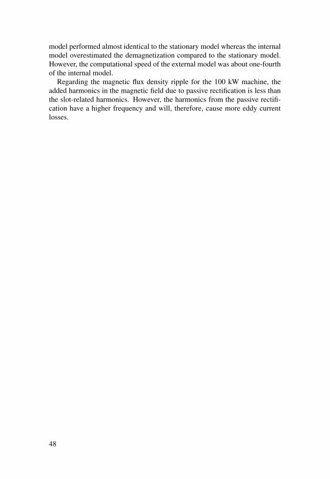
model performed almost identical to the stationary model whereas the internalmodel overestimated the demagnetization compared to the stationary model.However, the computational speed of the external model was about one-fourthof the internal model.

Regarding the magnetic flux density ripple for the 100 kW machine, theadded harmonics in the magnetic field due to passive rectification is less thanthe slot-related harmonics. However, the harmonics from the passive rectifi-cation have a higher frequency and will, therefore, cause more eddy currentlosses.

48

6. Summary of Papers

Paper IInvestigation of Permanent Magnet Demagnetization in Synchronous Ma-chines During Multiple Short-Circuit Fault Conditions

This paper compares the demagnetization characteristics of a PMSG withtwo different time-dependent demagnetization models developed in CM. Theferrite model is based on a proprietary external function, where the materialproperties are defined in an external C-file. The other internal model is basedon the ODE-module in CM. The results showed that the external model isabout four times slower but more accurate and more versatile than the internalmodel. Not only did the power output decrease by more than 30% after fivesuccessive faults but the no-load voltage had become unsymmetrical whichcould be explained by unsymmetrically demagnetized permanent magnets.The permanent magnet with the lowest decrease in average remanence haddecreased by 0.8% while the highest average reduction was 23.8% in anothermagnet.

The author did the majority of the work.The paper was submitted to IET Renewable Power Generation, September

2016.

Paper IIPermanent Magnet Working Point Ripple in Synchronous Generators

This article addresses the difference in working point and in particular themagnetic flux density ripple of the working point for the permanent magnetsin a PMSG. The working point ripple is studied for three different load cases;no-load, a purely resistive AC-load, and a diode-rectified DC-load. The re-sults show a smaller than expected difference in the working point, especiallybetween the AC and DC-load case. The frequency spectrum analysis of theaverage magnetic flux density inside a magnet showed an unexpected 1.5 felcomponent, assumed to be an undertone of the slot harmonic. Also, the addedharmonics in the magnetic field due to passive rectification is less than theslot-related harmonics.

The author contributed with the electromagnetic simulations and wrote mostof the paper.

The paper was submitted to IET Journal of Engineering, October 2016.

49

Paper IIIDetermining Demagnetisation Risk for Two PM Wind Power Generatorswith Different PM Material and Identical Stators

This paper evaluates the demagnetization risk of the 12 kW DDPMSG inPaper V compared to the demagnetization risk of the redesigned rotor from Pa-per VI during several different short-circuit events. In this study the torque andthe mass moment of inertia of the rotors and wind turbines were implementedto get more accurate results of the short-circuit currents. Results showed thatboth generators performed well. Both generators did suffer from a significantamount of demagnetization, but only when the operating temperature was wellout of normal operation intervals.

The author did the majority of the work.The paper was published in IET Electric Power Applications, August 2016,

doi:10.1049/iet-epa.2015.0518

Paper IVExperimental Verification of a Simulation Model for Partial Demagneti-zation of Permanent Magnets

This article aims to experimentally verify the simulation model first pre-sented in Paper V. Further development was made to the model since it wasoriginally presented. The main improvement was that a function of the mag-netic recoil behavior was added. To experimentally verify the simulationmodel an iron core with a coil capable of producing high magnetic field wasdesigned and built. The experimental set-up was modeled in the simulationsoftware and the experimental and simulation results were compared. Resultsshowed that the simulation model performed well and can predict demagne-tization behavior accurately. The simulations and experiments gave similarresults for most parts of the magnet.

The author did the majority of the work.The paper was published in IEEE Transactions on Magnetics, December

2014, doi:10.1109/TMAG.2014.2339795

Paper VStudy of Demagnetization Risk for a 12 kW Direct Driven PermanentMagnet Synchronous Generator for Wind Power

In this paper, the first version of the simulation model analyzing demagneti-zation of permanent magnets is presented. The paper consists of a simulation-based study of the use of different, cheaper, permanent magnet grades in a12 kW DDPMSG designed and constructed by the research group. Further,

50

an alternative geometry was suggested to study if less permanent magnet ma-terial could be used without the risk of demagnetization. Results showed thatthe only magnet grade that was not demagnetized during any of the assumedcases for both geometries was the one used in the built generator.

The author did the majority of the work.The paper was published in Energy Science & Engineering, December

2013, doi:10.1002/ese3.16.

Paper VIA Complete Design of a Rare Earth Metal-Free Permanent Magnet Gen-erator

This paper addresses the redesign of the rotor for a 12 kW DDPMSG. Themain objective was to design a completely new rotor with ferrite permanentmagnets replacing a rotor with Nd-Fe-B. The design includes both electro-magnetic and mechanic design, and the electromagnetic properties should beas close to the old design as possible. An entirely new design of a rotor withferrite magnets was presented. Simulations show comparable results to the olddesign even though the air gap magnetic flux density was reduced. To keepthe same output power the current needs to be increased slightly.

The author was a supervisor of the master thesis the paper was based onand was involved in the planning, execution of the project and writing of thepaper.

The paper was published in Machines, May 2014,doi:10.3390/machines2020120

51

7. Svensk sammanfattning

För att säkerställa att en permanentmagnetiserad generator kan leverera dessmärkeffekt genom hela dess livslängd krävs framförallt ett noggrant utfört des-ignarbete samt en god underhållsplan. Oavsett hur bra designad en maskin ärså kommer den förr eller senare behöva underhåll på ett eller annat sätt. De-signbiten är en smått delikat uppgift, dels behöver maskinen rent fysiskt klaraav de på frestningar som den kommer att utsättas för, samtidigt får maskineninte bli för dyr så att den inte blir lönsam. För den strukturmekaniska delenfinns det, i alla fall inom vissa användningsområden, riktlinjer och bestäm-melser för vilka säkerhetsmarginaler som krävs för den mekaniska konstruk-tionen. Den elektromagnetiska delen handlar framförallt om att optimera ut-nyttjandet av materialet på ett så bra sätt som möjligt. Det aktiva materialet ien generator, d.v.s. det järn som leder det magnetiska flödet samt permanent-magneterna, är en betydande del av kostnaden av maskinen. För järnet, ellerelektroplåt som det kallas, gäller det att optimera priset för materialet mot deförluster som kommer att uppstå i plåten. Bättre material med lägre förlusterkostar mer. Vad gäller valet av permanentmagneter är det inte lika självklart.Dels vill man att permanentmagneterna som levererar det magnetiska flödetska vara så starka som möjligt. Med starkare fält så ökar den inducerade spän-ningen i maskinen och en högre uteffekt kan erhållas. Däremot, klarar intestarka magneter så bra av motriktade fält eller höga temperaturer Detta kanleda till att magneterna kommer att avta i styrka d.v.s. avmagnetiseras. Detfinns givetvis magneter som kan utsättas för höga motriktade magnetiska fältutan att avmagnetiseras, dock så kommer detta att ske på bekostnad av att desjälva inte kommer kunna skapa ett lika starkt magnetiskt fält. Här måste manvälja om man vill vara säker på att magneterna kommer bibehålla sin styrkaäven efter eventuella felfall av höga motriktade magnetfält eller designa förstarkare magneter och hoppas på att underhållsarbetet kommer skydda mot deallvarligaste fel som skulle kunna skada magneterna.

Arbetet i denna doktorsavhandling behandlar framförallt avmagnetiseringav permanentmagneter samt simuleringar av olika typer av kortslutningsfelfall.En simuleringsmodell har utvecklats för detta ändamål. Tanken med dennasimuleringsmodell är att den ska kunna fungera som ett designverktyg för attutvärdera hur olika permanentmagnets kvalitéer fungerar i en viss maskin ochpå så sätt kunna välja en magnet som man tycker är lämplig. Avmagnetiser-ingsmodellen har, med goda resultat, jämförts med experiment som visat påliknande nivåer av avmagnetisering. Specifika studier där modellen har an-vänds har också genomförts däribland en jämförande studie där en rotor med

52

ytmonterade Neodym-Järn-Bor (Nd-Fe-B) magneter jämfördes med en rotormed ferritmagneter i ekerkonfiguration. Den studien var en del av en störrestudie där man ville undersöka huruvida det går att byta mellan de två ovannämnda rotortyperna och samtidigt bibehålla de elektriska egenskaperna hosmaskinen. Resultaten visade att man relativt bra kunde bibehålla de elektriskaegenskaperna för den specifika maskin som undersöktes i detta fall. Risken föravmagnetisering för de olika maskinerna var också snarlika. Även om rotornmed ferritmagneter avmagnetiserades i alla testade fall sjönk den induceradespänningen, enligt simuleringarna, med mindre än 1%.

Ett betydande steg i utvecklingen av avmagnetiseringsmodellen togs underdet senaste året då modellen gjordes om från grunden för att numera även varatidsberoende. Denna förändring tillsammans med utvecklingen av hur denelektriska kretsen till maskinerna simulerades resulterade i att multipla felfallnu kan studeras. Detta är viktigt då elektriska maskiner riskerar att utsättas förflera felfall under sin livstid och det är då viktigt att kunna förutse hur mask-inen kommer att bete sig. Resultatet från en sådan studie med fem varteftervarandra följande kortslutningar visade, inte helt överraskande, att det inteär antalet felfall som nödvändigtvis bestämmer hur mycket permanentmag-neterna skadas. Utan vilken typ av fel som uppstår. Denna studie visade ävenatt avmagnetiseringen i magneterna inte behöver vara jämn eller symmetrisktfördelad i magneterna. Denna asymmetri kommer ge upphov till övertoner ibåde inducerad spänning och uteffekt. Vidare så kan denna asymmetri ge cyk-liska krafter på rotorn vilket i längden skulle kunna leda till att till exempelkullager kommer att nötas ut snabbare än förutspått.

53

8. Acknowledgements

First, I would particularly like to express gratitude to my supervisor SandraEriksson for giving me this opportunity. Thank you for your patient and greatguidance during these years.

All my colleagues, past, and present, you have helped make work a fun placeto be. Special thanks to Mikael and Mårten for emphasizing that it is alwaysfive o’clock somewhere.

To all my roommates over these past years, thank you for all the laughs,time wasted on vaguely work-related discussions and your excellent bakingskills!

My Mom and Dad, my brother Krister with family; Marie-Louise, Carl, andSvea, thank you for everything.

Odd and Eva, I could not ask for better parents-in-law.I am also especially grateful to my lovely wife for always being there for

me. Our wonderful daughter Anna, you can brighten my day like no other. Ilove you both!

If I have forgotten anyone, please feel free to include yourself!

Finally, I would like to thank my financiers. This project has been supportedby the Swedish Research Council (grant number 2010-3950), StandUp for En-ergy and Uppsala University.

54

References

[1] J. Gieras and M. Wing, Permanent magnet motor technology: Design andapplications, 2nd ed. Boca Raton, FL, USA: Taylor & Francis, 2002.

[2] Y. Chen, P. Pillay, and A. Khan, “PM wind generator topologies,” IEEETransactions on Industry Applications, vol. 41, no. 6, pp. 1619–1626, Nov 2005.

[3] D. Trumper, W. jong Kim, and M. Williams, “Design and analysis frameworkfor linear permanent-magnet machines,” IEEE Transactions on IndustryApplications, vol. 32, no. 2, pp. 371–379, 1996.

[4] T.-F. Chan and L.-L. Lai, “Permanent-magnet machines for distributed powergeneration: A review,” in IEEE Power Engineering Society General Meeting,2007, Tampa, USA, June 2007, pp. 1–6.

[5] S. Hlioui, L. Vido, Y. Amara, M. Gabsi, M. Lecrivain, and A. Miraoui, “PM andhybrid excitation synchronous machines: Performances comparison,” in 18thInternational Conference on Electrical Machines (ICEM) 2008, Vilamoura,Portugal, September 2008, pp. 1–6.

[6] A. Kiyoumarsi, “Analysis and comparison of a permanent-magnet DC motorwith a field-winding DC motor,” Journal of Electrical Engineering &Technology, vol. 4, no. 3, pp. 370–376, September 2009.

[7] M. Hedlund, J. Lundin, J. de Santiago, J. Abrahamsson, and H. Bernhoff,“Flywheel energy storage for automotive applications,” Energies, vol. 8, no. 10,pp. 10 636–10 663, 2015.

[8] J. J. Croat, “High energy product rare earth-iron magnet alloys,” 1989, USPatent 4,851,058.

[9] O. Gutfleisch, M. A. Willard, E. Brück, C. H. Chen, S. G. Sankar, and J. P. Liu,“Magnetic materials and devices for the 21st century: Stronger, lighter, andmore energy efficient,” Advanced materials, vol. 23, pp. 821–842, 2011.

[10] J. Liu, T. Ohkubo, K. Hioki, A. Hattori, T. Schrefl, and K. Hono, “Effect of Ndcontent on the microstructure and coercivity of hot-deformed Nd-Fe-Bpermanent magnets,” Acta Materialia, vol. 61, pp. 5387–5399, June 2013.

[11] H. Sepehri-Amin, J. Liu, T. Ohkubo, K. Hioki, A. Hattori, and K. Hono,“Enhancement of coercivity of hot-deformed Nd-Fe-B anisotropic magnet bylow-temperature grain boundary diffusion of Nd-Dy-Cu eutectic alloy,” ScriptaMaterialia, vol. 69, pp. 647–650, July 2013.

[12] W. T. Thomson and M. Fenger, “Current signature analysis to detect inductionmotor faults,” IEEE Industry Applications Magazine, vol. 7, no. 4, pp. 26–34,July 2001.

[13] G. Singh and S. A. S. A. Kazzaz, “Induction machine drive conditionmonitoring and diagnostic research—a survey,” Electric Power SystemsResearch, vol. 64, no. 2, pp. 145 – 158, 2003.

[14] P. J. Tavnet, G. J. W. V. Bussel, and F. Spinato, “Machine and converterreliabilities in wind turbines,” in The 3rd IET International Conference on

55

Power Electronics Machines and Drives 2006, Dublin, Ireland, April 2006, pp.127–130.

[15] P. J. Tavner, “Review of condition monitoring of rotating electrical machines,”IET Electric Power Applications, vol. 2, no. 4, pp. 215–247, July 2008.

[16] J. A. Rosero, J. Cusido, A. Garcia, J. A. Ortega, and L. Romeral, “Study on thepermanent magnet demagnetization fault in permanent magnet synchronousmachines,” in IECON 2006 - 32nd Annual Conference on IEEE IndustrialElectronics, Paris, France, November 2006, pp. 879–884.

[17] D. Casadei, F. Filippetti, C. Rossi, and A. Stefani, “Magnets faultscharacterization for permanent magnet synchronous motors,” in IEEEInternational Symposium on Diagnostics for Electric Machines, PowerElectronics and Drives, 2009. SDEMPED 2009, Cargèse, France, August 2009,pp. 1–6.

[18] S. Chakraborty, E. Keller, A. Ray, and J. Mayer, “Detection and estimation ofdemagnetization faults in permanent magnet synchronous motors,” ElectricPower Systems Research, vol. 96, pp. 225 – 236, 2013.

[19] S. Ruoho, J. Kolehmainen, J. Ikäheimo, and A. Arkkio, “Interdependence ofdemagnetization, loading, and temperature rise in a permanent-magnetsynchronous motor,” IEEE Transactions on Magnetics, vol. 46, pp. 949–953,April 2010.

[20] C. Ruschetti, C. Verucchi, G. Bossio, C. D. Angelo, and G. García, “Rotordemagnetization effects on permanent magnet synchronous machines,” EnergyConversion and Management, vol. 74, pp. 1–8, October 2013.

[21] J. D. McFarland and T. M. Jahns, “Investigation of the rotor demagnetizationcharacteristics of interior PM synchronous machines during fault conditions,”IEEE Transactions on Industry Applications, vol. 50, no. 4, pp. 2768–2775, July2014.

[22] D. Givord, P. Tenaud, and T. Viadieu, “Angular dependence of coercivity insintered magnets,” Journal of Magnetism and Magnetic Materials, vol. 72,no. 3, pp. 247 – 252, 1988.

[23] G. Martinek and H. Kronmüller, “Influence of grain orientation of the coercivefield in Fe-Nd-B permanent magnets,” Journal of Magnetism and MagneticMaterials, vol. 86, no. 2, pp. 177 – 183, 1990.

[24] D. Plusa, “Angular dependence of coercivity in sintered NdDyFeB permanentmagnets,” Journal of Magnetism and Magnetic Materials, vol. 140, pp. 1061 –1062, 1995.

[25] D. Plusa and B. Wyslocki, “Magnetization reversal processes in sinteredNdFeBNb magnets,” Journal of Magnetism and Magnetic Materials, vol. 157,pp. 338 – 339, 1996.

[26] W. Fernengel, A. Lehnert, M. Katter, W. Rodewald, and B. Wall, “Examinationof the degree of alignment in sintered NdFeB magnets by measurements of theremanent polarizations,” Journal of Magnetism and Magnetic Materials, vol.157, pp. 19 – 20, 1996.

[27] R. Gao, W. Li, C. Ji, D. Zhang, and J. Zhang, “Effects of the grain alignment onthe coercivity and its angular dependence for NdCoFeB permanent magnets,”Chinese Science Bulletin, vol. 43, no. 2, pp. 107–111, 1998.

[28] K. C. Kim, S. B. Lim, D. H. Koo, and J. Lee, “The shape design of permanent

56

magnet for permanent magnet synchronous motor considering partialdemagnetization,” IEEE Transactions on Magnetics, vol. 42, no. 10, pp.3485–3487, October 2006.

[29] K.-Y. Hwang, S.-B. Rhee, J.-S. Lee, and B.-I. Kwon, “Shape optimization ofrotor pole in spoke type permanent magnet motor for reducing partialdemagnetization effect and cogging torque,” in International Conference onElectrical Machines and Systems, 2007. ICEMS, Seoul, South Korea, October2007, pp. 955–960.

[30] K. C. Kim, K. Kim, H. J. Kim, and J. Lee, “Demagnetization analysis ofpermanent magnets according to rotor types of interior permanent magnetsynchronous motor,” IEEE Transactions on Magnetics, vol. 45, no. 6, pp.2799–2802, June 2009.

[31] G. Zhao, L. Tian, Q. Shen, and R. Tang, “Demagnetization analysis ofpermanent magnet synchronous machines under short circuit fault,” inAsia-Pacific Power and Energy Engineering Conference 2010, ChengDu,China, March 2010, pp. 1–4.

[32] M. Katter, “Angular dependence of the demagnetization stability of sinteredNd-Fe-B magnets,” IEEE Transactions on Magnetics, vol. 41, no. 10, pp.3853–3855, November 2005.

[33] S. Ruoho and A. Arkkio, “Partial demagnetization of permanent magnets inelectrical machines caused by an inclined field,” IEEE Transactions onMagnetics, vol. 44, no. 7, pp. 1773–1778, August 2008.

[34] S. Apelfröjd, S. Eriksson, and H. Bernhoff, “A review of research on large scalemodern vertical axis wind turbines at uppsala university,” Energies, vol. 9, no. 7,p. 570, 2016.

[35] S. Eriksson, “Direct driven generators for vertical axis wind turbines,” Ph.D.dissertation, Digital Comprehensive Summaries of Uppsala Dissertations fromthe Faculty of Science and Technology 547, ISSN 1651-6214, 2008.

[36] J. Kjellin, “Vertical axis wind turbines - Electrical system and experimentalresults,” Ph.D. dissertation, Digital Comprehensive Summaries of UppsalaDissertations from the Faculty of Science and Technology 981, ISSN1651-6214, 2012.

[37] F. Bülow, “A generators perspective on vertical axis wind turbines,” Ph.D.dissertation, Digital Comprehensive Summaries of Uppsala Dissertations fromthe Faculty of Science and Technology 1034, ISSN 1651-6214, 2013.

[38] P. Deglaire, “Analytical aerodynamic simulation tools for vertical axis windturbines,” Ph.D. dissertation, Digital Comprehensive Summaries of UppsalaDissertations from the Faculty of Science and Technology 774, ISSN1651-6214, 2010.

[39] A. Goude, “Fluid mechanics of vertical axis turbines: Simulations and modeldevelopment,” Ph.D. dissertation, Digital Comprehensive Summaries ofUppsala Dissertations from the Faculty of Science and Technology 998, ISSN1651-6214, 2012.

[40] E. Dyachuk, “Aerodynamics of vertical axis wind turbines - Development ofsimulation tools and experiments,” Ph.D. dissertation, Digital ComprehensiveSummaries of Uppsala Dissertations from the Faculty of Science andTechnology 1274, ISSN 1651-6214, 2015.

57

[41] E. Möllerström, “Vertical axis wind turbines - Tower dynamics and noise,”Licentiate thesis, Uppsala University, Department of Engineering Sciences,ISSN 0349-8352; 340-15L, 2015.

[42] P. Eklund, “Rare earth metal-free permanent magnet generators,” Licentiatethesis, Uppsala University, Department of Engineering Sciences, ISSN0349-8352; 348-16L, 2016.

[43] M. Rossander, “Blade force measurements and electrical torque ripple of avertical axis wind turbine,” Licentiate thesis, Uppsala University, Department ofEngineering Sciences, ISSN 0349-8352; 346-16L, 2016.

[44] J. Olauson, “Modeling wind power for grid integration studies,” Ph.D.dissertation, Digital Comprehensive Summaries of Uppsala Dissertations fromthe Faculty of Science and Technology 1428, ISSN 1651-6214, 2016.

[45] S. Apelfröjd, “Grid connection of permanent magnet generator based renewableenergy systems,” Ph.D. dissertation, Digital Comprehensive Summaries ofUppsala Dissertations from the Faculty of Science and Technology 1436, ISSN1651-6214, 2016.

[46] J. William D. Callister, Materials science and engineering an introduction,6th ed. New York, NY, USA: John Wiley & Sons, Inc., 2003.

[47] B. Cullity and C. Graham, Introduction to Magnetic Materials, 2nd ed.Piscataway, NJ, USA: John Wiley & Sons, Inc., 2009.

[48] D. Jiles, Introduction to magnetism and magnetic materials, 2nd ed. BocaRaton, FL, USA: Taylor & Francis, 1998.

[49] M. S. Walmer, C. H. Chen, and M. H. Walmer, “A new class of Sm-Tm magnetsfor operating temperatures up to 550C,” IEEE Transactions on Magnetics,vol. 36, no. 5, pp. 3376–3381, September 2000.

[50] S. Ruoho, E. Dlala, and A. Arkkio, “Comparison of demagnetization models forfinite-element analysis of permanent-magnet synchronous machines,” IEEETransactions on Magnetics, vol. 43, no. 11, pp. 3964–3968, December 2007.

[51] S. Hamidizadeh, N. Alatawneh, R. R. Chromik, and D. A. Lowther,“Comparison of different demagnetization models of permanent magnet inmachines for electric vehicle application,” IEEE Transactions on Magnetics,vol. 52, no. 5, pp. 1–4, May 2016.

[52] H. C. Lovatt and P. A. Watterson, “Energy stored in permanent magnets,” IEEETransactions on Magnetics, vol. 35, no. 1, pp. 505–507, January 1999.

[53] B. Sprecher, Y. Xiao, A. Walton, J. Speight, R. Harris, R. Kleijn, G. Visser, andG. J. Kramer, “Life cycle inventory of the production of rare earths and thesubsequent production of NdFeB rare earth permanent magnets,” EnvironmentalScience & Technology, vol. 48, no. 7, pp. 3951–3958, 2014.

[54] J. C. K. Lee and Z. Wen, “Rare earths from mines to metals: Comparingenvironmental impacts from China’s main production pathways,” Journal ofIndustrial Ecology, September 2016.

[55] S. Eriksson and H. Bernhoff, “Rotor design for PM generators reflecting theunstable neodymium price,” in XXth International Conference on ElectricalMachines (ICEM) 2012, Marseille, France, September 2012, pp. 1419–1423.

[56] S. Eriksson, A. Solum, M. Leijon, and H. Bernhoff, “Simulations andexperiments on a 12 kW direct driven PM synchronous generator for windpower,” Renewable Energy, vol. 33, no. 4, pp. 674–681, May 2008.

58

[57] S. Eriksson, H. Bernhoff, and M. Leijon, “FEM simulations and experiments ofdifferent loading conditions for a 12 kW direct driven PM synchronousgenerator for wind power,” International Journal of Emerging Electric PowerSystems, vol. 10, no. 1, February 2009.

[58] M. Rossander, A. Goude, and S. Eriksson, “Mechanical torque ripple from apassive diode rectifier in a 12 kW vertical axis wind turbine,” To appear in IEEETransactions on Energy Conversion.

59

Acta Universitatis UpsaliensisDigital Comprehensive Summaries of Uppsala Dissertationsfrom the Faculty of Science and Technology 1444

Editor: The Dean of the Faculty of Science and Technology

A doctoral dissertation from the Faculty of Science andTechnology, Uppsala University, is usually a summary of anumber of papers. A few copies of the complete dissertationare kept at major Swedish research libraries, while thesummary alone is distributed internationally throughthe series Digital Comprehensive Summaries of UppsalaDissertations from the Faculty of Science and Technology.(Prior to January, 2005, the series was published under thetitle “Comprehensive Summaries of Uppsala Dissertationsfrom the Faculty of Science and Technology”.)

Distribution: publications.uu.seurn:nbn:se:uu:diva-303517

ACTAUNIVERSITATIS

UPSALIENSISUPPSALA

2016