delta function, the fourier transform, and fourier integral theorem
TRANSCRIPT

Gauge Institute Journal, Volume 8, No.2, May 2012 H. Vic Dannon
Delta Function, the Fourier Transform,
and Fourier Integral Theorem H. Vic Dannon
[email protected] September, 2010
Abstract The Fourier Integral Theorem guarantees that the
Fourier Transform and its Inverse are well defined operations, so
that the inversed transform is the originally transformed function.
It is believed to hold in the Calculus of Limits under some highly
restrictive sufficient conditions. In fact,
The Theorem does not hold in the Calculus of Limits
under any conditions,
because evaluating the Fourier Integral requires the integration of
( )k
ik x
k
e dξ=∞
−
=−∞∫ k ,
that diverges at x . ξ=
Only in Infinitesimal Calculus, the integral is the Hyper-real
Delta Function
( )1( )
2
kik x
k
x e ξδ ξπ
=∞−
=−∞
− = ∫ dk ,
1
Gauge Institute Journal, Volume 8, No.2, May 2012 H. Vic Dannon
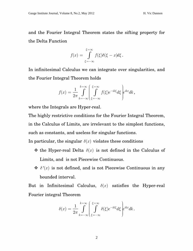
and the Fourier Integral Theorem states the sifting property for
the Delta Function
( ) ( ) ( )f x fξ
ξ
ξ δ ξ ξ=∞
=−∞
= −∫ x d .
In infinitesimal Calculus we can integrate over singularities, and
the Fourier Integral Theorem holds
1( ) ( )
2
kik ikx
k
f x f eξ
ξ
ξ
ξ ξπ
=∞ =∞−
=−∞ =−∞
⎛ ⎞⎟⎜ ⎟⎜ ⎟= ⎜ ⎟⎜ ⎟⎜ ⎟⎝ ⎠∫ ∫ d e dk ,
where the Integrals are Hyper-real.
The highly restrictive conditions for the Fourier Integral Theorem,
in the Calculus of Limits, are irrelevant to the simplest functions,
such as constants, and useless for singular functions.
In particular, the singular violates these conditions ( )xδ
the Hyper-real Delta is not defined in the Calculus of
Limits, and is not Piecewise Continuous.
( )xδ
is not defined, and is not Piecewise Continuous in any
bounded interval.
'( )xδ
But in Infinitesimal Calculus, satisfies the Hyper-real
Fourier integral Theorem
( )xδ
1( ) ( )
2
kik ikx
k
x eξ
ξ
ξ
δ δ ξπ
=∞ =∞−
=−∞ =−∞
⎛ ⎞⎟⎜ ⎟⎜ ⎟= ⎜ ⎟⎜ ⎟⎜ ⎟⎝ ⎠∫ ∫ d e dkξ .
2

Gauge Institute Journal, Volume 8, No.2, May 2012 H. Vic Dannon
Also, the constant function ( ) 1f x ≡ violates the sufficient
conditions’ requirement of absolute integrability, 1x
x
dx=∞
=−∞
= ∞∫ .
But in Infinitesimal Calculus, ( ) 1f x ≡ satisfies the Hyper-real
Fourier integral Theorem
11
2
kik ikx
k
e d e dξ
ξ
ξ
ξπ
=∞ =∞−
=−∞ =−∞
⎛ ⎞⎟⎜ ⎟⎜ ⎟= ⎜ ⎟⎜ ⎟⎜ ⎟⎝ ⎠∫ ∫ k .
Keywords: Infinitesimal, Infinite-Hyper-Real, Hyper-Real
Function, Infinitesimal Calculus, Delta Function, Fourier
Transform, Fourier Integral Theorem
2000 Mathematics Subject Classification 26E15; 26E20;
26A06; 97I40; 97I30; 44A10;
3
Gauge Institute Journal, Volume 8, No.2, May 2012 H. Vic Dannon
Contents
Introduction
1. Hyper-real Line
2. Integral of a Hyper-real Function
3. Delta Function
4. and the Fourier Transform ( )xδ
5. Fourier Integral Theorem
6. Cosine representation of and the Fourier integral ( )xδ
Theorem
7. and the Fourier Transform ( , )x yδ
8. and the Fourier transform ( , , )x y zδ
9. Delta Sequence 2
2
sin( )( )n
n nxx
nxδ
π
⎛ ⎞⎟⎜= ⎟⎜ ⎟⎟⎜⎝ ⎠
4

Gauge Institute Journal, Volume 8, No.2, May 2012 H. Vic Dannon
Introduction By Fourier Integral Theorem
1( ) ( )
2
kik ikx
k
f x f eξ
ξ
ξ
ξ ξπ
=∞ =∞−
=−∞ =−∞
⎛ ⎞⎟⎜ ⎟⎜ ⎟= ⎜ ⎟⎜ ⎟⎜ ⎟⎝ ⎠∫ ∫ d e dk
( )1( )
2
kik x
k
f e dkξ
ξ
ξ
ξ ξπ
=∞ =∞−
=−∞ =−∞
⎛ ⎞⎟⎜ ⎟⎜ ⎟= ⎜ ⎟⎜ ⎟⎜ ⎟⎝ ⎠∫ ∫ d
Thus, the integral ( )12
kik x
k
e ξ
π
=∞− −
=−∞∫ dk sifts through the values of
the function ( )f ξ , and picks its value at x .
Cauchy (1816), and Poisson (1815) derived the Fourier Integral
Theorem by using the sifting property of the integral.
In the derivation of his Zeta Function, Riemann (1859) uses this
sifting property repeatedly, without using a function notation for
the integral ( )12
kik x
k
e ξ
π
=∞− −
=−∞∫ dk . The derivations are in [Dan4,
p.84, p.90, p.97].
However, ( ) 1ik xx e ξξ − −= ⇒ = ,
and the integral ( )12
kik x
k
e ξ
π
=∞− −
=−∞∫ dk diverges.
5
Gauge Institute Journal, Volume 8, No.2, May 2012 H. Vic Dannon
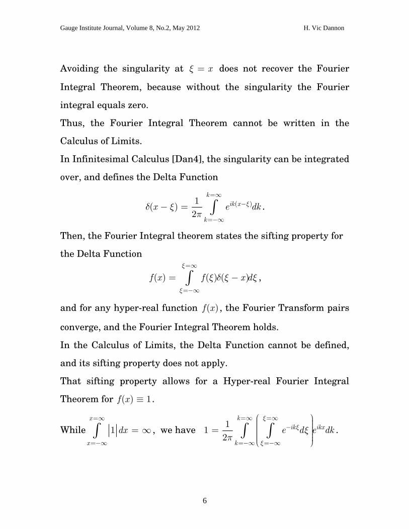
Avoiding the singularity at does not recover the Fourier
Integral Theorem, because without the singularity the Fourier
integral equals zero.
xξ =
Thus, the Fourier Integral Theorem cannot be written in the
Calculus of Limits.
In Infinitesimal Calculus [Dan4], the singularity can be integrated
over, and defines the Delta Function
( )1( )
2
kik x
k
x e ξδ ξπ
=∞−
=−∞
− = ∫ dk .
Then, the Fourier Integral theorem states the sifting property for
the Delta Function
( ) ( ) ( )f x fξ
ξ
ξ δ ξ ξ=∞
=−∞
= −∫ x d ,
and for any hyper-real function ( )f x , the Fourier Transform pairs
converge, and the Fourier Integral Theorem holds.
In the Calculus of Limits, the Delta Function cannot be defined,
and its sifting property does not apply.
That sifting property allows for a Hyper-real Fourier Integral
Theorem for ( ) 1f x ≡ .
While 1x
x
dx=∞
=−∞
= ∞∫ , we have 11
2
kik ikx
k
e d e dξ
ξ
ξ
ξπ
=∞ =∞−
=−∞ =−∞
⎛ ⎞⎟⎜ ⎟⎜ ⎟= ⎜ ⎟⎜ ⎟⎜ ⎟⎝ ⎠∫ ∫ k .
6

Gauge Institute Journal, Volume 8, No.2, May 2012 H. Vic Dannon
1.
Hyper-real Line Each real number α can be represented by a Cauchy sequence of
rational numbers, so that . 1 2 3( , , ,...)r r r nr α→
The constant sequence ( is a constant hyper-real. , , ,...)α α α
In [Dan2] we established that,
1. Any totally ordered set of positive, monotonically decreasing
to zero sequences constitutes a family of
infinitesimal hyper-reals.
1 2 3( , , ,...)ι ι ι
2. The infinitesimals are smaller than any real number, yet
strictly greater than zero.
3. Their reciprocals (1 2 3
1 1 1, , ,...ι ι ι ) are the infinite hyper-reals.
4. The infinite hyper-reals are greater than any real number,
yet strictly smaller than infinity.
5. The infinite hyper-reals with negative signs are smaller
than any real number, yet strictly greater than −∞ .
6. The sum of a real number with an infinitesimal is a
non-constant hyper-real.
7. The Hyper-reals are the totality of constant hyper-reals, a
family of infinitesimals, a family of infinitesimals with
7
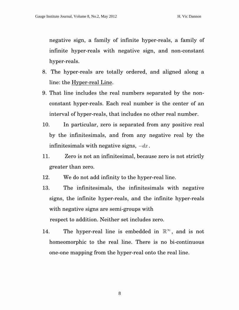
Gauge Institute Journal, Volume 8, No.2, May 2012 H. Vic Dannon
negative sign, a family of infinite hyper-reals, a family of
infinite hyper-reals with negative sign, and non-constant
hyper-reals.
8. The hyper-reals are totally ordered, and aligned along a
line: the Hyper-real Line.
9. That line includes the real numbers separated by the non-
constant hyper-reals. Each real number is the center of an
interval of hyper-reals, that includes no other real number.
10. In particular, zero is separated from any positive real
by the infinitesimals, and from any negative real by the
infinitesimals with negative signs, . dx−
11. Zero is not an infinitesimal, because zero is not strictly
greater than zero.
12. We do not add infinity to the hyper-real line.
13. The infinitesimals, the infinitesimals with negative
signs, the infinite hyper-reals, and the infinite hyper-reals
with negative signs are semi-groups with
respect to addition. Neither set includes zero.
14. The hyper-real line is embedded in , and is not
homeomorphic to the real line. There is no bi-continuous
one-one mapping from the hyper-real onto the real line.
∞
8

Gauge Institute Journal, Volume 8, No.2, May 2012 H. Vic Dannon
15. In particular, there are no points on the real line that
can be assigned uniquely to the infinitesimal hyper-reals, or
to the infinite hyper-reals, or to the non-constant hyper-
reals.
16. No neighbourhood of a hyper-real is homeomorphic to
an ball. Therefore, the hyper-real line is not a manifold. n
17. The hyper-real line is totally ordered like a line, but it
is not spanned by one element, and it is not one-dimensional.
9

Gauge Institute Journal, Volume 8, No.2, May 2012 H. Vic Dannon
2.
Integral of a Hyper-real Function
In [Dan3], we defined the integral of a Hyper-real Function.
Let ( )f x be a hyper-real function on the interval [ , . ]a b
The interval may not be bounded.
( )f x may take infinite hyper-real values, and need not be
bounded.
At each
a x≤ ≤ b ,
there is a rectangle with base 2
[ ,dx dxx x− +2], height ( )f x , and area
( )f x dx .
We form the Integration Sum of all the areas for the x ’s that
start at x , and end at x b , a= =
[ , ]
( )x a b
f x dx∈∑ .
If for any infinitesimal dx , the Integration Sum has the same
hyper-real value, then ( )f x is integrable over the interval [ , . ]a b
Then, we call the Integration Sum the integral of ( )f x from ,
to x , and denote it by
x a=
b=
10

Gauge Institute Journal, Volume 8, No.2, May 2012 H. Vic Dannon
( )x b
x a
f x dx=
=∫ .
If the hyper-real is infinite, then it is the integral over [ , , ]a b
If the hyper-real is finite,
( ) real part of the hyper-realx b
x a
f x dx=
=
=∫ .
2.1 The countability of the Integration Sum
In [Dan1], we established the equality of all positive infinities:
We proved that the number of the Natural Numbers,
Card , equals the number of Real Numbers, , and
we have
2CardCard =
2 2( ) .... 2 2 ...CardCardCard Card= = = = = ≡ ∞ .
In particular, we demonstrated that the real numbers may be
well-ordered.
Consequently, there are countably many real numbers in the
interval [ , , and the Integration Sum has countably many terms. ]a b
While we do not sequence the real numbers in the interval, the
summation takes place over countably many ( )f x dx .
11

Gauge Institute Journal, Volume 8, No.2, May 2012 H. Vic Dannon
The Lower Integral is the Integration Sum where ( )f x is replaced
by its lowest value on each interval 2 2
[ ,dx dxx x− + ]
2.2 2 2[ , ]
inf ( )dx dxx t xx a b
f t dx− ≤ ≤ +∈
⎛ ⎞⎟⎜ ⎟⎜ ⎟⎜ ⎟⎜⎝ ⎠∑
The Upper Integral is the Integration Sum where ( )f x is replaced
by its largest value on each interval 2 2
[ ,dx dxx x− + ]
2.3 2 2[ , ]
sup ( )dx dxx t xx a b
f t dx− ≤ ≤ +∈
⎛ ⎞⎟⎜ ⎟⎜ ⎟⎜ ⎟⎜ ⎟⎝ ⎠∑
If the integral is a finite hyper-real, we have
2.4 A hyper-real function has a finite integral if and only if its
upper integral and its lower integral are finite, and differ by an
infinitesimal.
12

Gauge Institute Journal, Volume 8, No.2, May 2012 H. Vic Dannon
3.
Delta Function In [Dan5], we have defined the Delta Function, and established its
properties
1. The Delta Function is a hyper-real function defined from the
hyper-real line into the set of two hyper-reals 1
0,dx
⎧ ⎫⎪⎪⎨⎪⎪ ⎪⎩ ⎭
⎪⎪⎬⎪. The
hyper-real is the sequence 0 0,0, 0,... . The infinite hyper-
real 1dx
depends on our choice of dx .
2. We will usually choose the family of infinitesimals that is
spanned by the sequences 1n
,2
1
n,
3
1
n,… It is a
semigroup with respect to vector addition, and includes all
the scalar multiples of the generating sequences that are
non-zero. That is, the family includes infinitesimals with
negative sign. Therefore, 1dx
will mean the sequence n .
Alternatively, we may choose the family spanned by the
sequences 1
2n,
1
3n,
1
4n,… Then, 1
dx will mean the
13

Gauge Institute Journal, Volume 8, No.2, May 2012 H. Vic Dannon
sequence 2n . Once we determined the basic infinitesimal
, we will use it in the Infinite Riemann Sum that defines
an Integral in Infinitesimal Calculus.
dx
3. The Delta Function is strictly smaller than ∞
4. We define, 2 2,
1( ) ( )dx dxx x
dxδ χ⎡ ⎤−⎢ ⎥⎣ ⎦
≡ ,
where 2 2
2 2,
1, ,( )
0, otherwisedx dx
dx dxxxχ⎡ ⎤−⎢ ⎥⎣ ⎦
⎧ ⎡ ⎤⎪ ∈ −⎢ ⎥⎪ ⎣ ⎦= ⎨⎪⎪⎩.
5. Hence,
for , 0x < ( ) 0xδ =
at 2dx
x = − , jumps from to ( )xδ 01dx
,
for 2 2
,dx dxx ⎡ ⎤∈ −⎢ ⎥⎣ ⎦ , 1
( )xdx
δ = .
at , 0x =1
(0)dx
δ =
at 2dx
x = , drops from ( )xδ1dx
to . 0
for , . 0x > ( ) 0xδ =
( ) 0x xδ =
6. If 1n
dx = , 1 1 1 1 1 12 2 4 4 6 6
[ , ] [ , ] [ , ]( ) ( ),2 ( ), 3 ( )...x x xδ χ χ χ− − −= x
7. If 2n
dx = , 2 2 2
1 2 3( ) , , ,...
2 cosh 2cosh 2 2cosh 3x
x x xδ =
14

Gauge Institute Journal, Volume 8, No.2, May 2012 H. Vic Dannon
8. If 1n
dx = , 2 3[0, ) [0, ) [0, )( ) ,2 , 3 ,...x x xx e e eδ χ χ χ− − −
∞ ∞ ∞=
9. . ( ) 1x
x
x dxδ=∞
=−∞
=∫
10. ( )1( )
2
kik x
k
x e ξδ ξπ
=∞−
=−∞
− = ∫ dk
15
Gauge Institute Journal, Volume 8, No.2, May 2012 H. Vic Dannon
4.
( )xδ and the Fourier Transform
4.1 { }( ) 1xδ =F
Proof: For any infinitesimal dx , the Integration Sum for the
function
2 2
1( ) [ , ]i x i x dx dxx e e
dxω ωδ χ− −= −
has only the unique hyper-real term
2 2 2 2
1[ , ] [ ,i x i xdx dx dx dxe dx e
dxω ωχ χ− −− = − ]
dx
.
Therefore, the Fourier Transform
{ }( ) ( )x
i x
x
x x e ωδ δ=∞
−
=−∞
= ∫F
exists.
Since 2 2
[ ,i x dx dxe ω χ− − ] is bounded by 1 , it is a finite hyper-real.
Therefore, the Fourier Transform equals to the constant part of
this hyper-real.
Since the constant hyper-real in 2 2
[ ,dx dx− ] is zero, the constant
hyper-real part of 2 2
[ ,i x dx dxe ω χ− − ] is
16
Gauge Institute Journal, Volume 8, No.2, May 2012 H. Vic Dannon
0 1ie ω− = .
That is
{ }( ) 1xδ =F .
Consequently,
4.2 = the inverse Fourier Transform of the unit function 1 ( )xδ
12
i xe dω
ω
ω
ωπ
=∞
=−∞
= ∫
, 2 ixe dν
π
ν
ν=∞
=−∞
= ∫ 2ω π= ν
Thus,
4.3 0
12
i x
x
e ddx
ωω
ω
ωπ
=∞
=−∞ =
=∫1
= an infinite hyper-real
0
0i x
x
e dω
ω
ω
ω=∞
=−∞ ≠
=∫
Proof: 1(0)
dxδ = .
0
( ) 0x
xδ≠
= .
17

Gauge Institute Journal, Volume 8, No.2, May 2012 H. Vic Dannon
5.
Fourier Integral Theorem
The Fourier Integral Theorem is the Fundamental Theorem of the
Fourier Transform Theory.
It guarantees that the Fourier Transform and its Inverse are well
defined operations, so that inversion yields the originally
transformed function.
It is well known to hold in the Calculus of Limits under given
conditions.
In fact, it does not hold in the Calculus of Limits under any
conditions.
That failure is due to the inadequacy of the Calculus of Limits for
dealing with singularities
5.1 Fourier Integral Theorem does not hold in the
Calculus of Limits
Proof: By the Fourier Integral Theorem
1( ) ( )
2
kik ikx
k
f x f eξ
ξ
ξ
ξ ξπ
=∞ =∞−
=−∞ =−∞
⎛ ⎞⎟⎜ ⎟⎜ ⎟= ⎜ ⎟⎜ ⎟⎜ ⎟⎝ ⎠∫ ∫ d e dk
18

Gauge Institute Journal, Volume 8, No.2, May 2012 H. Vic Dannon
( )1( )
2
kik x
k
f e dkξ
ξ
ξ
ξ ξπ
=∞ =∞−
=−∞ =−∞
⎛ ⎞⎟⎜ ⎟⎜ ⎟= ⎜ ⎟⎜ ⎟⎜ ⎟⎝ ⎠∫ ∫ d .
However,
( ) 1ik xx e ξξ −= ⇒ = ,
and the integral
( )12
kik x
k
e dξ
π
=∞− −
=−∞∫ k ,
diverges.
That is, the Fourier Integral Theorem cannot be written in the
Calculus of Limits.
Avoiding the singularity at does not recover the Theorem,
because without the singularity the integral equals zero.
xξ =
Furthermore,
5.2 Calculus of Limits Conditions are not sufficient
for the Fourier Integral Theorem
Proof: The Calculus of Limits Conditions are
1. Piecewise Continuity of ( )f x , and '( )f x in any bounded
interval.
2. convergence of ( )x
x
f x dx=∞
=−∞∫
19

Gauge Institute Journal, Volume 8, No.2, May 2012 H. Vic Dannon
3. At a discontinuity point, ( )f x is replaced by
( )1( 0) ( 0)
2f x f x+ + − .
It is clear from 5.1 that even an infinitely differentiable ( )f x will
not resolve the singularity of the Delta Function.
In particular, the Calculus of Limits Conditions are not sufficient
for the Fourier Integral Theorem.
In Infinitesimal Calculus, the Fourier Integral Theorem holds for
any Hyper-Real function
5.3 Fourier Integral Theorem for hyper-real ( )f x
If ( )f x is hyper-real function,
Then, the Fourier Integral Theorem holds.
1( ) ( )
2
kik ikx
k
f x f eξ
ξ
ξ
ξ ξπ
=∞ =∞−
=−∞ =−∞
⎛ ⎞⎟⎜ ⎟⎜ ⎟= ⎜ ⎟⎜ ⎟⎜ ⎟⎝ ⎠∫ ∫ d e dk
Proof: In Infinitesimal Calculus, the Integration Sum
( ) ( )f x dξ
ξ
ξ δ ξ ξ=∞
=−∞
−∫
yields ( )f x . That is,
( ) ( ) ( )f x f xξ
ξ
ξ δ ξ ξ=∞
=−∞
= −∫ d .
20

Gauge Institute Journal, Volume 8, No.2, May 2012 H. Vic Dannon
Since Delta is the Inverse Fourier Transform of the function 1,
(xδ − )ξ equals the Integration Sum
( )12
kik x
k
e dξπ
=∞−
=−∞∫ k ,
which vanishes at any x , and equals ξ≠1dx
at x . ξ=
Substituting in the Integration Sum for ( )f x ,
( )1( ) ( )
2
kik x
k
f x f e dξ
ξ
ξ
ξ ξπ
=∞ =∞−
=−∞ =−∞
⎛ ⎞⎟⎜ ⎟⎜ ⎟= ⎜ ⎟⎜ ⎟⎜ ⎟⎝ ⎠∫ ∫ k d .
By changing the Summation order,
1( ) ( )
2
kik ikx
k
f x f e d e dkξ
ξ
ξ
ξ ξπ
=∞ =∞−
=−∞ =−∞
⎛ ⎞⎟⎜ ⎟⎜ ⎟= ⎜ ⎟⎜ ⎟⎜ ⎟⎝ ⎠∫ ∫ .
Then, the Fourier transform of ( )f x
( )x
i x
x
f x e dxα=∞
−
=−∞∫ ,
converges to a hyper-real function , some of its values may be
infinite hyper-reals, like the Delta Function.
( )F α
And the Inverse Fourier Transform of ( )F α
1( )
2i xF e d
αα
α
α απ
=∞−
=−∞∫
21

Gauge Institute Journal, Volume 8, No.2, May 2012 H. Vic Dannon
converges to the hyper-real function ( )f x .
5.4 If ( )f x is hyper-real function,
Then,
the hyper-real integral ( )x
i x
x
f x e dxα=∞
−
=−∞∫ converges to ( )F α
the hyper-real integral 1( )
2i xF e d
αα
α
απ
=∞
=−∞∫ α converges to ( )f x
The value of the Hyper-real Fourier Integral Theorem is
demonstrated by the following examples:
5.5 The Hyper-real Delta is not defined in the Calculus of
Limits, and is not Piecewise Continuous. is not defined, and
is not Piecewise Continuous in any bounded interval.
( )xδ
'( )xδ
But satisfies the Hyper-real Fourier integral Theorem ( )xδ
1( ) ( )
2
kik ikx
k
x eξ
ξ
ξ
δ δ ξπ
=∞ =∞−
=−∞ =−∞
⎛ ⎞⎟⎜ ⎟⎜ ⎟= ⎜ ⎟⎜ ⎟⎜ ⎟⎝ ⎠∫ ∫ d e dkξ
Proof: By the sifting property of the Hyper-real Delta
22

Gauge Institute Journal, Volume 8, No.2, May 2012 H. Vic Dannon
( ) 1ike dξ
ξ
ξ
δ ξ ξ=∞
−
=−∞
=∫ .
Substituting this representation of 1 into 1( )
2
kikx
k
x eδπ
=∞
=−∞
= ∫ dk ,
1( ) ( )
2
kik ikx
k
x e dξ e dkξ
ξ
ξ
δ δ ξπ
=∞ =∞−
=−∞ =−∞
⎛ ⎞⎟⎜ ⎟⎜ ⎟= ⎜ ⎟⎜ ⎟⎜ ⎟⎝ ⎠∫ ∫ .
5.6 The Hyper-real ( ) 1f x ≡ , does not satisfy ( )x
x
f x dx=∞
=−∞
< ∞∫ .
But satisfies the Hyper-real Fourier integral Theorem
11
2
kik ikx
k
e d e dξ
ξ
ξ
ξπ
=∞ =∞−
=−∞ =−∞
⎛ ⎞⎟⎜ ⎟⎜ ⎟= ⎜ ⎟⎜ ⎟⎜ ⎟⎝ ⎠∫ ∫ k
Proof:
( )
( )
1 11
2 2
k kik ikx ik x
k k
x
e d e dk e dkdξ ξ
ξ ξ
ξ ξ
δ ξ
ξ ξπ π
=∞ =∞ =∞ =∞− −
=−∞ =−∞ =−∞ =−∞
−
⎛ ⎞⎟⎜ ⎟⎜ ⎟ = =⎜ ⎟⎜ ⎟⎜ ⎟⎝ ⎠∫ ∫ ∫ ∫ .
23

Gauge Institute Journal, Volume 8, No.2, May 2012 H. Vic Dannon
6.
Cosine representation of and
the Fourier Integral Transform
( )xδ
6.1 Cosine representation of Delta
0
1( ) cos( )x x
ω
ω
δ ωπ
=∞
=
= ∫ dω
0
2 cos(2 )x dν
ν
πν ν=∞
=
= ∫
Proof: 1( )
2i xx e
ωω
ω
δ ωπ
=∞
=−∞
= ∫ d
0
0
12
i x i xe d e dω ω
ω ω
ω ω
ω ωπ
= =∞
=−∞ =
⎧ ⎫⎪ ⎪⎪ ⎪⎪ ⎪= +⎨ ⎬⎪ ⎪⎪ ⎪⎪ ⎪⎩ ⎭∫ ∫
0 0
12
i x i xe d e dω ω
ω ω
ω ω
ω ωπ
=∞ =∞−
= =
⎧ ⎫⎪ ⎪⎪ ⎪⎪ ⎪= +⎨ ⎬⎪ ⎪⎪ ⎪⎪ ⎪⎩ ⎭∫ ∫
0
1cos( )x d
ω
ω
ω ωπ
=∞
=
= ∫
24

Gauge Institute Journal, Volume 8, No.2, May 2012 H. Vic Dannon
6.2 Cosine representation of the Fourier Integral
Theorem
0
1( ) ( )cos ( )f x f x
ω ξ
ω ξ
ξ ω ξ ξπ
=∞ =∞
= =−∞
= −∫ ∫ d dω
0
2 ( )cos2 ( )f x d dν ξ
ν ξ
ξ πν ξ ξ=∞ =∞
= =−∞
= −∫ ∫ ν ν, 2ω π=
Proof: ( ) ( ) ( )f x f xξ
ξ
ξ δ ξ ξ=∞
=−∞
= −∫ d
0
1( ) cos ( )f x d d
ξ ω
ξ ω
ξ ω ξπ
=∞ =∞
=−∞ =
⎧ ⎫⎪ ⎪⎪ ⎪⎪ ⎪= −⎨ ⎬⎪ ⎪⎪ ⎪⎪ ⎪⎩ ⎭∫ ∫ ω ξ
0
1( )cos ( )f x d d
ω ξ
ω ξ
ξ ω ξ ξ ωπ
=∞ =∞
= =−∞∫ ∫= − .
25

Gauge Institute Journal, Volume 8, No.2, May 2012 H. Vic Dannon
7.
( , )x yδ and the Fourier Transform
7.1 2-Dimesional Delta Function
( ) 1 1,
2 2
yx
yx
x y
i yi xx yx y e d e d
ωωωω
ω ω
δ ωπ π
=∞=∞
=−∞ =−∞
⎛ ⎞⎛ ⎞ ⎟⎜⎟⎜ ⎟⎟⎜⎜ ⎟⎟= ⎜⎜ ⎟⎟⎜ ⎟⎜ ⎟⎜ ⎟⎜ ⎟ ⎟⎜⎝ ⎠⎝ ⎠∫ ∫ ω
νν
, 22yx
yx
x y
i yi xx ye d e d
ννπ νπ ν
ν ν
ν ν=∞=∞
=−∞ =−∞
⎛ ⎞⎛ ⎞ ⎟⎜⎟⎜ ⎟⎟⎜⎜ ⎟⎟= ⎜⎜ ⎟⎟⎜ ⎟⎜ ⎟⎜ ⎟⎜ ⎟ ⎟⎜⎝ ⎠⎝ ⎠∫ ∫
2
2x x
y y
ω πω π
==
7.2 2-Dimesional Fourier Transform
{ }( , ) ( , ) x y
y xi x i y
y x
f x y f x y e dxdyω ω=∞ =∞
− −
=−∞ =−∞
= ∫ ∫F
2 ( )( , ) x y
y xi x y
y x
f x y e dxdyπ ν ν=∞ =∞
− +
=−∞ =−∞
= ∫ ∫ , 2
2x x
y y
ω πω π
==
νν
7.3 2-Dimesional Inverse Fourier Transform
{ } ( )12
1( , ) ( , )
(2 )
y x
x y
y x
i x yx y x y x yF F e
ω ωω ω
ω ω
ω ω ω ω ω ωπ
=∞ =∞+−
=−∞ =−∞
= ∫ ∫F d d
26

Gauge Institute Journal, Volume 8, No.2, May 2012 H. Vic Dannon
, 2 ( )(2 ,2 )y x
x y
y x
i x yx y xF e d y
ν νπ ν ν
ν ν
πν πν ν ν=∞ =∞
+
=−∞ =−∞
= ∫ ∫2
2x x
y y
ω πνω πν
==
d
7.4 2-Dimesional Fourier Integral Theorem
( )
2
1( , ) ( , )
(2 )
y x
x y x y
y x
i i i x yx yf x y f e d d e d d
ω ω η ξω ξ ω η ω ω
ω ω η ξ
ξ η ξ η ω ωπ
=∞ =∞ =∞ =∞− − +
=−∞ =−∞ =−∞ =−∞
⎛ ⎞⎟⎜ ⎟⎜ ⎟= ⎜ ⎟⎜ ⎟⎜ ⎟⎝ ⎠∫ ∫ ∫ ∫
( )( )1 1( , )
2 2
yx
yx
x y
i yi xx yf e d d e d
ωη ξ ωω ηω ξ
η ξ ω ω
ξ η ω ξ ω ηπ π
=∞=∞ =∞ =∞−−
=−∞ =−∞ =−∞ =−∞
⎛ ⎞⎛ ⎞ ⎟⎜⎟⎜ ⎟⎟ ⎜⎜ ⎟⎟= ⎜⎜ ⎟⎟ ⎜⎜ ⎟⎟ ⎜ ⎟⎜ ⎟ ⎟⎜⎝ ⎠ ⎝ ⎠∫ ∫ ∫ ∫ d
d
νν
2 ( )2 ( )( , )yx
yx
x y
i yi xx yf e d d e d
ωη ξ ωπ ν ηπ ν ξ
η ξ ω ω
ξ η ν ξ ν η=∞=∞ =∞ =∞
−−
=−∞ =−∞ =−∞ =−∞
⎛ ⎞⎛ ⎞ ⎟⎜⎟⎜ ⎟⎟ ⎜⎜ ⎟⎟= ⎜⎜ ⎟⎟ ⎜⎜ ⎟⎟ ⎜ ⎟⎜ ⎟ ⎟⎜⎝ ⎠ ⎝ ⎠∫ ∫ ∫ ∫ ,
2
2x x
y y
ω πω π
==
27

Gauge Institute Journal, Volume 8, No.2, May 2012 H. Vic Dannon
8. ( , , )x y zδ and the Fourier Transform
8.1 3-Dimesional Delta Function
( ) 1 1 1, ,
2 2 2
yx z
yx z
x y z
i yi x i zx yx y z e d e d e d
ωω ωωω ω
ω ω ω
δ ω ωπ π π
=∞=∞ =∞
=−∞ =−∞ =−∞
⎛ ⎞⎛ ⎞ ⎛⎟⎜⎟ ⎟⎜ ⎜⎟⎟ ⎟⎜⎜ ⎜⎟⎟ ⎟= ⎜⎜ ⎜⎟⎟ ⎟⎜ ⎟⎜ ⎜⎟ ⎟⎜ ⎟⎜ ⎜⎟ ⎟⎟⎜⎝ ⎠ ⎝⎝ ⎠∫ ∫ ∫ zω
⎞
⎠
e d e d e d
νν νπ νπ ν π ν
ν ν ν
ν ν=∞=∞ =∞
=−∞ =−∞ =−∞
⎛ ⎞⎛ ⎞ ⎛⎟⎜⎟ ⎟⎜ ⎜⎟⎟ ⎟⎜⎜ ⎜⎟⎟ ⎟= ⎜⎜ ⎜⎟⎟ ⎟⎜ ⎟⎜ ⎜⎟ ⎟⎜ ⎟⎜ ⎜⎟ ⎟⎟⎜⎝ ⎠ ⎝⎝ ⎠∫ ∫ ∫
2
2
2
x x
y y
z z
ω πνω πνω πν
===
22 2yx z
yx z
x y z
i yi x i zx y zν
⎞
⎠,
8.2 3-Dimesional Fourier Transform
{ }( , , ) ( , , ) x y z
z y xi x i y i z
z y x
f x y z f x y z e dxdydzω ω ω=∞ =∞ =∞
− − −
=−∞ =−∞ =−∞
= ∫ ∫ ∫F
2 ( )( , , ) x y z
z y xi x y z
z y x
f x y z e dxdydzπ ν ν ν=∞ =∞ =∞
− + +
=−∞ =−∞ =−∞
= ∫ ∫ ∫ , 2
2
2
x x
y y
z z
ω πω πω πν
===
νν
8.3 3-Dimesional Inverse Fourier Transform
28

Gauge Institute Journal, Volume 8, No.2, May 2012 H. Vic Dannon
{ } ( )13
1( , , ) ( , , )
(2 )
yz x
x y z
z y x
i x y zx y z x y z x y zF F e
ωω ωω ω ω
ω ω ω
ω ω ω ω ω ω ω ω ωπ
=∞=∞ =∞+ +−
=−∞ =−∞ =−∞
= ∫ ∫ ∫F d d d
zd
νν νπ ν ν ν
ν ν ν
πν πν πν ν ν ν=∞=∞ =∞
+ +
=−∞ =−∞ =−∞
= ∫ ∫ ∫2
2
2
x x
y y
z z
ω πνω πνω πν
===
2 ( )(2 , 2 , 2 )yz x
x y z
z y x
i x y zx y z x yF e d d ,
8.4 3-Dimesional Fourier Integral Theorem
3
1( , , ) ( , , )
(2 )
yz x
x y z
z y x
i i if x y z f e d d d
ωω ω ζ η ξω ξ ω η ω ζ
ω ω ω ζ η ξ
ξ η ζ ξ η ζπ
=∞=∞ =∞ =∞ =∞ =∞− − −
=−∞ =−∞ =−∞ =−∞ =−∞ =−∞
⎛ ⎞⎟⎜ ⎟⎜ ⎟= ×⎜ ⎟⎜ ⎟⎜ ⎟⎝ ⎠∫ ∫ ∫ ∫ ∫ ∫
( )x y zi x i y i zx y ze d dω ω ω ω ω ω+ +× d
( )( )1 1( , , )
2 2
yx
yx
x y
i yi xx yf e d d e d
ωζ η ξ ωω ηω ξ
ζ η ξ ω ω
ξ η ζ ω ξ ω ηπ π
=∞=∞ =∞ =∞ =∞−−
=−∞ =−∞ =−∞ =−∞ =−∞
⎛ ⎞⎛ ⎞ ⎟⎜⎟⎜ ⎟⎟ ⎜⎜ ⎟⎟= ×⎜⎜ ⎟⎟ ⎜⎜ ⎟⎟ ⎜ ⎟⎜ ⎟ ⎟⎜⎝ ⎠ ⎝ ⎠∫ ∫ ∫ ∫ ∫ d
( )12
z
z
z
i zze d
ωω ζ
ω
ω ζπ
=∞−
=−∞
⎛ ⎞⎟⎜ ⎟⎜ ⎟×⎜ ⎟⎜ ⎟⎜ ⎟⎝ ⎠∫ d
d
dζνν
2 ( )2 ( )( , , )yx
yx
x y
i yi xx yf e d d e d
νζ η ξ νπ ν ηπ ν ξ
ζ η ξ ν ν
ξ η ζ ν ξ ν η=∞=∞ =∞ =∞ =∞
−−
=−∞ =−∞ =−∞ =−∞ =−∞
⎛ ⎞⎛ ⎞ ⎟⎜⎟⎜ ⎟⎟ ⎜⎜ ⎟⎟= ×⎜⎜ ⎟⎟ ⎜⎜ ⎟⎟ ⎜ ⎟⎜ ⎟ ⎟⎜⎝ ⎠ ⎝ ⎠∫ ∫ ∫ ∫ ∫
2 ( )z
z
z
i zze d
νπ ν ζ
ν
ν=∞
−
=−∞
⎛ ⎞⎟⎜ ⎟⎜ ⎟×⎜ ⎟⎜ ⎟⎜ ⎟⎝ ⎠∫ ,
2
2
2
x x
y y
z z
ω πω πω πν
===
29

Gauge Institute Journal, Volume 8, No.2, May 2012 H. Vic Dannon
9.
Delta Sequence 2
sin( )( )n
n nxx
nxδ
π
⎛ ⎞⎟⎜= ⎟⎜ ⎟⎟⎜⎝ ⎠
We show that the Hyper-real Delta Function is represented by the
Delta Sequence 2
sin( )( )n
n nxx
nxδ
π
⎛ ⎞⎟⎜= ⎟⎜ ⎟⎟⎜⎝ ⎠.
The nth component of the Hyper-real Delta is 2
sin( )n nxnxπ
⎛ ⎞⎟⎜ ⎟⎜ ⎟⎟⎜⎝ ⎠. That is,
2sin( )
( )n nx
xnx
δπ
⎛ ⎞⎟⎜= ⎟⎜ ⎟⎟⎜⎝ ⎠.
9.1 Each 2
sin( )( )n
n nxx
nxδ
π
⎛ ⎞⎟⎜= ⎟⎜ ⎟⎟⎜⎝ ⎠
has the sifting property , ( ) 1x
nx
x dxδ=∞
=−∞
=∫
is a continuous Hyper-real function,
peaks at to 0x = 1(0)n nπ
δ = .
Proof:
30

Gauge Institute Journal, Volume 8, No.2, May 2012 H. Vic Dannon
12
2 2
2 2 20
,by Spiegel2
sin ( ) 1 sin ( )( ) 2 1
x x x
nx x x
n
n nx nxx dx dx dx
nn x x
π
δπ π
=∞ =∞ =∞
=−∞ =−∞ =
⎡ ⎤⎣ ⎦
= =∫ ∫ ∫ = .
To see that 1(0)n nπ
δ = , we use the infinitesimal 21n
. Then,
2
211
1
sin( )( ) nn n
n
nδ
π
⎛ ⎞⎟⎜ ⎟⎜= ⎟⎜ ⎟⎜ ⎟⎜⎝ ⎠ .
Since for any infinitesimal ο , sin( )1
οο
= , we have
21( )n n
nδ
π= ,
and 1(0)n nπ
δ = .
Therefore,
9.2 The sequence represents the Hyper-real Delta
2 2 2
2 2 2
sin ( ) sin (2 ) sin (3 )( ) , , ,...
2 3
x x xx
x x xδ
π π π= .
9.3
plots in Maple the 1000th component, that peaks at 1000318
π≈ .
31

Gauge Institute Journal, Volume 8, No.2, May 2012 H. Vic Dannon
9.4
plots in Maple the component, that peaks at 610610
318,310π
≈ .
32

Gauge Institute Journal, Volume 8, No.2, May 2012 H. Vic Dannon
To show the relation between the infinitesimal dx , and this
Hyper-real , we note ( )xδ
9.5 If dx is given by 1ni n= ,
Then This Hyper-real ( )xδ
H peaks to 1dxπ
.
H may be written symbolically by 2
sin( )1( )
xdxxdx
xdx
δπ
⎛ ⎞⎟⎜ ⎟⎜= ⎟⎜ ⎟⎜ ⎟⎜⎝ ⎠
33

Gauge Institute Journal, Volume 8, No.2, May 2012 H. Vic Dannon
References
[Dan1] Dannon, H. Vic, “Well-Ordering of the Reals, Equality of all Infinities,
and the Continuum Hypothesis” in Gauge Institute Journal Vol.6, No. 2, May
2010;
[Dan2] Dannon, H. Vic, “Infinitesimals” in Gauge Institute Journal Vol.6,
No. 4, November 2010;
[Dan3] Dannon, H. Vic, “Infinitesimal Calculus” in Gauge Institute Journal
Vol.7, No. 4, November 2011;
[Dan4] Dannon, H. Vic, “Riemann’s Zeta Function: the Riemann Hypothesis
Origin, the Factorization Error, and the Count of the Primes”, in Gauge
Institute Journal of Math and Physics, Vol.5, No. 4, November 2009.
A 2011 revision, published by the Gauge Institute, follows the development of
the Infinitesimal Calculus [Dan3], that is necessary to establish Riemann
results.
[Dan5] Dannon, H. Vic, “The Delta Function” in Gauge Institute Journal
Vol.8, No. 1, February 2012;
[Riemann] Riemann, Bernhard, “On the Representation of a Function by a
Trigonometric Series”.
(1) In “Collected Papers, Bernhard Riemann”, translated from
the 1892 edition by Roger Baker, Charles Christenson, and
Henry Orde, Paper XII, Part 5, Conditions for the existence of a
definite integral, pages 231-232, Part 6, Special Cases, pages
232-234. Kendrick press, 2004
(2) In “God Created the Integers” Edited by Stephen Hawking,
Part 5, and Part 6, pages 836-840, Running Press, 2005.
34

Gauge Institute Journal, Volume 8, No.2, May 2012 H. Vic Dannon
[Spiegel1] Spiegel, Murray, “Fourier Analysis with applications to Boundary
value Problems” Schaum’s Outline Series, McGraw-Hill, 1974.
p.80 has the sufficient conditions for the Fourier integral Theorem
[Spiegel2] Spiegel, Murray, “Mathematical Handbook of Formulas and
Tables” Schaum’s Outline Series, McGraw-Hill, 1968. p. 96, #15.36
35