deliverable d 5 - jacobs university

Deliverable D 5.1

Report and Release of first cooperative skillssoftware framework including elementary

behaviours and core concurrent behaviours

Contract number: FP7- 231378 Co3 AUVs

Cooperative Cognitive Control for Autonomous Underwater Vehicles

The research leading to these results has received funding from the European Community’s Seventh

Framework Programme (FP7/2007-2013) under grant agreement number 231378.

Identification sheet

Project ref. no. FP7-231378

Project acronym Co3AUVs

Status & version [Final] "1.0"

Contractual date of delivery month 22

Actual date of delivery March 2011

Deliverable number D 5.1

Deliverable title Report and Release of first cooperative skills software frameworkincluding elementary behaviours and core concurrent behaviours

Nature Report

Dissemination level PU

WP contributing to the deliverable WP5

WP / Task responsible ISME-UNIGE

Editor Andreas Birk

Editor address Jacobs University

Robotics, School of Engineering and ScienceCampus Ring 1, 28759 Bremen, Germany

EC Project Officer Franco Mastroddi

Keywords

Abstract (for dissemination):

The current document is related to WP5, i.e., with the development of the necessary cooperativeskills for the multi-AUVs system. This is the first of two two documents, it shows the first results

achieved within the project.

The selected control strategy is the a kind of behavior-based approach, namely the Null-Space-based Behavioral (NSB) approach. The NSB approach has been recently developed to control

the motion of generic robotic systems; it uses a projection mechanism to combine the multiple,prioritized, behaviors that compose the robotic mission so that the lower priority behaviors do not

affect the higher priority ones.

This framework has been properly tailored in order to cope with the specific aspects that character-ize the marine environments, the limited communication, the poor sensing and actuating systems.

The software architecture is developed in order to be compatible with most of the current hardware

available in the marine robotics community.Several case studies have been analized, as a test one, a patrolling mission will be considered.

1 Short overview of the NSB control for multi robot systems

Behavior-based robotics has been the object of wide research interest in the last decades, and, nowa-days a consolidated literature on the field exists; for example, the textbook [8] offers a comprehensive

state of the art on the field. Behavior-based approaches are methodologies to design the control archi-

tecture of artificial intelligence systems. The key idea of behavior-robotics is that the intelligence of therobotic system is provided by a set of behaviors, designed to achieve specific goals, that are activated

on the basis of sensor information. Among the behavioral approaches, seminal works are reported in

the papers [13] and [7]. In [13], the so-called layered architecture is proposed, where each behavior isrelated to a layer that is an asynchronous module that communicates over a low-bandwidth channel. On

the basis of sensor information, each layer, working independently from the others, elaborates an outputthat is a motion command to the robot. Layers have different priority levels, and the possible conflict

1

among the behaviors is solved by assigning a hierarchy so that the higher-level behaviors can subsume

the lower-level ones. This architecture, also known in literature as subsumption architecture, needs theuse of a priority-based coordination function, and it is an example of competitive methods that provide

a means of coordinating behavioral response for conflict resolution. In [7], the motor schema control ispresented; that is a cooperative method where a behavioral fusion provides the ability to concurrently

use the output of more than one behavior at a time. A supervisor elaborates each behavior, and it gives

as output an intermediate solution, calculated as the sum of all the motion commands (one for eachbehavior) opportunely scaled by a gain vector. The supervisor, on the basis of sensor information, can

dynamically change the gain vectors, giving instantaneously more or less weight to each behavior.

The behavior-based approach has also been useful for robotic researchers to examine the social char-acteristics of insects and animals, and to apply these findings to the design of multi-robot systems. The

most common application is the use of elementary control rules of various biological animals (e.g., ants,bees, birds and fishes) to reproduce a similar behavior (e.g., foraging, flocking, homing, dispersing)

in cooperative robotic systems. The first works were motivated by computer graphic applications; in

1986 Reynolds [21] made a computer model for coordinating the motion of animals as bird flocks or fishschools.

In the last years, we proposed a new behavior-based approach, namely the Null-Space-based Behav-

ioral (NSB) control, that differs from the main approaches of this category in the behavioral coordination,that is in the way the behaviors are merged to define the final motion directives to the robots. In particu-

lar, the behaviors are arranged in priorities, and they are composed using null-space projection matricesso that multiple behaviors are simultaneously activated but the lower-priority behaviors do not affect the

higher-priority ones. In fact, the NSB control always fulfils the highest-priority task; the lower-priority

tasks, on the other hand, are fulfilled only in a subspace where they do not conflict with the ones havinghigher priority. This is clearly an advantage with respect to the competitive approaches, where one single

task can be achieved at once, and to the cooperative approaches, where the use of a linear combination

of each single task’s output has as a result that no single task is exactly fulfilled. Moreover, differentlyfrom the classical behavior-based approaches, the analytical structure of the NSB approach allows to

elaborate stability properties of the robotic mission. In [2] the NSB application to the control of genericrobotic systems has been presented. Then, the NSB strategy has been applied to the control of different

robotic systems composed of single and multiple mobile robots. In [4, 1, 6, 5] we presented how the

NSB technique can be used to control wheeled multi-robot systems to execute missions like formationcontrol with obstacle avoidance, escorting/entrapping of an external target, control of robotic mobile ad-

hoc networks, and flocking. In [9] and, successively, in [11, 12] we presented the extension of the NSB

approach to the control of fleets of marine vehicles to execute missions, like formation control in thepresence of current, cooperative target visiting with communication constraints, and cooperative caging

of floating objects. In [10], the NSB application to the case of robotic systems with velocity saturationactuators is presented.

1.1 NSB equations

Specifically, by defining as σ∈ IRm×1 the task variable to be controlled for the specific behavior, and as

p∈ IRs×1 the system configuration, then:

σ = f (p) (1)

with the corresponding differential relationship:

σ =∂f(p)

∂pp = J(p)v , (2)

where m is the task function dimension, J ∈ IRm×s is the configuration-dependent task Jacobian matrix,

and v := p ∈ IRs×1 is the system velocity. Notice that, in case of a team of l planar robots wherepi ∈ IR2×1 is the position of the ith robot, then p = [pT

1 . . . pTl ]T , that makes s = 2 l. Also notice that the

only case of interest is m ≤ s; otherwise if m > s, the task would either be unfeasible or the null space

of a full rank J(p) (i.e. rank(J(p)) = s) would be empty thus preventing the possibility of controlling anyother task.

2

sensors

Behavior C

vC v3

N1,2

Behavior B

vB v2

N1,1

P

vd

Behavior A

vA v1

supervisor

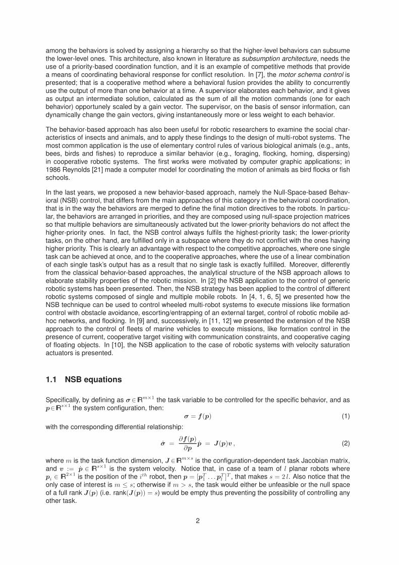
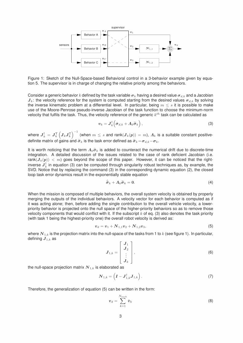
Figure 1: Sketch of the Null-Space-based Behavioral control in a 3-behavior example given by equa-

tion 5. The supervisor is in charge of changing the relative priority among the behaviors.

Consider a generic behavior k defined by the task variable σk having a desired value σd,k and a Jacobian

Jk: the velocity reference for the system is computed starting from the desired values σd,k by solving

the inverse kinematic problem at a differential level. In particular, being m ≤ s it is possible to makeuse of the Moore-Penrose pseudo-inverse Jacobian of the task function to choose the minimum-norm

velocity that fulfils the task. Thus, the velocity reference of the generic kth task can be calculated as

vk = J†k

(σd,k + Λkσk

), (3)

where J†k = JT

k

(JkJT

k

)−1

(when m ≤ s and rank(Jk(p)) = m), Λk is a suitable constant positive-

definite matrix of gains and σk is the task error defined as σk =σd,k−σk.

It is worth noticing that the term Λkσk is added to counteract the numerical drift due to discrete-time

integration. A detailed discussion of the issues related to the case of rank deficient Jacobian (i.e.rank(Jk(p)) < m) goes beyond the scope of this paper. However, it can be noticed that the right-

inverse J†k in equation (3) can be computed through singularity robust techniques as, by example, the

SVD. Notice that by replacing the command (3) in the corresponding dynamic equation (2), the closed

loop task error dynamics result in the exponentially stable equation

˙σk + Λkσk = 0. (4)

When the mission is composed of multiple behaviors, the overall system velocity is obtained by properly

merging the outputs of the individual behaviors. A velocity vector for each behavior is computed as if

it was acting alone; then, before adding the single contribution to the overall vehicle velocity, a lower-priority behavior is projected onto the null space of the higher-priority behaviors so as to remove those

velocity components that would conflict with it. If the subscript k of eq. (3) also denotes the task priority(with task 1 being the highest-priority one) the overall robot velocity is derived as:

vd = v1 + N 1,1v2 + N1,2v3, (5)

where N1,k is the projection matrix into the null-space of the tasks from 1 to k (see figure 1). In particular,

defining J1,k as

J1,k =

J1

J2

...Jk

, (6)

the null-space projection matrix N1,k is elaborated as

N 1,k =(I − J

†1,kJ1,k

). (7)

Therefore, the generalization of equation (5) can be written in the form:

vd =

Ntask∑

k=1

vk (8)

3

sensors

Behavior C

vC v3“

I − J†2J2

”

Behavior B

vB v2 P

“

I − J†1J1

”

Behavior A

vA v1 P

vd

supervisor

Figure 2: Sketch of the Null-Space-based Behavioral control in a 3-behavior example given by equa-

tion 9.

with

vk =

{v1 if k = 1N 1,k−1vk if k > 1.

A detailed convergence and stability analysis of the closed loop task error dynamics is reported in [3]

where the concepts of orthogonality and independency are introduced. In the cited paper, it is also

shown that the solution given by equations (6-8) gives rise to stable and convergent task error dynamicsunder very mild conditions on the task Jacobians Jk and J1,k. Moreover, under stronger assumptions

related to the orthogonality and independency of the task Jacobians involved, also the solution

vk =

{v1 if k = 1(I − J

†1J1

). . .

(I − J

†k−1Jk−1

)vk if k > 1.

(9)

gives rise to convergent and stable closed loop task error dynamics. This solution can be represented

via the block schema in figure 2.

To elaborate the velocity commands to the robots, the NSB control merges behaviors that have been

defined in advance and arranged in priority. However, the design choices concerning how to define

the elementary behaviors to achieve the assigned mission, and how to organize them in priority shouldbe further discussed. These choices derive from practical considerations related to both the mission

objective and the hardware/software characteristics of the robotic system.

For example, if the mission objective is to move the team of robots toward a desired area, we can definea behavior that controls the mean position of the robotic system. This behavior can be analytically

described through a task function that elaborates the centroid position of the team; in a 2-dimensionalcase the task function is expressed by:

σc = fc (p1, . . . , pn) =1

n

n∑

i=1

pi.

where pi =[xi yi

]t is the position of the vehicle i. Thus, assigning a desired value to this task, we can

compute the velocity commands to the robots elaborated on the base of eq. 3, and move the platoon

toward the desired location.

As a further example, we can define a behavior to make the robots avoid collisions with obstacles or

neighboring robots; this behavior may control the robot’s distance from obstacles to keep it above a

desired safety value.

In a general case, the way the behaviors are defined depends on the mission design approach. In a typ-

ical top-down approach, the roboticist has an overall idea of the mission to assign to the robotic system,and he decomposes the overall mission in elementary sub-problems. For each of them, he defines an

elementary behavior and describes it through a mathematical task function. Then, he defines a priority

order depending on practical consideration (e.g., safety behaviors as obstacle avoidance have alwayshigh priority) or on design choice on which behavior, in the case of conflict, needs to be achieved. In a

4

MissionTasks

NSBvNSB

LLCτ

Robotη, ν

η, νη

Figure 3: Control architecture of the NSB with Low-Level Control.

bottom-up design approach, instead, the roboticist may start by defining a set of elementary behaviors

and arranging them in priority. The global behavior of the system thus emerges as a composition of localbehaviors. A bottom-up approach proves useful when the NSB is used to model and simulate dynamical

systems as, for example, traffic control systems, biological systems, and swarms of robots. However, our

focus is on how to define the behaviors when the mission objective are preventively well known. Thus,we mainly use top-down design approaches.

The behavior that controls the centroid positioning of the robots is described through a global task func-tion, that is, a function that needs information about the absolute positions of all the robots of the team.

Such a task function can be easily elaborated in the presence of a centralized system that collects infor-

mation about all the robots. In an indoor environment, a global positioning estimation can be achievedvia a ceiling vision system that sees all the robots. In an outdoor scenario, the robots can use their abso-

lute localization system (as the GPS) and send this information to the central unit via the communication

network. Once all the information has been collected, the central unit elaborates the desired velocity foreach robot on the basis of eq. 3.

Although global behaviors can be useful to achieve missions where we need global control of the teampositioning (as formation control or entrapping/escorting of a target), their usage is not allowed for dis-

tributed robotic systems where each robot has only access to local information. In the latter case, only

decentralized behaviors can be used; that is, behaviors defined for an individual robot, and that onlyuses local information concerning the robot’s neighbors (e.g., the relative positioning or the distance

from its neighbors) or information provided by its local sensors. In this case, the behavior of the team

emerges as a composition of local behaviors, similarly to the case of the bottom-up design approach;however, in this case the roboticist is required to design local behaviors that, individually implemented

on board each robot, make the overall team perform as request for the specific mission.

In this section we want to discuss how the NSB can be used with different robotic systems, e.g., wheeled,

marine or flying robots. It is worth noticing that the NSB performs all the computations considering the

robots as material points with first order dynamics; thus, its output is a linear velocity vector for eachone of the robots. Depending on the robot kinematical and dynamical characteristics, this velocity vector

may or may not be instantaneously achieved by the vehicle. For example, a non-holonomic robot (e.g.,

with unicycle-like or car-like kinematics) cannot instantaneously move in all the directions. In fact, itcan move in the forward direction and rotate, but it cannot move in the lateral direction. Thus, when a

desired velocity vector is assigned to it, the robot can not realize the desired motion if its orientation is

not aligned with the desired velocity vector, but a proper maneuver that modifies its orientation needsto be performed. To this aim, a Low-Level Control (LLC) is designed for the specific kinematic/dynamic

structure of the robot to make it turn and follow the linear velocity vector received by the NSB. As shownin figure 3, the output vector of the NSB is given as a reference value to the LLC that, considering the

kinematical and dynamical characteristics of the robots, is demanded to define the commands to the ac-

tuators (e.g. wheels velocities in the case of grounded robots, thrusters command in the case of marinerobots). This two-level control loop organization allows the usage of the NSB strategy with different kinds

of robotic systems neglecting their kinematical and dynamical characteristics (e.g., omnidirectional/non-

holonomic wheeled robots, or fully-actuated/under-actuated marine robots). These aspects, instead, areconsidered by the LLC that is properly designed for specific robotic system.

Depending on the complexity of the mission, the set of active behaviors may change during the courseof the mission. In this case, a supervisor module is also designed to decide, depending on the mission

stage and using information about the environment, the active behaviors, their priorities and their refer-

ence values. For example, the supervisor can be organized as a finite state machine where, for eachstate, a set of behaviors is defined and their reference values are elaborated. This information is then

5

Robot 1

SupervisorTasks

NSBvNSB

LLCτ

Robotη, ν

η, νηη

η, SupervisorState

Robot 2

SupervisorTasks

NSBvNSB

LLCτ

Robotη, ν

η, νηη

Figure 4: Sketch of the control architecture with two cooperative robots.

given to the NSB module. Moreover, when the robots of a distributed system are commanded to execute

a cooperative mission, they may also need to communicate with their neighbors; in this case, the super-

visor is also in charge of managing the communication. A sketch of the described control architecturefor a two-robot system is reported in figure 4.

2 The software architecture

The proposed architecture is completely decentralized, i.e., each vehicles decides its own motion com-

mands based only on local information gathered by the own sensors or/and by communication with theneighbors. The structure of the robots’ architecture is shown in Figure 5.

Behaviors

Supervisor

ActionsNSB

Actuators Sensors

Real Robot Simulator

Supervisor Level

Action Level

Robot Level

Figure 5: Sketch of the control architecture.

As it can be seen in Figure 5, the control architecture is composed by three layers. Starting from the toplayer, they are the Supervisor Level, the Action Level and, finally, the Robot Level. The first two levels

are abstract levels. In particular, the Action Level defines the set of actions the robot can undertake.

Clearly, the set of actions depends on the mission to be achieved, involving different skills. This meansthat the architecture does not depend on the particular mission, but can be applied to different missions

by properly defining the action set. Once the actions have been defined, each robot chooses the proper

action to perform, according to its internal state and environmental information. To this aim, a Supervisorneeds to be designed. Finally, the Robot Level comprises the computing hardware/software and the

mechanical features of the single robot; the structure of this layer depends on the adopted robotic

6

platform and is primarily concerned with the available sensors and actuators. Further details can be

found in [18].

With regards to the software, it has been developed by means of the Matlab programming language [17]

under Matlab 7.10.0.499 R2010a release and an Object-Oriented Programming (OOP) paradigm. Thedirectory organization into the main source directory (that from now on will be referred as “./“) is the

following:

• @Environment: this directory contains the definition of the class Environment

• @Vehicle: this directory contains the definition of the class Vehicle

• Utility: it contains utility functions used both by the Environment and the Vehicles classes.

The basic idea behind the designed software is that the Environment class encodes all the information

about the environment into where the vehicles are moving, while the Vehicle class encodes all the

information about the vehicle and that each vehicle has its own estimation of this environment. Thisconcept is implemented by designing the Vehicle class in such a way it is a container of the Environment

class.

2.1 The utility functions: in ./Utility

The directory ./Utility contains all the .m functions used by the Environment and the Vehicle classes toallow some functionalities not directly available among the built-in Matlab functions.

2.1.1 The function DiscretizeEnv.m

• DescriptionThis function builds a grid of the environment starting from its boundaries with a given resolution.

This is useful for the domain discretization and the vehicles’ motion as will be clarified in thefollowing. It is not required the environment to be squared or convex.

• Input

1. Vertices (double): matrix [n × 2] containing the vertices of the environment boundaries (sup-posed to be a polygon).

2. Resolution (double): positive scalar value defining the horizontal and vertical distance be-tween to consecutive points in the grid.

• Output

1. X (double): vector [m × 1] containing the x-coordinates of the grid points. The elements

are ordered in such a way that, first, the elements of first row of the grid are stacked into

the vector, then, the elements of the second row and so on. he value of m depends on thepolygon and on the desired resolution.

2. Y (double): vector [m × 1] containing the y-coordinates corresponding to the x-coordinates.The value of m depends on the polygon and on the desired resolution.

• Auxiliary used functions

1. meshgrid.m: this is a built-in Matlab function used to build a first guess of the grid (type “help

meshgrid.m” on the matlab prompt for further information).

2. inpolygon.m: this is a built-in Matlab function used to decide whether a point generated by

meshgrid is in the input polygon or not (type “help inpolygon.m” on the matlab prompt for

further information).

7

2.1.2 The function DistFromPolygon.m

• DescriptionThis function evaluates the distance of a point from a given polygon specified by its vertices.

• Input

1. X (double): vector [n× 1] containing the x-coordinates of the points of which to calculate thedistance from the polygon.

2. Y (double): vector [n× 1] containing the y-coordinates corresponding to the x-coordinates of

the points of which to calculate the distance from the polygon.

3. Vertices (double): matrix [k × 2] containing the vertices of the environment boundaries (sup-posed to be a polygon).

• Output

1. d (double): vector [n × 1] containing the distances of the corresponding input points from the

polygon (defined as the minimal distance from point to any of polygon’s ribs, positive if thepoint is outside the polygon and negative otherwise).

2. x_poly (double): vector [n× 1] containing the x-coordinates of the point in the polygon closest

to X,Y inputs.

3. y_poly (double): vector [n× 1] containing the y-coordinates of the point in the polygon closestto X,Y inputs.


1. inpolygon.m: this is a built-in Matlab function used to decide whether a point generated by

meshgrid is in the input polygon or not (type “help inpolygon.m” on the matlab prompt for

further information).

2.1.3 The function FindDelaunayNeighbors.m

• Description

This function evaluates the indexes of Delaunay neighbors of a given point starting from the delau-

nay triangulation as given by delaunay.m.

• Input

1. DelaunayAdj (int): matrix [n × 3] a such that each row defines a set of triangles such that nodata points in input to the delaunay.m function are contained in any triangle’s circumcircle.

Each row of the matrix defines one such triangle and contains indices into the vectors X and

Y in input to the delaunay.m.

2. NeighborsOf (int): integer scalar index into the vectors X and Y in input to the delaunay.m of

which to calculate its neighbors.

• Output

1. NehigBorsID (int): vector [m × 1] containing the indexes into the vectors X and Y in input to

the delaunay.m of the nehigbors of the point with index NeighborsOf.


1. delaunay.m: this is a built-in Matlab function used to calculate the delaunay triangulation of a

set of points (type “help delaunay.m” on the matlab prompt for further information).

8

2.1.4 The function TransformPoints.m

• DescriptionThis function is able to perform the frame transformation given a list of points and a trasformation

matrix from a frame O1 to a frame O2.

• Input

1. MatrixTransf (double): matrix [3×3] representing the transformation matrix between two planar

frames.

2. ToTransfPoint (double): vector [n× 2] of the points to be transformed such as P = [X Y ] withX and Y of dimension [n × 1].

• Output

1. TrasfPoint (double): vector [n×2] containing the transformed points corresponding to the input

ToTransfPoint such as TrasfPoint=[X Y ] with X and X of dimension [n × 1].


No auxiliary functions have been used.

2.1.5 The function RandomPointsPolyhedron.m

• Description

This function is able to generate random points inside a polygon. It is useful to randomly initializethe vehicles’ positions in the environment.

• Input

1. Vertices (double): matrix [n × 2] containing the vertices of the environment boundaries (sup-

posed to be a polygon)

2. Resolution (double): positive scalar value defining the horizontal and vertical distance be-tween to consecutive points in the grid

3. n (int): positive integer scalar value defining the number of random points to generate.

• Output

1. Points (double): vector [n × 2] containing the randomly generated points such as Points =[X Y ] with X and Y of dimension [n × 1].



2.2 The class Environment: @Environment/Environment.m

The class Environment encodes all the information about the environment the robots are moving in, as,

for example, boundaries, the obstacles’ positions, and so on. Further details are in the following. All the

class’ properties and methods are described in the file Environment.m.

2.2.1 The class Attributes

1. Vertices (double): matrix [n × 2] containing the vertices of the environment boundaries (supposed

to be a polygon).

9

2. ObstaclePos (double): matrix [m×2] containing the points at which the static obstacles are located.

If empty, no obstacle is present.

3. ObstacleRadius (double): vector [m × 1] containing the radius of the circles centered in Obstacle-Pos and containing the obstacles. If empty, no obstacle is present.

4. ImageFile (string): string containing ”path/Image.jpg“, i.e., the image file containing the scenario

in which the vehicles are moving. This property does need to be set in the case the displayfunctionalities of the class are not used.

5. ImageRes_KM_per_Pix (double): positive scalar parameter containing the resolution of the image,or better, the kilometers in the real environment corresponding to each pixel in the image file

ImageFile. This property does need to be set in the case the display functionalities of the classare not used.

6. TrasfMatrix_Image2Coordinate (double): matrix [3 × 3] containing the traformation matrix (with

traslational part in Km) between the reference frame in which the vehicles are moving and defined

by the V ertices property and the Matlab image reference frame (see Matlab documentation). Thisproperty does need to be set in the case the display functionality of the class are not used.

7. Grid (struct): structure containing two fields: vector X (Grid.X) with dimension [k×1] representing

the x-coordinates of the grid discretization domain (defined by the Vertices property); vector Y

(Grid.Y ) with dimension [k × 1] representing the y-coordinates of the grid discretization domain(defined by the Vertices property).

8. VisitedTime (double): vector [k × 1] containing the last time instant each point of the grid Grid has

been visited by some vehicle. Useful in the case of patrolling missions.

2.2.2 The class Methods

The class methods define the functionality implemented by the class useful to access/set the class

attributes.

1. Environment(. . . )

• DescriptionThis is class constructor that initializes the object properties.

• Input

(a) Vertices (double): matrix [n × 2] containing the vertices of the environment boundaries

(supposed to be a polygon).

(b) varargin: this is the standard Matlab variable that allows to call the method with a variable

number of input parameters. The optional input parameters are:

– ResolGrid (varargin{1}) (double): positive scalar value defining the horizontal and

vertical distance between to consecutive points in the grid with which the environmenthas been discretized.

– ImageFile (varargin{2}) (string): the value of the ImageFile property.

– ImageRes_KM_per_Pix (varargin{3}) (double): the value of the ImageRes_KM_per_Pixproperty.

– ObstaclePos (varargin{4}) (double): the value of the ObstaclePos property.

– ObstacleRadius (varargin{5}) (double): the value of the ObstacleRadius property.

– TrasfMatrix_Image2Coordinate (varargin{6}) (double): the value of the

TrasfMatrix_Image2Coordinate property.

• OutputNo outputs are present.

10


(a) DiscretizeEnv.m: this function discretizes the environment and is contained in the ./Utility

directory.

(b) ComputeTrasformationMatrix.m: this is a method of the class described in the following.

2. EvaluatePhi(. . . ):

• Description

This function evaluates the scalar field (whatever is its meaning) used to define the robots’motion strategy in order to satisfy some objective function. An example of function Φ is de-

scribed in Sections 3-5. The expression of this function is encoded in the method itself; futureversions could accept the expression as an additional input parameter.

• Input

(a) CurrentTime (double): the current simulation time in s for time-varying Φ scalar fields.

(b) varargin: this is the standard Matlab variable that allows to call the method with a variable

number of input parameters. The optional input parameters are:

– VerticesPartition (varargin{1}) (double): matrix [m × 2] containing the vertices of thepolygon ( contained in the one defined by the property class Vertices) in which to

evaluate the Φ function. The points in which the function is evaluated are the onesstored in the Grid property and contained in the input polygon.

– Xo (varargin{1}) (double): vector [n×1]. Alternatively to VerticesPartition it is possibleto directly specify the points in which to calculate the Φ function. Xo are the x-

coordinates.

– Y o (varargin{2}) (double): vector [n×1]. Alternatively to VerticesPartition it is possible

to directly specify the points in which to calculate the Φ function. Y o are the y-coordinates.

• Output

(a) Phi (double): vector [n × 1] containing the evaluated scalar field Φ.

(b) varagout: this is the standard Matlab variable used in the case of a variable number of

output parameters requested by the user. Optional outputs can be requested in the case

the user requests the points in which the Φ function has been evaluated (for example, inthe case these points are not given as an input):

– Xo (varagout(1) (double):vector [n × 1] containing the x-coordinates of the points in

which the scalar field has been evaluated.

– Yo (varagout(2) (double):vector [n × 1] containing the y-coordinates of the points in

which the scalar field has been evaluated.


(a) inpolygon.m: this is a built-in Matlab function used to decide whether a point generatedby meshgrid is in the input polygon or not (type “help inpolygon.m” on the matlab prompt

for further information).

(b) meshgrid.m: this is a built-in Matlab function used to build a first guess of the grid (type

“help meshgrid.m” on the matlab prompt for further information).

3. plotPartition(. . . ):

• DescriptionThis is a display utility function that roughly makes a surf of the Φ field in a given polygon.

• Input

(a) CurrentTime (double): the current simulation time in s for time-varying Φ functions.

(b) VerticesPartition (varargin{1}) (double): matrix [m× 2] containing the vertices of the poly-

gon contained in the one defined by the property Vertices in which to evaluate the Φfunction. The points in which the function is evaluated are the ones stored in the Gridproperty and contained in the input polygon.

11

• Output

No outputs are present. A single plot is performed.


(a) inpolygon.m: this is a built-in Matlab function used to decide whether a point generated

by meshgrid is in the input polygon or not (type “help inpolygon.m” on the matlab promptfor further information).

(b) EvaluatePsi: this is a method of the designed class.

4. plotInFigure(. . . ):

• DescriptionThis is a display utility function (eventually to be called at each iteration step) that makes a

representation of the environment together with the vehicles in it, in an image file representing

an harbor or any other facility and stored in the ImageFile property. The function is in chargeto perform any transformation between the real word frame and the image frame thanks the

function TransformPoints.m.

• Input

(a) varargin: this is the standard Matlab variable that allows to call the method with a variablenumber of input parameters. The optional input parameters are:

– PosVehicles (varargin{1}) (double): matrix [k × 2n] containing the vehicles’ positions(not in the image frame) in the environment.

The positions are arranged as [X1 Y 1 X2 Y 2 . . . , Xn Y n] where Xi and Y i are

vectors [k × 1] defining the time history of the i -th vehicle’ positions.

– PosObstacles (varargin{2}) (double): matrix [l × 2no] containing the obstacles’ posi-tions (not in the image frame) in the environment.

The positions are arranged as [X1 Y 1 X2 Y 2 . . . , XnoY no

] where Xi and Y i are

vectors [l × 1] defining the time history of the i -th obstacle’s positions. It is useful fprdynamic obstacles.

• Output

No outputs are present. A single plot is performed.


(a) TransformPoints: an utility function contained in the ./Utility directory.

2.3 The class Vehicle: @Vehicle/Vehicle.m

The class Vehicle encodes all the information about the vehicle as its current position, its past positionsor the current target. Further details are in the following. All the class’ properties and methods are

described in the file Vehicle.m.

2.3.1 The class Attributes

1. ID: positive integer number representing the ID number of the vehicle that allows to distinguisheach vehicle from the others.

2. PositionHistory (double): vector [n × 2] whose i -th row represents the vehicle’s position at time ti.The vector dynamically grows with time.

3. CurrentTime (double): current simulation time in s.

4. CurrentTarget (double): current target to reach.

5. SampleTime (double): simulation sample time in s used to perform the numerical integration of the

velocity commands.

12

6. MaxVel (double): maximum linear velocity of the vehicle in Km/h.

7. EnvEstimate (object): this is an object of the class Environment described in Section 2.2 and that

stores an estimates of the environment has built by the particular vehicle object instance.

2.3.2 The class Methods

The class methods define the functionality implemented by the class useful to access/set the class

attributes.

1. Vehicle(. . . )

• DescriptionThis is class constructor that initializes the object properties.

• Input

(a) ID (int): the vehicle ID property.

(b) InitialPosition (double): the vehicle’s initial position to be stored in the CurrentPosition

property.

(c) SampleTime (double): the simulation sample time to be stored in the SampleTime prop-

erty.

(d) MaxVel (double): the maximum linear velocity allowed by the vehicle to be stored in the

MaxVel property.

(e) Vertices (double): the vertices of the polygon describing the environment to be passed at

the constructor of the Environment class (see Section 2.2 ).

(f) ResolGrid (double): the grid resolution with which to discretize the environment to bepassed at the constructor of the Environment class (see Section 2.2 ).

• Output

No outputs are present.

• Auxiliary used functionsNo auxiliary functions have been used.

2. MoveToGoal(. . . )

• Description

This method allows to reach the current target thanks to the Reach Target behavior. Refer to

Section 3.3 for details. This function should be called at each iteration step.

• Input

(a) CurrentTime (double): the current simulation time in s.

• Output

No output is present. This function updates the object’s CurrentPosition and the Position-History properties.


No auxiliary functions have been used

3. AvoidObstacle(. . . )

• Description

This method allows to reach the current target while avoiding obstacles stored in the properfields of EnvEstimate property. Refer to Section 3.4 for details. This function should be called

at each iteration step.

• Input

(a) CurrentTime (double): the current simulation time in s.

13

• Output

No output is present. This function updates the object’s CurrentPosition and the Position-History properties.



4. ChooseNextTarget(. . . )

• DescriptionThis function is the Supervisor of the vehicle. It implement any strategy suitable to accomplish

the given mission. It could be, for example, a State Automata, a Fuzzy Logic Supervisor, or

any implement any other more complicated policy. This function should be called at eachiteration step.

• Input

(a) VoronoiPartition (double): matrix [n× 2] defining the voronoi partition in which the vehicle

is.

• Output

(a) NextTarget (double): vector [n × 1] defining the next target. The CurrentTarget property

is updated. It could be equal to the previous target according to the Supervisor’s policy.


(a) DistFromPolygon.m: contained in the ./Utility directory and that evaluates the distance of

a point from a given polygon.

5. ReceiveSamplesFrom(. . . )

• Description

This function allows to gather information from the Delaunay neighbors in order to get a moreprecision estimation of the vector field Φ. This functionality is useful in the case of function

field built on line and to implement decentralized strategies.

• Input

(a) SenderID (int): positive integer scalar value defining the ID property of the sender vehicle.

(b) Data (double): matrix [n × x] defining the vector of data exchanged (stored as rows).

The x dimension depends on the data exchanged and is, for example, 2 in the case ofexchanged positions.

(c) AtTimes (double): vector [n × 1] such as the i -th element represents the time instant at

which the corresponding Data is referred to. This is useful in the case of a time varying

fields Φ.

• OutputNo outputs are present. Simply, the internal representation of the environment is updated.



6. SendSamplesTo(. . . )

• DescriptionThis function sends answers to a data request from another vehicle in order to allow a more

precision estimation of the vector field Φ. This functionality is useful in the case of function

field built on line and to implement decentralized strategies.

• Input

(a) ReceiverID (int): positive integer scalar value defining the ID property of the receiver

vehicle.

(b) VoronoiPartOfReceiver (double): matrix [n × 2] defining the voronoi partition of the re-

ceiver vehicle useful to the sender to establish the information effectively needed by thereceiver in order to build a precise information of the field Φ inside its partition.

14

(c) CurrentTime (double): the current simulation time useful in the case of time varying filed

Φ.

• Output

(a) UpdatePoints (double): matrix [n × x] defining the vector of data exchanged (stored as

row). The x dimension depends on the data exchanged and is, for example, 2 in the caseof exchanged positions.

(b) AtTimes (double): vector [n × 1] such as the i -th element represents the time instant atwhich the corresponding Data is referred to. This is useful in the case of a time varying

field.


(a) DistFromPolygon.m: contained in the ./Utility directory and that evaluates the distance ofa point from a given polygon.

7. getPath(. . . )

• Description

This function has as output the position history of the vehicle.

• InputNo input parameters are present.

• Output

(a) Path (double): vector [n × 2] of the time history of the vehicle’s positions. The sample

time is specified by the object’s SampleTime property.

• Auxiliary used functionsNo auxiliary functions have been used.

8. getCurrentPosition(. . . )

• Description

This function has as output the current position of the vehicle as stored in the CurrentPosition

property.

• Input

No input parameters are present.

• Output

(a) CurrentPosition (double): vector [1 × 2] of the current position of the vehicle.



9. getCurrentTarget(. . . )

• Description

This function has as output the current target to be reached by the vehicle as stored in theCurrenttarget property.

• Input


• Output

(a) CurrentTarget (double): vector [1 × 2] of the current target of the vehicle.



10. getPath(. . . )

• Description

This function has as output the position history of the vehicle as stored in the PositionHistoryproperty.

15

• Input


• Output

(a) Path (double): vector [n × 2] of the time history of the vehicle’s positions. The sample

time is specified by the object’s SampleTime properly.

• Auxiliary used functionsNo auxiliary functions have been used

11. PlotEnv(. . . )

• Description

This function simply calls the plotInFigure() method of the EnvEstimate property. The impor-

tant fact is that the environment is an estimate of the real one as built by the vehicle.

2.4 Main Loop

The above functions and classes are used within a main simulation loop. The main file (MAIN_FILE.mcontained in the source directory) is in charge of instantiating the objects with a proper initialization by

means of the class constructor. The Algorithm 1 gives a sketch of the main file.

Algorithm 1 Algorithm describing the main simulation script.

Initialization Sectiondefine n: number of vehicles

define matrix Vertices: environment boundariescreate the n vehicle objects by calling the class constructor

End Initialization Section

loopfor i = 1 to n do

1) build V or(xr,i) based on local information, where xr,i is the i -th vehicle’s position.

2) request updating data to local neighbors in the case of cooperative on-line estimation of the

density function Φ ( ReceiveSamplesFrom(. . . ) )3) update of the field Φ estimation

4) choose the next point to reach ( ChooseTheNexttarget(. . . ) )

5) apply the MoveToGoal(. . . ) or ObstacleAvoidance(. . . ) behavior.6) perform some display functionality

7) increase the time variableend for

end loop

3 One case study: deployment

Among the various control problems involving multiple robots one important is given by the deployment.

Roughly speaking, the deployment problem consists in the optimal placement of the robots within a givenenvironment. The cooperarive deployment can be seen as a sampling problem and it is a topic gaining

interest from the community, see, e.g., [23]. One significant contribution is given by [14] and [19] wherea proper scalar index function is proposed and optimized by a gradient-based, distributed, discrete-time

approach. The above cited papers exploit the mathematical properties of the Voronoi partitions, deeply

discussed by [20] with several interesting applications in mathematics and engineering as developedby [16]. Voronoi partition of a set is characterized by an appealing list of properties: the partitions

16

are not overlapping, their union gives back the original set and, most important, their computation is

distributed; it is thus clear that this is the key to distribute among robots a global index.

The i th robot position is denoted as xi ∈ IRl, l = 2, 3. The vector x ∈ IRln collects the positions of all

the n robots.

In this paper, the dynamics of the robots will be considered as a single integrator, i.e., xi = ui with ui ∈IRl with a corresponding collective dynamics:

x = u (10)

with u ∈ IRln.

3.1 Voronoi

The Voronoi partitions (or diagrams) are a subdivisions of a set S characterized by a metric with re-spect to a finite number of points belonging to the set. Given a set {x1, x2, . . . , xn} with xi ∈ IRl, the

corresponding n Voronoi cells, V or(xi), are given by:

V or(xi) = {s ∈ S | ‖s − xi‖ ≤ ‖s − xj‖ ∀j} .

Figure 6 reports the Voronoi decomposition of a bidimensional with respect to randomly generatedpoints.

Figure 6: Voronoi partitions of a 2-dimensional (l = 2) set.

As stated into the Introduction, the computation of the Voronoi cells is structurally decentralized: each

point xi can compute the corresponding cell V or(xi) by simply knowing its position and the neighbors’positions. The term neighbor indicates a point xj that is close to xi given a certain metric (for example

the euclidean distance). Details on the Voronoi-based theory can be found in [20] or [16].

3.2 The deployment problem

The deployment problem consists in the optimal placement of the robots within a given environment

according to some criteria. Given a convex set S, the basic idea is to build a proper function to be mini-mized (maximized) that properly takes into account two different requirements. An example of criterion

17

can be the necessity to deploy the robots in some places according to a scalar density function Φ ∈ IR

that may represent, for example, the probability that some interesting events take place in a certain point.For example, in the case of a marine scenario, the function Φ may represent some disaster place, oil

spill or important facilities’ locations. However, it is necessary to distribute the robots over the region,avoiding that they all locate in the most interesting point, according to a positive non-decreasing scalar

performance function f ∈ IR. This can be formulated from a mathematical point of view with a scalar

function σ(x) ∈ IR to be minimized:

σ(x) =

∫

S

mini

f(‖s − xi‖)Φ(s)ds.

It is known from [16] that this integral index may be rewritten according to local contributions by resortingto the Voronoi partitions. This idea has been later considered also by [14]:

σ(x) =1

2

n∑

i=1

∫

V or(xi)

f(‖s − xi‖)Φ(s)ds (11)

where s ∈ IRl is the generic point of the set S, the set V or(xi) is the Voronoi partition associated to

the i th robot and Φ(s) ∈ IR is a proper density function. One possible choice is f = ‖s − xi‖2

=

(s − xi)T

(s − xi) leading to the problem defined as distortion problem by [14].

The associated Jacobian J(x) =∂σ

∂x∈ IR1×ln is structurally decoupled and exhibits the structure:

J =[· · ·

∫V or(xi)

Φ(s) (s − xi)T

ds · · ·]

(12)

where the generic term reported is an (1 × l) matrix. Notice that the partial derivative of eq. (11) is nottrivial, details can be found in [14].

It is worth noticing that, in order to compute the Jacobian it is necessary to know the absolute robot

position, the density function and the neighbors positions. It is also interesting to observe that theJacobian can be rewritten as

J =[· · · m(xi) (c(xi) − xi)

T· · ·

](13)

where

m(xi) =

∫

V or(xi)

Φ(s)ds

c(xi) =

∫V or(xi)

sΦ(s)ds∫

V or(xi)Φ(s)ds

are the scalar mass and the l-dimensional centroid of the i- th Voronoi partition, respectively. A straight-forward interpretation is that the stationary points of this function are the centroids of the Voronoi par-

titions. Then, the problem becomes to find the Voronoi partitions such that the position of vehicles

coincides with the respective partition’s centroids. Such a configuration is called centroidal Voronoi con-figuration and is, in general, not unique. A general way to reach such a configuration is the Lloyd’s

method well described in [16], where, in a few words, the robots move towards the centroids of theirpartition while updating the overall Voronoi tessellation.

A central aspect in this approach is that the function Φ(s) is required to be fully known over the integration

domain. This can seem an unrealistic hypothesis in many applications, but this aspect will not beentaken into account in this paper. However it is worth saying that it is a topic of ongoing research and,

for example, in [22] a way to iteratively estimate the function Φ(s) is adopted. In the case of surface

vehicles that is the case addressed in this paper, it might be supposed that there is a main vessel ableto communicate to the other vehicles the estimation of the density function.

18

3.3 The Reach centroid task

According to the Section 3.2, the deployment task consists in finding the centroidal Voronoi configura-tions. Being the task completely decoupled, based on the method described in [16], each robot has to

reach the centroid of its Voronoi partition, this means that the velocity of the i-th vehicle can be calculated

as:

σrc,i = ‖xi − c(xi)‖, σrc,d = 0,

Jrc,i = rTrc,i, J

†rc,i = rrc,i,

urc,i = λrcrrc,i (−σrc,i) ,

(14)

with rrc,i = [xi − c(xi)] /‖xi − c(xi)‖, λrc positive scalar gain, and urc,i is the corresponding velocity of

i-th robot.

3.4 Obstacle avoidance

An important task when dealing with AUV vehicles in unknown environments is the obstacle avoidance

task. Herein, obstacles are represented by other vehicles or other static objects in the environment. Thedistance of the single robot from the obstacle can be controlled by the function σ(xi) ∈ IR

σ(xi) =1

2(xi − c)T(xi − c),

where c ∈ IRl represents the obstacle’s coordinates. In this case the sole i th robot is concerned by this

function and the corresponding Jacobian J ∈ IR1×ln is reflecting this property

J =[0

Tl . . . (xi − c)T . . . 0

Tl

].

Also in this case the task is completely decoupled, then

σoa,i = ‖xi − c‖, σoa,d = ds,

Joa,i = rToa,i, J

†oa,i = roa,i,

Noa,i = I − roa,irToa,i

voa,i = λoaroa,i (ds − σoa,i) ,

(15)

where λoa is positive scalar gain, ds is the safety distance taking into account the dimension of the

obstacle and uoa,i is the corresponding velocity of i th robot. This tasks avoid the i th vehicle to enter the

circle centered in c and radius ds.

4 Proposed solution

As stated in Section 3.2, the calculation of the Voronoi tessellation is completely distributed, this means

that the calculation of eq. (11) only requires each robot takes into account the other robots that are in

neighborhood. In addition, the obstacle avoidance too is a local objective function.

The robots are thus commanded under eq. (14) when no obstacles lies within its field of view, thus

minimizing also the velocity norm. When an obstacle is in front of the vehicles the velocity is generated

according to eq. (8) where the higher priority task is the obstacle avoidance, and the reach centroidvelocity urc,i is projected into the null space of the obstacle avoidance task by means of the null projector

matrix Noa,i. The switch between the two states, one with a single task function (reach centroid) and theother with two tasks (obstacle avoidance and reach centroid), is achieved by a simple supervisor with

inputs the exteroceptive sensors. Notice that, as evidenced by [2], it is useless to add additional tasks

when the degrees of freedom are already saturated.

19

5 Simulations

Let us consider the 2-dimensional (l = 2) scenario in Figure 7, representing a portion of a gulf situatedin south coast of Italy.

Obstacles

1

2

3

Figure 7: A portion of a gulf situated in south coast of Italy as scenario for the deployment mission. Thedashed circles represent the border of the safety area around the obstacle

The dashed circles represent the border of the safety area around the three present obstacles. The

following values of positions c of the obstacles and of the safety distance ds in equation (15) are consid-ered

Obstacle # Position ds

1 c1 =[6.5 9.8

]TKm 2.20

2 c2 =[9.9 11.0

]TKm 0.9

3 c3 =[16.8 2.5

]TKm 1.55

We suppose the robots are able to navigate at a maximum speed of 4 Km/h, in addition the following

values for the control gains in eq. (14) and eq. (15) are considered:

task gain

λrc 4

λoa 4

The graphical animations of the following case studies can be found at the address:http://webuser.uni as.it/lai/roboti a/video.html5.1 First case study

As a demonstration, we consider the simple case of one vehicle moving in the environment shown in

Figure 7. In addition, we suppose that the function Φ is:

Φ(x, y) = exp(−k(x − bx)2 − k(y − by)2)

where k = 2 and b =[bx by

]T=

[3.9 13

]TKm is the center of a bell-like-shaped function.

In Figure 8, the vehicle’s path for the first case is shown. A contour plot of the function Φ is also depicted,with color from red to blue, corresponding to higher and lower value of the density function, respectively.

20

Start

C1

R1

Figure 8: First case study. The Φ function and the robot path (yellow). C1: centroid of the area (white

point).

As it can be seen, the vehicle reach the center of the function (also the centroid of the area) while

surrounding the obstacle #2. In fact, in Figure 9 (on the top) the time history of the normalized objective

function (11) is represented: the objective function is decreasing along the vehicle trajectory with achange of slope during the obstacle avoidance phase (the primary task); while in the bottom the time

history of the distance from the obstacle is shown.

10

2

4

6

8

0

0

0.2

0.4

0.6

0.8

1

0.5

0.5

1.5

1.5

2.5

2.5

3.5

3.5

4.5

4.5

[Km

][]

Obstacle

time [h]

Objective Function

Distance from the obstacle

Figure 9: First case study. In the top: the time history of the normalized objective function. In the bottom:

the time history of the distance from the obstacle #2 (the dashed line is the safety distance ds for thisobstacle).

5.2 Second case study

As a further example, let us consider the case of four vehicles moving in the same environment. The

density function Φ is defined as:

Φ(x, y) =

4∑

i=1

exp(−k(x − bx,i)

2 − k(y − by,i)2)

where k = 2.5 and each bi =[bx,i by,i

]T∈ IR2 is the center of a bell-like-shaped function ( b1 =

[3 10

]TKm, b2 =

[8.6 11.6

]TKm, b3 =

[13.9 2

]TKm, b4 =

[6 6

]TKm ) . As shown in Figure 10,

21

in this case too, the vehicles reach the centroids (while avoiding obstacles) of their Voronoi partition

(centroidal configuration) in a completely decentralized fashion.

C1

R1

C2

R2

C3 R3

C4

R4

Figure 10: Second case study. Four Vehicles. The Φ function and the robots’ paths (yellow). Cx: centroid(white points) of the Voronoi partition of robot #x. Rx: robot #x.

In Figure 11, the time history of the objective function 11 and of the distance between the robot #1 andthe obstacle are depicted on the top and in the bottom, respectively. In this case, because of the shape

10

12

2

2

2

3

3

4

4

4

5

5

6

8

0

0

0.2

0.4

0.6

0.8

1

1

10.5 1.5 2.5 3.5 4.5

[Km

][]

time [h]

Objective Function

Distances from the obstacles

R1 O1

R2 O2

R3 O3

Figure 11: Second case study. In the top: the time history of the normalized objective function. In thebottom: the time history of the distances of the robot #1 form the obstacle #1, of the robot #2 from the

obstacle #2, of the robot #3 from the obstacle #3 (the dashed lines are the safety distances).

of the density function and the number of robots, the centroids’ positions are also the centers of the

density function. However, in general this is not true. For example, in Figure 12 the robot’s paths areshown in the case of the same shape of the Φ function but with five vehicles. The final configuration is a

Voronoi centroidal configuration but it is not symmetric.

5.3 Third case study

Another interesting application of the approach described in sect. 3.2 is the distributed formation control.

The intuition in [15] is that the shape of the density function Φ can be used to keep the vehicles in the

22

C1

R1

C2

R2

C3

R3

C4R4

C5

R5

Figure 12: Second case study. Five vehicles. The Φ function and the robots’ paths (yellow). Cx: centroid

of the Voronoi partition (white points) of robot #x. Rx: robot #x.

desired formation. Thus, by properly defining the density function Φ, it is possible to roughly assign thedesired positions of the vehicles. Let us consider, for example, the following expression of Φ:

Φ = exp(−k1

(k2(x − bx)2 + k3(y − by)2 − r2

)),

that allows to draw an ellipse of center b =[bx by

]T∈ IR2 with dimension depending on the positive

scalar gains ki and r. A further step can be to assign a time law to the center of the ellipse, i.e., b = b(t),in order to move the formation on the surface. Let us consider five vehicles and the following values

of the gains for the density function: k1 = 2, k2 = 2, k3 = 3 and r = 2; in addition, we suppose thatthe center b of the ellipse slowly moves in the environment in order to satisfy the principle of timescale

separation (i.e., the function Φ varies slowly compared to the dynamics of the robots and the controller).

Moreover, the path is chosen in order to cross the obstacle #1 in order to test the obstacle avoidancetask also in this conditions.

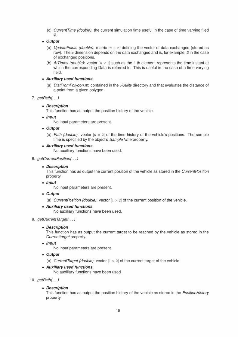
In Figure 13, the robots’ paths are depicted (yellow) together with the path of the Φ function’s center (red).

The robots moves from their initial configuration to the desired formation and keep the formation whilemoving toward the goal. During the motion, the obstacle causes the robots to break the formation as

the obstacle avoidance is always the highest priority task. Once the Φ function has completely crossedthe obstacle, the robot are again able to assume the desired formation. The snapshots of these different

phases are shown in Figure 14.

R1

R2R3

R4

R5

Figure 13: Third case study. The Φ function, its path (red line) and the robots’ paths (yellow)). Rx: robot

#x.

In Figure 15, the time history of the distance between the robos and the obstacle are depicted, also in

this case the collisions are prevented thanks to the priority strategy.

23

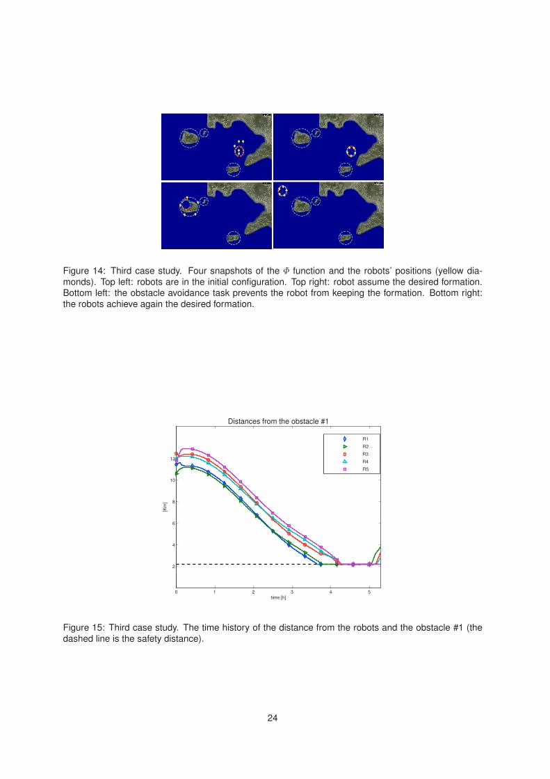
Figure 14: Third case study. Four snapshots of the Φ function and the robots’ positions (yellow dia-

monds). Top left: robots are in the initial configuration. Top right: robot assume the desired formation.Bottom left: the obstacle avoidance task prevents the robot from keeping the formation. Bottom right:

the robots achieve again the desired formation.

0 1

2

2 3

4

4 5

6

8

10

12

time [h]

[Km

]

R1

R2

R3

R4

R5

Distances from the obstacle #1

Figure 15: Third case study. The time history of the distance from the robots and the obstacle #1 (the

dashed line is the safety distance).

24

References

[1] G. Antonelli, F. Arrichiello, and S. Chiaverini. The entrapment/escorting mission: An experimen-tal study using a multirobot system. IEEE Robotics and Automation Magazine (RAM). Special Is-

sues on Design, Control, and Applications of Real-World Multi-Robot Systems, 15(1):22–29, March

2008.

[2] G. Antonelli, F. Arrichiello, and S. Chiaverini. The Null-Space-based Behavioral control for au-tonomous robotic systems. Journal of Intelligent Service Robotics, 1(1):27–39, January 2008.

[3] G. Antonelli, F. Arrichiello, and S. Chiaverini. Stability analysis for the null-space-based behavioral

control for multi-robot systems. In 47th IEEE Conference on Decision and Control and 8th European

Control Conference, Cancun, MEX, December 2008.

[4] G. Antonelli, F. Arrichiello, and S. Chiaverini. Experiments of Formation Control With MultirobotSystems Using the Null-Space-Based Behavioral Control. IEEE Transactions on Control Systems

Technology, 17(5):1173–1182, September 2009.

[5] G. Antonelli, F. Arrichiello, and S. Chiaverini. Flocking for multi-robot systems via the null-space-

based behavioral control. Swarm Intelligence, 4(1):37–56, March 2010.

[6] G. Antonelli, F. Arrichiello, S. Chiaverini, and R. Setola. Coordinated control of mobile antennasfor ad-hoc networks. International Journal of Modelling Identification and Control Special/Inaugural

issue on Intelligent Robot Systems, 1(1):63–71, 2006.

[7] R.C. Arkin. Motor schema based mobile robot navigation. The International Journal of Robotics

Research, 8(4):92–112, 1989.

[8] R.C. Arkin. Behavior-Based Robotics. The MIT Press, Cambridge, MA, 1998.

[9] F. Arrichiello, S. Chiaverini, and T.I. Fossen. Formation control of marine surface vessels usingthe Null-Space-based Behavioral control. In Group Coordination and Cooperative Control, K.Y.

Pettersen, T. Gravdahl, and H. Nijmeijer (Eds.), Springer-Verlag’s Lecture Notes in Control and

Information Systems series, pages 1–19. May 2006.

[10] F. Arrichiello, S. Chiaverini, G. Indiveri, and P. Pedone. The Null-Space based Behavioral controlfor mobile robots with velocity actuator saturations. International Journal of Robotics Research,

29(10):1317–1337, Sept. 2010.

[11] F. Arrichiello, J. Das, H. Heidarsson, A. Pereira, S. Chiaverini, and G.S. Sukhatme. Multi-robot

collaboration with range-limited communication: Experiments with two underactuated asvs. In Pro-ceedings 2009 International Conference on Field and Service Robots, Cambridge, Massachusetts,

USA, July 2009.

[12] F. Arrichiello, H. Heidarsson, S. Chiaverini, and G.S. Sukhatme. Cooperative caging using au-tonomous aquatic surface vehicles. In 2010 IEEE International Conference on Robotics and Au-

tomation, pages 4763–4769, Anchorage, USA, May 2010.

[13] R.A. Brooks. A robust layered control system for a mobile robot. IEEE Journal of Robotics and

Automation, 2(1):14–23, 1986.

[14] F. Bullo, J. Cortés, and S. Martinez. Distributed Control of Robotic Networks. Princeton UniversityPress, 2008.

[15] J. Cortés, S. Martínez, T. Karatas, and F. Bullo. Coverage control for mobile sensing networks.

IEEE Transactions on Robotics an Automation, 20(2):243–255, 2004.

[16] Q. Du, V. Faber, and M. Gunzburger. Centroidal Voronoi tessellations: applications and algorithms.

SIAM review, 41(4):637–676, 1999.

[17] http://www.mathworks.com.

25

[18] A. Marino, L. Parker, G. Antonelli, and F. Caccavale. Behavioral control for multi-robot perimeter

patrol: A finite state automata approach. In Proceedings 2009 IEEE International Conference onRobotics and Automation, pages 831–836, Kobe, J, May 2009.

[19] S. Martinez, J. Cortés, and F. Bullo. Motion coordination with distributed information. IEEE Control

Systems Magazine, 27(4):75–88, August 2007.

[20] A. Okabe, B. Boots, and K. Sugihara. Spatial tessellations: concepts and applications of Voronoidiagrams. John Wiley & Sons, 1992.

[21] C. Reynolds. Flocks, herd and schools: A distributed behavioral model. Computer Graphics,21(4):25–34, 1987.

[22] M. Schwager, D. Rus, and J. J. Slotine. Unifying geometric, probabilistic, and potential field ap-

proaches to multi-robot deployment. International Journal of Robotics Research, 30(3), 2011.

[23] R. Smith, J. Das, H. Heidarsson, A. Pereira, F. Arrichiello, I. Cetinic, L. Darjany, M. Garneau,

M. Howard, C. Oberg, M. Ragan, E. Seubert, E. Smith, B. Stauffer, A. Schnetzerand G. Toro-Farmer, D. Caron, B. Jones, and G. Sukhatme. The USC center for integrated networked aquatic

platforms (CINAPS): Observing and monitoring the southern California bight. accepted for publica-tion IEEE Robotics and Automation Magazine, Special Issue on Marine Robotic Systems, 17(1):20–

30, 2010.

26

deliverable d 5 - jacobs university

Documents