deliverable d 1.3 characterization of the railway

ii

“output” — 2020/1/2 — 20:41 — page 1 — #1 ii

ii

ii

Deliverable D 1.3Characterization of the railway environment:

channel models & general characteristicsProject acronym: EMULRADIO4RAILStarting date: 01/12/2018Duration (in months): 18Call (part) identifier: H2020-S2R-OC-IP2-2018-03Grant agreement no: 826152Due date of deliverable: Month 12Actual submission date: 01/12/2019Responsible/Author: Juan Moreno - MdMDissemination level: PUStatus: Draft

Reviewed: (yes/no)

GA 826152 | 53

Ref. Ares(2020)7942419 - 02/01/2020

ii

“output” — 2020/1/2 — 20:41 — page 2 — #2 ii

ii

ii

Document historyRevision Date Description01 01/12/2019 First issue

Report contributors

NameBenificiaryShort Name

Details of contribution

Juan Moreno MdMContribution on the railway channel choices andglobal review

Romain Behaegel IfsttarContributions on general state of art for channelmodels and railway channel models, help on layouton overleaf

Marion Berbineau IfsttarContributions on general state of art for channelmodels and railway channel models and generalreview

Yann Cocheril Ifsttar Help on Layout on overleafLaurent Clavier Univ. Lille General final review

GA 826152 | 53

ii

“output” — 2020/1/2 — 20:41 — page 3 — #3 ii

ii

ii

Contents

1 Executive Summary 7

2 Abbreviations and acronyms 8

3 Background 9

4 Objectives 10

5 Context 115.1 Railway scenarios (input from T1.1) . . . . . . . . . . . . . . . . . . . . . . . . . . . . 115.2 Perturbations to be introduced (input from T1.2) . . . . . . . . . . . . . . . . . . . . . . 11

6 Mobile radio propagation generalities and modelling 126.1 Introduction . . . . . . . . . . . . . . . . . . . . . . . . . . . . . . . . . . . . . . . . . . 126.2 Main characteristics of the mobile radio channel . . . . . . . . . . . . . . . . . . . . . 12

6.2.1 Multipath . . . . . . . . . . . . . . . . . . . . . . . . . . . . . . . . . . . . . . . 126.2.2 Longitudinal attenuation . . . . . . . . . . . . . . . . . . . . . . . . . . . . . . . 126.2.3 Delay spread . . . . . . . . . . . . . . . . . . . . . . . . . . . . . . . . . . . . . 136.2.4 Doppler effect . . . . . . . . . . . . . . . . . . . . . . . . . . . . . . . . . . . . . 15

7 Mathematical representation of wireless channels 177.1 Representation of the MIMO channel . . . . . . . . . . . . . . . . . . . . . . . . . . . . 187.2 Wide Sense Stationary Channel (WSSUS) [[1] . . . . . . . . . . . . . . . . . . . . . . 207.3 Conclusion . . . . . . . . . . . . . . . . . . . . . . . . . . . . . . . . . . . . . . . . . . 21

8 Mobile Radio channel models 228.1 Introduction . . . . . . . . . . . . . . . . . . . . . . . . . . . . . . . . . . . . . . . . . . 228.2 Non-Geometric Stochastic Channel Model . . . . . . . . . . . . . . . . . . . . . . . . . 22

8.2.1 Introduction . . . . . . . . . . . . . . . . . . . . . . . . . . . . . . . . . . . . . . 228.2.2 Tapped Delay Line channel model . . . . . . . . . . . . . . . . . . . . . . . . . 228.2.3 ITU models . . . . . . . . . . . . . . . . . . . . . . . . . . . . . . . . . . . . . . 238.2.4 Saleh-Valenzuela channel model . . . . . . . . . . . . . . . . . . . . . . . . . . 24

9 Radio channel models based on measurements and simulations in typical railway envi-ronments 259.1 Introduction . . . . . . . . . . . . . . . . . . . . . . . . . . . . . . . . . . . . . . . . . . 259.2 Channel models obtained with measurements and simulations along high speed lines 26

9.2.1 Introduction . . . . . . . . . . . . . . . . . . . . . . . . . . . . . . . . . . . . . . 269.2.2 Train to Ground Tapped Delay line channel model for high speed line scenarios 26

9.3 Train to Ground Cluster Delay line channel model for high speed line scenario . . . . . 349.3.1 Conclusion . . . . . . . . . . . . . . . . . . . . . . . . . . . . . . . . . . . . . . 35

9.4 Channel models obtained with measurements and simulations in tunnels . . . . . . . 369.4.1 Introduction . . . . . . . . . . . . . . . . . . . . . . . . . . . . . . . . . . . . . . 369.4.2 Free propagation in tunnel . . . . . . . . . . . . . . . . . . . . . . . . . . . . . . 369.4.3 Train to Ground channel model for tunnel scenario . . . . . . . . . . . . . . . . 389.4.4 Conclusion . . . . . . . . . . . . . . . . . . . . . . . . . . . . . . . . . . . . . . 39

9.5 General conclusion regarding state of the art related to Channel models for Railwayenvironments . . . . . . . . . . . . . . . . . . . . . . . . . . . . . . . . . . . . . . . . . 40

GA 826152 | 53

ii

“output” — 2020/1/2 — 20:41 — page 4 — #4 ii

ii

ii

10 Applicability analysis of the channel models for the emulation platform 4110.1 Introduction . . . . . . . . . . . . . . . . . . . . . . . . . . . . . . . . . . . . . . . . . . 4110.2 Methodology . . . . . . . . . . . . . . . . . . . . . . . . . . . . . . . . . . . . . . . . . 4110.3 Summary of the channel models most suitable for emulation . . . . . . . . . . . . . . 42

10.3.1 Hilly Terrain . . . . . . . . . . . . . . . . . . . . . . . . . . . . . . . . . . . . . . 4210.3.2 Rural scenario . . . . . . . . . . . . . . . . . . . . . . . . . . . . . . . . . . . . 4210.3.3 Viaduct . . . . . . . . . . . . . . . . . . . . . . . . . . . . . . . . . . . . . . . . 4210.3.4 Cutting . . . . . . . . . . . . . . . . . . . . . . . . . . . . . . . . . . . . . . . . 4310.3.5 Tunnel scenario . . . . . . . . . . . . . . . . . . . . . . . . . . . . . . . . . . . 43

11 Conclusions 44

GA 826152 | 53

ii

“output” — 2020/1/2 — 20:41 — page 5 — #5 ii

ii

ii

List of Figures1 Illustration of multipath phenomenon . . . . . . . . . . . . . . . . . . . . . . . . . . . . 132 Illustration of slow and fast fading . . . . . . . . . . . . . . . . . . . . . . . . . . . . . . 133 Illustration of Power delay profile measured . . . . . . . . . . . . . . . . . . . . . . . . 144 Representation of the Classic Doppler spectrum [2] . . . . . . . . . . . . . . . . . . . . 155 Representation of the Flat Doppler spectrum . . . . . . . . . . . . . . . . . . . . . . . 166 Representation of the Gaussian Doppler spectrum . . . . . . . . . . . . . . . . . . . . 167 Representation of the Rice Doppler spectrum . . . . . . . . . . . . . . . . . . . . . . . 178 Time-varying impulse response representation . . . . . . . . . . . . . . . . . . . . . . 179 Bello functions . . . . . . . . . . . . . . . . . . . . . . . . . . . . . . . . . . . . . . . . 1810 Representation of azimuth and elevation angles . . . . . . . . . . . . . . . . . . . . . . 2011 TDL representation of four taps . . . . . . . . . . . . . . . . . . . . . . . . . . . . . . . 2312 Saleh-Valenzuela representation following exponential decrease [3] . . . . . . . . . . 2513 Classification of High Speed Train environments [4] . . . . . . . . . . . . . . . . . . . . 2714 Description of viaduct scenario from [5] . . . . . . . . . . . . . . . . . . . . . . . . . . 2815 A - Relative positions over the distance. The blue dashed line denotes Dmin, the blue

point represents IP of Dmin and the rail. DAA, DCEA, DCA and DTA are the distancesfrom IP to the corresponding area bound, respectively. B - Schematic illustration ofDCEA . [5] . . . . . . . . . . . . . . . . . . . . . . . . . . . . . . . . . . . . . . . . . . . 29

16 Description of viaduct scenario from [6] . . . . . . . . . . . . . . . . . . . . . . . . . . 2917 Illustration of U-shape cutting scenario corresponding to the TDL model given in table 9 3118 D2a scenario [7] . . . . . . . . . . . . . . . . . . . . . . . . . . . . . . . . . . . . . . . 3419 Evolution of the electric field along tunnel for different frequencies . . . . . . . . . . . 3720 Representation of the scenario simulated [8] . . . . . . . . . . . . . . . . . . . . . . . 3921 Rural environment for HSL in China [9] . . . . . . . . . . . . . . . . . . . . . . . . . . . 43

GA 826152 | 53

ii

“output” — 2020/1/2 — 20:41 — page 6 — #6 ii

ii

ii

List of Tables1 Probability of occurrence P in % for low delay spread and medium delay spread for

each ITU scenarios [10] . . . . . . . . . . . . . . . . . . . . . . . . . . . . . . . . . . . 232 ITU channel model for vehicular-A (30 km/h) and vehicular-B (120 km/h) scenarios [10] 243 Classification of channel model for HSL from literature . . . . . . . . . . . . . . . . . . 254 Classification of channel model for HSL from literature . . . . . . . . . . . . . . . . . . 265 Two taps model for open area scenario at 300 km/h [9] . . . . . . . . . . . . . . . . . . 276 TDL channel model for viaduct scenario with fmax equal to 524 Hz [5] . . . . . . . . . 287 TDL model for viaduct scenario [6] . . . . . . . . . . . . . . . . . . . . . . . . . . . . . 308 4 Taps channel model for viaduct scenario [11] . . . . . . . . . . . . . . . . . . . . . . 309 TDL channel model for cutting railway scenario [12] . . . . . . . . . . . . . . . . . . . 3110 TDL model for cutting scenario [6] . . . . . . . . . . . . . . . . . . . . . . . . . . . . . 3111 TDL channel models for hilly terrain sub-regions [13] . . . . . . . . . . . . . . . . . . . 3212 TDL channel model for near and far region of hilly terrain with fmax equal to 875 Hz [14] 3313 TDL model for hilly terrain [12] . . . . . . . . . . . . . . . . . . . . . . . . . . . . . . . 3314 TDL model for station scenario [12] . . . . . . . . . . . . . . . . . . . . . . . . . . . . . 3415 CDL parameters channel model for D2a scenario [15] et [16] . . . . . . . . . . . . . . 3516 The selected models . . . . . . . . . . . . . . . . . . . . . . . . . . . . . . . . . . . . . 4217 Selected model for Hilly terrain extracted from ETSI report in the 900 MHz band [17] . 4218 TDL characteristics of rural HSL model obtained in [12] . . . . . . . . . . . . . . . . . 4319 TDL characteristics for Hilly terrain extracted from [9] . . . . . . . . . . . . . . . . . . . 4420 GSM rural model with 6 taps in [17] . . . . . . . . . . . . . . . . . . . . . . . . . . . . . 44

GA 826152 | 53

ii

“output” — 2020/1/2 — 20:41 — page 7 — #7 ii

ii

ii

1 Executive SummaryTo avoid a complicated validation process with costly on-site testing for new Train-to-Ground (T2G)communication systems, the European EMULRADIO4RAIL Project will provide an innovative emula-tion platform for tests and validation of various radio access technologies (RAT) like Wi-Fi, GSM-R,LTE, LTE-A, 5G and Satcoms. The emulation platform will combine simulations of the communicationcore network and emulation of various RATs thanks to the coupling of discrete event simulator suchas RIVERBED Modeler, Open Air Interface, several radio channel emulators, models of IP parame-ters and real physical systems.

The number of RATs to be considered has been aligned with the X2RAIL-3 WP3 prototypes.Mainly four RATs are considered: Wi-Fi, 3GPP LTE, 5G NR and Satellite communications. Satellitesystems are emulated at IP levels. Consequently, they are not considered in this report. We at-tract the attention that as explained in D2.1 [18], 5G NR is not considered due to the fact that 5G NRfeatures are not available for the Open Air Interface platform at the moment of writing this Deliverable.

This deliverable intends to provide a complete description of following topics:

• A complete description of the radio channel models to give a solid basis to understand the Stateof Art,

• An exhaustive state of the art made with a large literature survey on railway channel models

• The methodology followed to retrieve the radio channel models that are most suitable for theemulation platform.

• The description of the chosen models. This task had input from T1.1 (railway scenarios) andT1.2 (degraded situations) and has been an input for both T2.1 and T2.2.

GA 826152 | 53

ii

“output” — 2020/1/2 — 20:41 — page 8 — #8 ii

ii

ii

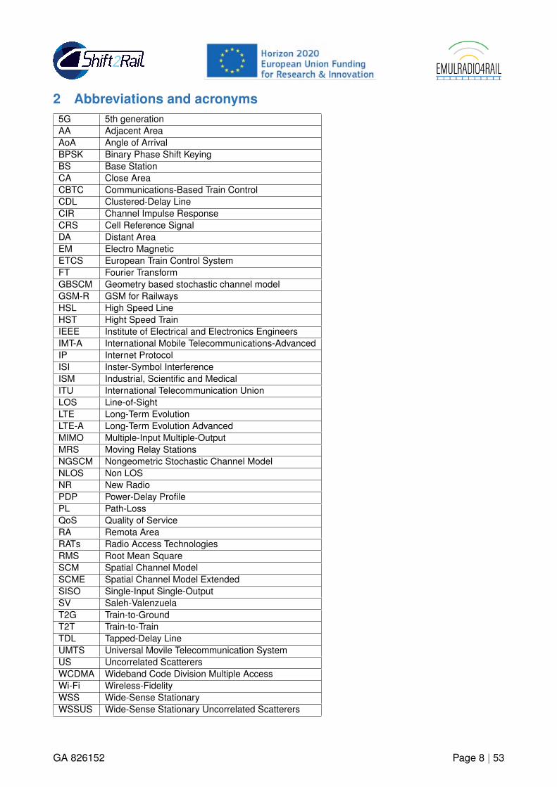
2 Abbreviations and acronyms5G 5th generationAA Adjacent AreaAoA Angle of ArrivalBPSK Binary Phase Shift KeyingBS Base StationCA Close AreaCBTC Communications-Based Train ControlCDL Clustered-Delay LineCIR Channel Impulse ResponseCRS Cell Reference SignalDA Distant AreaEM Electro MagneticETCS European Train Control SystemFT Fourier TransformGBSCM Geometry based stochastic channel modelGSM-R GSM for RailwaysHSL High Speed LineHST Hight Speed TrainIEEE Institute of Electrical and Electronics EngineersIMT-A International Mobile Telecommunications-AdvancedIP Internet ProtocolISI Inster-Symbol InterferenceISM Industrial, Scientific and MedicalITU International Telecommunication UnionLOS Line-of-SightLTE Long-Term EvolutionLTE-A Long-Term Evolution AdvancedMIMO Multiple-Input Multiple-OutputMRS Moving Relay StationsNGSCM Nongeometric Stochastic Channel ModelNLOS Non LOSNR New RadioPDP Power-Delay ProfilePL Path-LossQoS Quality of ServiceRA Remota AreaRATs Radio Access TechnologiesRMS Root Mean SquareSCM Spatial Channel ModelSCME Spatial Channel Model ExtendedSISO Single-Input Single-OutputSV Saleh-ValenzuelaT2G Train-to-GroundT2T Train-to-TrainTDL Tapped-Delay LineUMTS Universal Movile Telecommunication SystemUS Uncorrelated ScatterersWCDMA Wideband Code Division Multiple AccessWi-Fi Wireless-FidelityWSS Wide-Sense StationaryWSSUS Wide-Sense Stationary Uncorrelated Scatterers

GA 826152 | 53

ii

“output” — 2020/1/2 — 20:41 — page 9 — #9 ii

ii

ii

3 BackgroundThe present document constitutes the Deliverable D1.3 ”Characterization of the railway environment:channel models and general characteristics” in the framework of the EMULRADIO4RAIL project (GA826152), WP1/Task 1.3. This Deliverable follows an internal document (Milestone 2), which includedthe preliminary cut of channel models and also some premises to start the discussion in order toagree on the criterion to choose the final ones.

This characterization will be considered as a basis to build channel models as well as otherrepresentative characteristics for the railway applications and scenarios considered in the emulationplatform. Once the railway scenarios have been identified (see D1.1 [19] as well as the sources ofperturbations to be considered (in the internal milestone 2, plus in D1.2 [20], it is needed to go tothe literature in order to retrieve suitable channel models for all these physical layer aspects to beintroduced in the platform.

GA 826152 | 53

ii

“output” — 2020/1/2 — 20:41 — page 10 — #10 ii

ii

ii

4 ObjectivesThis document has been prepared to identify a set of suitable radio channel models for the differentrailway scenarios to be emulated in the Emulradio4rail platform. These scenarios are: tunnel, rural,cuttings, viaducts and hilly. For each of them we reference all the channel models found in the liter-ature, plus the information provided for each one of them (unfortunately, this information very oftenis not complete in terms of required knowledge such as Doppler, number of taps, etc.). Then, aftera detailed literature survey, we introduce a methodology to pick up the most suitable railway modelsto be emulated in accordance with the technical potentialities of the channel emulators considered inthe project. Finally, the final set of selected models is given.

Moreover, in order to provide some context for this deliverable, a section describing the mostrelevant topics on physical layer modelling (i.e. ’channel modelling’) is included in this Deliverable aswell. This deliverable provides a complete description of following topics:

• A complete description of the radio channel models to give a solid basis to understand the Stateof Art,

• An exhaustive state of the art made with a large literature survey on railway channel models

• The methodology followed to retrieve the radio channel models that are most suitable for theemulation platform.

• The description of the chosen models. This task had input from T1.1 (railway scenarios) andT1.2 (degraded situations) and has been an input for both T2.1 and T2.2.

GA 826152 | 53

ii

“output” — 2020/1/2 — 20:41 — page 11 — #11 ii

ii

ii

5 ContextIn this section both inputs for this task 1.3 are explained: railway scenarios (from T1.1, which wasreleased in Deliverable D1.1 [19]) and the perturbations to be introduced in the platform (from T1.2and Deliverable D1.2 [20], which will be released at the same time as this Deliverable).

5.1 Railway scenarios (input from T1.1)The first task within this Project was focused on the definition of the application layer requirementsfor Communication systems in railway environments. Therefore, a description of both the differentrailway scenarios to be covered (high-speed, urban, regional, etc.) and the services (CBTC, videosurveillance, ETCS, etc.) was provided. Moreover, some data traffic models for these communicationservices, IP-layer parameters, QoS definition and quality metrics were identified as well.

In terms of the impact on other tasks, the main outcome from task 1.1 was the identification ofscenarios and services to be emulated in the platform. Regarding the scenarios with physical-layerimpact, we decided to include the following:

• Tunnel

• Rural

• Cutting

• Viaducts

• Hilly

Obviously, tunnels are a vital scenario for subways and for mainline and high-speed but on alesser extent. Cuttings and viaducts are essential in modern high-speed lines which tend to be builtavoiding steep ramps and strong curves. Finally, both rural and hilly should be considered as basicscenarios on both main lines and high-speed lines.

It is important to note here that due to the fact that satellite bearer will be emulated only at IPlevel, this report will not detail satellite channel models.

5.2 Perturbations to be introduced (input from T1.2)Potential sources of degradation of the radio links on railway scenarios and a quantification of theirimpact are analyzed in D1.2 report [20]. This includes EM interferences, network interferences (in-terference induced by other communication networks using the same or adjacent frequencies), non-intentional EM interference sources (the most significant being transient EM interferences producedby the catenary-pantograph contact loss) and intentional EM interferences (produced by jammers onboard of the train or on the track side). These perturbations models will be added to the radio channelmodels in the channel emulators as described in [20], [18] and [21].

Once the detailed characterization of all of them and the study on their impact, a decision wasmade on which one of them were to be included in the emulation platform. Finally, we identified threeperturbations:

• Network interference in the ISM band,

• Sliding contact between the pantograph and the catenary,

• Illegal jamming.

GA 826152 | 53

ii

“output” — 2020/1/2 — 20:41 — page 12 — #12 ii

ii

ii

6 Mobile radio propagation generalities and modelling6.1 Introduction

This chapter will present the main characteristics of the mobile radio channel. We will introduce themain parameters that allow to characterize the radio channel and that will be considered later forchannel emulation. The last section is about multipath channel modelling. We will introduce thechannel impulse response.

6.2 Main characteristics of the mobile radio channel

The mobile radio channel places fundamental limits on the performance of a mobile communicationsystem. Compared to predictable and stationary wired channels, mobile radio channels are extremelyrandom. This section explains the main phenomena that we will have to take into account in this work.The main references considered are [22],[23],[24].

6.2.1 Multipath

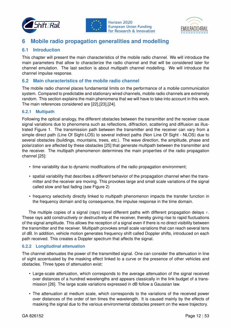
Following the optical analogy, the different obstacles between the transmitter and the receiver causesignal variations due to phenomena such as reflections, diffraction, scattering and diffusion as illus-trated Figure 1. The transmission path between the transmitter and the receiver can vary from asimple direct path (Line Of Sight-LOS) to several indirect paths (Non Line Of Sight - NLOS) due toseveral obstacles (buildings, mountains, trees, etc.). The wave direction, the amplitude, phase andpolarization are affected by these obstacles [25] that generate multipath between the transmitter andthe receiver. The multipath phenomenon determines the main properties of the radio propagationchannel [25]:

• time variability due to dynamic modifications of the radio propagation environment;

• spatial variability that describes a different behavior of the propagation channel when the trans-mitter and the receiver are moving. This provokes large and small scale variations of the signalcalled slow and fast fading (see Figure 2)

• frequency selectivity directly linked to multipath phenomenon impacts the transfer function inthe frequency domain and by consequence, the impulse response in the time domain.

The multiple copies of a signal (rays) travel different paths with different propagation delays τ .These rays add constructively or destructively at the receiver, thereby giving rise to rapid fluctuationsof the signal amplitude. This allows the reception of a signal even if there is no direct visibility betweenthe transmitter and the receiver. Multipath provokes small scale variations that can reach several tensof dB. In addition, vehicle motion generates frequency shift called Doppler shifts, introduced on eachpath received. This creates a Doppler spectrum that affects the signal.

6.2.2 Longitudinal attenuation

The channel attenuates the power of the transmitted signal. One can consider the attenuation in lineof sight accentuated by the masking effect linked to a curve or the presence of other vehicles andobstacles. Three types of attenuation exist:

• Large-scale attenuation, which corresponds to the average attenuation of the signal receivedover distances of a hundred wavelengths and appears classically in the link budget of a trans-mission [26]. The large scale variations expressed in dB follow a Gaussian law.

• The attenuation at medium scale, which corresponds to the variations of the received powerover distances of the order of ten times the wavelength. It is caused mainly by the effects ofmasking the signal due to the various environmental obstacles present on the wave trajectory.

GA 826152 | 53

ii

“output” — 2020/1/2 — 20:41 — page 13 — #13 ii

ii

ii

Figure 1: Illustration of multipath phenomenon

• The small-scale attenuation that corresponds to the fluctuations of the signal received overdistances of the order of the wavelength. These variations are due to the physical phenomenonof multiple paths [27]. The well known small-scale variation laws are: Rayleigh for non line ofsight reception, Rice for line of sight reception [24].

Figure 2: Illustration of slow and fast fading

6.2.3 Delay spread

The variation of the delay due to multipath can be statistically characterized. The delay spreadcorresponds to the variations of the delay around the mean value. The parameters that can be usedto characterize the path delays in the channel are [28]:

• First-Arrival delay,

• RMS delay or deay spread,

• Mean excess delay,

• Maximal excess delay.

.

GA 826152 | 53

ii

“output” — 2020/1/2 — 20:41 — page 14 — #14 ii

ii

ii

These parameters are illustrated in Figure 3 that represents the so called Power Delay ProfilePh(τ) at a given position, which represents the average power associated with a given multipathdelay when a pulse is sent into the channel.

Figure 3: Illustration of Power delay profile measured

• The First-Arrival Delay (τA) is a time delay corresponding to the arrival of the first transmittedsignal at the receiver. It is usually measured at the receiver. This delay is set by the minimumpossible propagation path delay from the transmitter to the receiver. It serves as a reference,and all delay measurements are made relative to it. Any measured delay longer than thisreference delay is called an excess delay.

• The RMS Delay (τrms) is referred to the second order moment (variance) of the mean excessdelay.

• The Maximum Excess Delay (τm), also called Maximum Delay Spread, denoted as τm, is therelative time difference between the first signal component arriving at the receiver to the lastcomponent whose power level is above some threshold. The RMS Delay spread is typicallydefined as (1):

τrms =√∑

k P (τk)(τk − τ)2∑k P (τk)

(1)

where

τ =√∑

k P (τk)τk∑k P (τk)

(2)

where P (τk) represents the power associated to the kth path. If the given Power Delay Profilevalues are continuous in terms of time delays, we replace the summation with integral and in-tegrate it with respect to dτ .

In the frequency domain, the channel coherence bandwidth is defined as Bc is proportional to1/τrms as a dual variable of τrms. Bc corresponds to the frequency band on which the transfer func-tion of the channel can be considered as constant. On this frequency band, the spectral componentsof the signal are affected similarly. Both parameters are used to characterize frequency selectivity ofa channel. When the signal bandwidth Bs is much lower than the coherence bandwidth Bs Bc, thechannel is considered as non selective in frequency. On the contrary, the channel is frequency selec-tive. This resul inter symbol interferences (ISI). Channel selectivity impacts the system performance.

GA 826152 | 53

ii

“output” — 2020/1/2 — 20:41 — page 15 — #15 ii

ii

ii

6.2.4 Doppler effect

Doppler effect refers to the shift of frequency of any radio signal due to the mobility. The Doppler shiftfd for the ith path is proportional to the mobile speed v and the carrier frequency fc. The Dopplerequation for one ray is given by equation (3) [29]:

fdi= fc

v

C. cos (βi) (3)

where fc is the carrier frequency, C is the speed of light, v is the speed of the mobile, βi is thearrival angle of the ith path with the speed vector of the mobile.

Each path experiences a Doppler shift, then depending of the angle of arrival distribution, aDoppler spectrum is observed. If the angle of arrival are distributed between [−π,+π] the Dopplerspectrum can be expressed by equation (4) [30] and represented by Figure 4.

S(f) =

σ2

πfd. 1√

1− ffd

2, where− fd ≤ f ≤ +fd

0, otherwise(4)

where σ2 is the variance of the signal and fd the maximal Doppler spread.

This Doppler spectrum is also known as Classical Doppler spectrum or Jakes Doppler spectrumillustrated in Figure 4. Depending on the distribution of the angles of arrival due to the environmentbut also due to the characteristics of receiving antenna, various Doppler spectrum shapes exist. Themost well known are the Flat Doppler spectrum, the Gaussian and the Rice Doppler spectrum.

The time varying nature of the frequency dispersiveness of the channel in the time domain ischaracterized by the coherence time Tc which is inversely proportional to the Doppler spread.

Figure 4: Representation of the Classic Doppler spectrum [2]

The Flat Doppler spectrum can be expressed by equation (5) [30] and represented by figure 5.

S(f) = 12fd

, fd 6= 0 (5)

The Gaussian Doppler spectrum can be expressed by equation (6) [30] and represented by figure6.

GA 826152 | 53

ii

“output” — 2020/1/2 — 20:41 — page 16 — #16 ii

ii

ii

Figure 5: Representation of the Flat Doppler spectrum

S(f) =

1√2πσ2 exp(

f2

2σ2 ), |f | ≤ fd0, |f | > fd

(6)

where σ = σg.fd with σg the standard deviation of the Gaussian classical function.

Figure 6: Representation of the Gaussian Doppler spectrum

The 3GPP-Rice Doppler spectrum can be expressed by equation (7) [30] and represented byfigure 7.

S(f) =

0.412πfd

. 1√1+109−( f

fd)2

+ 0.91δ(f − 0.7fd), |f | ≤ fd

0, |f | > fd

(7)

GA 826152 | 53

ii

“output” — 2020/1/2 — 20:41 — page 17 — #17 ii

ii

ii

Figure 7: Representation of the Rice Doppler spectrum

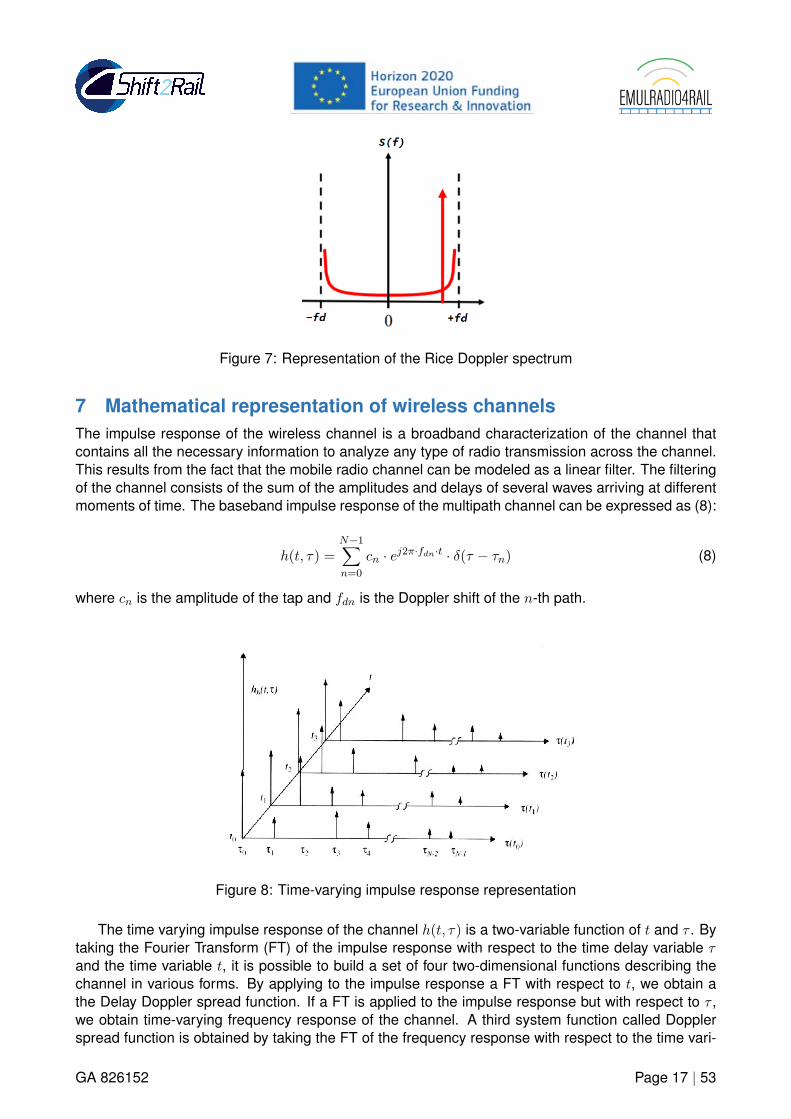
7 Mathematical representation of wireless channelsThe impulse response of the wireless channel is a broadband characterization of the channel thatcontains all the necessary information to analyze any type of radio transmission across the channel.This results from the fact that the mobile radio channel can be modeled as a linear filter. The filteringof the channel consists of the sum of the amplitudes and delays of several waves arriving at differentmoments of time. The baseband impulse response of the multipath channel can be expressed as (8):

h(t, τ) =N−1∑n=0

cn · ej2π·fdn·t · δ(τ − τn) (8)

where cn is the amplitude of the tap and fdn is the Doppler shift of the n-th path.

Figure 8: Time-varying impulse response representation

The time varying impulse response of the channel h(t, τ) is a two-variable function of t and τ . Bytaking the Fourier Transform (FT) of the impulse response with respect to the time delay variable τand the time variable t, it is possible to build a set of four two-dimensional functions describing thechannel in various forms. By applying to the impulse response a FT with respect to t, we obtain athe Delay Doppler spread function. If a FT is applied to the impulse response but with respect to τ ,we obtain time-varying frequency response of the channel. A third system function called Dopplerspread function is obtained by taking the FT of the frequency response with respect to the time vari-

GA 826152 | 53

ii

“output” — 2020/1/2 — 20:41 — page 18 — #18 ii

ii

ii

able t.

The four system functions are known as Bellofuntions [31]. h(t, τ) is the Impulse response,H(t, f) the Transfer function or frequency response, S(τ, fd) the Delay Doppler spread function andD(f, fd) the Doppler spread function illustrated in Figure 9.

Figure 9: Bello functions

In order to characterize the stochastic process, the autocorrelation function (ACF) can be used.An autocorrelation function describes the similarity between a system function with delayed copy ofitself over successive time intervals. The autocorrelation function of the channel impulse response isobtained by (9):

Rh(t, t′; τ, τ ′) = Eh(t, τ)h∗(t′, τ ′) (9)

where t and t′ are time variables, τ and τ ′ are time delay variables, ∗ indicates the complex con-jugate and E is the expectation value of the ensemble process.

From a general point of view, the output of the channel y(t) can be expressed as the convolutionof the complex channel impulse response and the input x(t) [32] as (10):

r(t) = h(t, τ) ∗ s(t) +N(t) (10)

where r(t) and s(t) denote the output signal and the input signal respectively. N(t) is a whiteGaussian noise.

7.1 Representation of the MIMO channel

A MIMO system is defined by the number of antennas at transmitter Nt side and the number ofantennas at receiver side Nr. The classical representation of a MIMO channel relies on a chan-nel description based on Nr x Nt independent SISO channels modeled with the H matrix. Theequivalent diagonal matrix system allows expressing the channel as the superposition of severaleigen-decorrelation channels. As recall in [33], it was demonstrated that the MIMO radio propaga-tion channel is constituted of the superposition of several independent sub channels each carrying afraction of the transmitted signal [9], [34]. The MIMO channel appears as a linear application of theemitted signal X towards the received signal Y. The singular value decomposition [35] of the H matrixallows the diagonalization of the linear system of equations. This singular value decomposition allowsthe diagonalization of the MIMO matrix system. The MIMO propagation channel can be modeled intwo different ways. The first approach is to represent the MIMO propagation channel by a matrix ofimpulse responses containing all the impulse responses between each SISO link in the system.

GA 826152 | 53

ii

“output” — 2020/1/2 — 20:41 — page 19 — #19 ii

ii

ii

When delays dispersion is greater than the symbol duration of the MIMO system, the impulseresponse of the channel are represented by several samples of K main propagation paths. Thechannel is large bandwidth. The impulse response matrix H (t) is expressed as the sum K channelmatrices Hk each shifted of a delay τk as indicated in the following equation.

H (t) =K∑k=1

Hk · δ (t− τk) (11)

where H (t) is the channel matrix (Nr ×Nt) modelling the channel characterised byK main pathsand Hk is the matrix of (nr × nt) complex coefficients at instant τk such as (12) :

Hk =

hk11 hk12 · · · hk1nt

hk21 hk22 · · · hk2nt

· · · · · · · · · · · ·hknr1 hknr2 · · · hknrnt

(12)

When the delays dispersion is very low compared to the symbol duration, the channel is con-sidered as narrow band or non selective in frequency. The MIMO channel is perfectly described bythe (Nr ×Nt) channel matrix H = H1 with complex coefficients in narrow band. Each complex coef-ficient represents the sum of all the received paths for a given position of both transmitter and receiver.

For a Nr × Nt MIMO system, where Nr and Nt are respectively the number of antennas at thetransmitter and the receiver. The time variant MIMO matrix is defined by the equation (13):

H(t, τ) =

h11(t, τ) h12(t, τ) . . . h1n(t, τ)h21(t, τ) h22(t, τ) . . . h2n(t, τ)

......

. . ....

hm1(t, τ) hm2(t, τ) . . . hmn(t, τ)

(13)

Where hmn(t, τ) is the SISO impulse response between the mth transmitter antenna and the nth

receiver antenna.

The MIMO impulse response matrix, equation (13) can be used as a formalism of a MIMO input-output system between the transmitted signal vector x(t) of size Nt and the vector of output signalsy(t) of size Nr as follows:

y(t) =∫TH(t, τ)x(t− τ)dτ + b(t) (14)

Where b(t) is the noise and interferences.

The second way to model the MIMO propagation channel is to represent the propagation channelby its doubly directional impulse response [36], [24] between the transmitter and the receiver. Thedoubly directional impulse response defined by Steinbauer and Molisch corresponds to the impulseresponse defined as follows.

In the case of MIMO, several antennas are used at the transmitter and the receiver to exploit thespatial diversity of the propagation channel. [37] shows that the Fourier analysis makes it possible todemonstrate the duality between space and wave in the same way as it exists between the time andfrequency spaces [38]. The wave vector corresponds to the direction of propagation of a path. As aresult, the impulse response of a MIMO channel between a pair of transceiver-receiver antennas canbe written as:

GA 826152 | 53

ii

“output” — 2020/1/2 — 20:41 — page 20 — #20 ii

ii

ii

h(t, τ,ΩBS ,ΩMS) =K−1∑k=0

αk(t)exp(−jΦk(t))δ(τ − τk(t))δ(ΩBS − ΩBS,k(t))δ(ΩMS − ΩMS,k(t)) (15)

Where ΩBS,k and ΩMS,k are the propagation directions of the kth path at the BS and MS respec-tively. Ω is a direction characterized by an azimuth angle ϕ and elevation angle θ as presented figure10.

Figure 10: Representation of azimuth and elevation angles

The polarization diversity is taken into account by decomposing the impulse response accordingto the vertical and horizontal components. The impulse response of the radio propagation channelis then a matrix containing the different states of polarization (VV, VH, HH and HV) illustrated byequation (16):

h(t, τ,ΩBS ,ΩMS) =[hV V (t, τ,ΩBS ,ΩMS) hV H(t, τ,ΩBS ,ΩMS)hHV (t, τ,ΩBS ,ΩMS) hHH(t, τ,ΩBS ,ΩMS)

](16)

The propagation channel is completely described if there are the knowledge of the complex am-plitude of each polarization states, propagation delay, direction of arrival at the BS and direction ofarrival at the MS.

7.2 Wide Sense Stationary Channel (WSSUS) [[1]

The autocorrelation function depends on four variables, and is thus a rather complicated form for thecharacterization of the channel. Further assumptions about the physics of the channel can lead toa simplification of the correlation function. The most frequently used assumptions are the so-calledWide-Sense Stationary (WSS) assumption and the Uncorrelated Scatterers (US) assumption. Amodel using both assumptions simultaneously is called a WSSUS model. This assumption is veryfrequent even though it is far from reality. This assumption considers that over short periods of time orover small spatial distances, mobile radio channels are assumed to be stationary. Physically speak-ing, WSS means that the statistical properties of the channel do not change with time. Moreover, thechannel response associated with a given multipath component of delay τ is uncorrelated with the re-sponse associated with a multipath component at a different delay τ ′ 6= τ , since the two componentsare caused by different scatterers.

GA 826152 | 53

ii

“output” — 2020/1/2 — 20:41 — page 21 — #21 ii

ii

ii

7.3 ConclusionIn this section we have described the main features of the mobile wireless radio channel. We haveintroduced the channel impulse response that is used to model the wireless channel. In the followingsection we will present some well known mobile radio channel models.

GA 826152 | 53

ii

“output” — 2020/1/2 — 20:41 — page 22 — #22 ii

ii

ii

8 Mobile Radio channel models8.1 IntroductionThe evaluation of wireless system performances requires to model the wireless channel. The mod-els are generally based on mathematical representation of the impulse response of the channel.This topic is widely treated in the literature and the channel models are changing in relation with theincreasing complexity of the communication systems. More and more parameters are taken into ac-count in order to model radio channels as closed as possible to real channels. From a very generalpoint of view, we can distinguish analytical, geometric and non geometric channel models.

Geometry based stochastic channel model (GBSCM) is a model that describes the statistics ofthe channel using a geometry representation of the physical environment and more particularly, ageometrical statistical description of the scatters. The GBSCM chooses scholastically the localiza-tion of scatterers following a certain distribution probability [39]. It exists three common techniquesnamed: One Ring, Two Rings and Distributed scattering. The GBSCM is used by different organiza-tions (3GPP, ITU, European projects) to model the channel in different scenarios. We can mentionthe spatial channel model (SCM) [40], [41], its extension (SCME) [42], WINNER [43], [7], [44], ITU-Advanced [10] and METIS [45].

The use of these types of radio channel models in the Emulradio4rail platform required that allthe geometric parameters can be implemented in the channel emulators. As we already explained inD2.1 [18] and D3.1 [21], the channel emulators used in the project can only implement the so called”Tapped Delay Line models”. Consequently, in this deliverable, we will focus on the most simpleones, the non geometric stochastic channel model with the description of the Tapped Delay Line(TDL) channel model.

8.2 Non-Geometric Stochastic Channel Model

8.2.1 Introduction

A nongeometric stochastic channel model (NGSCM) is a model, which describes the paths betweenthe transmitter and the receiver by statistical parameters. The geometry of the physical scenario isnot taken in account. Two kinds of NGSCM can be found in the literature, the Tapped Delay Line(TDL) model that represents the channel by the definition of different paths in time/delay domain,and the Saleh-Valenzuela model, which represents the channel by a definition of clusters of paths intime/delay and angular domain, which is an extension of the TDL model. We will present the TDLmodel.

8.2.2 Tapped Delay Line channel model

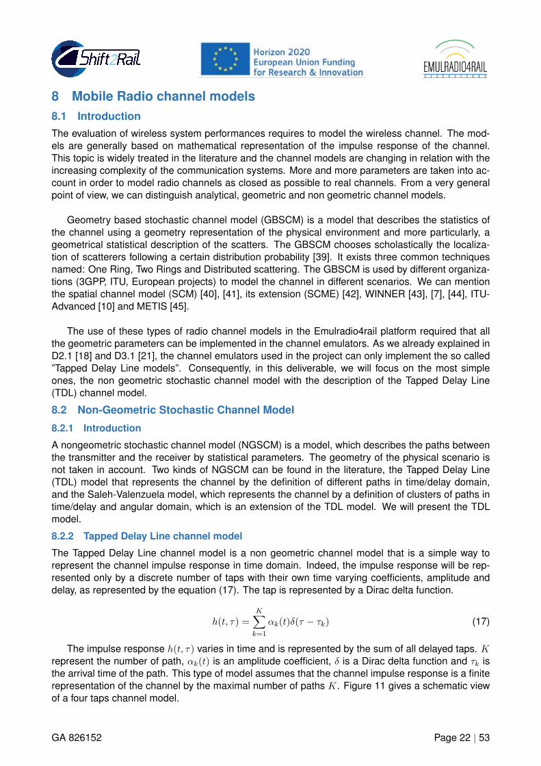
The Tapped Delay Line channel model is a non geometric channel model that is a simple way torepresent the channel impulse response in time domain. Indeed, the impulse response will be rep-resented only by a discrete number of taps with their own time varying coefficients, amplitude anddelay, as represented by the equation (17). The tap is represented by a Dirac delta function.

h(t, τ) =K∑k=1

αk(t)δ(τ − τk) (17)

The impulse response h(t, τ) varies in time and is represented by the sum of all delayed taps. Krepresent the number of path, αk(t) is an amplitude coefficient, δ is a Dirac delta function and τk isthe arrival time of the path. This type of model assumes that the channel impulse response is a finiterepresentation of the channel by the maximal number of paths K. Figure 11 gives a schematic viewof a four taps channel model.

GA 826152 | 53

ii

“output” — 2020/1/2 — 20:41 — page 23 — #23 ii

ii

ii

Figure 11: TDL representation of four taps

The resolution between two paths is limited by the bandwidth of the system as follows: δt = 1W

where δt is the maximal time resolution and W the bandwidth. For example, with a bandwidth equalto 20 MHz, the maximal time resolution is 50 ns. It is then possible to define a TDL with tap delayscorresponding to the sampling times. The associated weight is then a sum of the complex path am-plitudes contributing to the considered delay.

8.2.3 ITU models

The ITU models were developed by the IMT-2000 group to evaluate the IMT technologies like UMTS,LTE (3G) [46]. The purpose of these channels is to help system designers and network plannerswith a standard channel model to facilitate the system design and performance evaluation. The ITUmodel is used to model the time dispersion of the time variant wireless propagation channel as aTapped Delay Line model. A set of four channel models is defined: Indoor office, Outdoor to indoorpedestrian, vehicular, Mixed-cell pedestrian/vehicular. The models are constructed to simulate themulti-path fading of a SISO channel with a 5 MHz of bandwidth at 2 GHz.

The multipath fading is modeled as a TDL with six taps with non uniform delay distribution. Eachtap associates an amplitude characterized by a distribution (Rician with a K-factor > 0, or Rayleighwith K-factor= 0) and the maximal Doppler frequency. The recommendation specifies two differentdelay spreads for each test environment: low delay spread represented by ’A’, and medium delayspread represented by ’B’. Each profile has a probability to emerge along time following the descrip-tion in table 1. A more complex MIMO channel model based on Cluster Delay Line is given in [10].

Test environmentChannel A Channel B

rms (ms) P (%) rms (ms) P (%)Indoor Office 35 50 100 45

Outdoor to indoor and pedestrian 45 40 750 55Vehicular - High antenna 370 40 4000 5

Table 1: Probability of occurrence P in % for low delay spread and medium delay spread for eachITU scenarios [10]

The key parameters to describe each propagation scenario have to include: time delay spread,path loos and exceed path loss, shadow fading, multipath fading characteristics (Doppler spectrum),operating radio frequency.

The path loss model for vehicular environment is given by equation (18). The slow variation isconsidered as a log-normal distribution. This equation is given for urban and suburban area with anearly uniform height for buildings.

L = 40.(1− 4× 10−3∆hb).log10R− 18log10∆hb + 21log10f + 80 (18)

GA 826152 | 53

ii

“output” — 2020/1/2 — 20:41 — page 24 — #24 ii

ii

ii

where R is the distance between base station and mobile station in kilometer, f is the carrierfrequency equal to 2 GHz and ∆hb is the base station antenna height in meters. The model is validfor ∆hb ranging from 0 to 50 m.

The slow fading over the distance implies that the adjacent fading values are correlated. Thenormalized autocorrelation function is approximated by an exponential function [47] as indicated byequation (19).

R(∆x) = exp(−|∆x|dcorr

ln2) (19)

where ∆x is the distance between fading and dcorr is the decorrelation length.

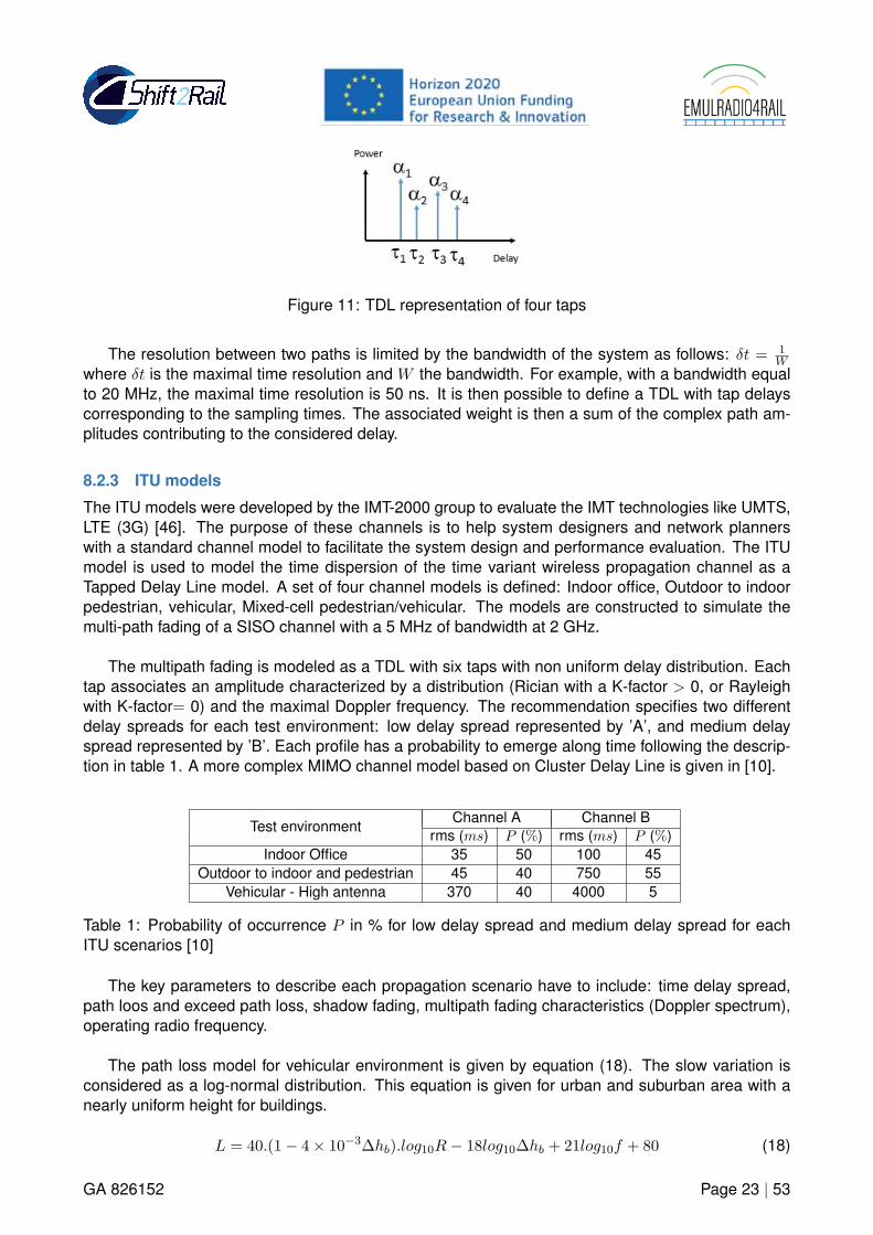
The scenario called Vehicular B is defined for a speed up to 120 km/h with a six taps TDL channelmodel. It is characterized by the number of taps, time delay relative to the first tap, average powerrelative to the strongest tap and Doppler spectrum as presented in the table 2.

TapChannel A Channel B

Doppler spectrumRelative delay (ns) Average power (dB) Relative delay (ns) Average power (dB)

1 0 0.0 0 -2.5 Clasic2 310 -1.0 300 0 Clasic3 710 -9.0 8 900 -12.8 Clasic4 1090 -10.0 12 900 -10.0 Clasic5 1730 -15.0 17 100 -25.2 Classic6 2510 -20.0 20 000 -16.0 Classic

Table 2: ITU channel model for vehicular-A (30 km/h) and vehicular-B (120 km/h) scenarios [10]

8.2.4 Saleh-Valenzuela channel model

The Saleh-Valenzuela (SV) is originally developed for SISO wideband channel [48] and was furtherextended to MIMO system by including angle of arrival (AoA) [49]. The SV channel model is similar tothe TDL model in term of using path representation with delay and magnitude identification. The SVchannel model uses a definition of the so-called cluster representation. A cluster is a group of pathsthat comes from the same scatterer. This model defines the CIR of the channel with the followingequation (20):

h(t, τ) =C−1∑c=1

K−1∑k=1

βkcexp(jφkc)δ(t− Tc − τkc) (20)

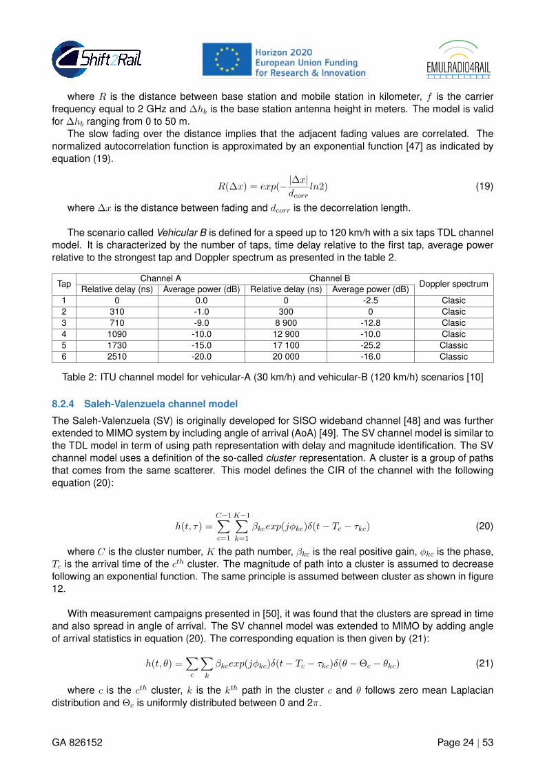
where C is the cluster number, K the path number, βkc is the real positive gain, φkc is the phase,Tc is the arrival time of the cth cluster. The magnitude of path into a cluster is assumed to decreasefollowing an exponential function. The same principle is assumed between cluster as shown in figure12.

With measurement campaigns presented in [50], it was found that the clusters are spread in timeand also spread in angle of arrival. The SV channel model was extended to MIMO by adding angleof arrival statistics in equation (20). The corresponding equation is then given by (21):

h(t, θ) =∑c

∑k

βkcexp(jφkc)δ(t− Tc − τkc)δ(θ −Θc − θkc) (21)

where c is the cth cluster, k is the kth path in the cluster c and θ follows zero mean Laplaciandistribution and Θc is uniformly distributed between 0 and 2π.

GA 826152 | 53

ii

“output” — 2020/1/2 — 20:41 — page 25 — #25 ii

ii

ii

Figure 12: Saleh-Valenzuela representation following exponential decrease [3]

9 Radio channel models based on measurements and simulations intypical railway environments

9.1 IntroductionWith the development of wireless communications in the railway domain, the development of channelmodels for railways is a very active field in a small community of researchers in the world. The authorsgenerally considered Train to Ground (T2G), Train to Train (T2T) and intra-train communications forhigh speed train environments and also tunnels in the case of metro. The literature analysis showsthat the majority of the papers are dealing with radio propagation models and they mainly presentnarrow band parameters such as path loss, fading statistics, angle distribution statistics and some-times the delays and RMS delays distribution. We have also identified papers that present Tap delayLine and Cluster Delay lines models in different railway environments.

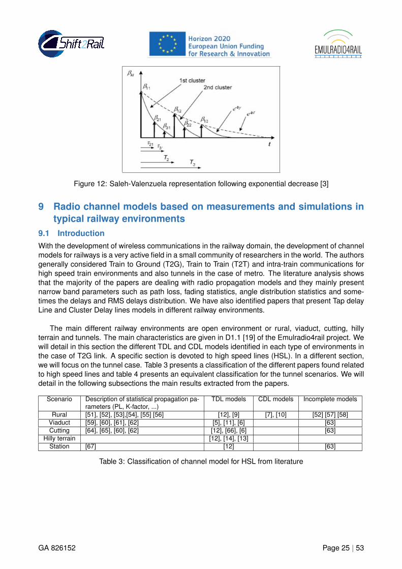
The main different railway environments are open environment or rural, viaduct, cutting, hillyterrain and tunnels. The main characteristics are given in D1.1 [19] of the Emulradio4rail project. Wewill detail in this section the different TDL and CDL models identified in each type of environments inthe case of T2G link. A specific section is devoted to high speed lines (HSL). In a different section,we will focus on the tunnel case. Table 3 presents a classification of the different papers found relatedto high speed lines and table 4 presents an equivalent classification for the tunnel scenarios. We willdetail in the following subsections the main results extracted from the papers.

Scenario Description of statistical propagation pa-rameters (PL, K-factor, ...)

TDL models CDL models Incomplete models

Rural [51], [52], [53],[54], [55] [56] [12], [9] [7], [10] [52] [57] [58]Viaduct [59], [60], [61], [62] [5], [11], [6] [63]Cutting [64], [65], [60], [62] [12], [66], [6] [63]

Hilly terrain [12], [14], [13]Station [67] [12] [63]

Table 3: Classification of channel model for HSL from literature

GA 826152 | 53

ii

“output” — 2020/1/2 — 20:41 — page 26 — #26 ii

ii

ii

Scenario Description of statistical propagation pa-rameters (PL, K-factor, AoA, AoD, ...)

IncompleteSaleh-Valenzuelamodel

Kronecker We-ichselbergermodel

CDL model

Tunnel [68], [69], [70], [71], [72], [73], [74], [75],[76], [77], [78], [79], [80], [81], [82], [83],[84], [85], [86], [86], [87]

[88] [89] [8]

Table 4: Classification of channel model for HSL from literature

9.2 Channel models obtained with measurements and simulations along high speedlines

9.2.1 Introduction

For some years now, journal papers presenting results of channel measurements along high-speedlines are quite numerous with the development of high speed train (HST) particularly in China. Theseenvironments are built to allow trains to run generally up to 350 km/h. Such a speed involves a lot ofconstraints for the measurements such as: large Doppler spread and fast variations of the channelsparameters. A HST can, on a same line, pass over several scenarios. The high-speed environmentcan be classified into different scenarios: open space, viaduct, cutting, station and large tunnel [4].The tunnel scenario will be considered in a following section. It is important to notice that there is nota lot of published papers referring to train-to-ground measurements along high speed line in Europe,the majority of the papers present results obtained along HSL in China.

As mentioned before, most of the results in the literature present the statistical properties of nar-row band channel characteristics such as Path Loss and K-factor and distributions of angle of arrivalor departure of the paths. In [51], [52], [12], [53], [54], [55] and [56], authors present results for variousrural railway scenarios. A description of the radio propagation characteristics is given in [60], [59],[61] and [62] for viaduct scenario. The radio propagation characteristics in different cutting scenariosare described in [64], [65], [60] and [62]. An analysis of path loss and K-factor is performed in [67] fora station scenario.

In this report we decided to focus on wide band channel models that can be used for system eval-uation, ie models that provide a description of the complex impulse response of the channel. SeveralTDL channel models are considered in [9] for rural scenario and also two CDL channel models in [7]and [10]. [5], [11] and [6] treated the case of viaduct scenario. [12], [66] and [6] deal with cutting sce-nario. [12], [14] and [13] present results for hilly terrain scenario and [12] for station scenario. We willpresent all these channel models starting with the TDL models then we will describe the CDL models.

9.2.2 Train to Ground Tapped Delay line channel model for high speed line scenarios

In [4], the high speed train geographical environment is divided in sub environments as illustrated infigure 13. We will follow this classification for the channel models.

Open space scenarioThis scenario is the most common HSL environment in China. If we consider T2G communica-

tions, the base stations are generally distributed along the tracks. Consequently, the LoS componentis generally dominant between the transmitter and the receiver. As the distance between the trans-mitter and the receiver increases, the impact of the scatters becomes important and causes manymulti-paths.

GA 826152 | 53

ii

“output” — 2020/1/2 — 20:41 — page 27 — #27 ii

ii

ii

Figure 13: Classification of High Speed Train environments [4]

In [9], the authors present a measurement campaign in China between Beijing South RailwayStation and Wuqing Station over 30 km. They considered public LTE FDD transmission. The speedof train is equal to 300 km/h. They use a NI-USRP 2952 (National Instrument-Universal SoftwareRadio Peripheral) board as receiver to get channel information from LTE standard signal. The mea-surements are performed with SISO antenna configuration at 1.85 GHz with 20 MHz bandwidth and30.72 MS/s sampling rate. Due to the bandwidth, the maximal delay resolution is equal to 0.06 µs.The maximal time delay which can be calculated is 11 µs because of the 90 kHz between two suc-cessive cell-specific reference signal (CRS). The receive antenna is located inside the train. Theauthors are able to define a two taps model for this open area scenario represented in the table 5.The characteristics of the antennas are not given.

Parameters ValueCenter frequency 1.85 GHz

Bandwidth 20 MHzSpeed 300 km/h

Antenna Configuration SISOPath Delay (µs) Relative power (dB)

LOS path 0.2 -35.10Second path 1.2 -49.60

Table 5: Two taps model for open area scenario at 300 km/h [9]

Viaduct scenariosIn viaduct scenarios the LoS component is dominant and the scatters have a minor impact on

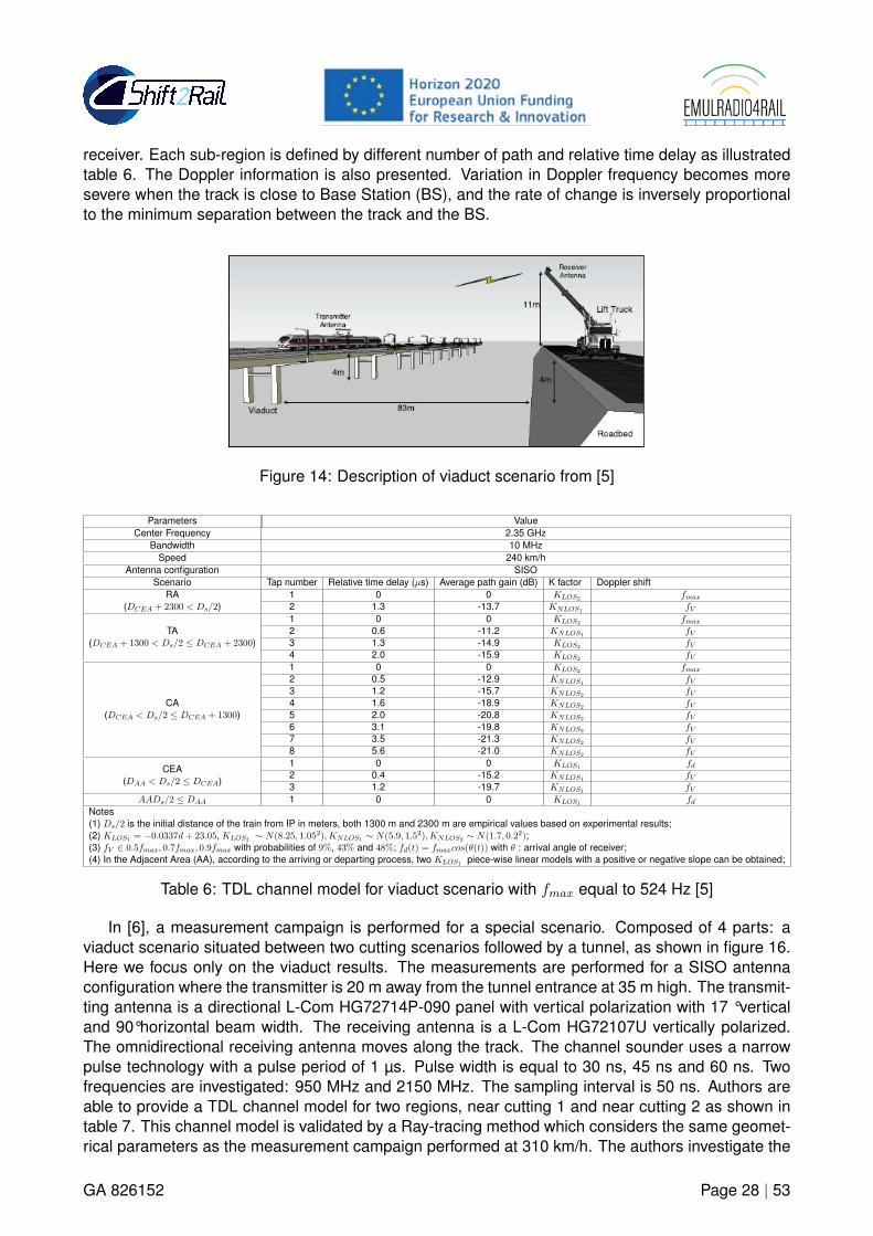
the receiver. In [5] a measurement campaign is performed in a viaduct scenario in China on Beijing-Tianjin HSL. The transmitter antenna is 3 m above the rail, on the top of the train and the receiveris located on the road at 83 m far from the viaduct as presented in figure 15. The antennas con-figuration is SISO with a wide band vertical-polarized Sencity Rail Antenna HUBER+SUHNER [90]transmit antenna and a dipole for the receiver antenna. The train speed is equal to 240 km/h and thereceiver is an Elektrobit Propsound TM Channel Sounder working at 2.35 GHz with 10 MHz band-width. A direct sequence spread spectrum signal is used to extract the CIR with a length of 127 bits.Two Rubidium clocks are used to synchronize the transmitter and receiver. Authors divide the envi-ronment into five sub-regions related to the intersection point (IP) between the transmitting pylon andthe track. The sub regions are defined depending on the average number of taps obtained in eachsub region. They set up five corresponding TDL channel models for the viaduct scenario. The fiveareas are Remote Area (RA) with two paths, Toward Area (TA) with four paths, Close Area (CA) witheight paths, Closer Area (CEA) with three paths and Arrival Area (AA) into one tap. The number ofpath depends of resolvable multi-path components over the distance between the transmitter to the

GA 826152 | 53

ii

“output” — 2020/1/2 — 20:41 — page 28 — #28 ii

ii

ii

receiver. Each sub-region is defined by different number of path and relative time delay as illustratedtable 6. The Doppler information is also presented. Variation in Doppler frequency becomes moresevere when the track is close to Base Station (BS), and the rate of change is inversely proportionalto the minimum separation between the track and the BS.

Figure 14: Description of viaduct scenario from [5]

Parameters ValueCenter Frequency 2.35 GHz


Antenna configuration SISOScenario Tap number Relative time delay (µs) Average path gain (dB) K factor Doppler shift

RA(DCEA + 2300 < Ds/2)

1 0 0 KLOS2 fmax2 1.3 -13.7 KNLOS1 fV

TA(DCEA + 1300 < Ds/2 ≤ DCEA + 2300)

1 0 0 KLOS2 fmax2 0.6 -11.2 KNLOS1 fV3 1.3 -14.9 KLOS2 fV4 2.0 -15.9 KLOS2 fV

CA(DCEA < Ds/2 ≤ DCEA + 1300)

1 0 0 KLOS2 fmax2 0.5 -12.9 KNLOS1 fV3 1.2 -15.7 KNLOS2 fV4 1.6 -18.9 KNLOS2 fV5 2.0 -20.8 KNLOS2 fV6 3.1 -19.8 KNLOS2 fV7 3.5 -21.3 KNLOS2 fV8 5.6 -21.0 KNLOS2 fV

CEA(DAA < Ds/2 ≤ DCEA)

1 0 0 KLOS1 fd2 0.4 -15.2 KNLOS1 fV3 1.2 -19.7 KNLOS1 fV

AADs/2 ≤ DAA 1 0 0 KLOS1 fdNotes(1) Ds/2 is the initial distance of the train from IP in meters, both 1300 m and 2300 m are empirical values based on experimental results;(2) KLOS1 = −0.0337d+ 23.05, KLOS2 ∼ N(8.25, 1.052),KNLOS1 ∼ N(5.9, 1.52),KNLOS2 ∼ N(1.7, 0.22);(3) fV ∈ 0.5fmax, 0.7fmax, 0.9fmax with probabilities of 9%, 43% and 48%; fd(t) = fmaxcos(θ(t)) with θ : arrival angle of receiver;(4) In the Adjacent Area (AA), according to the arriving or departing process, two KLOS1 piece-wise linear models with a positive or negative slope can be obtained;

Table 6: TDL channel model for viaduct scenario with fmax equal to 524 Hz [5]

In [6], a measurement campaign is performed for a special scenario. Composed of 4 parts: aviaduct scenario situated between two cutting scenarios followed by a tunnel, as shown in figure 16.Here we focus only on the viaduct results. The measurements are performed for a SISO antennaconfiguration where the transmitter is 20 m away from the tunnel entrance at 35 m high. The transmit-ting antenna is a directional L-Com HG72714P-090 panel with vertical polarization with 17 °verticaland 90°horizontal beam width. The receiving antenna is a L-Com HG72107U vertically polarized.The omnidirectional receiving antenna moves along the track. The channel sounder uses a narrowpulse technology with a pulse period of 1 µs. Pulse width is equal to 30 ns, 45 ns and 60 ns. Twofrequencies are investigated: 950 MHz and 2150 MHz. The sampling interval is 50 ns. Authors areable to provide a TDL channel model for two regions, near cutting 1 and near cutting 2 as shown intable 7. This channel model is validated by a Ray-tracing method which considers the same geomet-rical parameters as the measurement campaign performed at 310 km/h. The authors investigate the

GA 826152 | 53

ii

“output” — 2020/1/2 — 20:41 — page 29 — #29 ii

ii

ii

Figure 15: A - Relative positions over the distance. The blue dashed line denotes Dmin, the bluepoint represents IP of Dmin and the rail. DAA, DCEA, DCA and DTA are the distances from IP to thecorresponding area bound, respectively. B - Schematic illustration of DCEA . [5]

correlation coefficients between delay and Doppler. For viaduct scenario the correlation coefficientequals 0.0308 and 0.0143 respectively for 950 MHz and 2150 MHz.

Figure 16: Description of viaduct scenario from [6]

In [11], another measurement campaign is performed for viaduct scenario on Harbin-Dalian HSL.The measurements are performed for a 2x2 MIMO configuration where the transmitter is 15 m awayfrom the viaduct at 40 m height. The transmit antenna is omnidirectional with 45°of vertical polar-ization with 65°and 7°vertical beam width. The receiving antennas are positioned on the roof of thetrain with a distance of 0.5λ. The sounding signal is a M-sequence with a length of 1023 using BinaryPhase Shift Keying (BPSK) modulation. The measurement campaign is performed at 2.6 GHz witha 20 MHz bandwidth. The train speed is equal to 370 km/h. Two Agilent N9020 spectrum analyzers

GA 826152 | 53

ii

“output” — 2020/1/2 — 20:41 — page 30 — #30 ii

ii

ii

Parameters ValueCenter frequency 950 MHz 2.15 GHz

Bandwidth 20 MHz 20 MHzSpeed 310 km/h 310 km/h

Antenna configuration SISO SISOScenario Delay (µs) Relative power (dB) Delay (µs) Relative power (dB)

Near cutting 10 0 0 0

108.3 -37.27 106.5 -22.95428.4 -39.6

Near cutting 20 0 0 0

89.5 -9.5 107.3 -21.46

Table 7: TDL model for viaduct scenario [6]

are used with a sampling rate of 19.53 ns. Contrary to the viaduct TDL models presented before,this model does not define sub-regions and provide a four taps delay model as described in Table 8.The mean RMS delay equals 203 ns higher than the one obtained with WINNER II channel model forLOS rural environment.

Parameters ValueCenter frequency 2.6 GHzBandwidth 20 MHzSpeed 370 km/hAntenna configuration MIMO 2X2

Taps Delay (ns) Relative power (dB)1 0 02 78 -4.3043 195 -6.5234 332 -9.468

Table 8: 4 Taps channel model for viaduct scenario [11]

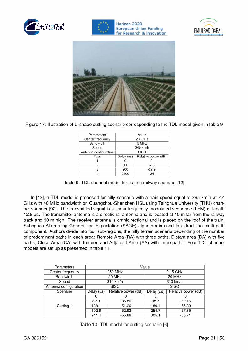
Cutting scenariosIn cutting scenario, a measurement campaign was performed on Beijing-Tianjin HSL [12] as il-

lustrated in figure 17. The authors use R&S TSMQ Radio Network Analyzer to extract the resolvablemultipath component with a maximal resolvable time delay of 20 µs. A SISO antenna configuration isused to sound the channel signal using both WCDMA signal at 2.4 GHz with 5 MHz bandwidth at 240km/h. The transmitter antenna is at 30 m away from the track on the top of the one slope wall. Thereceive antenna is on the roof of the train. The antenna characteristics are not given. The authorsprovide a four taps TDL channel model of this cutting scenario illustrated by the Table 9 with a Clas-sical/Rice Doppler spectrum distribution for the first tap and a classical Doppler spectrum distributionfor the others.

An other model for cutting is proposed in [6]. The measurements have been described previously.The environment refer to figure 16. The corresponding TDL model is given in table 10.

Hilly terrain scenariosThis environment is densely scattered with objects distributed irregularly and non uniformly. With

high altitude transmit antennas and low-altitude obstacles, the LoS component is observable and itcan be detected along the entire railway line. However, multi path components scattered/reflectedfrom the surrounding obstacles will cause serious constructive or destructive effects on the receivedsignal and therefore influence the channel’s fading characteristics [91].

GA 826152 | 53

ii

“output” — 2020/1/2 — 20:41 — page 31 — #31 ii

ii

ii

Figure 17: Illustration of U-shape cutting scenario corresponding to the TDL model given in table 9

Parameters ValueCenter frequency 2.4 GHz


Antenna configuration SISOTaps Delay (ns) Relative power (dB)

1 0 02 300 -7.33 900 -22.94 2100 -24

Table 9: TDL channel model for cutting railway scenario [12]

In [13], a TDL model is proposed for hilly scenario with a train speed equal to 295 km/h at 2.4GHz with 40 MHz bandwidth on Guangzhou-Shenzhen HSL using Tsinghua University (THU) chan-nel sounder [92]. The transmitted signal is a linear frequency modulated sequence (LFM) of length12.8 µs. The transmitter antenna is a directional antenna and is located at 10 m far from the railwaytrack and 30 m high. The receiver antenna is omnidirectional and is placed on the roof of the train.Subspace Alternating Generalized Expectation (SAGE) algorithm is used to extract the multi pathcomponent. Authors divide into four sub-regions, the hilly terrain scenario depending of the numberof predominant paths in each area: Remote Area (RA) with three paths, Distant area (DA) with fivepaths, Close Area (CA) with thirteen and Adjacent Area (AA) with three paths. Four TDL channelmodels are set up as presented in table 11.

Parameters ValueCenter frequency 950 MHz 2.15 GHz

Bandwidth 20 MHz 20 MHzSpeed 310 km/h 310 km/h

Antenna configuration SISO SISOScenario Delay (µs) Relative power (dB) Delay (µs) Relative power (dB)

Cutting 1

0 0 0 082.9 -36.86 95.7 -32.16

138.1 -51.26 180.4 -55.39192.6 -52.93 254.7 -57.35241.4 -55.66 305.1 -55.71

Table 10: TDL model for cutting scenario [6]

GA 826152 | 53

ii

“output” — 2020/1/2 — 20:41 — page 32 — #32 ii

ii

ii

Parameters ValueCenter Frequency 2.4 GHz


Antenna configuration SISOScenario Tap number Relative time delay (ns) Average path gain (dB) Doppler shift

AA

1 0 0 - fmax2 280 -8.7 fV3 640 -17.5 fV4 1350 -27.2 fV

CA

1 0 0 - fmax2 200 -11.4 fV3 450 -27.6 fV4 520 -12.7 fV5 860 -29.0 fV6 1160 -28.0 fV7 1230 -27.6 fV8 1330 -23.8 fV9 1390 -23.1 fV

10 1480 -25.9 fV11 1590 -18.7 fV12 1770 -29.1 fV13 2100 -29.7 fV

DA

1 0 0 - fmax2 230 -9.2 fmax3 1.2 -15.7 fmax4 1.6 -18.9 fmax5 2.0 -20.8 fmax

RA1 0 0 - fmax2 0.4 -15.2 fmax3 1.2 -19.7 fmax

Notes(1) fV is a random variable and fV ∼ U [- fmax,+ fmax].(2) The Doppler shift values are corresponding to the case when the train departs from the intersection point.

Table 11: TDL channel models for hilly terrain sub-regions [13]

GA 826152 | 53

ii

“output” — 2020/1/2 — 20:41 — page 33 — #33 ii

ii

ii

In [14], a measurement campaign, in hilly terrain at 2.6 GHz with 20 MHz of bandwidth alongthe Harbin-Dalian HSL at 370 km/h is studied. A 1023 bit length pseudo noise (PN) sequence mod-ulated by a BPSK generated by Agilent E4438C VSG is used. The antenna configuration is SISOone where the transmitter antenna is fixed on the operator BS. This antenna is a cross-polarizationdirectional antenna with 65°horizontal and 6.8°vertical beam width. The receiver antenna is omnidi-rectional placed on the roof of the train. The authors defined two sub-regions with different number ofpredominant paths: near region and far region and they defined for each a TDL model as illustratedon table 12.

Parameters ValueCenter frequency 2.6 GHzBandwidth 20 MHzSpeed 370 km/hAntenna configuration SISO

Scenario Delay (ns) Relative power (dB) Doppler shift*

Near region0 0 fmax

97.65 -6.77 0.5.fmax216.79 X 0.5.fmax

Far region

0 0 fmax78.12 -3.23 0.5.fmax

175.77 -7.79 0.5.fmax234.36 -11.60 0.5.fmax312.48 -16.55 0.5.fmax

Table 12: TDL channel model for near and far region of hilly terrain with fmax equal to 875 Hz [14]

In [12], a measurement campaign is performed in hilly terrain scenario on Beijing-Tianjin HSL. Thescenario is composed by a plain environment on one side and a mountain at a distance of 800 m onthe other side. The environments studied are plain, hilly terrain, U-shape cutting and station scenario.Here we focus only on the hilly terrain scenario. The authors use R&S TSMQ Radio Network Analyzerto extract the resolvable multipath component with a maximum resolvable time delay of 20 µs. A SISOantenna configuration is used to sound the channel signal using both WCDMA signal at 2.4 GHz with5 MHz bandwidth at 240 km/h. The transmitter antenna is at 30 m away from the track on the topof the one slope wall. The receive antenna is on the roof of the train. The authors provide a threetaps TDL channel model of this hilly terrain scenario illustrated by the table 13 with a Classical/RiceDoppler spectrum distribution for the first tap and a classical Doppler spectrum distribution for theothers.


Scenario Delay (µs) Relative power (dB)0 0

0.3 -7.60.6 -22

Table 13: TDL model for hilly terrain [12]

Station scenarioIn the same paper as before [12], authors defined a three taps TDL channel model for the station

scenario presented in table 14. The Doppler distribution is the same as before.

GA 826152 | 53

ii

“output” — 2020/1/2 — 20:41 — page 34 — #34 ii

ii

ii


Taps Delay (µs) Relative power (dB)1 0 02 0.3 -5.23 0.6 -8.2

Table 14: TDL model for station scenario [12]

9.3 Train to Ground Cluster Delay line channel model for high speed line scenarioThe CDL channel model represents a channel formed by several clusters of taps, which representpaths with different delays and angle of arrival. Due to the complexity to defined a CDL channelmodel, the literature is poor in term of complete CDL channel model in the railway domain. At themoment of the writing of the report, only two CDL channel model have been found for rural scenario:the WINNER II channel model D2a [7] and the IMT-A MRa channel model [10].

The Deliverables D1.1.2 V1.0 [15] and V1.2 [16] of WINNER II project related to channel modelspresent a typical open rural area scenario for high speed line. The frequency range is from 2 GHz to6 GHz with a bandwidth up to 100 MHz. The antennas (Huber+Suhner rooftop antenna SWA 0859 –360/4/0/DFRX30 - 5.25 GHz) are located on the roof of the train. The measurements were performedwith Propsound multi dimensional radio channel sounder from Elektrobit. This scenario is availablefor a speed of 350 km/h using Moving Relay Stations (MRS) on the train at 2.5 m high and with theBS at 50 m away from the track at 30 m high every 1 000-2 000 m. This scenario is presented onthe figure 18. For this WINNER II model, the total number of paths in a cluster is set at 20. While thetotal number of clusters is given by N = 8. Since the scenario is set in a rural area, the NLOS case isnot considered.

The model is expressed as CDL channel model. The parameters of LOS condition are given intable 15. In the LOS model Ricean K-factor is 7 dB. The deliverables also give all the propagationparameters for the D2a scenario.

Figure 18: D2a scenario [7]

The guidelines for evaluation of radio interface technologies for IMT-Advanced is also presentedin [10]. A model composed by a rural macro (RMa) cell scenario is referred as the typical open rural

GA 826152 | 53

ii

“output” — 2020/1/2 — 20:41 — page 35 — #35 ii

ii

ii

Parameters ValueCenter frequency 2-6 GHz

Bandwidth Up to 100 MHzSpeed 350 km/h

Antenna configuration SISO-MIMOCluster number Delay (ns) Relative Power (dB) AoD (°) AoA (°) Ray power (dB)

1 0 0.0 0.0 0.0 -0.12* -28.8**2 45 50 55 -17.8 -20.1 -21.8 12.7 -80 -27.83 60 -17.2 -13.6 86 -30.24 85 -16.15 13.4 84.4 -29.55 100 105 110 -18.1 -20.4 -22.1 -13.9 87.5 -28.16 115 -15.7 -13 -82.2 -28.77 130 -17.7 -13.9 87.5 -30.88 210 -17.3 13.7 86.2 -30.3

* power of dominant ray** Power of each other rayCluster ASD = 2°Cluster ASA = 3°Cross polarisation XPR = 12 dB

Table 15: CDL parameters channel model for D2a scenario [15] et [16]

railway scenario. The frequency range, only for this RMa scenario, is from 450 MHz to 6 GHz with abandwidth up to 100 MHz. A High Speed Line scenario is defined as B3 scenario for a train speedup to 350 km/h. This scenario covers a wide area, which can be up to 10 km. The BS antenna heightis generally in the range from 20 to 70 m. Two CDL channel models are given for the RMa channelmodel, the LOS and NLOS ones. This paper also defines all the path loss parameters for the RMascenario.

9.3.1 Conclusion

In this chapter we presented the main results found in the literature regarding radio channel modelsin HSL scenarios that can be considered to evaluate system performances (able to be implementedfor example in a radio channel emulator). The analysis conducted shows that there are a lot ofpapers dealing with a representation of some statistical channel parameters as path loss, K-factor,angle of arrival, etc. but there are not a lot of complete channel models that give a representation ofthe complex impulse response of the channel. A quite general and straightforward methodology toimplement channel model is the TDL model. We provide a review of some TDL channel model forrural, viaduct, cutting, hilly terrain and station scenarios. It is shown that, for a same scenario, differentchannel models can be defined depending of the number of representative paths for example. Another channel model that can be found in the literature is the CDL channel model which is morecomplex than TDL channel model. There are not a lot of CDL channel model in the literature due tothe complexity of model. We are able, for now, to describe only two CDL channel model. The firstone is presented in the WINNER II model created by the 3GPP. The second on is presented in theIMT-A model created by ITU. Both of them describe a CDL model for rural scenario. No more CDLchannel model has been found for other HSL scenario in the literature.

GA 826152 | 53

ii

“output” — 2020/1/2 — 20:41 — page 36 — #36 ii

ii

ii

9.4 Channel models obtained with measurements and simulations in tunnels

9.4.1 Introduction

As mentioned in the introduction of this part, most of the results in the literature present the statisticalproperties of narrow band channel characteristics such as Path Loss and K-factor and distributionsof angle of arrival or departure of the paths [68]-[87].As for the high speed line part, we decided to focus on channel models that can be used for systemevaluation, ie models that provide a description of the compex impulse response of the channel. Theliterature in this part is not studied a lot. In [88], a Saleh-Valenzuela channel model is identified withtwo main clusters. However, these papers do not give enough information about them to use it as areference channel model. In [89], the authors focused on the Kronecker and Weichselberger channelmodels. Finally, [8] provides a CDL channel model based on the WINNER procedure using a raytracing method.

In this part, we will introduce firstly, the free propagation in tunnel environment. Then, we willgive the channel models that we found in literature regarding the train to ground channel model fortunnel scenario. A CDL channel model will be also given following the WINNER approach. Finally,a TDL channel model will be defined for the train to train communications in case of inter-consistand intra-consist communications. Both of the inter-consist and intra-consist communications will beexplain in the last section.

9.4.2 Free propagation in tunnel

Radio propagation inside the tunnel is affected by several phenomena that will affect the signal prop-agation:

• wave guide effect created by the tunnel walls that act as an oversize wave guide in certainconditions as mentioned before;

• multiple reflection on the tunnel walls and diffraction on the edge that create fast variations andfading of the electromagnetic field inside the tunnel;

• an attenuation and a coupling between the inside and the outside of the tunnel that depends onthe position of the radio access point versus the tunnel axis;

• masking effects related to the presence of other trains inside the tunnel, the existence of curvesor discontinuities (enlargement - narrowing) inside the tunnel.

From a general point of view, the traditional free space radio wave propagation laws are no morevalid in tunnels. When the tunnel length can be considered as infinite without curve, if the tunnel isnot metallic and if the dimensions of the transverse section of the tunnel are large compared to thewavelength of the operating signal, the tunnel can be considered as an oversize dielectric wave guide[93]. In this case, there are different approaches and methodologies to describe radio wave prop-agation in tunnels. The objective of the different existing methodologies is to express the complexelectromagnetic field in the confined area thanks to the resolution of Maxwell equations with specificboundary conditions imposed by the characteristics of the tunnel walls.

The most used methods are: rigorous description by solving Maxwell equations [94] with mathe-matical methods (integral methods or parabolic vector equations [95], [96], [97]), asymptotic approachto solve the equations by using the optical approximation using ray tracing [98], [99], [100], [77] and

GA 826152 | 53

ii

“output” — 2020/1/2 — 20:41 — page 37 — #37 ii

ii

ii

[87] or ray launching [101]. The modal theory is also often considered and permits physical interpre-tation of some phenomenon [94]. [102] and [93] have developed the electromagnetic field equationsin the case of rectangular linear tunnel. The case of circular tunnel was treated in [103] and [104].More details can be found in [101] and [105]. This theory allows to express the electromagnetic fieldfor rectangular and circular infinite linear tunnels.

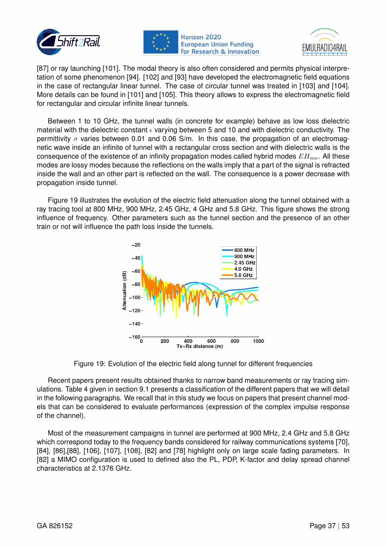
Between 1 to 10 GHz, the tunnel walls (in concrete for example) behave as low loss dielectricmaterial with the dielectric constant ε varying between 5 and 10 and with dielectric conductivity. Thepermittivity σ varies between 0.01 and 0.06 S/m. In this case, the propagation of an electromag-netic wave inside an infinite of tunnel with a rectangular cross section and with dielectric walls is theconsequence of the existence of an infinity propagation modes called hybrid modes EHmn. All thesemodes are lossy modes because the reflections on the walls imply that a part of the signal is refractedinside the wall and an other part is reflected on the wall. The consequence is a power decrease withpropagation inside tunnel.

Figure 19 illustrates the evolution of the electric field attenuation along the tunnel obtained with aray tracing tool at 800 MHz, 900 MHz, 2.45 GHz, 4 GHz and 5.8 GHz. This figure shows the stronginfluence of frequency. Other parameters such as the tunnel section and the presence of an othertrain or not will influence the path loss inside the tunnels.

Figure 19: Evolution of the electric field along tunnel for different frequencies

Recent papers present results obtained thanks to narrow band measurements or ray tracing sim-ulations. Table 4 given in section 9.1 presents a classification of the different papers that we will detailin the following paragraphs. We recall that in this study we focus on papers that present channel mod-els that can be considered to evaluate performances (expression of the complex impulse responseof the channel).

Most of the measurement campaigns in tunnel are performed at 900 MHz, 2.4 GHz and 5.8 GHzwhich correspond today to the frequency bands considered for railway communications systems [70],[84], [86],[88], [106], [107], [108], [82] and [78] highlight only on large scale fading parameters. In[82] a MIMO configuration is used to defined also the PL, PDP, K-factor and delay spread channelcharacteristics at 2.1376 GHz.

GA 826152 | 53

ii

“output” — 2020/1/2 — 20:41 — page 38 — #38 ii

ii

ii

Some general remarks for MIMO case in tunnelsIt is important to note the particularity of the case of MIMO (Multiple Input Multiple Output) sys-

tems in tunnels. [109] highlighted the decorrelation observed due to interference between the varioushybrid modes. In [110], the hypothesis of the authors is that modal diversity can be compared to spa-tial diversity for MIMO techniques. Depending on the transverse or longitudinal receiver position inthe tunnel, different modes EHmn can be excited. This hypothesis was confirmed in [111]. In [89],the authors have illustrated very clearly the influence of the hybrid modes excitation on a MIMO sys-tem performance. Using ray tracing simulations in a straight tunnel with rectangular cross section,they highlighted that when the antennas are perpendicular to the tunnel longitudinal axis, the MIMOchannel capacity is maximal. In contrary, when the antennas are parallel to the longitudinal axis, theMIMO channel capacity is minimal. These results have been also confirmed in underground minesby [112], [113], [114] and in railway tunnels by [108].

Keyholes phenomenon was highlighted by [115]. This phenomenon occurs when the distancebetween the transmitters and the receivers is large compared to the radius of the circle in which thescatters at transmission and receptions sides are situated [116]. This phenomenon exists when thesignals propagate in a corridor or a tunnel or when the transmitter ans receiver are very far to eachother in outdoor. These channels are degenerated and can be represented by a channel matrix ofrank 1 despite a total decorrelation.

The existence of a keyhole highlight the fact that a certain position in the channel, all the paths arecorrelated. In this case, the channel matrix is degenerated with only one degree of freedom (only onenon zero eigenvalue). This is very negative for MIMO performances. In [117], the authors analyzethe probability of presence of keyholes [118], [119] in various tunnel types (old and new ones). Theyshowed the big influence of tunnel dimensions and changes in the cross section dimension as wellas the fact that the tunnel is new or not. Paradoxically, the presence of keyholes does not impact thecapacity[117].

In [120] the authors analyze the influence of the variations of dimension of the tunnel transversesection on the probability of presence of keyhole. References to keyhole effects appear also in [121],[110], [122]. Generally, the higher is the correlation between the signals, the lower is the channel ca-pacity. Nevertheless, when the correlation between antennas is low, the channel matrix H presentsa low rank (equal to 1) and a keyhole phenomenon can occur. The example generally chose, is ascenario with a small hole in a wall that separates the environment between transmitter and receiver.The mathematical description of the phenomenon is given in [119].

9.4.3 Train to Ground channel model for tunnel scenario

As illustrated in table 4, only two papers give all the parameters of the models for T2G transmissions.At the moment of writing this report, we identified a Saleh-Valenzuela representation in [88] whereauthors defined two clusters but do not provide information on the various parameters to use it. Thus,we will not take it into account. The Kronecker and Weichselberger models based on correlation canalso be considered for performance evaluations as presented in [89] but it is difficult to consider themfor channel emulation. Finally, a WINNER CDL channel model is defined in [8].

WINNER CDL channel for tunnel environmentOnly one channel model based on WINNER channel model has been set up in [8] at 5.8 GHz.

The model was obtained using a Ray-Tracing tool to simulate free propagation in a given realisticdynamic scenario with two tracks and two trains. The four receiving antennas patch are fixed on theroof of the moving train. The scenario is represented figure 20. The simulated train was running at50 km/h. The authors present a 4x4 MIMO model based on 5 clusters. Each path of each cluster isdefined in terms of delay, power, AoA and AoD.

GA 826152 | 53

ii

“output” — 2020/1/2 — 20:41 — page 39 — #39 ii

ii

ii

We consider that the transformation of a CDL model into a TDL one is not straightforward, sothis reference [8] will not be considered for emulation. Therefore, the only remaining solution couldbe to generate a proper TDL model from scratch using ray-tracing simulations. This option is notconsidered for the moment.

Figure 20: Representation of the scenario simulated [8]

9.4.4 Conclusion

Today, the literature analysis conducted shows that there is no available general MIMO channel modelto describe the behavior of dynamic subway scenario in tunnel from a radio channel point of view inorder to evaluate digital communication system performances. In this section we highlighted themain results found in the literature regarding channel models in tunnels that can be considered toevaluate system performance. This topic is not yet intensively treated in the literature. A lot of papersdealing with statistical analysis of measurements in the 2-5 GHz band can provide some results onfadings and delay spread statistics. Several papers also analyze the variation of the spatial correlationdegree in the tunnel as a function of antenna polarization or antenna positions. Based on this figures,it is possible also to build simple statistical models such as Kronecker and Weichselberger models.Another channel model is a WINNER CDL channel model obtained with dynamic simulations basedon an optimized ray-tracing simulator for straight tunnels with rectangular cross section. Key holeseffect in tunnel has also been briefly presented.

GA 826152 | 53

ii

“output” — 2020/1/2 — 20:41 — page 40 — #40 ii

ii

ii

9.5 General conclusion regarding state of the art related to Channel models for Rail-way environments

The characterization of the channel models for railway environments is a large topic due to the diver-sity of common environments that a train can encounter during a ride. We have considered channelmodels obtained with measurements and simulations along high speed lines and tunnels. We iden-tified several channel models that can be used in Emulradio4rail platform for T2G communicationsalong HSL. The choice remains limited because (a) we need to have TDL, eventually CDL, modelsand (b) the number of works dealing with such models is limited. Moreover we did not find a suit-able model for the tunnel case and further measurement campaigns and data analysis are needed toderive such models.

The chosen models will prove the feasibility of a real-time evaluation of the radio link inside thecomplete platform. Extension will be necessary to improve the capabilities of the plateform: eitherdevelopping new TDL models for the missing cases or including more complex emulation solutionsthat offer higher accuracy but at the cost of complexity.

GA 826152 | 53

ii

“output” — 2020/1/2 — 20:41 — page 41 — #41 ii

ii

ii

10 Applicability analysis of the channel models for the emulation plat-form

10.1 IntroductionIn this applicability analysis we include a description of the methodology to identify the most suitablechannel models and also the summary of the proposed models to be implemented in the platform.An exhaustive survey of the state-of-the-art of radio channel models in railways has been done basedon literature study during the project and was presented in the previous section. The outcome is thatthere are different channel models in the literature but not all of them seem to be suitable to be im-plemented in channel emulator and, more specific, to provide a complete description of the channel.In particular, a description of the Doppler spectrum is missing many times.

The emulation needs to be performed under specific conditions, in order to address on an effi-cient way, the scenarios, services, perturbations and technologies that have been requested. On theother hand, there are some constraints that come from the available technology for the emulationplatform. In particular, the channel emulator only accepts tapped-delay line (TDL) channel models,therefore, all the selected channels must be TDL-based. Moreover, there is a limitation in the numberof taps that the emulator is able to handle, so we can’t accept all the TDL-based channels as they are.

10.2 MethodologyRegarding the completeness of the channel information, models should include the following infor-mation of the channel:

• Number of taps.

• Delay associated to each tap.

• Relative power associated to each tap (relative to the 1st one).

• Speed range considered.

• Doppler spectrum (i.e. distribution of the frequency shift in the Doppler domain).

• Frequency range.

• Bandwidth considered.

• Diversity (i.e. SISO, MIMO, etc.).

Consequently, the approach is to choose the TDL-based model that provides a more detaileddescription of the channel in each scenario. In case we have many of them that fulfill this condition,we will choose the one that is based on similar premises as we are (i.e. frequency bands close tothose related to LTE and IEEE 802.11, bandwidth and vehicular speed).

In particular, LTE emulation will be focused on both 900 MHz and 1.9 GHz and IEEE 802.11 (Wi-Fi) will be focused on 2.4 GHz. Therefore, in case of doubt we prefer to have channels models whosefrequencies are closer to our bands of interest.

Finally, channel models based on measurements are preferable to models based on simulationsonly.

GA 826152 | 53

ii

“output” — 2020/1/2 — 20:41 — page 42 — #42 ii

ii

ii

10.3 Summary of the channel models most suitable for emulationIn this section we summarize the channels we have found more suitable to be emulated with thepremises we have explained before. In table 16 a summary is provided.

Scenario Model CommentsHilly [123] ETSI 6 taps model at 900 MHz and 100 km/hRural [12]

Viaduct [5] Frequency band of the model (2.35 GHz) is not close to the bands of interest for this scenarioCutting [6]Tunnel [8] Provided model is a Winner model not easy to emulate

Table 16: The selected models

10.3.1 Hilly Terrain

In this scenario two models are identified.First, we consider the SISO model described in the ETSI document [123]. This model is based on

measurements in the 900 MHz band at a speed of 100 km/h. MIMO setups were not considered andinformation on Doppler spectrum is available (the classical one, which is also called Jakes’ Spectrum).The considered bandwidth is up to 5 MHz. Both the time reference and the associated power for eachtap is shown in table 17. The ETSI document present several models with 12 taps and a reducedversion with 6 taps. For each model two equivalent alternative tap settings, indicated respectively by(1) and (2) in the appropriate columns, are given. We have chosen the 6 taps model as a first proofof concept but depending on the emulator capabilities, an extension to 12 taps is feasible.

Second, another potential TDL-based model for hilly terrain can be considered [11] for SISOconfiguration. It provides the same information as [123] (including Doppler spectrum) and it is givenin table 12. It was measured at a higher speed but it is based on 2.6 GHz, which made it an interestingoption for emulation of IEEE 802.11 at 2.4 GHz. The problem is that in hilly scenarios it is very unlikelythat the train-to-ground communications will be based on IEEE 802.11 systems (which is more likelyfor urban, depots, stations and subway tunnels, but not for regional or high-speed trains).

Tap number Relative time (µs) Relative power (dB)1 (1) 0.0 (2) 0.0 (1) 0.0 (2) 0.02 0.1 0.2 -1.5 -2.03 0.3 0.4 -4.5 -4.04 0.5 0.6 -7.5 -7.05 15.0 15.0 -8.0 -6.06 17.2 17.2 -17.7 -12.0

Table 17: Selected model for Hilly terrain extracted from ETSI report in the 900 MHz band [17]

10.3.2 Rural scenario

The model is extracted from [12]. It was obtained thanks to measurements in the 2.4 GHz band inthe environment illustrated on figure 21. The TDL parameters are given in the following table 18. TheDoppler spectrum considered for each tap is the Jakes model or Classical model. The other TDLmodel that could be considered, is the GSM rural area standard model from [123] given in table givenfigure 20.

Another model is extracted from [9]. Table 19 summarizes the information.

10.3.3 Viaduct

In viaducts one TDL channel model was found in [5]. This model is based on measurements taken at2.35 GHz which is far away from the LTE bands of interest for the Emulradio4rail project. The Doppler

GA 826152 | 53

ii

“output” — 2020/1/2 — 20:41 — page 43 — #43 ii

ii

ii

Figure 21: Rural environment for HSL in China [9]

Parameter ValueCenter frequency 2.4 GHz


Antenna configuration SISOScenario Tap Delay (µs) Relative power (dB)

Rural1 0 02 0.3 -12.93 0.6 -22.9

Table 18: TDL characteristics of rural HSL model obtained in [12]

spectrum follows a discrete distribution with three possible values for the Doppler shift depending onthe region (far or not from the transmitting point) and also on the tap. In table 6 relative power andtime for each tap and Doppler shift are shown. The other parameters for this model are a bandwidthof 10 MHz, SISO-only and measurements were taken at 240 km/h.

10.3.4 Cutting

In the cutting scenario we found three different models: [6], [66], [12]. The three of them are measuredat high speeds, neither of them consider MIMO schemes and all of them provide information aboutthe Doppler spectrum. Regarding the frequency band they differ, because [6] covers both 950 MHzand 2.15 GHz; [66] covers 2.35 GHz and [12] 2.4 GHz. For this reason, we chose [6]. The TDLparameters for this model are shown in table 10 and the Doppler shift is bounded between 100and 260 Hz at 950 MHz, and 200-600 Hz at 2.15 GHz. The vehicle speed was 310 km/h and thebandwidth is 20 MHz.

10.3.5 Tunnel scenario

It is noteworthy to say that in the scientific literature there is no TDL-based model for tunnels. Thiscould be due to many different reasons, one of them the high temporal resolution that is needed tobe achieved in order to solve the multipath components that may exist on a tunnel.

Considering existing ray-tracing tool a perspective to this report could be the development ofseveral TDL models based on realistic tunnel description using simulations.

GA 826152 | 53

ii

“output” — 2020/1/2 — 20:41 — page 44 — #44 ii

ii

ii

Parameter ValueCenter frequency 1.85 GHz

Bandwidth 20 MHzSpeed 0-300 km/h

Antenna configuration SISOScenario Tap Delay (ns) Relative power (dB)

Rural1 0.2 02 1.2 -14.5

Table 19: TDL characteristics for Hilly terrain extracted from [9]

Tapnumber

Relativetime (µ s)

Relativepower (dB)

Dopplerspectrum

(1) (2) (1) (2)1 0.0 0.0 0.0 0.0 RICE2 0.1 0.2 -4.0 -2.0 CLASS3 0.2 0.4 -8.0 -10.0 CLASS4 0.3 0.6 -12.0 -20.0 CLASS5 0.4 -16.0 CLASS6 0.5 -20.0 CLASS

Table 20: GSM rural model with 6 taps in [17]

11 ConclusionsThis literature analysis performed within the Task 3.1 of WP1 in the Emulradio4rail project has per-mitted to identify a suitable TDL-based channel model for the following railway-related scenario:

• Hilly

• Rural

• Cutting

• Viaduct

. . . with the remarkable exception of tunnels.During this literature survey, we found models in some representative railway scenarios allowing

the validation of the channel emulators in the Emulradio4rail project and the first results for Experi-mental assessment of IP impairments expected for D3.2. We highlighted that the literature is incom-plete and not all railway scenarios have a model that can be used for channel emulation and radiolink performance evaluation.

This conclusion opens important perspectives and particularly the need for further works on chan-nel modelling, and especially the need for some specific measurement campaigns. Another perspec-tive is the possibility to introduce more sophisticated real-time channel emulators able to operate withgeometric channel models as well as Winner model widely considered in the standardization bodies.

GA 826152 | 53

ii

“output” — 2020/1/2 — 20:41 — page 45 — #45 ii

ii

ii

References[1] Andreas F.Molisch. Wireless communications, Second edition. Wiley, 2011.

[2] Hideichi Sasaoka. Wave Summit Course: Mobile communications. Hideichi Sasaoka ed.,2000.

[3] Fernando Perez Fontan, Veikko Hovinen, M Schonhuber, Roberto Prieto-Cerdeira, J Rivera-Castro, Pavel Valtr, J Kyrolainen, and F Teschl. Characterisation of the satellite-to-indoor prop-agation channel. pages 105 – 110, 09 2008.

[4] C. X. Wang, A. Ghazal, B. Ai, Y. Liu, and P. Fan. Channel measurements and models forhigh-speed train communication systems: A survey. IEEE Communications Surveys Tutorials,18(2):974–987, 2016.

[5] L. Liu, C. Tao, J. Qiu, H. Chen, L. Yu, W. Dong, and Y. Yuan. Position-Based Modeling forWireless Channel on High-Speed Railway under a Viaduct at 2.35 GHz. IEEE Journal onSelected Areas in Communications, 30(4):834–845, May 2012.

[6] Jianwen Ding, Lei Zhang, Jingya Yang, Bin Sun, and Jiying Huang. Broadband Wireless Chan-nel in Composite High-Speed Railway Scenario: Measurements, Simulation, and Analysis,2017.

[7] Yvo de Jong Bultitude and Terhi Rautiainen. IST-4-027756 WINNER II D1. 1.2 V1. 2 WINNERII Channel Models. EBITG, TUI, UOULU, CU/CRC, NOKIA, Tech. Rep, 2007.

[8] S. Hairoud, P. Combeau, Y. Pousset, Y. Cocheril, and M. Berbineau. WINNER model for subwaytunnel at 5.8 GHz. In 2012 12th International Conference on ITS Telecommunications, pages743–747, November 2012.

[9] Bangyan Huang, Dongping Yao, Dan Fei, Lei Xiong, and Hongfeng Qin. Development of LTE-based channel tester for high-speed scenario. In 2017 15th International Conference on ITSTelecommunications (ITST), pages 1–5, May 2017.

[10] M. Series. Guidelines for evaluation of radio interface technologies for IMT-Advanced. ReportITU, (2135-1), 2009.

[11] W. Qian, X. Chunxiu, Z. Min, and Y. Deshui. Results and analysis for a novel 2 #x00d7;2channel measurement applied in LTE-R at 2.6 GHz. In 2014 IEEE Wireless Communicationsand Networking Conference (WCNC), pages 177–181, April 2014.

[12] Liu Liu, Cheng Tao, Tao Zhou, Youping Zhao, Xuefeng Yin, and Houjin Chen. A highly efficientchannel sounding method based on cellular communications for high-speed railway scenar-ios. EURASIP Journal on Wireless Communications and Networking, 2012(1):307, December2012.

[13] Yan Zhang, Zunwen He, Wancheng Zhang, Limin Xiao, and Shidong Zhou. Measurement-Based Delay and Doppler Characterizations for High-Speed Railway Hilly Scenario, 2014.

[14] W. Qian, X. Chunxiu, W. Muqing, Z. Min, and Y. Deshui. Propagation characteristics of highspeed railway radio channel based on broadband measurements at 2.6 GHz. In 2014 IEEEWireless Communications and Networking Conference (WCNC), pages 166–170, April 2014.

[15] Ist-4-027756 winner ii d1.1.2 v1.0 - winner ii channel models part ii - radio channel measure-ment and analysis results. Technical report, 2007.

GA 826152 | 53

ii

“output” — 2020/1/2 — 20:41 — page 46 — #46 ii

ii

ii

[16] Ist-4-027756 winner ii d1.1.2 v1.2 - winner ii channel models part i - channel models. Technicalreport, 2007.

[17] Digital cellular telecommunications system (Phase 2+) (GSM) - GSM/EDGE Background forRadio Frequency (RF) requirements - 3GPP TR 45.050 version 14.0.0 Release 14. 2017.

[18] R. Torrego, M. Bouaziz, J. Soler, A. Vizzarri, M. Berbineau, and J. Moreno. Deliverable d 2.1:Solutions to emulate the radio bearer (stream b), public, h2020-s2r-oc-ip2-2018-03. 2019.

[19] J. Moreno, M. Berbineau, C. Gransart, A. Vizzari, R. Torrego, J. Soler, and Y. Yan. Deliver-able d1.1 - application layer requirements for communications systems in railway environments(stream a), public, h2020-s2r-oc-ip2-2018-03. 2019.

[20] L. Clavier, P. Mariage, S. Karbech, R. Torrego, V. Inaki, A. Arriola, V. Deniau, A. Vizarri,J. Moreno, and R. Kassi. Deliverable d1.2 - present and future railway communications sce-narios: description of perturbations with impact on railway communications (stream c), h2020-s2r-oc-ip2-2018-03, public. 2019.

[21] R. Torrego, P. Aljama, M. Berbineau, J. Soler, Y. Yan, L. Clavier, S. Kharbech, and A. Vizzarri.Deliverable d 3.1 - high-level design of radio access emulation tool (stream b), h2020-s2r-oc-ip2-2018-03, public. 2019.

[22] Jean-Marc Kwadjane. Apport de la connaissance a priori de la position de l’emetteur sur lesalgorithmes MIMO adaptatifs en environnement tunnel pour les metro. PhD thesis, PhD thesis,Universite de Lille, December 2014.

[23] Gerald Moniak. Techniques MIMO pour un lien sans fil robuste entre un bus et un poste decontrole pour une application de surveillance embarquee. PhD thesis, PhD thesis, L’Universitede Valenciennes et du Hainaut Cambresis, February 2007.

[24] A. F. Molisch. A generic model for mimo wireless propagation channels in macro- and micro-cells. IEEE Transactions on Signal Processing, 52(1):61–71, Jan 2004.

[25] J. D. Parsons. The Mobile Radio Propagation Channel. Pentech Press, 1992.

[26] J. G. Proakis. Wireless Communications. Pearso, 2007.

[27] A. Goldsmith. Digital Signal Processing, 4th Edition. Cambridge University Press, 2005.

[28] T. S. Rappaport. Wireless Communications. Prentice Hall, 2002.

[29] Ana Aguiar and James Gross. Wireless channel models. 04 2003.

[30] Michel Mfeze and Emmanuel Tonye. Comparative Approach of Doppler Spectra for FadingChannel Modelling by the Filtered White Gaussian Noise Method. International Journal ofComputer Science and Telecommunications, 6(11):1, 2015.

[31] Philip Bello. Characterization of randomly time-variant linear channels. IEEE transactions onCommunications Systems, 11(4):360–393, 1963.

[32] Gregory J. Pottie and William J. Kaiser. Principles of Embedded Networked Systems Design.Cambridge University Press, 2005.

[33] Philippe Guguen. Techniques multi-antennes emission-reception ; Applications aux reseauxdomestiques sans fil. PhD thesis, PhD thesis, INSA de Rennes, September 2003.

[34] Robert G. Gallager. Information Theory and Reliable Communication. Wiley, 1966.

GA 826152 | 53

ii

“output” — 2020/1/2 — 20:41 — page 47 — #47 ii

ii

ii

[35] C.F. Van Loan G.H. Golub. Matrix computations. Johns Hopkins university press, 1996.

[36] M. Steinbauer, A. F. Molisch, and E. Bonek. The double-directional radio channel. IEEE An-tennas and Propagation Magazine, 43(4):51–63, Aug 2001.

[37] Julien Guillet. Caracterisation et modelisation spatio-temporelles du canal de propagation ra-dioelectrique dans le contexte MIMO. PhD Thesis, INSA de Rennes, 2004.

[38] P. Bello. Characterization of randomly time-variant linear channels. IEEE Transactions onCommunications Systems, 11(4):360–393, December 1963.

[39] P. Petrus, J. H. Reed, and T. S. Rappaport. Geometrical-based statistical macrocell channelmodel for mobile environments. IEEE Transactions on Communications, 50(3):495–502, March2002.

[40] 3gpp tr 25.996 v14.0.0 (2017-03) 3rd generation partnership project technical specificationgroup radio access network spatial channel model for multiple input multiple output (mimo)simulations. Technical report, 2017.

[41] P. Almers, E. Bonek, A. Burr, N. Czink, M. Debbah, V. Degli-Esposti, H. Hofstetter, P. Kyosti,D. Laurenson, G. Matz, A. F. Molisch, C. Oestges, and H. Ozcelik. Survey of channel andradio propagation models for wireless mimo systems. EURASIP J. Wirel. Commun. Netw.,2007(1):56–56, January 2007.

[42] D. S. Baum, J. Hansen, and J. Salo. An interim channel model for beyond-3g systems: extend-ing the 3gpp spatial channel model (scm). In 2005 IEEE 61st Vehicular Technology Conference,volume 5, pages 3132–3136 Vol. 5, May 2005.

[43] wp5: Final report on link level and system level channel models. deliverable d5.4, November2005.

[44] Juha Meinila, Pekka Kyosti, Lassi Hentila, Tommi Jamsa, Essi Suikkanen, Esa Kunnari, andMilan Narandzic. Document Title: D5. 3: WINNER+ Final Channel Models.

[45] Vuokko Nurmela, Aki Karttunen, Antti Roivainen, Leszek Raschkowski, Veikko Hovinen,Juha Ylitalo EB, Nobutaka Omaki, Katsutoshi Kusume, Aki Hekkala, and Richard Weiler.Deliverable d1. 4 METIS channel models. In Proc. Mobile Wireless Commun. Enablers Inf.Soc.(METIS), page 1, 2015.

[46] Itu-r m.1225 - guidelines for evaluation of radio transmission technologies for imt-2000. Tech-nical report, 1997.

[47] M. Gudmundson. Correlation model for shadow fading in mobile radio systems. Electron. Lett.,27,23:2145–2146, 1991.

[48] A. A. M. Saleh and R. Valenzuela. A Statistical Model for Indoor Multipath Propagation. IEEEJournal on Selected Areas in Communications, 5(2):128–137, February 1987.

[49] A. Abdi and M. Kaveh. A space-time correlation model for multielement antenna systems inmobile fading channels. IEEE Journal on Selected Areas in Communications, 20(3):550–560,April 2002.

[50] Q. H. Spencer, B. D. Jeffs, M. A. Jensen, and A. L. Swindlehurst. Modeling the statistical timeand angle of arrival characteristics of an indoor multipath channel. IEEE Journal on SelectedAreas in Communications, 18(3):347–360, March 2000.

GA 826152 | 53

ii

“output” — 2020/1/2 — 20:41 — page 48 — #48 ii

ii

ii

[51] Ke Guan, Zhangdui Zhong, and Bo Ai. Assessment of LTE-R Using High Speed RailwayChannel Model. pages 461–464. IEEE, April 2011.

[52] L. Tian, X. Yin, Q. Zuo, J. Zhou, Z. Zhong, and S. X. Lu. Channel modeling based on randompropagation graphs for high speed railway scenarios. In 2012 IEEE 23rd International Sym-posium on Personal, Indoor and Mobile Radio Communications - (PIMRC), pages 1746–1750,September 2012.

[53] T. Zhou, C. Tao, S. Salous, L. Liu, and Z. Tan. Channel sounding for high-speed railwaycommunication systems. IEEE Communications Magazine, 53(10):70–77, October 2015.

[54] T. Zhou, C. Tao, S. Salous, L. Liu, and Z. Tan. Implementation of an LTE-Based Channel Mea-surement Method for High-Speed Railway Scenarios. IEEE Transactions on Instrumentationand Measurement, 65(1):25–36, January 2016.

[55] Tomas Domınguez-Bolano, Jose Rodrıguez-Pineiro, Jose A. Garcıa-Naya, and Luis Castedo.Experimental Characterization of LTE Wireless Links in High-Speed Trains. Wireless Commu-nications and Mobile Computing, 2017:1–20, 2017.

[56] Jingya Yang, Bo Ai, Danping He, Longhe Wang, Zhangdui Zhong, and Andrej Hrovat. A Sim-plified Multipath Component Modeling Approach for High-Speed Train Channel Based on RayTracing, 2017.

[57] A. Ghazal, Y. Yuan, C. X. Wang, Y. Zhang, Q. Yao, H. Zhou, and W. Duan. A Non-StationaryIMT-Advanced MIMO Channel Model for High-Mobility Wireless Communication Systems.IEEE Transactions on Wireless Communications, 16(4):2057–2068, April 2017.

[58] J. Bian, J. Sun, C. X. Wang, R. Feng, J. Huang, Y. Yang, and M. Zhang. A WINNER #x002b;Based 3-D Non-Stationary Wideband MIMO Channel Model. IEEE Transactions on WirelessCommunications, 17(3):1755–1767, March 2018.

[59] R. He, Z. Zhong, B. Ai, G. Wang, J. Ding, and A. F. Molisch. Measurements and Analysisof Propagation Channels in High-Speed Railway Viaducts. IEEE Transactions on WirelessCommunications, 12(2):794–805, February 2013.

[60] K. Guan, Z. Zhong, B. Ai, and T. Kurner. Deterministic Propagation Modeling for the RealisticHigh-Speed Railway Environment. In 2013 IEEE 77th Vehicular Technology Conference (VTCSpring), pages 1–5, June 2013.

[61] Rongchen Sun, Cheng Tao, Liu Liu, Zhenhui Tan, Lingwen Zhang, and Tao Zhou. NonisotropicScattering Characteristic in an Alternant Tree-Blocked Viaduct Scenario on High-Speed Rail-way at 2.35 GHz, 2014.

[62] D. He, J. Yang, K. Guan, B. Ai, Z. Zhong, Z. Zhao, D. Miao, and H. Guan. Ray-tracing simulationand analysis of propagation for 3gpp high speed scenarios. In 2017 11th European Conferenceon Antennas and Propagation (EUCAP), pages 2890–2894, March 2017.

[63] T. Zhou, C. Tao, S. Salous, and L. Liu. Measurements and Analysis of Angular Characteristicsand Spatial Correlation for High-Speed Railway Channels. IEEE Transactions on IntelligentTransportation Systems, 19(2):357–367, February 2018.

[64] R. He, Z. Zhong, B. Ai, J. Ding, Y. Yang, and A. F. Molisch. Short-Term Fading Behavior inHigh-Speed Railway Cutting Scenario: Measurements, Analysis, and Statistical Models. IEEETransactions on Antennas and Propagation, 61(4):2209–2222, April 2013.

GA 826152 | 53

ii

“output” — 2020/1/2 — 20:41 — page 49 — #49 ii

ii

ii

[65] L. Tian, J. Zhang, and C. Pan. Small Scale Fading Characteristics of Wideband Radio Chan-nel in the U-Shape Cutting of High-Speed Railway. In 2013 IEEE 78th Vehicular TechnologyConference (VTC Fall), pages 1–6, September 2013.

[66] R. Sun, C. Tao, L. Liu, and Z. Tan. Channel Measurement and Characterization for HSR U-Shape Groove Scenarios at 2.35 GHz. In 2013 IEEE 78th Vehicular Technology Conference(VTC Fall), pages 1–5, September 2013.

[67] K. Guan, Z. Zhong, B. Ai, and T. Kurner. Propagation Measurements and Analysis for TrainStations of High-Speed Railway at 930 MHz. IEEE Transactions on Vehicular Technology,63(8):3499–3516, October 2014.

[68] Y. Zhang, Y. Liu, J. Sun, C. X. Wang, and X. Ge. Impact of Different Parameters on ChannelCharacteristics in a High-Speed Train Ray Tracing Tunnel Channel Model. In 2017 IEEE 85thVehicular Technology Conference (VTC Spring), pages 1–5, June 2017.

[69] K. Guan, B. Ai, Z. Zhong, C. F. Lopez, L. Zhang, C. Briso-Rodrıguez, A. Hrovat, B. Zhang,R. He, and T. Tang. Measurements and Analysis of Large-Scale Fading Characteristics inCurved Subway Tunnels at 920 MHz, 2400 MHz, and 5705 MHz. IEEE Transactions on Intelli-gent Transportation Systems, 16(5):2393–2405, October 2015.

[70] J. Li, Y. Zhao, J. Zhang, R. Jiang, C. Tao, and Z. Tan. Radio channel measurements andanalysis at 2.4/5ghz in subway tunnels. China Communications, 12(1):36–45, January 2015.

[71] C. Gentile, F. Valoit, and N. Moayeri. A raytracing model for wireless propagation in tunnelswith varying cross section. In 2012 IEEE Global Communications Conference (GLOBECOM),pages 5027–5032, December 2012.

[72] K. Guan, Z. Zhong, B. Ai, R. He, B. Chen, Y. Li, and C. Briso-Rodrıguez. Complete PropagationModel in Tunnels. IEEE Antennas and Wireless Propagation Letters, 12:741–744, 2013.

[73] L. Zhang, C. Briso, J. R. O. Fernandez, J. I. Alonso, C. Rodrıguez, J. M. Garcıa-Loygorri, andK. Guan. Delay Spread and Electromagnetic Reverberation in Subway Tunnels and Stations.IEEE Antennas and Wireless Propagation Letters, 15:585–588, 2016.

[74] Concepcion Garcia-Pardo, Jose-Maria Molina-Garcıa-Pardo, Martine Lienard, Davy P. Gaillot,and Pierre Degauque. Double directional channel measurements in an arched tunnel andinterpretation using ray tracing in a rectangular tunnel. Progress In Electromagnetics Research,22:91–107, 2012.

[75] K. Guan, Z. Zhong, J. I. Alonso, and C. Briso-Rodriguez. Measurement of Distributed AntennaSystems at 2.4 GHz in a Realistic Subway Tunnel Environment. IEEE Transactions on VehicularTechnology, 61(2):834–837, February 2012.

[76] K. Guan, Z. Zhong, B. Ai, and C. Briso-Rodriguez. Propagation mechanism modelling in thenear region of circular tunnels. Antennas Propagation IET Microwaves, 6(3):355–360, February2012.

[77] K. Guan, X. Lin, D. He, B. Ai, Z. Zhong, Z. Zhao, D. Miao, H. Guan, and T. Kurner. Scenariomodules and ray-tracing simulations of millimeter wave and terahertz channels for smart railmobility. In 2017 11th European Conference on Antennas and Propagation (EUCAP), pages113–117, March 2017.

[78] X. Ye, X. Cai, H. Wang, and X. Yin. Tunnel and Non-Tunnel Channel Characterization forHigh-Speed-Train Scenarios in LTE-A Networks. In 2016 IEEE 83rd Vehicular TechnologyConference (VTC Spring), pages 1–5, May 2016.

GA 826152 | 53

ii

“output” — 2020/1/2 — 20:41 — page 50 — #50 ii

ii

ii

[79] H. d Zheng and X. y Nie. GBSB Model for MIMO Channel and Its Space-Time CorrelataionAnalysis in Tunnel. In 2009 International Conference on Networks Security, Wireless Commu-nications and Trusted Computing, volume 1, pages 8–11, April 2009.

[80] Y. Jia, M. Zhao, W. Zhou, and D. Peng. Measurement and statistical analysis of 1.89ghzradio propagation in a realistic mountain tunnel. In 2015 International Conference on WirelessCommunications Signal Processing (WCSP), pages 1–5, October 2015.

[81] D. J. Cichon, T. C. Becker, and W. Wiesbeck. Determination of time-variant radio links inhigh-speed train tunnels by ray optical modeling. In IEEE Antennas and Propagation SocietyInternational Symposium. 1995 Digest, volume 1, pages 508–511 vol.1, June 1995.

[82] X. Cai, X. Yin, X. Cheng, and A. Perez Yuste. An Empirical Random-Cluster Model for SubwayChannels Based on Passive Measurements in UMTS. IEEE Transactions on Communications,64(8):3563–3575, August 2016.

[83] Xiao Chen, Yuntian Pan, Yiming Wu, and Guoxin Zheng. Research on Doppler spread ofmultipath channel in subway tunnel. In 2014 IEEE International Conference on CommunictionProblem-solving, pages 56–59, December 2014.

[84] C. Briso-Rodriguez, J. M. Cruz, and J. I. Alonso. Measurements and Modeling of Dis-tributed Antenna Systems in Railway Tunnels. IEEE Transactions on Vehicular Technology,56(5):2870–2879, September 2007.

[85] E. Masson, Y. Cocheril, M. Berbineau, J. P. Ghys, J. Kyrolainen, and V. Hovinen. 4 #x00d7;4MIMO channel sounding in tunnels for train-to-wayside communications. In 2012 InternationalConference on Wireless Communications in Underground and Confined Areas, pages 1–5,August 2012.

[86] L. Zhang, J. R. Fernandez, C. B. Rodrıguez, C. Rodrıguez, J. Moreno, and K. Guan. Broadbandradio communications in subway stations and tunnels. In 2015 9th European Conference onAntennas and Propagation (EuCAP), pages 1–5, May 2015.

[87] Danping He, Bo Ai, Ke Guan, Zhangdui Zhong, Bing Hui, Junhyeong Kim, Heesang Chung,and Ilgyu Kim. Stochastic Channel Modeling for Railway Tunnel Scenarios at 25 GHz. ETRIJournal, 40(1):39–50, February 2018.

[88] R. He, Z. Zhong, B. Ai, K. Guan, B. Chen, J. I. Aionso, and C. Briso. Propagation channel mea-surements and analysis at 2.4 GHz in subway tunnels. Antennas Propagation IET Microwaves,7(11):934–941, August 2013.

[89] Yann Cocheril, Marion Berbineau, Pierre Combeau, and Yannis Pousset. On the Importance ofthe MIMO Channel Correlation in Underground Railway Tunnels. Journal of Communication,4(4):224–231, May 2009.

[90] ”sencity rail antenna: 1399.17.0039 huber+suhner data sheet,” huber+suhner ag rf industrial.Technical report, 2010.

[91] Yu Liu, Ammar Ghazal, Cheng-Xiang Wang, Xiaohu Ge, Yang Yang, and Yapei Zhang. Channelmeasurements and models for high-speed train wireless communication systems in tunnelscenarios: a survey. Science China Information Sciences, 60(10):101301, October 2017.

[92] Yan Zhang, Ove Edfors, Peter Hammarberg, Tommy Hult, Xiang Chen, Shidong Zhou, LiminXiao, and Jing Wang. A general coupling-based model framework for wideband mimo chan-nels. IEEE Transactions on Antennas and Propagation, 60(2):574–586, 2012.

GA 826152 | 53

ii

“output” — 2020/1/2 — 20:41 — page 51 — #51 ii

ii

ii

[93] A. G. Emslie and R. L. Lagace. Theory of the Propagation of UHF Radio Waves in Coal MineTunnels. IEEE-ANT, 23(2):192–205, March 1975.

[94] Jorge Avella Castiblanco. Electromagnetic modeling for antenna design and specificationsin tunnels of arbitrary cross-section and answering to the electromagnetic constraints of theenvironment of the railway domain. Lille 1, April 2013.

[95] H. Chang, Y. Wu, S. Lu, W. Cheng, and M. Sheng. Field analysis of dielectric waveguide de-vices based on coupled transverse-mode integral equation-numerical investigation. ProgressIn Electromagnetics Research, 97:159–176, 2009.

[96] SY. Reutskiy. The methods of external excitation for analysis of arbitrarily-shaped hollow con-ducting waveguides. Progress In Electromagnetics Research, 82:203–226, 2008.

[97] A. V. Popov and Ning Yan Zhu. Modeling radio wave propagation in tunnels with a vectorialparabolic equation. IEEE-ANT, 48(9):1403–1412, Sep 2000.

[98] S. F. Mahmoud. Characteristics of Electromagnetic Guided Waves for Communication in CoalMine Tunnels. IEEE-COM, 22:1547–1554, October 1974.

[99] M. Agunaou, S. Belattar, P. Mariage, and P. Degauque. Propagation d’ondeselectromagnetiques hyperfrequences a l’interieur d’un metro - Modelisation numerique del’influence des changements de section. Revue Transports et Securite, 64:55–68, 1998.

[100] K. Guan, B. Ai, R. He, Z. Zhong, T. Xu, C. Briso-Rodriguez, and A. Hrovat. Stochastic Mod-eling for Extra Propagation Loss of Tunnel Curve. In 2016 IEEE 83rd Vehicular TechnologyConference (VTC Spring), pages 1–5, May 2016.

[101] E. Masson. etude de la propagation des ondes electromagnetiques dans les tunnels courbesde section non droite pour des applications metro et ferroviaire. PhD thesis, Universite dePoitiers, Decembre 2010.

[102] K. D. Laakman and W. H. Steier. Waveguides: characteristic modes of hollow rectangulardielectric waveguides. Applied Optics, 15(5):1334–1340, May 1976.

[103] D. G. Dudley and S. F. Mahmoud. Linear source in a circular tunnel. IEEE Transactions onAntennas and Propagation, 54(7):2034–2047, July 2006.

[104] D. G. Dudley, S. F. Mahmoud, M. Lienard, and P. Degauque. On wireless communication intunnels. In 2007 IEEE Antennas and Propagation Society International Symposium, pages3305–3308, June 2007.

[105] Jorge Avella Castiblanco. Electromagnetic Modeling for Antenna design and Specifications intunnels of any shape answering to the electromagnetic constraints of the environment of therailway domain. PhD thesis, University of Lille, April 2013.

[106] M. Lienard, P. Degauque, J. Baudet, and D. Degardin. Investigation on MIMO channels insubway tunnels. IEEE Journal on Selected Areas in Communications, 21(3):332–339, April2003.

[107] J. M. Molina-Garcia-Pardo, M. Lienard, A. Nasr, and P. Degauque. Wideband analysis of largescale and small scale fading in tunnels. In 2008 8th International Conference on ITS Telecom-munications, pages 270–273, October 2008.

GA 826152 | 53

ii

“output” — 2020/1/2 — 20:41 — page 52 — #52 ii

ii

ii

[108] E. Masson, Y. Cocheril, M. Berbineau, J.P. Ghys, V. Hovinen, and A. Roivanen. Mimo channelcharacterization in subway tunnel for train-to-wayside applications. IEEE ITST Proceedings- In-ternational Conference in Intelligent Transportation Systems-Telecommunications, Taipei, Tai-wan, pages 732–736, November 2012.

[109] M. Lienard, P. Degauque, J. Baudet, and D. Degardin. Investigation on MIMO channels insubway tunnels. IEEE-SAC, 21(3):332–339, Apr 2003.

[110] J. M. Molina-Garcia-Pardo, M. Lienard, P. Degauque, C. Garcia-Pardo, and L. Juan-Llacer.Mimo channel capacity with polarization diversity in arched tunnels. IEEE Antennas and Wire-less Propagation Letters, 8:1186–1189, 2009.

[111] J. A. Castiblanco, D. Seetharamdoo, M. Berbineau, M. Ney, and F. Gallee. Determination ofantenna specification and positioning for efficient railway communication in tunnels of arbitrarycross section. In ITS Telecommunications (ITST), 2011 11th International Conference on,pages 678–683, Aug 2011.

[112] A. E. Forooshani, R. D. White, and D. G. Michelson. Effect of antenna array properties onmultiple-input-multiple-output system performance in an underground mine. IET Microwaves,Antennas Propagation, 7(13):1035–1044, October 2013.

[113] A. E. Forooshani, A. A. Lotfi-Neyestanak, and D. G. Michelson. Optimization of antenna place-ment in distributed MIMO systems for underground mines. IEEE-WCOM, 13(9):4685–4692,Sept 2014.

[114] A. E. Forooshani, C. Y. T. Lee, and D. G. Michelson. Effect of antenna configuration on MIMO-based access points in a short tunnel with infrastructure. IEEE-COM, 64(5):1942–1951, May2016.

[115] David Gesbert, Helmut Bolcskei, Dhananjay Gore, and Arogyaswami Paulraj. Mimo wirelesschannels: Capacity and performance prediction. In Global Telecommunications Conference,2000. GLOBECOM’00. IEEE, volume 2, pages 1083–1088. IEEE, 2000.

[116] David Gesbert and Jabran Akhtar. Breaking the barriers of shannon’s capacity: An overview ofmimo wireless systems. Signal Processing, 1(B2):B3, 2002.

[117] J. Moreno, L. de Haro, C. Rodrıguez, L. Cuellar, and J. M. Riera. Keyhole estimation of anMIMO-OFDM train-to-wayside communication system on subway tunnels. IEEE Antennas andWireless Propagation Letters, 14:88–91, 2015.

[118] D. Chizhik, G. J. Foschini, M. J. Gans, and R. A. Valenzuela. Keyholes, correlations, andcapacities of multielement transmit and receive antennas. IEEE-WCOM, 1(2):361–368, Apr2002.

[119] P. Almers, F. Tufvesson, and A. F. Molisch. Keyhole effect in MIMO wireless channels: Mea-surements and theory. IEEE-WCOM, 5(12):3596–3604, December 2006.

[120] D. G. Dudley, M. Lienard, S. F. Mahmoud, and P. Degauque. Wireless propagation in tunnels.IEEE-APM, 49(2):11–26, April 2007.

[121] Javier Alonso Valdesueiro, Benjamin Izquierdo, and Jordi Romeu. On 2x2 mimo observablecapacity in subway tunnels at-band: An experimental approach. Antennas and Wireless Prop-agation Letters, IEEE, 9:1099–1102, 2010.

GA 826152 | 53

ii

“output” — 2020/1/2 — 20:41 — page 53 — #53 ii

ii

ii

[122] Concepcion Sanchis-Borras, Jose-Maria Molina-Garcia-Pardo, Martine Lienard, and Pierre De-gauque. Performance evaluation of mimo-ofdm in tunnels. Antennas and Wireless PropagationLetters, IEEE, 11:301–304, 2012.

[123] Etsi 145 005 v13.3.0, digital cellular telecommunications system (phase 2+) (gsm) gsm/edgeradio transmission and reception, (3gpp ts 45.0145 005 v13.3.0, release 13). 2017.

GA 826152 | 53

deliverable d 1.3 characterization of the railway

Documents