deliverable 6 - brunel university london

- 1 -

Deliverable 6.1

Authors T. Owens, C. Zhang, T.Itagaki

(Brunel), Jan Outters (IRT), J

Lauterjung (R&S), M. Martucci

(PUSP), D. Bouquet, B. Mazieres, J.

Prudent (TDF), P. Christ, Ingo

Gaspard, Stefan Ritscher, Gerd

Zimmermann, P. Christ (T-Systems)

Title Radio spectrum, traffic engineering

and resource management

Last update 27 April 2006

Version 1.5

Circulation PUBLIC

- 2 -

Contents Glossary .........................................................................................................................5

Chapter 1 Introduction ...................................................................................................6

The overall conclusions are presented in Chapter 9.Chapter 2 Frequency Planning.....7

Chapter 2 Frequency Planning.......................................................................................8

2.1 Background ..........................................................................................................8

2.1.1 Aim of this chapter........................................................................................8

2.1.2 Objectives of this chapter..............................................................................8

2.2 Frequencies used for television channels.............................................................8

2.2.1 Frequency usage in the United Kingdom......................................................9

2.2.2 Frequency usage in Germany......................................................................18

2.2.3 Frequency usage in France..........................................................................22

2.2.4 Frequency usage in The Netherlands [3] ....................................................25

2.2.5 Frequency usage in Brazil...........................................................................26

2.2.6 Summary.....................................................................................................27

2.3 Frequency planning after introducing DVB-T/H...............................................28

2.3.1 Frequency planning in the simulcast stage .................................................28

2.3.2 Frequency planning in the switchover stage...............................................28

2.3.3 Summary.....................................................................................................29

2.4 Network topologies for DVB-T/H.....................................................................29

2.4.1 Dedicated DVB-T and DVB-H network.....................................................30

2.4.2 DVB-T/H co-cited with a cellular Telco network ......................................31

2.4.3 Existing DVB-T network and DVB-H sharing MUX ................................32

2.5 Protection ratio and Single Frequency Networks ..............................................33

2.5.1 Protection ratio............................................................................................33

2.5.2 Single Frequency Networks........................................................................33

2.6 Conclusions........................................................................................................34

2.7 References..........................................................................................................34

Chapter 3 Densification and rules for “cellularized” DVB-T/H planning...................36

3.1 Introduction........................................................................................................37

3.2 Cell range ...........................................................................................................37

3.2.1 Field strength propagation curves...............................................................37

3.2.2 Coverage range prediction ..........................................................................40

3.3 Coverage planning .............................................................................................47

3.3.1 Single frequency networks (SFN)...............................................................47

3.3.2 Multi frequency networks (MFN)...............................................................54

3.3.3 Sectorized cell layout..................................................................................60

3.3.4 Antenna down-tilting ..................................................................................62

3.3.5 Illumination of MFN cells by SFNs............................................................64

3.4 References..........................................................................................................68

Chapter 4 SFN Network Benefits for DVB-H Networks ............................................69

4.1 Elementary analysis ...........................................................................................69

4.1.1 Assumptions................................................................................................69

4.1.2 Derivation of the optimal distance..............................................................70

4.2 Simulation based analysis ..................................................................................72

4.2.1 Assumptions................................................................................................72

4.2.2 Results.........................................................................................................73

4.2.3 Analysis.......................................................................................................76

4.3 Case of Metz city ...............................................................................................76

4.3.1 Site configurations: Scy-Chazelles ; Metz-C2R ; Metz- St-Julien .............76

- 3 -

4.3.2 Required Field strength...............................................................................77

4.3.3 Results.........................................................................................................78

4.4 Conclusions........................................................................................................79

Chapter 5 Study of SFN for DVB-H networks............................................................80

5.1 Assumptions.......................................................................................................80

5.1.1 DVB specifications .....................................................................................80

5.1.2 Transmission ...............................................................................................80

5.1.3 Reception ....................................................................................................80

5.1.4 Field strength ..............................................................................................81

5.1.5 Configurations.............................................................................................82

5.2 Prediction coverages ..........................................................................................83

5.2.1 Site configurations ......................................................................................83

5.2.2 Simulation parameters ................................................................................83

5.2.3 Configuration 1: HTx = 150 m, ERP = 5 kW, 3 sites.................................84

5.2.4 Configuration 2: HTx = 75 m, ERP = 400 W, 10 sites ................................85

5.2.5 Configuration 3: HTx = 50 m, ERP = 100 W, 15 sites ................................86

5.3 Synthesis ............................................................................................................88

5.3.1 Covered areas..............................................................................................88

5.4 Conclusions........................................................................................................88

Chapter 6 DVB-H, GSM900, GSM1800 and UMTS cositing analysis ......................89

6.1 Introduction........................................................................................................89

6.1.1 Frequency bands of studied systems...........................................................89

6.1.2 Decoupling between antennas.....................................................................89

6.1.3 Spurious emissions......................................................................................90

6.1.4 Inter-modulation products...........................................................................90

6.1.5 Sensitivity degradation................................................................................90

6.1.6 Blocking......................................................................................................92

6.2 Required isolation between systems ..................................................................93

6.3 DVB-H and radiocom services cositing architectures .......................................99

6.3.1 General points .............................................................................................99

6.3.2 DVB-H and GSM900 ...............................................................................100

6.3.3 DVB-H and GSM1800 .............................................................................103

6.3.4 DVB-H and UMTS...................................................................................107

6.4 References........................................................................................................110

Chapter 7 Coverage Planning and Dimensioning in DVB-T/H ................................111

7.1 Introduction......................................................................................................111

7.1.1 Aim of this chapter....................................................................................111

7.1.2 Objectives of this chapter..........................................................................111

7.2 Parameter definition in coverage planning for DVB-T/H ...............................111

7.2.1 Coverage degree definition .......................................................................111

7.2.2 Network parameters and ranges used in the simulations ..........................113

7.3 SFN inner self-interference and outer-interference .........................................114

7.3.1 Inner self-interference in a SFN................................................................114

7.3.2 Outer interference in a SFN ..........................................................................115

7.4 Coverage planning simulation .........................................................................117

7.4.1. Field strength prediction ..........................................................................118

7.4.2 Outage probability computation ...............................................................119

7.4.3 The number of pixels and pixel resolution used in the simulations..........121

7.4.4 Comparison of the sum methods of lognormal distribution variables......125

7.4.5 Simulation procedure ....................................................................................127

- 4 -

7.5 Cell dimensioning and optimal cell radius.......................................................128

7.5.1 Procedure to compute the optimal cell size ..............................................128

7.5.2 The optimal cell radius for different network topologies .............................132

7.6. SFN gain .........................................................................................................135

7.6.1 SFN gain without frequency reuse................................................................135

7.6.2 SFN gain with a frequency reuse: .............................................................138

7.6.3 The combination of the use of the optimal cell radius figure and the SFN

gain figure ..........................................................................................................139

7.7 Conclusions......................................................................................................140

7.8 References:.......................................................................................................141

Chapter 8 DVB-T/-H receiver performance ..............................................................143

8.1 Test set-up........................................................................................................143

8.2 Transmission mode ..........................................................................................144

8.3 Test results .......................................................................................................144

Chapter 9 Conclusions ...............................................................................................147

A1. Frequency allocation in Germany [26] ...........................................................150

A2. Frequency allocation in France [26]: ..............................................................156

A3: k-LNM method from [1].................................................................................161

A4. Simulation Model Validation..........................................................................162

A5. Site Configurations .........................................................................................163

A6. The optimal radius for one single cell.............................................................164

A7. The SFN optimal cell radius with the guard interval=1/32 and without

frequency reuse ......................................................................................................166

A8. The SFN optimal cell radius with the guard interval=1/4 and without frequency

reuse .......................................................................................................................169

A9. SFN gain with the guard interval=1/32 without frequency reuse ...................172

A10. The SFN gain with the guard interval=1/4 without frequency reuse............175

A11. The optimal cell radius for SFN size = 3 with a Reuse factor, guard interval =

1/4 ..........................................................................................................................178

A12. The SFN gain for SFN size = 3 with reuse factor, guard interval=1/4; ........183

A13. The optimal cell radius of SFN size = 7 with a reuse factor, guard interval =

1/4 ..........................................................................................................................187

A14. The SFN gain for SFN size = 7 with a reuse factor, guard interval=1/4 ......192

- 5 -

Glossary

ANFR Agence Nationale des Fréquences

CSA Conseil Supérieur de l’Audiovisuel

CEPT European Conference of Postal and Telecommunications

Administrations

DECT Digital Enhanced Cordless Telecommunications

DTT Digital Terrestrial Television

DVB-T Digital Video Broadcasting - Terrestrial

DVB-H Digital Video Broadcasting -Handheld

E-GSM Enhanced GSM

GSM Global System for Mobile Communications

IMT-2000 International Mobile Telecommunications 2000

PAL Phase Alternation Line

PMR Private Mobile Radio

PAMR Public Access Mobile Radio

SAB Services Ancillary to Broadcasting

TACS Total Access Communications System

UHF Ultra High Frequency

UMTS Universal Mobile Telecommunications System (3G mobile standard)

VCR Video Cassette Recorder

VHF Very High Frequency

- 6 -

Chapter 1 Introduction

One of the core objectives of Work Package 6 is to study and define new network

planning rules (frequency allocation, cell size, cell bit rates) that will support the

deployment of denser and localized broadcast networks.

Deliverable D6.1 defines by means of simulations and measurements network

engineering rules that will enable an efficient use of broadcast spectrum. They will

contribute to the definition of protection ratio and frequency allocation management.

Chapter 2 identifies frequencies available for DVB-T/H broadcast in several European

countries and in Brazil. It does this by stating the current frequency planning with

respect to the simulcast stage of analogue and digital TV in the transition to digital

TV in these countries and by presenting the possible network topologies for DVB-T/H

broadcast and highlighting the consequences for frequency planning of each of these

topologies.

In chapter 3 the cell ranges for different DVB-T/-H reception modes are given for

different transmitter heights / powers and for rural as well as for urban environments.

For different single frequency network (SFN) structures coverage probability

predictions are done and analysed. For multi-frequency networks (MFN)

characterized mainly by their frequency reuse or cluster size different approaches are

analysed.

In mobile telecommunication networks sectorizing of cells is applied to increase

capacity without additional base station locations and down-tilting the antennas of the

radio network’s transmitters is heavily used, especially in small cells, to effectively

lower the cell range in areas were high capacity is demanded and to have a sharp

transition at the cell border with the neighbouring cells. To investigate network

topologies for DVB-H MFNs that are similar to mobile telecommunication network

topologies sectorization of hexagonal cells into 6 x 60° sectors and 3 x 120° sectors

and antenna down-tilting are considered.

Combining the benefits of SFNs with the cellular layout of MFNs to distribute more

localized content leads to the idea of illuminating the hexagonal cell area by an SFN

whose transmitters are located in the corners of the hexagon. The case where 3

transmitters with 120° sector antennas in every second corner of the hexagonal cell

are used to illuminate the cell is considered as a means of lowering the cluster size

thus lowering the number of frequencies required to deliver full area coverage.

Chapter 4 presents a theoretical evaluation of the gain in network coverage due to a

SFN network to appraise the added coverage area compared to an MFN network.

Chapter 5 attempts to determine, at a broadcast operator investment cost level, what is

the best configuration for a DVB-H SFN network deployment. Results of simulations

made with the TDF proprietary radio planning tool for several configurations, that due

to a TDF proprietary cost function based on CAPEX are known to lead to similar

investment costs, with working assumptions close to future deployments, are

presented.

Chapter 6 presents cositing issues between the DVB-H system and mobile

telecommunication services (GSM900, GSM1800, and UMTS). The main topic is

Electro-Magnetic Compatibility (EMC) between radio systems.

- 7 -

Chapter 7 presents a basic approach to modelling DVB-T/H network coverage

planning and investigates the dimensioning criteria in a wide area SFN network.

In Chapter 8 to validate the performance of the RF front-end incorporated in the

DVM400 test probe developed in WP6 Task 3, and to verify some of the conclusions

for network planning, a number of tests are reported that were carried out in

accordance with the test methodology described in the DVB-H Validation Task Force

final report [ETSI TR 102 401 v1.1.1 (2005-06)].

The overall conclusions are presented in Chapter 9.

- 8 -

Chapter 2 Frequency Planning

2.1 Background

2.1.1 Aim of this chapter

• To identify frequencies available for DVB-T/H broadcast in several European

countries.

2.1.2 Objectives of this chapter

• To state the current spectrum usage in some of EU countries, namely the

United Kingdom, Germany, France and The Netherlands, of analogue and

digital TV. To state as an example of the current spectrum usage of analogue

and digital TV in an emerging economy the current spectrum usage of

analogue and digital TV in Brazil.

• To state the current frequency planning with respect to the simulcast stage of

analogue and digital TV in the transition to digital TV.

• To present the possible network topologies for DVB-T/H broadcast and

highlight the consequences for frequency planning of each of these topologies.

Following disappointing growth in 2001 and 2002, the European DVB-T market

exhibited large subscriber growth in 2003. During 2003 the DVB-T market grew in

the United Kingdom, Sweden, Finland, Italy, Netherlands and Germany. At the end of

2003, there were 3.9 Million DVB-T households viewing DVB-T services in Europe

of which about 3 Million are viewers of Freeview services in the United Kingdom.

Berlin-Brandenburg is the only region in Europe where analogue TV has been

switched off. In some German cities like Berlin, Cologne, Düsseldorf, Bonn, Munich,

Hannover, Hamburg, the analogue signal is already partially switched off and will

completely be switched off in the near future.

Because the progress of the rollout of digital TV in the countries of Europe is

different, this chapter focuses on the frequency usage in three countries with large

home markets, the United Kingdom, Germany and France, together with The

Netherlands as its approach to digital roll-out has some particularly distinctive

features. The progress of the rollout of digital TV in Brazil is considered as an

example of digital roll out in an emerging economy. For the countries considered, this

chapter highlights the frequency usage of terrestrial analogue TV, the penetration of

terrestrial digital TV, and the arrangements for the transition to the terrestrial

analogue TV switch-off.

2.2 Frequencies used for television channels

Frequencies used for analogue TV are mainly in the bands III, IV and V. Therefore, to

identify the spectrum used by analogue TV in the countries considered, the frequency

allocation schemes in bands III to V will be examined first.

- 9 -

2.2.1 Frequency usage in the United Kingdom

2.2.1.1 Spectrum allocation

In the United Kingdom the channels used by analogue broadcasters, and thus subject

to release when the digital switchover is complete, are the 46 frequency channels 21

to 68, with the exception of channels 36 and 38; Channel 36 is used for radar and

VCRs, and Channel 38 is used for radio astronomy. The existing digital services are

interleaved between the analogue services. Therefore, there is 368 MHz to be re-

planned for the continuation of digital television and for other possible uses. There is

no band III television in UK. Figure 2.1 gives a more clear view of the television

channel distribution in UK

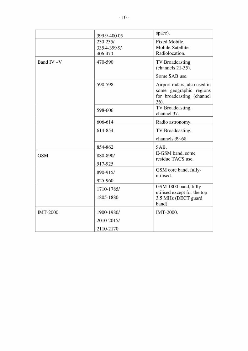
Table 2.1 shows the frequency usage in the UK above band III (condensed from [14]

and [15]).

Table 2.1 Frequency usage in UK above band III.

BAND Sub-band (MHz) Current UK use

174-217.5 Mobile (PMR and PAMR) Band III

217.5-230 Broadcasting and Mobile

services on a no

interference to

Broadcasting basis.

230⋅0-328⋅6 Fixed Mobile.

Radiolocation.

Radio Astronomy.

Mobile-Satellite.

328⋅6-335⋅4 Aeronautical-Radio-

Navigation.

399⋅9-400⋅05 Radio Navigation-Satellite.

400.05-400.15 Standard frequency and

time signal satellite (400.1

MHZ)

400.15-401 Meteorological-satellite.

Space research. Mobile-

Satellite. Meteorological

aids. Space Operations.

401-406 Meteorological aids.

Space Operation.

Fixed Mobile except:

Aeronautical.

Meteorological-Satellite

(Earth to space).

406-406.1/ Mobile-Satellite (Earth to

- 10 -

399⋅9-400⋅05 space).

230-235/

335⋅4-399⋅9/

406-470

Fixed Mobile.

Mobile-Satellite.

Radiolocation.

470-590 TV Broadcasting

(channels 21-35).

Some SAB use.

590-598 Airport radars, also used in

some geographic regions

for broadcasting (channel

36).

598-606 TV Broadcasting,

channel 37.

606-614 Radio astronomy.

614-854 TV Broadcasting,

channels 39-68.

Band IV –V

854-862 SAB.

880-890/

917-925

E-GSM band, some

residue TACS use.

890-915/

925-960

GSM core band, fully-

utilised.

GSM

1710-1785/

1805-1880

GSM 1800 band, fully

utilised except for the top

3.5 MHz (DECT guard

band).

IMT-2000 1900-1980/

2010-2015/

2110-2170

IMT-2000.

- 11 -

200

150

100

50

21 34 39 68

num

ber o

f analo

gue T

V tran

smissio

ns in

UK

0

UHF t el evi si on channel

Figure 2.1: Distribution of UK television transmission in Band IV/V [23]

The total number of television transmissions in the UK is about 6350 analogue and

DTT (from the 1100+ transmitting stations, plus 350 self-help schemes believed to be

on-air). On average, each channel is re-used 138 times throughout the UK [23]

2.2.1.2 Present analogue television coverage

The broadcasters provide 4/5 national network analogue television services to a

regulated minimum level of service based on using an outdoor receiving aerial at

rooftop height (10 metres).

In practice, nearly all UK households can receive the four national network analogue

services and around 80% a fifth national service.

The white areas in Figure 2.2 indicate the areas in the UK where there is no service.

These areas are sparsely populated. Frequency channels are reused as indicated by the

colour scheme in Figure 2.2.

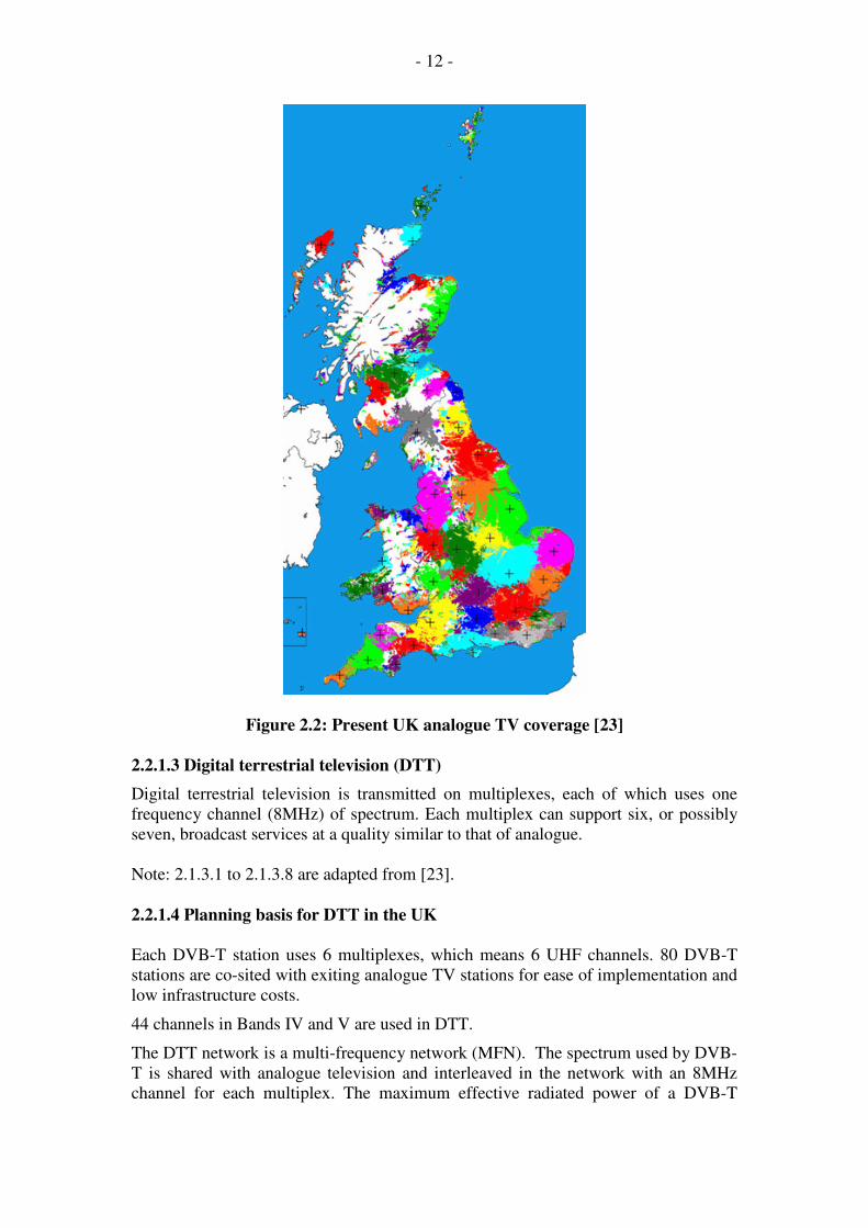
- 12 -

Figure 2.2: Present UK analogue TV coverage [23]

2.2.1.3 Digital terrestrial television (DTT)

Digital terrestrial television is transmitted on multiplexes, each of which uses one

frequency channel (8MHz) of spectrum. Each multiplex can support six, or possibly

seven, broadcast services at a quality similar to that of analogue.

Note: 2.1.3.1 to 2.1.3.8 are adapted from [23].

2.2.1.4 Planning basis for DTT in the UK

Each DVB-T station uses 6 multiplexes, which means 6 UHF channels. 80 DVB-T

stations are co-sited with exiting analogue TV stations for ease of implementation and

low infrastructure costs.

44 channels in Bands IV and V are used in DTT.

The DTT network is a multi-frequency network (MFN). The spectrum used by DVB-

T is shared with analogue television and interleaved in the network with an 8MHz

channel for each multiplex. The maximum effective radiated power of a DVB-T

- 13 -

transmitter is about 20dB below that of an analogue transmitter. The planned covered

area assumes fixed reception but will provide some portable reception as well.

Table 2.2 below shows the UK DTT multiplex licensees and their mode of operation.

(72% of households are able to receive all 6 multiplexes, assuming ideal receiving

aerials.)

Table 2.2 UK DTT Situation [16] [23]

Multiplex

Licence

1 2 A B

(Freeview)

C

(Freeview)

D

(Freeview)

Operator BBC D3&4

(ITV+C4)

SDN

(C5+S4C+ntl)

BBC Crown

Castle

Crown

Castle

DVB-T

Mode

16QAM 64QAM 64QAM 16QAM 16QAM 16QAM

Coverage 87% 81% 79% 85% 81% 72%

2.2.1.5 The DTT transmitter network

DTT was launched in 1998 with 80 transmitting stations on-air. There have since been

many small changes to the network to improve coverage.

Figure 2.3 DTT transmitters in UK [23]

2.2.1.6 DTT Multiplex coverage equalisation

- 14 -

The initial network plan provided Mux BBC to 81% of UK households but Mux D,

which was ITV Digital, to only 64% of UK households. The ‘core’ coverage was only

56%, that is, where all 6 multiplexes could be received. Following the launch of DTT

in the UK it became clear that the ‘core’ coverage effected the take up of DTT. Work

proceeded to equalise the coverage, by increasing the transmitter powers where

possible. [Figure 2.4]

Figure 2.4: UK DTT Multiplex coverage equalisation [23]

2.2.1.7 Network choices (SFN/MFN)

It is recognised that SFNs can offer improved spectrum efficiency with a typical

saving of 1/3 but they require a free VHF/UHF channel over the whole of the target

service area. SFNs also can give greater uniformity of coverage for portable reception,

but a relatively dense network of lower-power transmitters is required.

In the UK there were no free channels for regional SFNs. The prime requirement was

for fixed rooftop reception. MFNs allowed DTT transmissions to be interleaved with

analogue channels making use of adjacent channels to analogue from most TV

stations.

2.2.1.8 DVB-T channel interleaved planning

The planning is based on the planning scenario 1 in the TG 6/8 report [24].

- 15 -

“The primary assumption made for this scenario is that all existing or planned

analogue assignments1 would need to be protected by every new digital requirement

for the indefinite future. However, the analogue assignments will continue in use

without any changes and their coverage areas will be effected only to a certain extent

by new digital requirements.” [24]

“DVB-T can make use of channels adjacent to analogue transmission at a given

station. Considering the fact that adjacent channel analogue/analogue transmissions

interfere with each other, adjacent analogue/DVB-T transmissions can be co-sited

because DVB-T is lower power (won’t interfere with analogue) and it is more rugged

(analogue won’t interfere with DVB-T). Adjacent channels are extensively used in the

UK plan.

Nevertheless, not all DVB-T channels can be located adjacent to the analogue service,

other channels had to be found to provide 6 multiplexes at some stations and these

channels may give different coverage resulting in unequal coverage between

multiplexes.

It is not possible to achieve universal DTT coverage whilst the analogue network

remains in service” [23]

2.2.1.9 Channels used at a single transmitting station

“Most of the channels are used in groups of 4 for the 4 national analogue services

(BBC One, BBC Two, ITV 1 and ‘Channel 4’). The ‘Five’ service was planned

separately (and much later) and is accommodated mainly in Channel 35 and Channel

37. Each analogue service or DTT multiplex requires one frequency channel so some

transmitting stations radiate 11 different television transmissions (others fewer, and

some even more than 11).” [23]

Figure 2.5: Off-Air Signals at BBC R&D [23]

D1-D6 (the square wave) represents the 6 digital channels, the spikes reprents the

anologue TV signals.

- 16 -

2.2.1.10 Co-ordination of DTT after Chester 97

“The UK had rules on which to base our negotiations with European neighbours.

Other countries started planning DVB-T services – the UK could now make bilateral

agreements on a station for station basis. Nevertheless, Chester 97 rules are too strict

to allow the UK and its neighbours achieve their required coverage.

Relaxations have been agreed bilaterally and detailed planning methods adopted to

achieve the desired objectives including terrain based predictions and complicated

antenna designs” [23]

Figure 2.6: Co-ordination of UK DVB-T with neighbouring countries

2.2.1.11 ITU Regional Radiocommunications Conference, May/June 2006

RRC-06 scope

1. Digital broadcasting planning in the bands:

174-230 MHz (Band III)

470-862 MHz (Band IV and V, Channels 21 to 69)

2. Sound and television broadcasting

3. Other radio services having international status

4. RRC-06 impact upon UK:

• T-DAB in Band III (current use and planned future use)

• Mobile radio services in Band III

Negotiations

required

Correspondence

only

No co-ordination is

required with the

remaining countries

BELBELBELBELBELBELBELBELBEL

ALBALBALBALBALBALBALBALBALB

ANDANDANDANDANDANDANDANDAND

AUTAUTAUTAUTAUTAUTAUTAUTAUT

BIHBIHBIHBIHBIHBIHBIHBIHBIHBULBULBULBULBULBULBULBULBUL

HRVHRVHRVHRVHRVHRVHRVHRVHRV

CYPCYPCYPCYPCYPCYPCYPCYPCYP

CZECZECZECZECZECZECZECZECZE

DNKDNKDNKDNKDNKDNKDNKDNKDNK

ESTESTESTESTESTESTESTESTEST

FINFINFINFINFINFINFINFINFIN

MKDMKDMKDMKDMKDMKDMKDMKDMKD

FFFFFFFFF

DDDDDDDDD

GRCGRCGRCGRCGRCGRCGRCGRCGRC

HNGHNGHNGHNGHNGHNGHNGHNGHNG

ISLISLISLISLISLISLISLISLISL

IRLIRLIRLIRLIRLIRLIRLIRLIRL

IIIIIIIII

LVALVALVALVALVALVALVALVALVA

LIELIELIELIELIELIELIELIELIE

LTULTULTULTULTULTULTULTULTU

LUXLUXLUXLUXLUXLUXLUXLUXLUX

MLTMLTMLTMLTMLTMLTMLTMLTMLT

MDAMDAMDAMDAMDAMDAMDAMDAMDA

MCOMCOMCOMCOMCOMCOMCOMCOMCO

HOLHOLHOLHOLHOLHOLHOLHOLHOL

NORNORNORNORNORNORNORNORNOR

POLPOLPOLPOLPOLPOLPOLPOLPOL

PORPORPORPORPORPORPORPORPOR

ROUROUROUROUROUROUROUROUROU

RUSRUSRUSRUSRUSRUSRUSRUSRUS

SMRSMRSMRSMRSMRSMRSMRSMRSMR

SVKSVKSVKSVKSVKSVKSVKSVKSVK

SVNSVNSVNSVNSVNSVNSVNSVNSVN

EEEEEEEEE

SSSSSSSSS

SUISUISUISUISUISUISUISUISUI

TURTURTURTURTURTURTURTURTUR

UKRUKRUKRUKRUKRUKRUKRUKRUKR

GGGGGGGGG

CVACVACVACVACVACVACVACVACVA

- 17 -

• DVB-T in Bands IV and V

• Aeronautical radars in Ch 36

• Radio astronomy in Ch 38

• Spectrum designated for release following digital switchover (the “digital

dividend”)

• Programme-making servies in Bands III, IV and V , including Ch 69;

2.2.1.12 Spectrum trading and liberalisation in UK

“Spectrum trading and liberalisation has been introduced in bands traditionally used

for telecommunications. However, the distinction between broadcasting and

communications is becoming less clear as services continue to converge and some

broadcasting services are likely to appear in non-traditional bands in the future.

Mobile media is an important concept in that a handheld terminal can combine

broadcast reception with 3G connectivity and services. As is typical in such initiatives,

there is international standardisation activity. Some proposals for spectrum envisage

fitting DVB-H within a DVB-T framework but a standalone channel is an alternative.

The flexible spectrum regime which the UK is trying to create opens up the possibility

of acquiring a channel for mobile media. However, if it is to be combined with 3G to

make converged services, then for international roaming it would help if there was

some international spectrum harmonisation.

Changing spectrum use is a very slow process and the shortcomings in assigned

spectrum are overcome by expensive engineering methods and innovative

technologies. Using more appropriate spectrum could have as great an impact as a

major technology step.

Ofcom is changing from Command and Control to Market Mechanisms plus some

Licence-Exempt use. The Market Mechanisms are that the regulator partitions

spectrum and ownership and use are driven by market forces.”[29]

Allocation and Management Methods

1. “On –demand” assignment

2. Band plans/ harmonisation

3. “Beauty contests”

4. Administered Incentive Pricing

• Regulator can over-recover costs

• Price based on value compared with alternatives

• Price should influence usage

5. Auctions

• Fairest method of assignment.

• Auction design difficult (or may distort outcome)

• New/Existing operator difference

• UK 3G auction excessive payments

• Normal allocation method for new spectrum in future

6. Spectrum trading

• Based on economic ideas (market mechanisms)

- 18 -

• Permits changes in ownership and use

• Started in December 2004 in UK

• Transfers of licences

• Liberalisation of use of permitted

• Ofcom forecasts 72% of spectrum allocated by trading approach by

2010

“Spectrum trading and liberalisation has been introduced in bands traditionally used

for telecommunications and gives greater flexibility. The distinction between

broadcasting and communications is becoming less clear. Services continue to

converge and some services are likely to appear in non-traditional bands in

future.”[29]

2.2.1.13 The UK Government’s ‘vision’ for a digital future

The Government has not specified explicitly what it expects to be in place before

analogue television can be switched off, but it expects:

digital coverage (of one form or another) to match the present coverage of

public service analogue television

affordable digital receiving equipment ‘accessible’ to 95% of consumers

switch over to occur between 2006 and 2010

penetration (at least 70% of the UK population)

The Government has issued a ‘Digital Television Action Plan’ which has mandated

the setting up of a spectrum planning group to produce plans that would allow ‘DTT

only use of the spectrum’ (bands IV and V).

The Government acknowledges that switch over will be a sequence in time with

geographical phasing.

The likely end result will be a mix of different platforms, although the terrestrial

platform will be a principal concern because most viewers still rely on it. [23]

2.2.2 Frequency usage in Germany

2.2.2.1 Currently used spectrum

From [3]:

“In Germany bands I, III and IV/V are currently being used for the transmission of

analogue terrestrial television. In band I these are channels 2 to 4 and in band III

channels 5 to 11 each with a bandwidth of 7 MHz. This corresponds to a bandwidth of

70 MHz. Channel 12 was assigned to digital sound broadcasting T-DAB in the

Wiesbaden Plan 1995 and is no longer used by television in Germany. In Band IV/V

channels 21 to 60 are used for analogue television. In total, 50 channels are currently

being used by analogue terrestrial television in Germany.”

Figure 2.7 gives a general view of the frequency allocation for analogue and digital

TV in channels 05 to 65 in Berlin. Table A1 lists the detailed frequency allocation in

the VHF-UHF band in Germany.

- 19 -

Figure 2.7: Channel Usage in Berlin [25]

2.2.2.2 Future spectrum needs after the analogue switch-off

From [3]:

“Due to the digitalisation of television transmission broadcasters will no longer need

band I and can make channels 2 to 4 - corresponding to 21 MHz - available to the

spectrum management authorities for other purposes. Also, two further channels in

band III are intended to be used additionally to Plan WI 95 for T-DAB. Therefore, in

the VHF-band around 35 MHz (5 channels) will no longer be used in future for

terrestrial television and can be released for other services.

To facilitate the transition from analogue to digital broadcasting, channels 64 to 66 are

available for DVB-T. Unlike in some other European countries, channels 61 to 63 and

67 to 69 will not be available for broadcasting in Germany in the medium term

although they could become available in the long-term. Moreover, radio astronomy

services must be protected in channel 38 and its use for broadcasting is highly

restricted or not possible. Within the VHF- and UHF- bands 49 channels are available

in total for DVB-T.

Spectrum needs for DVB-T depend primarily on the number of programmes and

envisaged service goals and hence on the expansion of DVB-T networks. In Germany

requirements for DVB-T are expected for 24 to 30 programmes or 6 multiplexes with

the aim of portable indoor or outdoor reception, i.e. without rooftop aerials. This is to

improve the acceptance of terrestrial television, which has been strongly diminished

over the past few years due to the relatively small number of programmes available.

Mobile reception also serves this purpose and hence is part of the strategic

considerations for DVB-T. To achieve this envisaged goal, a preferably robust

transmission mode has to be selected. A compromise must be found between

transmittable data capacity and susceptibility to interference. Hence, Germany has

opted for the DVB-T variant 16QAM with code rate 2/3. Higher-level modulation

such as 64QAM (code rate 7/8) can enable almost twice the data rate but is very

- 20 -

sensitive to interference and therefore is at best suitable for reception via rooftop

aerials. With the chosen 16QAM (R=2/3) variant one can accommodate 4 PAL

quality TV programmes in an 8 MHz TV channel. Given that one needs around 7 TV

channels for full area coverage in Europe, this means 6-7 multiplexes. With the

selected DVB-T variant one could realise the envisaged 24 to 28 programmes. This

would approximate the number of analogue programmes that are transmitted by cable

today and ought to suffice for an improved acceptance of terrestrial television.”

Most of the German “Länder” have now published their digital TV rollout plans. The

experience of the successful introduction of DVB-T in Berlin will be used in most

“Länder” as the model with a short simulcast phase. In Berlin digital TV was offered

with sufficient transmission power for the private and public broadcasters in

November 2002. After less than 6 months analogue TV from private broadcasters was

switched off. The released spectrum was used for another multiplex and to improve

the coverage and reliability of digital services. For the wider Berlin area the SFN

topology was used which required 2-3 transmitter sites for each frequency. In August

2003 the analogue transmission of the public broadcast services ended. The released

spectrum was used to further improve the coverage and to pilot data services (DVB-

H/T). By the end of 2003, more digital receivers had been sold in Berlin than there

had been households depending on analogue terrestrial TV in 2001. This success was

mainly due to the availability of cheap receivers (e.g. 69 Euro), the very good

coverage of DVB-T (portable indoor and mobile reception) right from the beginning,

and the coordination of all major players (public and private broadcasters, network

operators, manufacturers) together with the Landesmedienanstalt (media board) of

Berlin.

The transition to digital TV will be finalised for the major 15 urban areas of Germany

by 2006. The last analogue TV transmitter should be switched off 2010. By 2010

there should be stationary reception for 95% of the population. Nevertheless, the final

coverage of DVB-T will depend on the market success of DVB-T and there are no

concrete rollout plans for Germany as a whole.

2.2.2.3 Digital terrestrial television

Figure 2.8 and Table 2.3 show the current reception area of DTT in Germany.

An example of Channel allocation in the Frankfurt area is given in Figure 2.9. One

channel (Ch 8) is in the VHF band, the others are all in the UHF band. Ch 8 and Ch

22 carry 3 programmes plus a MHP data service each. The other channels carry 4

programmes. Ch 64 will be operational in spring 2005. Here, 1 programme is replaced

by a media service.

- 21 -

Table 2.3: Overview of the areas in Germany where DVB-T signals can be

received

Area Start of DVB-T

switch-over

Date of

switch-off

of analogue

services

Number of

multiplexes

1. DVB-T in normal operation (analogue services switched off)

2. DVB-T operation started in 2004

3. DVB-T operation to start in 2005 4. DVB-T operation not before 2006

Figure 2.8: DVB-T reception areas: current situation in Germany Status of

November 2004

- 22 -

Figure 2.9: Channel allocation in the Frankfurt

2.2.3 Frequency usage in France

The CSA has opted for a mixed national digital network, basically, a bit of both

models: MFN on the one hand and SFN on the other hand.

The planning of the frequencies is carried out within the UHF band used in parallel to

analogue transmissions (channels 21 to 65), with the objective of minimising the

frequency re-planning of gap-fillers necessary to ensure the continuity of service of

the analogue reception. Frequency planning is made with the priority of using the

main sites currently used to broadcast analogue television

Frequency reassignment:

An operational structure in charge of the realisation on a large scale of the analogue

frequency re-channelling has been created by the CSA. This structure, called “GIE

fréquences”, is using the ANFR re-farming fund. The re-channelling operations for

230 frequencies have already been made.

- "GIE Fréquences" represents analogue channels. It is negotiating with the

French agency in charge of frequencies, ANFR, on the one hand and

monitoring the contractors.

- There are 3 contractors: TDF handles the transmission side- Espace

Numérique won the tender to handle Communication and reception. A third

player is to handle the call centre.

- TDF has already reassigned over 260 frequencies between 2003 & 2004 to

GIE.

- 23 -

The CSA believes that 1500 reassignments for the 105 designated areas will be

necessary. For the first two DTT phases, about 400 reassignments will have to be

made between now and September 2005.

The objective for terrestrial digital television is to reach coverage of 35 % of the

French population by the 31st of March 2005 (17 sites).

Note:

The planning of the first sites is published with some details on the CSA server.

Planning of the remaining sites is on going progressively.

French DTT pre-launch coverage (free-to-air programmes)

DTT Channels

From the 31st of March 2005, 14 free-to-air channels will be broadcast:

TF1, France 2, France 3, France 4, France 5, Canal + (non-encrypted broadcast), M6,

Arte, Direct 8, W9, TMC, NT1, NRJ 12, La Chaîne parlementaire

The agreed composition of the multiplexes should be:

M1: France 2, France 3, France 4, France 5, Arte, and La Chaîne Parlementaire

M2: EUROPE 2 TV, Canal J*, Direct 8, TMC, BFM, Gulliver

- 24 -

M3: Canal +*, I télé, Sport+, CANAL+ Cinéma*, and Planète*

M4: W9, M6 music, TF6*, Paris Première*, NT1, and AB1*

M5: To be dedicated to DVB-H

M6: TF1, LCI(*), Eurosport*, TPS Star*, and NRJ 12

* Pay-TV, will start in September 2005

The composition of the multiplex can be subject to changes. A ministerial co-

ordination group is established and is now meeting regularly with the participation of

all the key players. Furthermore, an association for the promotion of DTT in France

has been created.

The CSA finalised in June 2003, jointly with the selected applicants, the agreement

between the CSA and each DTT service editor. Since, the editors holding user rights

for the same radio resource jointly proposed a multiplex operator. The multiplex

operators have been created by the DTT licence holders, sharing the same multiplex,

and have received their authorizations for frequency usage.

Distributors who wish to market authorized service editors' programmes to the public

will have to make a declaration to the CSA.

Service editors, authorised to operate television services, and requiring payment from

users, must make the appropriate agreements, ensuring that each reception terminal

receives all the programmes and all services relating to it. These agreements should be

made within two months of the issuance of receipt of the declarations made by the

commercial distributors. Service editors holding an authorisation will have to ensure

that programmes begin on the date and in the conditions laid down in their

authorisation. This date will be set by the CSA in consideration of the development

and investment plans forecast, and allowing for the time needed to solve any pending

issues.

The CSA will also collaborate in the implementation by the public authorities of

measures enabling a smooth transition from analogue to digital television and to

ensure the viable development of DTT.

The time schedule for starting the digital transmissions was set by the CSA.

The CSA has decided to dedicate the 5th multiplex to DVB-H.

It has now been decided to operate the free to air programmes in MPEG-2 and the

pay-TV programmes in MPEG-4/H-264. Hence the launch of pay TV may be delayed.

2.2.3.1 Future spectrum usage

The objectives for terrestrial digital television are to reach coverage of 50 % in

September 2005 (32 sites), and in the long term, of 80 % to 85 % of the French

population (105 sites). By The end of June 2005 500,000 receivers were sold.

From September 05, launch of commercial pay per view DTT (in a 6 month window)

with the following channels:

AB1, Canal + (encrypted), Eurosport, LCI, Paris-Première, TF6,TPS Star

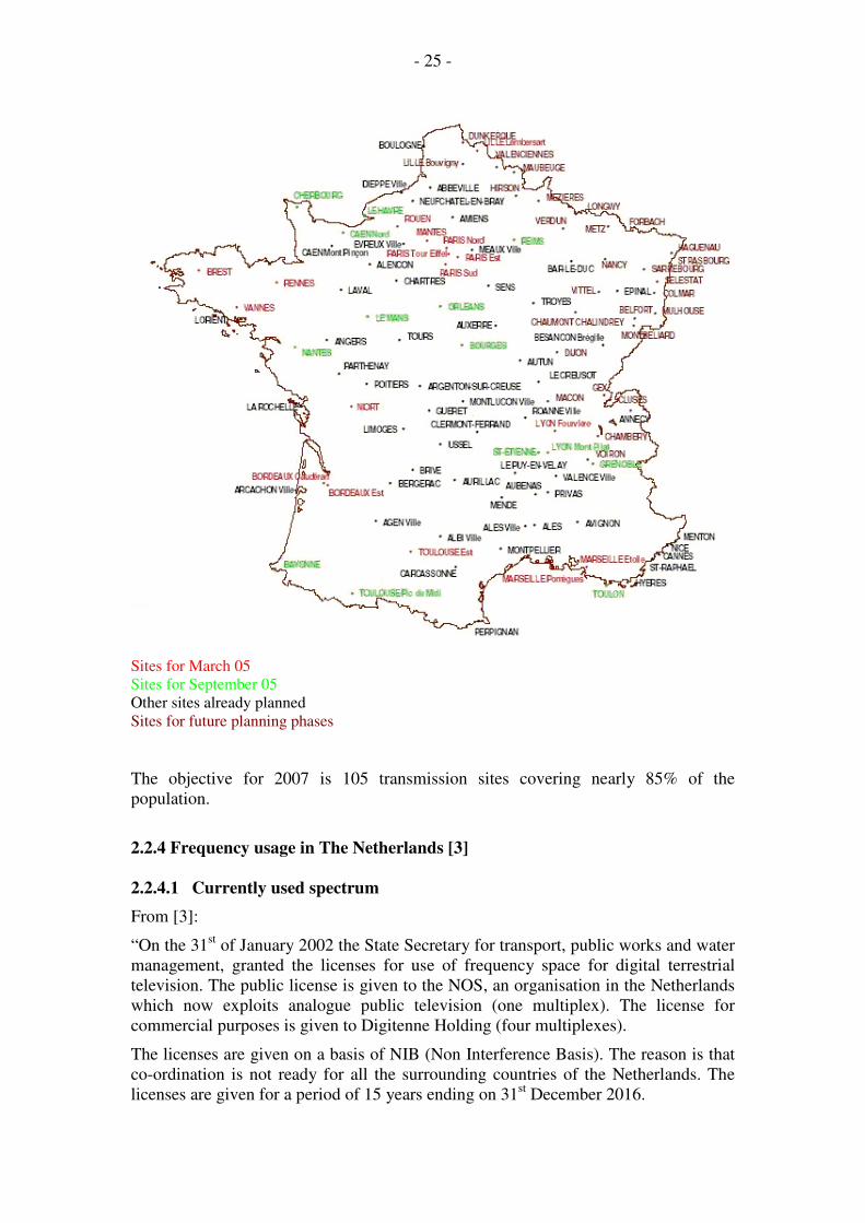
- 25 -

Sites for March 05

Sites for September 05

Other sites already planned

Sites for future planning phases

The objective for 2007 is 105 transmission sites covering nearly 85% of the

population.

2.2.4 Frequency usage in The Netherlands [3]

2.2.4.1 Currently used spectrum

From [3]:

“On the 31st of January 2002 the State Secretary for transport, public works and water

management, granted the licenses for use of frequency space for digital terrestrial

television. The public license is given to the NOS, an organisation in the Netherlands

which now exploits analogue public television (one multiplex). The license for

commercial purposes is given to Digitenne Holding (four multiplexes).

The licenses are given on a basis of NIB (Non Interference Basis). The reason is that

co-ordination is not ready for all the surrounding countries of the Netherlands. The

licenses are given for a period of 15 years ending on 31st December 2016.

- 26 -

Digitenne and NOS started together in April 2003 with regular digital commercial

transmissions in part of the so-called Randstad area and they are now in a position to

finalise their multiplexes in the complete Randstad area.”

2.2.4.2 Digital Switch-over

From [3]:

“A government appointed advisory commission proposed that a switch off should be

realised around 2007, provided that some necessary conditions are fulfilled at that

time.

Public broadcasters are now studying in detail how the transition to digital could take

place in the fastest way. There is a proposal using the regional frequencies with the

following schematic steps:

1) Simulcast the regional program in DVB-T on a temporary frequency.

2) After half a year analogue broadcasting will be switched off, and the

frequency will then be used to transmit all 3 nationwide programs plus the

regional program in DVB-T.

3) Step 2 is the beginning of the half-year simulcast for the 3 nationwide

programs in that region.

Even this scheme would take a period of some 3-4 years to complete the switch over.

2.2.4.3 Cable interference

From [3]:

“The license holder, the cable operator and the Government will cover problems that

can be solved by using good cable material. The Government will contribute an

amount of 2.7 million Euros to solving such problems. The cost of solving problems

that cannot be solved by using good cable material must be paid for by the license

holder.”

2.2.5 Frequency usage in Brazil

2.2.5.1 Current spectrum allocation

From [21]:

Sub-band (in MHZ) Use in Brazil

54-72 Broadcasting of audio and video –

transmission and retransmission of VHF

signal.

72-76 Restrict radiation – radio command systems

and listening aid devices

76-87.8 Broadcasting – basic channel distribution on

VHF and UHF transmission.

87.8-88 Neighbourhood broadcasting.

- 27 -

88-108 Audio Broadcasting – basic channel

distribution on FM transmission.

108-144 Aeronautical – radio – navigation space to

Earth.

Meteorological-satellite. Space research.

Mobile-Satellite. Meteorological aids.

174-216 Broadcasting – basic channel distribution on

VHF and UHF transmission and

retransmission.


VHF and UHF retransmission.

608-614 Radio – astronomy.


VHF and UHF transmission and

retransmission.

2.2.5.2 Plan of digital spectrum usage

From [22]:

“Channel planning

Channels:

1. Transition phase: “Simulcasting” of analogue and digital television in the

UHF (preferentially) and the VHF high (channels 7 to 13) bands.

2. Digital phase: Digital TV only”

Digital TV is planned to be allocated channels 14 to 59 only considering the

possibility of frequency re-utilisation. And, if the system hasn’t full capacity of reuse,

the channels between 60 and 69 could be used also. The basic plan foresees 1893

digital channels over all Brazilian states (From [22]).

2.2.6 Summary

In the UK if all the frequencies used by analogue TV are released for use by Digital

TV, then 368MHz will become available for use by Digital TV. During the simulcast

period, the frequencies available for Digital TV are more limited. However, as long as

the interference to the existing services is below a certain level, a frequency can be

used for Digital TV.

In Germany 50 channels are currently used for analogue TV (counting in channel 12).

During the simulcast stage, additional channels 64 and 66 will be available for digital

broadcasting. Therefore, within the VHF- and UHF- bands 49 channels will be

available for DVB-T after the switch over.

In France 45 (21-65) channels are used for analogue TV and an additional UHF

frequency band will be planned for DVB-T during the simulcast period.

The situation in The Netherlands in terms of the channel allocation is still under

review as is the planned data for the switch over.

The UK, Germany and France have all planned switch over for 2010. However, Italy

and Finland are planning switch over as early as 2006 and Belgium, Denmark,

Portugal plan to switch over in 2007. Sweden has planned to switch over in 2008.

- 28 -

Brazil plans to use UHF and VHF bands in the transition phase. The digital TV is

planned to be allocated channels 14 to 59. Channels 60-69 will also be used if the

system hasn’t full capacity of reuse.

2.3 Frequency planning after introducing DVB-T/H

2.3.1 Frequency planning in the simulcast stage

In the simulcast phase, to enable a soft transition from analogue to digital TV (in

Germany there will be a short simulcast phase of less than one year. The transition

will be complete for all major urban areas in Germany by 2006), as a rule, this phase

will entail increased spectrum needs. If the frequency used for analogue TV is not

changed, then additional channels must be assigned to transmit the digital TV signal.

(Otherwise, DVB-T/H must use the same frequency with the exiting services as long

as they do not interfere with each other.)

If spectrum will be available during this phase for DVB-H it is to be expected that

there will be less available than when this phase is complete. This probably means

that if DVB-H is to be delivered during this phase, its frequencies may need to be

reassigned after this phase.

A major issue is that countries are not going through simulcast stage in phase. As each

country comes out of simulcast and tries to re-assign frequencies this will have an

impact on its neighbours. 2.3.2 Frequency planning in the switchover stage

The EU’s Radio Spectrum Policy Group (RSPG) adopted an opinion in November

2004 on “The Spectrum Implications of Switchover to Digital Broadcasting”[27]

This recognised:

• The benefits of switchover- more efficient and flexible spectrum use, the

spectrum dividend, and the contribution to the strategic goals of the “Lisbon

Agenda”

• The importance of coordination between member states on spectrum

management to assist a quick and efficient switchover

• The benefits of a common approach to the transition period

• The need for initiatives to promote consumer benefits

• The value of flexibility in planning for both broadcasting and other radio

services, with a technology-neutral approach for the latter

Digital Dividend

When the analogue TV services have been closed down, there will be some spectrum

that can be used for other purposes, such as for:

1. More digital TV services to roof-top antennas

2. Digital TV services to mobile/handheld devices

3. Digital HDTV

4. DAB services( in band III)

5. Non-broadcast services

- 29 -

UK has already declared “112MHz” (bands 31-35, 37, 39-48, 63-68) dividend, but no

other country has quantified it yet. [28]

In Germany during the short simulcast phase there is no spectrum available for DVB-

H services. It is expected that Berlin will auction a frequency for IP Datacast based on

DVB-H in 2005. In Munich a half multiplex will be used for DVB-H experimentation.

Finland has already assigned a frequency for data services.

Apart from frequencies that were originally used for analogue TV becoming available

for DVB-T/H, for spectrum usage efficiency some re-planning may be put into

practice.

Whether or not new frequencies will be introduced for digital broadcasting depends

on the services broadcast, i.e., will digital TV need more channels to meet consumer

demand, and other factors like interference and frequency usage in neighbouring

countries.

2.3.3 Summary

The simulcast phase is a critical time in the digital TV rollout process because the

frequency allocation is more complex than in the switchover phase. The long

simulcast phases for UK, Spain, etc. will delay the re-allocation of spectrum after

2006. The Nordic countries (Finland, Sweden) will have enough frequencies during

the simulcast phase to allow for data services.

Not only do additional frequency bands need to be used but frequency sharing with

existing analogue services is also considered. The frequency planning may also

depend on negotiations with neighbouring countries. This is a more flexible phase

than switchover.

After the switchover, some spectrum is released and re-farming the whole frequency

usage for DVB-T/H is needed for spectrum efficiency.

The higher frequencies starting from 806 MHz may be particularly “congested”; since

the allocation of the band 806-862 MHz to IMT2000 is on the Agenda of the

WRC2010.

2.4 Network topologies for DVB-T/H

The services planned to be delivered by the INSTINCT open platform as

encompassed in WP3 can be classified into four delivery classes:

1. Through a DVB-T network;

2. Through a DVB-H network (IP Datacast with no backchannel);

3. Through a joint DVB-T/H network;

4. Through UMTS (providing a back channel) and DVB-T/H or DVB-H network.

The corresponding network topologies can be broadly divided into two classes, the

first is DVB on top of or co-cited with the cellular telecommunications network,

which could be UMTS, GPRS or GSM; the other is a dedicated DVB-T or DVB-H

- 30 -

network. In the simulcast stage, DVB on top of an analogue network will also be

considered.

2.4.1 Dedicated DVB-T and DVB-H network

The dedicated DVB-T network will normally take over the transmitter sites and

corresponding coverage area of an analogue TV network. The frequency planning

depends on the following factors:

a) Services to be broadcast (how many programmes should be broadcast?)

b) The network deployment method (Single Frequency Network (SFN) or

Multiple Frequency Network (MFN))

c) Coverage area context (Isolated island or bordered by different countries?)

d) The frequencies already used in the covered area.

e) The user mobility type (high speed in-car or indoor portable device)

If the DVB-T network is using the analogue TV site, the transmitting power of the

DVB-T transmitter is limited by the requirement that the digital TV transmission does

not interfere with the analogue TV transmission, and the number of sites available for

DVB-T transmission is limited to the analogue sites available.

A dedicated DVB-T network mainly focuses on national area coverage, while a

dedicated DVB-H network focuses on local area coverage [Figure 2.9]. Though there

is no existing dedicated DVB-H network, it is clear that several issues need to be

addressed before deploying such a network:

a) A low transmitter power transmitter will be used for localised coverage.

b) Network densification will be used to improve the capacity and coverage

in urban areas.

c) The frequency reuse pattern for a MFN network.

d) The user mobility profile.

- 31 -

Figure 2.9: Dedicated DVB-H Network [4]

2.4.2 DVB-T/H co-cited with a cellular Telco network

In this scenario the cellular telecommunications network will provide a reverse

channel to the user (Figure 2.10) for interactive services. If the DVB-T/H network is

on top of the cellular network as [4] stated:

1. Mast height and power is limited

2. The cellular network is not always the “optimal” site of the broadcast network.

Before frequency planning for the DVB-T/H network begins several parameters

should be set:

1. The cellular coverage area, what is the optimal site for the DVB-T/H

transmitter? In [4], several types of coverage area are given:

• Central business District

• Urban Area, Tight blocks~ 5-6 floors

• Suburban

• Regional

• Rural

• Small provincial towns

• Connecting main road to the remote towns

2. The protection ratio between the DVB transmitting power and the base station

(BS) transmitting power

3. If DVB-T/H if planned as a MFN network, what is the reuse distance?

- 32 -

Figure 2.10: DVB-T/H Network and UMTS network convergence [7]

2.4.3 Existing DVB-T network and DVB-H sharing MUX

The DVB-H services are transmitted through the existing DVB-T Multiplex. Figure

2.11 shows this DVB-T/H co-sited network.

The factors effecting frequency planning for this network are the same as in 2.4.1 for

a dedicated DVB-T network.

Figure 2.11: DVB-T/H co-siting network [6]

- 33 -

2.5 Protection ratio and Single Frequency Networks

2.5.1 Protection ratio

If the frequency band used for DVB-T/H is shared with other services and/or the

neighbouring band is used by other services, some protection ratio must be provided.

In [3], some guidance for determining the protection ratio for DVB-T is given, but for

DVB-H the required protection ratio is not yet clear. A DVB-H signal may suffer

from several sources of interference:

1. Other DVB-H signals

2. Analogue TV signals

3. T-DAB signals.

It should be noted that with the introduction of DVB-T into the broadcasting world, a

decision on the revision for the Stockholm 1961 Regional Agreement (ST61) is

ongoing (RRC04) and although some techniques and criteria for frequency planning

have been proposed [1], the concepts and ideas of frequency planning for digital TV

are still being developed.

2.5.2 Single Frequency Networks

From [8]: “SFNs offer the most spectrally efficient network architectures”.

Significantly, the spectrum efficiency of DVB-H is higher than that of DAB unless

large, e.g. nationwide, SFNs are envisaged [17].

From [17]:

“If the goal is to receive only data rates of less or a few 100 Kb/s, the DAB

transmission system would be much superior to DVB-H with respect to processing

power and reception performance.”

However, the Japanese experience of implementing a nationwide SFN for terrestrial

digital TV broadcast stations is cautionary ([18-20]). In January 2001, the Japanese

government launched a large project to shift the existing analogue UHF relay stations

to another channel to make room for the digital SFN. The shift involves about 800

relay stations throughout Japan and its estimated cost is 1350 million euro funded by

the government through RF licence charges.

Japan’s ISDB-T service was launched on 01 December 2003 in three major cities:

Tokyo, Nagoya and Osaka. Nationwide coverage of digital TV services is expected by

2006, and the analogue switch-off is planned on 24 July 2011.

Commercial broadcasters in the Tokyo region have been having difficulty addressing

the task of changing the current frequencies of analogue channels to prevent them

from interfering with the frequencies for digital broadcasting. The result is that

commercial broadcasters in the region cannot transmit strong digital waves. The

broadcasters found it unavoidable to limit the number of households their digital

broadcast signals can reach, in the initial stage to about 120,000 in central Tokyo.

- 34 -

2.6 Conclusions

Although the frequency left for DVB-T/H is mainly in Band III to V in Europe, the

frequency planning for DVB-T/H is constrained by many factors as stated in Section

2.4. It can be stated during the simulcast period that less spectrum will be available

for DVB-T/H than when the analogue TV is totally switched off. After the simulcast

phase the frequency planning may also be re-farmed for spectrum efficiency.

However, it is not clear that spectrum will be available for DVB-H services in all the

countries of the European Union after the analogue switch-off. At the Spectrum

Management in the field of Broadcasting Final Report Workshop under the aegis of

the European Commission’s DG INFOSEC UNIT B4 in Brussels on 30 June 2004 an

EU initiative was recommended to make available at least 8 frequency channels in

each member state for new services to be assigned on a market based technology and

service neutral basis. In Brazil, an important example of an emerging economy

adopting digital TV there is not anticipated to be shortage of spectrum for DVB-H.

First generation DVB-H receivers are specified only for frequencies 470-702 MHz

(channel 21-49). When the cellular connection is implemented with GSM 900

technology, the higher channels are excluded to avoid radio interference between

upper UHF channels and GSM 900. With other cellular technologies (e.g. GSM 1800,

UMTS) higher parts of UHF V can also be used. The test channel 40 (626 MHz) is

planned for the DVB-H pilot in Berlin. From the physical point of view, the VHF

band would certainly be the most appropriate for high-speed reception. Nevertheless,

first generation DVB-H receivers will support only UHF.

2.7 References

[1]: Initial ideas concerning the revision of the Stockholm (1961) agreement, Lisbon,

January 2002

[2]: Technical criteria of digital video broadcasting terrestrial (DVB-T) and

Terrestrial-Digital audio broadcasting (T-DAB) allotment planning, Copenhagen,

April 2004

[3]: The Chester 1997 Multilateral Coordination Agreement relating to Technical

Criteria, coordination Principles and Procedures for the introduction of Terrestrial

Digital Video Broadcasting (DVB-T), Chester, 25 July 1997

[4]: IP Datacast for Euroland, Nokia

[5]: Initial ideas concerning the revision of the Stockholm (1961) agreement:

Technical annex: Criteria for planning DVB-T

[6]: DVB-H Outline, http://www.dvb.org 10-June ,2004

[7]: Backbone Aspects; Deliverable D7.1 for INSTINCT Project, 03-05-2004

[8]: Chapter 9: DVB-H networks; DVB-H 159 r7.0 Guidelines.doc

[9]: Provisioning of INSTINCT Services version1; Work Package 3 of INSTINCT

Project; 13-May 2004

[10]: Digital Television: The Principles for spectrum planning; Martin Cave; 6th

March 2002;

- 35 -

http://www.digitaltelevision.gov.uk./publications/pub_spectrum_planning.html

[11]: Spectrum Planning

http://www.digitaltelevision.gov.uk/publications/pub_spectrum_planning.html

[12]: Comment of public service broadcasters on the EU Commission's spectrum

policy; Dr. Werner Hahn; Mr. Joachim Lampe

[13]: http://www.ero.dk/, 10th

June 2004.

[14]:http://www.ofcom.org.uk/static/archive/ra/topics/spectrum-strat/uk-fat/uk-

fat2002.htm; 10th

June 2004.

[15]: Implications of international regulation and technical considerations on market

mechanisms in spectrum management; Report to the Independent Spectrum Review;

6th November 2001; John Burns, Paul Hansell.

[16]: Status for the implementation of DVB-T in the CEPT area; Report PT24;

Gothenburg, April 2004.

[17]: C. Weck, DAB or DVB-H for Mobile Multimedia Applications?, IRT Internal

Communication, 19 December 2003.

[18]: http://www.soumu.go.jp/joho_tsusin/whatsnew/digital-broad/schedule.html

[19]: http://www.yomiuri.co.jp/education/editorial/ed033_03.htm

[20]: http://www.nhk.or.jp/digital/ground/analog/

[21]: Plano de Atribuição, Destinação e Distribuição de Faixas de Freqüências no

Brasil. Anatel, 2002.

http://www.anatel.gov.br/biblioteca/atos/2002/anexo_ato_23577_2002.pdf

[22]:http://www.anatel.gov.br/Tools/frame.asp?link=/radiodifusao/tv_digital/canaliza

cao_24_03_2004.pdf

[23]: Nigel Laflin; Practical experience gained during the introduction of Digital

Terrestrial Television broadcasting in the UK; ITU-BR INFORMATION MEETING

ON RRC-04/05 Geneva, 18 - 19 September 2003

[24]: Report of the ITU TG 6-8; TG6-8 meeting; 15-17 September 2003

[25]: Deutsche Telekom AG, TSI Media&Broadcast, Matthias Georgi; Practical

experience gained during the introduction of digital terrestrial television broadcasting

(DTTB) in Germany; BR Information Meeting on RRC-04/05, Geneva 2003

[26]: http://www.efis.dk/search/general

[27]Mike Goddard, “Developing the UK submission to RRC-06“ , IEE seminar on

Broadcasting Spectrum, London, 1 June 2005.

[28] Philip Laven, “RRC-06 and beyond”, IEE seminar on Broadcasting Spectrum,

London, 1 June 2005.

[29] Peter Ramsdale, “Trading and Liberalisation of Spectrum”, IEE seminar on

Broadcasting Spectrum, London, 1 June 2005.

- 36 -

Chapter 3 Densification and rules for “cellularized” DVB-T/H planning

With the new DVB-H standard a digital broadcast technology is available which is

very well suited to be combined with mobile radio communication systems like

GSM/GPRS or UMTS for delivery of IP datacast. Whereas radio network cell layout

in broadcast and mobile communications was totally different in the past, e.g. large

cells with high transmitters in broadcast systems and small cells down to “pico” cells

with low power transmitters in mobile communication systems in dense urban areas,

new network concepts for DVB-H transmitter networks have to be investigated which

will allow the distribution of the new services enabled by datacast networks which

combine the benefits of broadcast and mobile communication systems.

This chapter starts with a collection of predicted field strengths as a function of cell

radius for different transmitter heights and powers based on the ITU-R P.1546-1

propagation model as it is used throughout the whole chapter.

The cell ranges for different DVB-T/-H reception modes are given for different

transmitter heights / powers and for rural as well as for urban environments.

Coverage planning in the Berlin area was done for different radio network topologies.

In particular for different single frequency network (SFN) structures coverage

probability predictions were done and analyzed. It turns out that large SFNs where the

size of the whole network is large in comparison to the guard interval are possible

without severe self-interference.

For multi-frequency networks (MFN) characterized mainly by their frequency reuse

or cluster size different approaches were analyzed. Based on a hexagonal cell layout

different C/I (carrier-to-interference) estimates are given for the use of

omnidirectional transmit antennas. C/I values for different transmitter heights and

cluster sizes are given for different cell radii and propagation environments at the

terminal.

Sectorized cell layouts with 60° and 120° sectors are investigated and the estimated

C/I values for different cluster sizes are tabulated.

As another means of reducing the required cluster size antenna down-tilting was

investigated. It turns out that down-tilting will lower the required number of

frequencies to deliver full area coverage, but it may be difficult to realize the required

narrow elevation beamwidth of the transmit antennas.

As the most effective means of lowering the cluster size and thus obtaining the lowest

number of frequencies required to deliver full area coverage, the illumination of MFN

cells by SFNs consisting of three 120° sectorized transmitters is considered.

Compared with the use of omnidirectional antennas in the cell centre there is no need

for additional transmitter locations, but the cluster size can be reduced significantly at

the expense of two additional transmitters and antennas at each transmitter site.

- 37 -

3.1 Introduction

Within Task 6.1 “Radio network engineering, dimensioning and resource

management” of the INSTINCT project T-Systems performed planning exercises with

respect to:

• Densification of networks and

• Identification of rules for “cellularized” DVB-T/H planning.

In a first step a catalogue of reachable cell ranges for different transmitter and receiver

parameter sets for DVB-T as well as for DVB-H was produced based on ITU-R

P.1546-1 propagation models [3]

By means of area coverage planning examples, comparisons of different MFN as well

as SFN network topologies were made. The area coverage planning examples given in

this chapter are for the Berlin area and are based on the planning tool ruVIP used

within the Media&Broadcast Division of T-Systems for the planning of terrestrial

broadcast transmitter networks.

If not noted otherwise, all calculations in this chapter are done for a frequency of 618

MHz (channel 39, band IV).

3.2 Cell range

3.2.1 Field strength propagation curves

To obtain an overview of the possible cell ranges for DVB-H as well as DVB-T a

comprehensive catalogue of propagation curves was produced. These curves show the

median predicted field strength values. The parameters varied for these curves were:

• Height of the transmitter: 20 m, 30 m, 50 m, 75 m, 150 m, 300 m.

• Power of the transmitter (ERP): 200 W, 300 W, 500 W, 1 kW, 10 kW, 20 kW,

50 kW.

• Environment of the terminal: Rural, Urban.

The propagation model is based on ITU-R P.1546-1 curves and takes into account

correction for the terminal height as well as the environment around the terminal.

In Figure 3.1 the predicted field strength as a function of the distance between the

transmitter and the terminal is given for a terminal antenna height of 1.5 m in a rural

environment. Different transmitter antenna heights and different transmitter powers

are considered.

In Figure 3.2 the predicted field strength for a terminal antenna height of 1.5 m is

given for urban environment around the terminal. Again the transmitter height and the

transmitter power are varied.

Figure 3.1 and Figure 3.2 show an additional loss of field strength in an urban

environment in comparison to a rural environment as expected.

- 38 -

Figure 3.1: Field strength predicted using an ITU-R P.1546-1 based propagation

model for a 1.5 m high terminal antenna in a rural environment for different

transmitter heights and different transmitter powers.

0

20

40

60

80

100

0 5 10 15 20 25

distance [km]

TX antenna height 20 m

0

20

40

60

80

100

0 5 10 15 20 25

distance [km]


20

40

60

80

100

0 5 10 15 20 25

distance [km]


20

40

60

80

100

120

0 5 10 15 20 25

distance [km]


20

40

60

80

100

120

0 5 10 15 20 25

distance [km]


20

40

60

80

100

120

0 5 10 15 20 25

distance [km]


0

20

40

60

80

100

0 5 10 15 20 25

distance [km]


0

20

40

60

80

100

0 5 10 15 20 25

distance [km]


20

40

60

80

100

0 5 10 15 20 25

distance [km]


20

40

60

80

100

120

0 5 10 15 20 25

distance [km]


20

40

60

80

100

120

0 5 10 15 20 25

distance [km]


20

40

60

80

100

120

0 5 10 15 20 25

distance [km]


0

20

40

60

80

100

0 5 10 15 20 25

distance [km]


0

20

40

60

80

100

0 5 10 15 20 25

distance [km]


20

40

60

80

100

0 5 10 15 20 25

distance [km]


20

40

60

80

100

120

0 5 10 15 20 25

distance [km]


20

40

60

80

100

120

0 5 10 15 20 25

distance [km]


20

40

60

80

100

120

0 5 10 15 20 25

distance [km]


- 39 -

Figure 3.2: Field strength predicted using an ITU-R P.1546-1 based propagation

model for a 1.5 m high terminal antenna in an urban environment for different

transmitter heights and different transmitter powers.

0

20

40

60

80

100

0 5 10 15 20 25

distance [km]


0

20

40

60

80

100

0 5 10 15 20 25

distance [km]


0

20

40

60

80

100

0 5 10 15 20 25

distance [km]


0

20

40

60

80

100

0 5 10 15 20 25

distance [km]


20

40

60

80

100

0 5 10 15 20 25

distance [km]


20

40

60

80

100

120

0 5 10 15 20 25

distance [km]


0

20

40

60

80

100

0 5 10 15 20 25

distance [km]


0

20

40

60

80

100

0 5 10 15 20 25

distance [km]


0

20

40

60

80

100

0 5 10 15 20 25

distance [km]


0

20

40

60

80

100

0 5 10 15 20 25

distance [km]


20

40

60

80

100

0 5 10 15 20 25

distance [km]


20

40

60

80

100

120

0 5 10 15 20 25

distance [km]


0

20

40

60

80

100

0 5 10 15 20 25

distance [km]


0

20

40

60

80

100

0 5 10 15 20 25

distance [km]


0

20

40

60

80

100

0 5 10 15 20 25

distance [km]


0

20

40

60

80

100

0 5 10 15 20 25

distance [km]


20

40

60

80

100

0 5 10 15 20 25

distance [km]


20

40

60

80

100

120

0 5 10 15 20 25

distance [km]


- 40 -

3.2.2 Coverage range prediction

Based on the system-independent propagation curves in subsection 3.3.1 in this

subsection, coverage ranges for DVB-T and DVB-H are calculated for the median

field strength. In addition to the parameters varied for the propagation curves in

subsection 3.2.1 the following parameters are considered here:

• Terminal class: class A, class B, class C, and class D in the case of DVB-H

and indoor / outdoor for DVB-T.

• Coverage probability: 95 %, 99 %.

For a prediction standard deviation of 5.5 dB, the threshold for 95 % coverage

probability is the predicted median value + 9 dB (1.64 x standard deviation) and for

99 % coverage probability is the predicted median value + 13 dB (2.33 x standard

deviation).

For DVB-T and DVB-H the following system parameters are assumed for coverage

calculations according to the Chester agreement and the ETSI draft TR 102 377

(“DVB-H implementation guidelines”) [4]:

Outdoor Indoor Class A Class B Class C Class D

bandwidth B [MHz] 7,6 7,6 7,6 7,6 7,6 7,6

frequency f [MHz] 618 618 618 618 618 618

noise figure F [dB] 7 7 5 5 5 5

implementation loss [dB] 3 3 1 1 1 1

required C/N [dB] 14,2 14,2 15,1 15,1 18,1 18,1

antenna gain G [dBd] 0 0 -7 -7 -1 -7

cable loss Lf [dB] 0 0 0 0 0 0

man made noise Pmmn [dB] 0 0 0 0 0 0

height loss Lh [dB] 0 0 0 0 0 0

building penetration loss Lb [dB] 0 7 0 11 0 7

standard deviation [dB] 5,5 5,5 5,5 5,5 5,5 5,5

standard deviation (indoor) [dB] 0 6 0 6 0 0

k [Ws/K] 1,38E-23 1,38E-23 1,38E-23 1,38E-23 1,38E-23 1,38E-23

To [K] 290 290 290 290 290 290

c [m/s] 3,00E+08 3,00E+08 3,00E+08 3,00E+08 3,00E+08 3,00E+08

dBd -> dBi 2,14 2,14 2,14 2,14 2,14 2,14

Lh+Lb [dB] 0,0 7,0 0,0 11,0 0,0 7,0

Aa [dBm2] -15,1 -15,1 -22,1 -22,1 -16,1 -22,1

Pn0 [dBm] -105,2 -105,2 -105,2 -105,2 -105,2 -105,2

Pn [dBm] -95,17 -95,17 -99,17 -99,17 -99,17 -99,17

Ps min [dBm] -80,97 -80,97 -84,07 -84,07 -81,07 -81,07

φ min [dBm/m2] -65,84 -65,84 -61,94 -61,94 -64,94 -58,94

E min [dBµV/m] 49,92 49,92 53,82 53,82 50,82 56,82

φ med [dBm/m2] 50% -65,8 -58,8 -61,9 -50,9 -64,9 -51,9

E med [dBµV/m] 50% 49,9 56,9 53,8 64,8 50,8 63,8

Ps med [dBm] 50% -81,0 -74,0 -84,1 -73,1 -81,1 -74,1

overall standard deviation 5,5 8,1 5,5 8,1 5,5 5,5

required coverage probability [%] 95,0 95,0 95,0 95,0 99,0 99,0

CI [dB] 9,0 14,0 9,0 14,0 13,0 13,0

phi med [dBm/m2] -56,8 -44,8 -52,9 -36,9 -51,9 -38,9

E med [dBµV/m] 58,9 70,9 62,8 78,8 63,8 76,8

Ps med [dBm] -72,0 -60,0 -75,1 -59,1 -68,1 -61,1

8k OFDM mode, 16-QAM, inner coderate 2/3, guard interval 1/8

Chester ETSI TR 102 377

DVB-T DVB-H | MPE-FEC CR = 3/4

Table 3.1: System parameters of DVB-H and DVB-T for coverage prediction.

- 41 -

The last line in Table 3.1 gives the required received power threshold for the defined

reception mode and the required coverage probability of 95 % or 99 % respectively.

Correspondent to the first column in Table 3.1 (DVB-T outdoor reception) Figure 3.3

shows the maximum distance between the transmitter and the receiver in an urban and

a rural environment for a reception antenna at 1.5 m height as a function of transmitter

power and as a function of transmitter height.

Figure 3.3: The maximum distance between the transmitter and the receiver for

DVB-T outdoor reception in an urban (left) and a rural (right) terminal

environment for different transmitter powers and heights

In Figure 3.4 the maximum distance between the transmitter and the receiver in an

urban and a rural environment for DVB-T indoor reception correspondent to the

second column of Table 3.1 is shown.

In Figure 3.5, Figure 3.6, Figure 3.7 and Figure 3.8 the maximum distances between

the transmitter and the receiver in an urban and a rural environment for DVB-H

reception with a terminal of class A, class B, class C and class D are depicted for

different transmitter heights and powers. These figures correspond to columns 3 to 6

in Table 3.1.

0

5

10

15

20

25

20 25 30 35 40 45 50

TX power ERP [dBW]

DVB-T Outdoor | 95% coverage probability (58,7 dBµV/m)

0

5

10

15

20

25

0 50 100 150 200 250 300

TX antenna height [m]


0

5

10

15

20

25

30

35

20 25 30 35 40 45 50

TX power ERP [dBW]


0

5

10

15

20

25

30

35

0 50 100 150 200 250 300



Urban Rural

TX height 20 m

TX height 30 m

TX height 50 m

TX height 75 m

TX height 150 m

TX height 300 m

0

5

10

15

20

25

20 25 30 35 40 45 50

TX power ERP [dBW]


0

5

10

15

20

25

0 50 100 150 200 250 300



0

5

10

15

20

25

30

35

20 25 30 35 40 45 50

TX power ERP [dBW]


0

5

10

15

20

25

30

35

0 50 100 150 200 250 300



Urban Rural

TX height 20 m

TX height 30 m

TX height 50 m

TX height 75 m

TX height 150 m

TX height 300 m

TX height 20 m

TX height 30 m

TX height 50 m

TX height 75 m

TX height 150 m

TX height 300 m

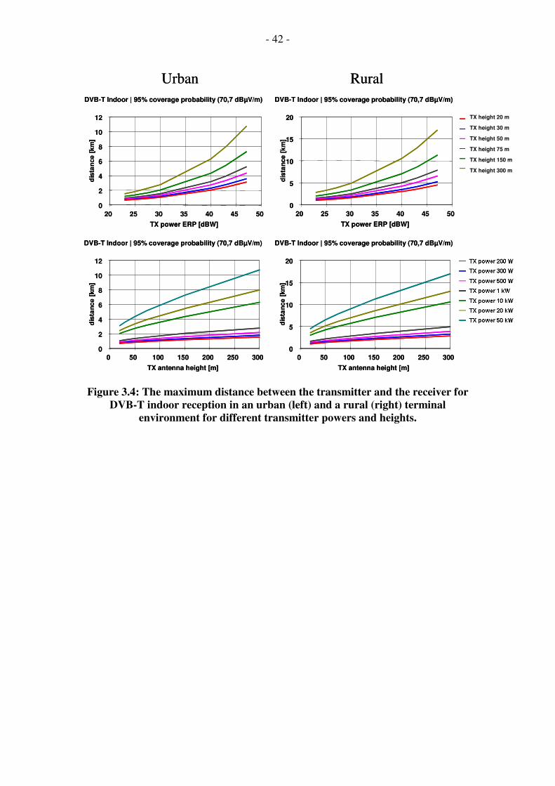
- 42 -


DVB-T indoor reception in an urban (left) and a rural (right) terminal

environment for different transmitter powers and heights.

TX height 20 m

TX height 30 m

TX height 50 m

TX height 75 m

TX height 150 m

TX height 300 m

0

2

4

6

8

10

12

20 25 30 35 40 45 50

TX power ERP [dBW]

DVB-T Indoor | 95% coverage probability (70,7 dBµV/m)

0

2

4

6

8

10

12

0 50 100 150 200 250 300



0

5

10

15

20

0 50 100 150 200 250 300



0

5

10

15

20

20 25 30 35 40 45 50

TX power ERP [dBW]


Urban Rural

TX height 20 m

TX height 30 m

TX height 50 m

TX height 75 m

TX height 150 m

TX height 300 m

TX height 20 m

TX height 30 m

TX height 50 m

TX height 75 m

TX height 150 m

TX height 300 m

0

2

4

6

8

10

12

20 25 30 35 40 45 50

TX power ERP [dBW]


0

2

4

6

8

10

12

0 50 100 150 200 250 300



0

5

10

15

20

0 50 100 150 200 250 300



0

5

10

15

20

20 25 30 35 40 45 50

TX power ERP [dBW]


Urban Rural

- 43 -


DVB-H, class A, reception in an urban (left) and a rural (right) terminal


TX height 20 m

TX height 30 m

TX height 50 m

TX height 75 m

TX height 150 m

TX height 300 m

0

5

10

15

20

0 50 100 150 200 250 300


DVB-H Class A | 95% coverage probability (62,6 dBµV/m)

0

5

10

15

20

20 25 30 35 40 45 50

TX power ERP [dBW]


0

5

10

15

20

25

30

20 25 30 35 40 45 50

TX power ERP [dBW]


0

5

10

15

20

25

30

0 50 100 150 200 250 300



Urban Rural

TX height 20 m

TX height 30 m

TX height 50 m

TX height 75 m

TX height 150 m

TX height 300 m

TX height 20 m

TX height 30 m

TX height 50 m

TX height 75 m

TX height 150 m

TX height 300 m

0

5

10

15

20

0 50 100 150 200 250 300



0

5

10

15

20

20 25 30 35 40 45 50

TX power ERP [dBW]


0

5

10

15

20

25

30

20 25 30 35 40 45 50

TX power ERP [dBW]


0

5

10

15

20

25

30

0 50 100 150 200 250 300



Urban Rural

- 44 -


DVB-H, class B, reception in an urban (left) and a rural (right) terminal


TX height 20 m

TX height 30 m

TX height 50 m

TX height 75 m

TX height 150 m

TX height 300 m

0

1

2

3

4

5

6

20 25 30 35 40 45 50

TX power ERP [dBW]

DVB-H Class B | 95% coverage probability (78,6 dBµV/m)

0

1

2

3

4

5

6

0 50 100 150 200 250 300



0

2

4

6

8

10

0 50 100 150 200 250 300



0

2

4

6

8

10

20 25 30 35 40 45 50

TX power ERP [dBW]


Urban Rural

TX height 20 m

TX height 30 m

TX height 50 m

TX height 75 m

TX height 150 m

TX height 300 m

TX height 20 m

TX height 30 m

TX height 50 m

TX height 75 m

TX height 150 m

TX height 300 m

0

1

2

3

4

5

6

20 25 30 35 40 45 50

TX power ERP [dBW]


0

1

2

3

4

5

6

0 50 100 150 200 250 300



0

2

4

6

8

10

0 50 100 150 200 250 300



0

2

4

6

8

10

20 25 30 35 40 45 50

TX power ERP [dBW]


Urban Rural

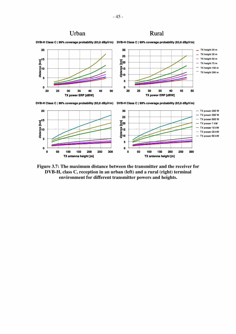
- 45 -


DVB-H, class C, reception in an urban (left) and a rural (right) terminal


TX height 20 m

TX height 30 m

TX height 50 m

TX height 75 m

TX height 150 m

TX height 300 m

0

5

10

15

20

20 25 30 35 40 45 50

TX power ERP [dBW]

DVB-H Class C | 99% coverage probability (63,6 dBµV/m)

0

5

10

15

20

0 50 100 150 200 250 300



0

5

10

15

20

25

30

20 25 30 35 40 45 50

TX power ERP [dBW]


0

5

10

15

20

25

30

0 50 100 150 200 250 300



Urban Rural

TX height 20 m

TX height 30 m

TX height 50 m

TX height 75 m

TX height 150 m

TX height 300 m

TX height 20 m

TX height 30 m

TX height 50 m

TX height 75 m

TX height 150 m

TX height 300 m

0

5

10

15

20

20 25 30 35 40 45 50

TX power ERP [dBW]


0

5

10

15

20

0 50 100 150 200 250 300



0

5

10

15

20

25

30

20 25 30 35 40 45 50

TX power ERP [dBW]


0

5

10

15

20

25

30

0 50 100 150 200 250 300



Urban Rural

- 46 -


DVB-H, class D, reception in an urban (left) and a rural (right) terminal


TX height 20 m

TX height 30 m

TX height 50 m

TX height 75 m

TX height 150 m

TX height 300 m

0

1

2

3

4

5

6

7

20 25 30 35 40 45 50

TX power ERP [dBW]

DVB-H Class D | 99% coverage probability (76,6 dBµV/m)

0

1

2

3

4

5

6

7

0 50 100 150 200 250 300



0

2

4

6

8

10

12

20 25 30 35 40 45 50

TX power ERP [dBW]


0

2

4

6

8

10

12

0 50 100 150 200 250 300



Urban Rural

TX height 20 m

TX height 30 m

TX height 50 m

TX height 75 m

TX height 150 m

TX height 300 m

TX height 20 m

TX height 30 m

TX height 50 m

TX height 75 m

TX height 150 m

TX height 300 m

0

1

2

3

4

5

6

7

20 25 30 35 40 45 50

TX power ERP [dBW]


0

1

2

3

4

5

6

7

0 50 100 150 200 250 300



0

2

4

6

8

10

12

20 25 30 35 40 45 50

TX power ERP [dBW]


0

2

4

6

8

10

12

0 50 100 150 200 250 300



Urban Rural

- 47 -

3.3 Coverage planning

To evaluate different transmitter network topologies, area coverage planning has to be

performed. As a reference area to be covered the Berlin area was chosen. As an

example of what can be reached with a single high power / high antenna transmitter

Figure 3.9 shows the coverage areas according the parameters given in Table 3.1.

θθθθθθθθθθθθθθθθθθθθθθθθθθθθθθθθθθθθθθθθθθθθθθθθθθθθθθθθθθθθθθθθθθθθθθθθθθθθθθθθθθθθθθθθθθθθθθθθθθθθθθθθθθθθθθθθθθθθθθθθθθθθθθθθθθθθθθθθθθθθθθθθθθθθθθθθθθθθθθθθθθθθθθθθθθθθθθθθθθθθθθθθθθθθθθθθθθθθθθθθθθθθθθθθθθθθθθθθθθθθθθθθθθθθθθθθθθθθθθθθθθθθθθθθθθθθθθθθθθθθθθθθθθθθθθθθθθθθθθθθθθθθθθθθθθθθθθθθθθθθθθθθθθθθθθθθθθθθθθθθθθθθθθθθθθθθθθθθθθθθθθθθθθθθθθθθθθθθθθθθθθθθθθθθθθθθθθθθθθθθθθθθθθθθθθ

kein Empfang

DVB-T Outdoor (58,94 dBµV/m)

Empfang möglich

DVB-H B (78,17 dBµV/m)

DVB-H D (76,63 dBµV/m)

DVB-T Indoor (70,27 dBµV/m)

DVB-H C (63,63 dBµV/m)

DVB-H A (62,84 dBµV/m)

BERLIN-WEST, STADT

BERLIN-OST, STADT

BERLIN ALEXANDERPLATZBERLIN ALEXANDERPLATZBERLIN ALEXANDERPLATZBERLIN ALEXANDERPLATZBERLIN ALEXANDERPLATZBERLIN ALEXANDERPLATZBERLIN ALEXANDERPLATZBERLIN ALEXANDERPLATZBERLIN ALEXANDERPLATZ

No reception possible


kein Empfang


Empfang möglich






BERLIN-WEST, STADT

BERLIN-OST, STADT




kein Empfang


Empfang möglich






BERLIN-WEST, STADT

BERLIN-OST, STADT



Figure 3.9: Coverage by single transmitter, height: 300 m, power: 20 kW, for

different reception modes, for the parameters see Table 3.1.

One major application of DVB-H is expected to be IP datacast delivery technology in

conjunction with a mobile telecommunications network like GPRS or UMTS.

Therefore, it is of interest to know how the cellular layout of DVB-H cells can be

adapted from the typical broadcast cell layout with high antennas, high power

transmitters with wide coverage range towards the typical layout of low height, low

power sites with small cell ranges of mobile telecommunication networks. Of

particular interest is the question of whether or not the cositing of DVB-H transmitters

with mobile radio sites is feasible. Within this chapter these questions are only treated

from the radio network perspective. It should be mentioned that the necessary feeding

of the DVB-H transmitters, which could be far too costly for a high density of

transmitters within an area to be covered, is outside of the scope of this chapter.

3.3.1 Single frequency networks (SFN)

For comparison purposes a reference coverage area was defined as a circle of 20 km

around Berlin Alexanderplatz corresponding to an area of approx. 1250 km2. For

DVB-H, class A reception, a coverage probability of at least 95 % is reached for

nearly all pixels within this area with a single 300 m high transmitter at a power level

of 20 kW ERP with respect to the parameters of Table 3.1, column 3. The coverage

probability for this single transmitter reference network is given in Figure 3.10.

- 48 -

Figure 3.10: Coverage probability of a single DVB-H transmitter (300 m high, 20

kW), in 8k mode, 16-QAM, inner code rate 2/3, for class A reception. The circle

is of 20 km radius around transmitter site.

Attempts were made to achieve at least the same coverage area as enclosed by the

circle of 20 km radius around Berlin Alexanderplatz at a coverage probability of 95 %

as depicted in Figure 3.10 by different regular single frequency network topologies.

Different heights of the transmitter antennas as well as different distances between the

transmitters were specified in advance. Then the transmitter powers - equal for each

transmitter of the SFN – were adjusted to achieve the target coverage within the

circular area around Berlin Alexanderplatz comparable to the single transmitter

reference. The superposition method for single frequency network coverage

calculation used in this study is the log-normal method [1], see also Appendix 3.

Figure 3.11 shows the coverage probability for a SFN consisting of 19 transmitters

each with 150 m high antennas with a distance of 10 km between the transmitters. The

power necessary at each transmitter is 400 W to achieve approximately the same

coverage area as the single transmitter reference. Thus, the power sum of all the

transmitters is 19 x 400 W = 7.6 kW. If the antenna height is lowered to 75 m a

transmitter power of 1.25 kW is needed to cover the same area. Figure 3.12 shows the

coverage probability for a SFN consisting of 19 transmitters with a distance of 10 km

between the transmitters and a transmitter power sum of 19 x 1.25 kW = 23.75 kW.

If the network is densified to a distance of 5 km between the transmitters, 61

transmitters fall into a circle of 20 km radius. In Figure 3.13 the coverage probability

is shown in this case where each transmitter is at a height of 75 m was and the power

at each transmitter is 100 W. The power sum is 61 x 100 W = 6.1 kW for this

topology.

- 49 -

Figure 3.11: SFN for DVB-H, class A reception, 8 k FFT mode, guard interval

1/8, 16-QAM, inner code rate 2/3, TX height 150 m, TX distance 10 km, TX

power 400 W.


1/8, 16-QAM, inner code rate 2/3, TX height 75 m, TX distance 10 km, TX power

1.25 kW.

- 50 -



100 W.



200 W.

- 51 -

In Figure 3.14 the coverage area for the SFN with a distance between transmitters of 5

km and the transmitters at a height of 50 m is shown. A transmitter power of 200 W is

necessary to achieve the target coverage within the circular area around Berlin

Alexanderplatz comparable to the single transmitter reference. Therefore, the overall

transmitter power is 61 x 200 W = 12.2 kW.

If the topology is densified further, transmitter heights and distances closer to those of

mobile telecommunication networks are possible. Figure 3.15 depicts the coverage

probability for a distance of 2.5 km between the transmitters and an antenna height of

20 m. A power of 50 W per transmitter is necessary. The number of transmitters is

241 and thus the power sum is 241 x 50 W = 12 kW.


1/8, 16-QAM, inner code rate 2/3, TX height 20 m, TX distance 2.5 km, TX

power 50 W.

One major issue in SFN topologies is self-interference which is strongly related to the

choice of OFDM symbol and guard interval length. Therefore, the guard interval

length for different OFDM modes was varied and its impact on coverage was

investigated. As a synchronisation strategy in the receiver it is assumed that the

received power of the nearest transmitter is set at the beginning of the guard interval.

In comparison to Figure 3.13 the coverage probability plot shown in Figure 3.16 is

based on the same parameters except for the guard interval length which was

shortened from 1/8 to 1/32 (28 µs). Obviously, self-interference is of no consequence

for transmitter distances of 5 km even for this short guard interval.

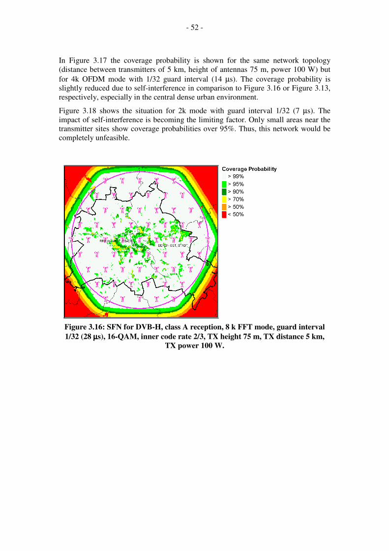
- 52 -

In Figure 3.17 the coverage probability is shown for the same network topology

(distance between transmitters of 5 km, height of antennas 75 m, power 100 W) but

for 4k OFDM mode with 1/32 guard interval (14 µs). The coverage probability is

slightly reduced due to self-interference in comparison to Figure 3.16 or Figure 3.13,

respectively, especially in the central dense urban environment.

Figure 3.18 shows the situation for 2k mode with guard interval 1/32 (7 µs). The

impact of self-interference is becoming the limiting factor. Only small areas near the

transmitter sites show coverage probabilities over 95%. Thus, this network would be

completely unfeasible.


1/32 (28 µµµµs), 16-QAM, inner code rate 2/3, TX height 75 m, TX distance 5 km,

TX power 100 W.

- 53 -


1/32 (14 µµµµs), 16-QAM, inner code rate 2/3, TX height 75 m, TX distance 5 km,

TX power 100 W.


1/32 (7 µµµµs), 16-QAM, inner code rate 2/3, TX height 75 m, TX distance 5 km, TX

power 100 W.

- 54 -

The main findings in this subsection are:

• “Large” SFNs with low power, low height transmitters are possible. Care has

to be taken in choosing the guard interval length in relation to the distance

between the transmitters.

• The sum of transmit powers of all transmitters of the SFN in comparison to a

single transmitter covering the same area is remarkable lower even for

significantly lower antennas within the SFN.

• Further optimization has to be done related to the distribution of the sum

power of the SFN, e.g. from Figure 3.13 it can be seen that coverage

probability could be enhanced in the central part of the network located in a

densely built up urban environment. Thus, one approach could be to increase

the transmit power of the central transmitters at the expense of decreasing

transmit power for the outer transmitters of the SFN.

3.3.2 Multi frequency networks (MFN)

3.3.2.1 Omni-directional antennas

To evaluate network topologies closer to those of mobile telecommunications

networks multi frequency networks with different cluster sizes for omni-directional as

well as for sectorized antenna patterns are analyzed in this subsection.

The basis for the investigation is a hexagonal cell layout with cell cluster size N

where N = I2 + IJ + J

2, and I, J are integers.

The Euclidian distance between the centres of two co-channel cells is D and the range

of each cell is R.

The normalized re-use distance is Q = D/R = sqrt (3 N).

For different cluster sizes it follows that:

N I J Q

1 1 0 1.73

3 1 1 3.00

4 2 0 3.46

7 2 1 4.58

9 3 0 5.20

12 2 2 6.00

13 3 1 6.24

16 4 0 6.93

19 3 2 7.55

21 4 1 7.94

27 3 3 9.00

Table 3.2: Normalized re-use distance Q as function of cluster size N (or integers

I, J).

To estimate the inference power different methods were applied to determine the

distance from the 6 interferers of the first ring for a location at the border of the

central serving cell:

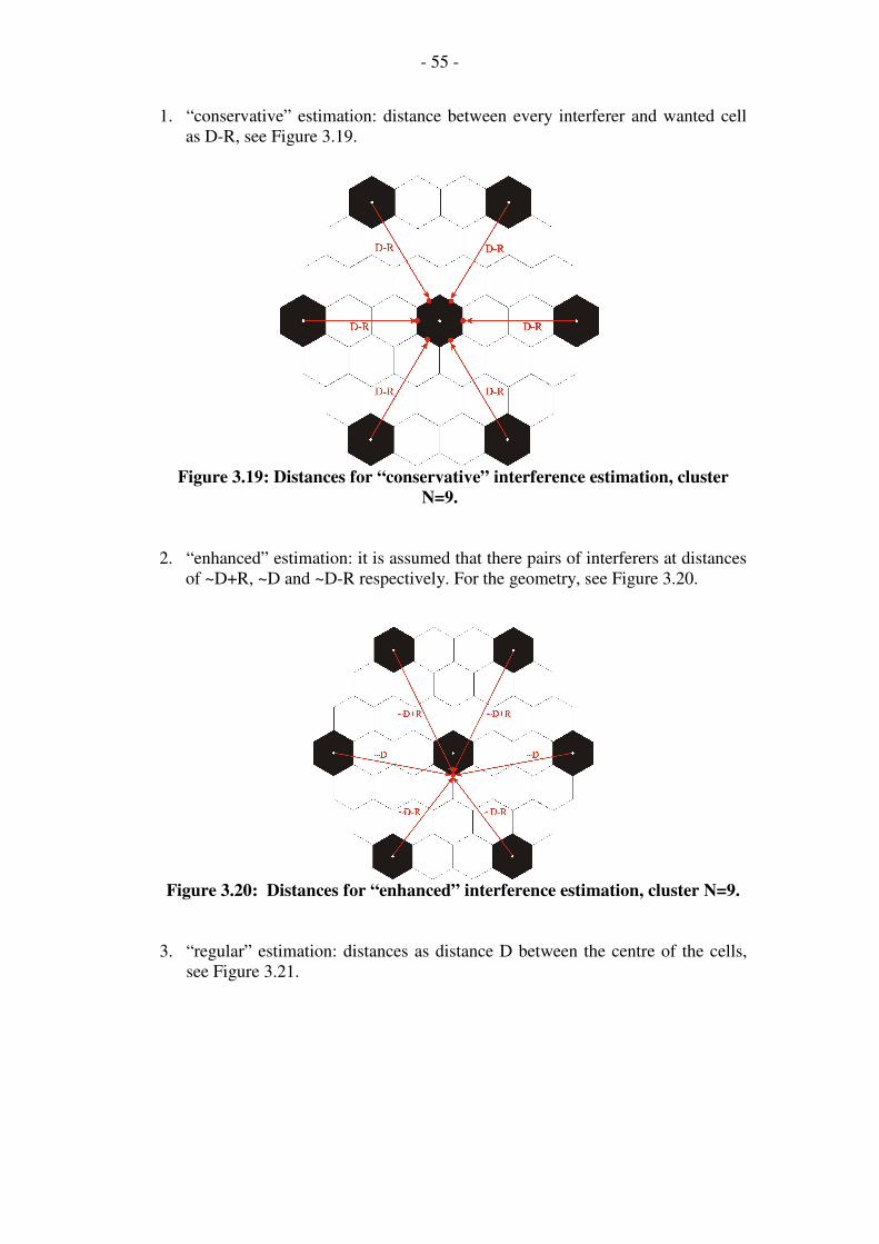
- 55 -

1. “conservative” estimation: distance between every interferer and wanted cell

as D-R, see Figure 3.19.

Figure 3.19: Distances for “conservative” interference estimation, cluster

N=9.

2. “enhanced” estimation: it is assumed that there pairs of interferers at distances

of ~D+R, ~D and ~D-R respectively. For the geometry, see Figure 3.20.

Figure 3.20: Distances for “enhanced” interference estimation, cluster N=9.

3. “regular” estimation: distances as distance D between the centre of the cells,

see Figure 3.21.

- 56 -

Figure 3.21: Distances for “regular” interference estimation, cluster N=9.

4. “optimistic” estimation: distance for all interference sources D+R, see Figure

3.22.

Figure 3.22: Distances for “optimistic” interference estimation, cluster N=9.

Based on the aforementioned estimation methods to take into account the interference

power from co-channel cells as a function of distance, C/I values were calculated on

the basis of ITU-R P.1546-1 curves for different cluster sizes, transmitter antenna

heights and cell ranges R. For a rural environment with cell radii of R = 5 km and R =

2.5 km as well as for an urban environment with cell radii of R = 2.5 km and R = 1.25

km the achieved C/I values were calculated.

In Table 3.3 the achieved C/I values when taking into account the first ring of

interferers around a central cell are shown for different cluster sizes N as well as for

different transmitter antenna heights for an urban environment where a cell radius of

R = 2.5 km is assumed.

- 57 -

"conservative" estimation

TX height [m] / cluster N 3 4 7 9 12 13 16 19 21

20 4,34 8,38 15,94 19,23 22,89 23,90 26,46 28,55 29,75

30 3,52 7,27 14,39 17,55 21,12 22,11 24,64 26,72 27,92

50 2,68 6,09 12,62 15,57 18,95 19,89 22,34 24,38 25,56

75 2,14 5,29 11,33 14,07 17,27 18,17 20,52 22,50 23,66

150 1,42 4,28 9,61 12,00 14,79 15,58 17,68 19,46 20,52

300 0,68 3,27 8,03 10,12 12,52 13,20 14,99 16,52 17,43

"enhanced" estimation


20 8,41 12,21 19,26 22,30 25,68 26,61 28,97 30,90 32,01

30 7,48 11,00 17,65 20,58 23,89 24,80 27,15 29,08 30,19

50 6,49 9,67 15,76 18,50 21,65 22,53 24,82 26,72 27,83

75 5,81 8,74 14,35 16,92 19,91 20,75 22,96 24,83 25,92

150 4,89 7,49 12,38 14,61 17,23 17,98 19,96 21,66 22,68

300 3,96 6,27 10,55 12,47 14,71 15,35 17,04 18,51 19,39

"regular" estimation

TX height [m] / cluster 3 4 7 9 12 13 16 19 21

20 12,31 15,25 21,07 23,70 26,72 27,55 29,73 31,52 32,56

30 10,95 13,74 19,34 21,91 24,89 25,73 27,90 29,70 30,75

50 9,45 12,01 17,25 19,70 22,59 23,40 25,53 27,32 28,37

75 8,40 10,76 15,66 17,99 20,76 21,55 23,63 25,40 26,44

150 7,04 9,12 13,38 15,42 17,89 18,60 20,49 22,12 23,10

300 5,75 7,59 11,31 13,07 15,17 15,78 17,41 18,83 19,68

"optimistic" estimation


20 18,23 20,52 25,20 27,39 29,94 30,66 32,53 34,09 35,00

30 16,59 18,80 23,39 25,56 28,11 28,83 30,72 32,31 33,24

50 14,66 16,74 21,13 23,24 25,75 26,46 28,35 29,96 30,91

75 13,22 15,18 19,36 21,40 23,84 24,55 26,42 28,04 28,99

150 11,26 12,97 16,63 18,46 20,69 21,33 23,08 24,64 25,56

300 9,47 10,95 14,10 15,66 17,58 18,14 19,66 21,06 21,88

Table 3.3: Achieved C/I in dB as function of cluster size N and TX antenna

height in an urban environment, R = 2.5 km, based on the ITU-R P.1546-1

propagation model.

The yellow fields in Table 3.3 mark where a C/I of at least 26.2 dB is achieved which

would be sufficient for a protection ratio of 14.2 dB + 3 dB = 17.2 dB as in case of

DVB-T with 16-QAM, code rate 2/3 reception and DVB-T as the interfering signal.

An additional location correction of 9 dB for 95 % coverage probability leads to a

required C/I of 26.2 dB.

Table 3.4 shows the resultant C/I values for R = 1.25 km under the same conditions as

for Table 3.3. Again the yellow fields in Table 3.4 mark where a C/I of at least 26.2

dB is achieved which would be sufficient for a protection ratio of 14.2 dB + 3 dB =

17.2 dB as in case of DVB-T with 16-QAM, code rate 2/3 reception and DVB-T as

the interfering signal. An additional location correction of 9 dB for 95 % coverage

probability leads to a required C/I of 26.2 dB.

- 58 -



20 3,03 6,46 13,11 16,07 19,47 20,42 22,88 24,91 26,09

30 2,59 5,83 12,01 14,75 17,91 18,80 21,10 23,01 24,14

50 2,11 5,16 10,85 13,35 16,23 17,03 19,14 20,89 21,93

75 1,79 4,71 10,09 12,42 15,09 15,83 17,77 19,39 20,35

150 1,21 3,95 8,93 11,07 13,47 14,14 15,86 17,29 18,13

300 0,70 3,22 7,80 9,75 11,93 12,53 14,07 15,35 16,09



20 6,86 10,07 16,26 19,02 22,18 23,06 25,35 27,24 28,34

30 6,31 9,31 15,02 17,57 20,51 21,33 23,48 25,27 26,32

50 5,70 8,48 13,69 16,00 18,67 19,41 21,38 23,03 24,00

75 5,28 7,93 12,80 14,93 17,39 18,08 19,89 21,42 22,32

150 4,58 7,02 11,47 13,40 15,59 16,19 17,79 19,12 19,90

300 3,92 6,14 10,18 11,92 13,88 14,42 15,83 17,00 17,69



20 9,89 12,48 17,77 20,24 23,12 23,93 26,06 27,83 28,87

30 9,03 11,43 16,32 18,62 21,33 22,09 24,11 25,81 26,80

50 8,12 10,33 14,78 16,88 19,35 20,05 21,91 23,48 24,41

75 7,52 9,60 13,75 15,69 17,97 18,61 20,33 21,79 22,66

150 6,56 8,48 12,27 14,01 16,03 16,60 18,11 19,39 20,14

300 5,63 7,39 10,84 12,41 14,23 14,74 16,07 17,19 17,85



20 15,14 17,26 21,66 23,77 26,27 26,98 28,85 30,42 31,35

30 13,89 15,85 19,95 21,94 24,31 24,99 26,78 28,30 29,20

50 12,57 14,36 18,09 19,91 22,09 22,72 24,38 25,81 26,66

75 11,70 13,36 16,81 18,49 20,50 21,08 22,64 23,97 24,77

150 10,41 11,91 15,01 16,49 18,26 18,77 20,12 21,29 21,98

300 9,15 10,52 13,31 14,64 16,20 16,65 17,84 18,85 19,45

Table 3.4: achieved C/I in dB as function of cluster size N and TX antenna height

in an urban environment, R = 1.25 km, based on the ITU-R P.1546-1

propagation model.

Comparison of Table 3.3 with Table 3.4 shows that for lower transmitter antenna

heights a lower reuse distance is needed. It can also be seen that for smaller cell sizes

a higher reuse distance and thus more frequencies are needed.

Table 3.5 shows the calculated C/I values for different cluster sizes N as well as for

different transmitter antenna heights for a rural environment where a cell radius of R

= 5 km is assumed. The yellow fields in Table 3.5 mark where a C/I of at least 26.2





In Table 3.6 the calculated C/I values for different cluster sizes N as well as for

different transmitter antenna heights for a rural environment where a cell radius of R

= 2.5 km is assumed. The yellow fields in Table 3.6 mark where a C/I of at least 26.2





Comparison of Table 3.5 with Table 3.6 shows again that for lower transmitter

antenna heights a lower reuse distance is needed. Also again it can be seen that for

smaller cell sizes a higher reuse distance and thus more frequencies are needed. Table

3.3 for an urban environment compared to Table 3.6 for a rural environment but for

the same radius R shows that there is only a negligible difference in required reuse

distance and thus frequencies for the above mentioned example where a C/I of 26.2

dB is required for 95 % coverage probability in different environments are considered.

- 59 -



20 6,12 10,49 18,33 21,61 25,21 26,18 28,66 30,66 31,81

30 5,31 9,55 17,33 20,65 24,34 25,35 27,94 30,06 31,28

50 4,23 8,24 15,82 19,16 22,91 23,96 26,66 28,92 30,23

75 3,36 7,14 14,48 17,80 21,58 22,67 25,44 27,80 29,16

150 2,17 5,49 12,08 15,22 18,87 19,96 22,75 25,19 26,61

300 1,25 4,14 9,83 12,60 15,88 16,91 19,53 21,89 23,28



20 10,23 14,33 21,58 24,59 27,89 28,78 31,05 32,88 33,93

30 9,38 13,37 20,61 23,68 27,09 28,03 30,43 32,39 33,53

50 8,24 12,03 19,12 22,23 25,74 26,73 29,27 31,39 32,62

75 7,29 10,87 17,78 20,90 24,47 25,49 28,13 30,36 31,66

150 5,90 9,04 15,31 18,28 21,78 22,83 25,51 27,87 29,24

300 4,73 7,43 12,85 15,50 18,69 19,69 22,25 24,57 25,93



20 14,62 17,63 23,42 25,99 28,91 29,71 31,78 33,48 34,47

30 13,62 16,62 22,50 25,15 28,19 29,04 31,25 33,09 34,16

50 12,17 15,12 21,04 23,76 26,93 27,84 30,20 32,19 33,36

75 10,91 13,79 19,70 22,45 25,71 26,66 29,13 31,25 32,49

150 8,83 11,45 17,05 19,75 23,03 24,02 26,58 28,84 30,16

300 7,02 9,28 14,25 16,71 19,78 20,75 23,24 25,51 26,84



20 20,62 22,88 27,45 29,55 31,99 32,67 34,45 35,92 36,79

30 19,64 21,95 26,67 28,88 31,47 32,21 34,14 35,76 36,71

50 18,13 20,48 25,34 27,66 30,43 31,23 33,33 35,13 36,19

75 16,77 19,14 24,08 26,48 29,37 30,23 32,46 34,38 35,52

150 14,22 16,51 21,38 23,82 26,83 27,74 30,13 32,23 33,48

300 11,70 13,76 18,24 20,56 23,49 24,41 26,81 28,99 30,27

Table 3.5: achieved C/I in dB as function of cluster size N and TX antenna

height in a rural environment, R = 5 km, based on the ITU-R P.1546-1

propagation model. "conservative" estimation


20 4,36 8,41 15,98 19,27 22,94 23,94 26,51 28,60 29,80

30 3,56 7,32 14,45 17,61 21,19 22,17 24,71 26,79 27,99

50 2,75 6,17 12,72 15,67 19,06 20,00 22,46 24,50 25,68

75 2,25 5,42 11,48 14,24 17,44 18,34 20,71 22,68 23,85

150 1,65 4,55 9,94 12,35 15,16 15,95 18,05 19,84 20,91

300 1,19 3,87 8,75 10,88 13,32 14,00 15,81 17,36 18,28



20 8,37 12,18 19,24 22,28 25,66 26,59 28,96 30,88 31,99

30 7,46 10,99 17,65 20,58 23,89 24,80 27,16 29,08 30,20

50 6,50 9,70 15,80 18,55 21,71 22,59 24,88 26,78 27,89

75 5,86 8,81 14,45 17,02 20,02 20,86 23,08 24,95 26,04

150 5,08 7,71 12,66 14,90 17,54 18,29 20,28 21,99 23,00

300 4,45 6,84 11,23 13,18 15,45 16,09 17,81 19,29 20,18



20 12,35 15,29 21,11 23,74 26,76 27,60 29,77 31,56 32,60

30 11,01 13,80 19,40 21,98 24,96 25,80 27,97 29,77 30,82

50 9,55 12,11 17,36 19,82 22,70 23,52 25,65 27,44 28,50

75 8,55 10,92 15,83 18,16 20,94 21,73 23,82 25,59 26,63

150 7,34 9,44 13,74 15,79 18,26 18,98 20,88 22,52 23,50

300 6,42 8,31 12,09 13,86 15,99 16,61 18,25 19,68 20,54



20 18,27 20,56 25,25 27,44 29,99 30,71 32,58 34,13 35,05

30 16,65 18,87 23,46 25,63 28,18 28,90 30,79 32,38 33,32

50 14,76 16,85 21,25 23,36 25,87 26,58 28,47 30,09 31,04

75 13,39 15,35 19,54 21,58 24,03 24,73 26,61 28,23 29,19

150 11,61 13,32 17,01 18,84 21,08 21,73 23,48 25,04 25,96

300 10,22 11,72 14,91 16,49 18,42 18,99 20,52 21,92 22,75


in a rural environment, R = 2.5 km, based on the ITU-R P.1546-1 propagation

model.

- 60 -

3.3.3 Sectorized cell layout

In mobile telecommunication networks sectorizing of cells is applied to increase

capacity without additional base station locations. In order to investigate network

topologies for DVB-H that are similar to mobile telecommunication network

topologies in this subsection sectorization of hexagonal cells into 6 x 60° sector and 3

x 120° is considered.

In Figure 3.23 the interferer’s distances for 60° and 120° sectorization are depicted. It

should be noted that in case of 120° sectorization only 2 interferers have to be

considered and for 60° sectorization only 1 interferer has to be taken into account

from the first ring around the serving cell.

Figure 3.23: Distances for the interference calculation for 60° sectorization (left)

and 120° sectorization (right).

Based on the geometry of Figure 3.23, in Table 3.7 the achieved C/I values as a

function of cluster size and TX antenna height in an urban environment are given for

a cell range of 2.5 km.

The yellow fields in Table 3.7 mark where a C/I of at least 26.2 dB is achieved which

would be sufficient for a protection ratio of 14.2 dB + 3 dB = 17.2 dB as in the case of

DVB-T with 16-QAM, code rate 2/3 reception and DVB-T as the interfering signal.

An additional location correction of 9 dB for 95 % coverage probability leads to a


- 61 -

120° sectors


20 18,72 21,52 27,08 29,60 32,49 33,30 35,39 37,11 38,11

30 17,30 19,96 25,33 27,80 30,66 31,47 33,56 35,30 36,32

50 15,71 18,16 23,19 25,56 28,34 29,13 31,19 32,93 33,95

75 14,57 16,84 21,55 23,81 26,49 27,26 29,28 31,00 32,03

150 13,07 15,06 19,16 21,14 23,54 24,23 26,08 27,69 28,66

300 11,66 13,41 16,97 18,66 20,71 21,31 22,90 24,31 25,16

60° sectors


20 24,39 26,85 31,83 34,13 36,81 37,56 39,51 41,13 42,08

30 22,82 25,18 30,03 32,31 34,98 35,73 37,69 39,34 40,31

50 21,00 23,20 27,81 30,02 32,62 33,36 35,32 36,98 37,96

75 19,66 21,72 26,08 28,20 30,74 31,47 33,39 35,05 36,04

150 17,87 19,67 23,48 25,36 27,65 28,32 30,11 31,68 32,63

300 16,23 17,80 21,09 22,69 24,66 25,23 26,78 28,17 29,03


in an urban environment for 60° and 120° sectorized cells, R = 2.5 km, based on

the ITU-R P.1546-1 propagation model.

For a decreased cell range of R = 1.25 km Table 3.8 shows C/I values in case of

sectorization for an urban environment as a function of TX antenna height and cluster

size N.

Again the yellow fields mark where a C/I of at least 26.2 dB is achieved which would

be sufficient for a protection ratio of 14.2 dB + 3 dB = 17.2 dB as in case of DVB-T

with 16-QAM, code rate 2/3 reception and DVB-T as the interfering signal. An

additional location correction of 9 dB for 95 % coverage probability leads to a


120° sectors


20 16,16 18,64 23,72 26,09 28,87 29,66 31,71 33,43 34,44

30 15,22 17,51 22,20 24,42 27,03 27,77 29,73 31,37 32,34

50 14,21 16,31 20,58 22,60 24,99 25,67 27,47 29,00 29,90

75 13,55 15,52 19,48 21,34 23,55 24,18 25,85 27,27 28,11

150 12,51 14,32 17,92 19,58 21,53 22,08 23,54 24,78 25,51

300 11,50 13,15 16,41 17,91 19,65 20,14 21,43 22,51 23,15

60° sectors


20 21,48 23,70 28,35 30,55 33,15 33,89 35,83 37,46 38,41

30 20,34 22,39 26,71 28,78 31,24 31,94 33,79 35,36 36,29

50 19,14 21,01 24,94 26,82 29,08 29,73 31,45 32,92 33,79

75 18,34 20,09 23,73 25,47 27,55 28,15 29,75 31,12 31,93

150 17,15 18,75 22,02 23,57 25,40 25,93 27,32 28,52 29,23

300 15,98 17,44 20,40 21,79 23,42 23,88 25,11 26,15 26,76


in an urban environment for 60° and 120° sectorized cells, R = 1.25 km, based on

the ITU-R P.1546-1 propagation model.

Inspection of Table 3.7 and Table 3.8 reveals that for a smaller sector and lower TX

antenna the cluster size can be smaller for a given C/I that should be achieved. Similar

results to those in Table 3.7 and Table 3.8 are obtained in the case of a rural

environment.

It should be noted that the cluster sizes given in Table 3.7 and Table 3.8 may be too

optimistic, because ideal sector antennas are assumed with infinite front-to-back /

front-to-side ratio.

- 62 -

Although the cluster size N can be considerably lowered by sectorizing the hexagonal

cells into 120° or even into 60° sectors to achieve a given C/I that does not mean that

a lower number of frequencies is needed to provide area coverage. This is due to the

fact that the required total number of frequencies is the cluster size times the number

of sectors. Therefore e.g. in case of 120° sectoring of cells the number of required

frequencies is 3 x N and in case of 60° sectors 6 x N frequencies will be needed. An

example should make this clear:

For an urban environment, a cell radius of 2.5 km and a TX antenna height of 20 m,

from Table 3.3 it can be seen that in case of a non-sectorized cell layout a cluster size

of N = 16 is needed to fulfil the C/I requirement of 26.2 dB. In Table 3.7 a

corresponding value for the cluster size in case of 120° sectorization is given as N = 7.

In fact this value has to be multiplied by 3 to give the number of frequencies needed

which is thus higher than in case of non-sectorized cells. Therefore, for broadcast

applications where capacity is of no concern sectorization seems not to be an adequate

way to lower the frequency needs for area coverage.

3.3.4 Antenna down-tilting

Taking into account the elevation pattern of a directional antenna leads to the idea of

down-tilting the antennas of the radio network’s transmitters. This approach is heavily

used in mobile telecommunications networks especially in small cells to effectively

lower the cell range in areas were high capacity is demanded and to have a sharp

transition at the cell border with the neighbouring cells.

In Figure 3.24 the assumed cos2 shaped elevation antenna diagram and the geometry

for C/I calculation is given.

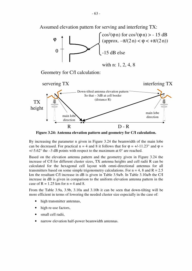
- 63 -

TX

height

0

ϕ

0

ϕcos2(ϕ.n) for cos2(ϕ.n) > - 15 dB

(approx. –π/(2.n) < ϕ < +π/(2.n))

-15 dB else

with n: 1, 2, 4, 8

Assumed elevation pattern for serving and interfering TX:

Geometry for C/I calculation:

Down-tilted antenna elevation pattern

So that – 3dB at cell border

(distance R)

R D - R

main lobe

directionmain lobe

direction

servering TX interfering TX

Figure 3.24: Antenna elevation pattern and geometry for C/I calculation.

By increasing the parameter n given in Figure 3.24 the beamwidth of the main lobe

can be decreased. For practical n = 4 and 8 it follows that for ϕ = +/-11.23° and ϕ =

+/-5.62° the –3 dB points with respect to the maximum at 0° are reached.

Based on the elevation antenna pattern and the geometry given in Figure 3.24 the

increase of C/I for different cluster sizes, TX antenna heights and cell radii R can be

calculated for the hexagonal cell layout with omni-directional antennas for all

transmitters based on some simple trigonometry calculations. For n = 4, 8 and R = 2.5

km the resultant C/I increase in dB is given in Table 3.9a/b. In Table 3.10a/b the C/I

increase in dB is given in comparison to the uniform elevation antenna pattern in the

case of R = 1.25 km for n = 4 and 8.

From the Table 3.9a, 3.9b, 3.10a and 3.10b it can be seen that down-tilting will be

more efficient in terms of lowering the needed cluster size especially in the case of:

• high transmitter antennas,

• high re-use factors,

• small cell radii,

• narrow elevation half-power beamwidth antennas.

- 64 -


20 0,14 0,17 0,20 0,22 0,23 0,23 0,24 0,24 0,24

30 0,21 0,25 0,31 0,33 0,35 0,35 0,36 0,37 0,37

50 0,36 0,43 0,53 0,56 0,59 0,60 0,62 0,63 0,64

75 0,55 0,66 0,82 0,87 0,92 0,93 0,96 0,98 0,99

150 1,17 1,43 1,79 1,91 2,03 2,06 2,13 2,18 2,20

300 2,66 3,33 4,36 4,73 5,09 5,18 5,40 5,57 5,66

Table 3.9a: Increase of C/I in [dB] by down-tilting for n = 4 and R = 2.5 km.

Table 3.9b: Increase of C/I in [dB] by down-tilting for n = 8 and R = 2.5 km.


20 0,29 0,34 0,42 0,44 0,47 0,47 0,49 0,50 0,50

30 0,44 0,52 0,64 0,68 0,72 0,73 0,75 0,77 0,77

50 0,75 0,91 1,12 1,20 1,26 1,28 1,32 1,35 1,37

75 1,17 1,43 1,79 1,91 2,03 2,06 2,13 2,18 2,20

150 2,66 3,33 4,36 4,73 5,09 5,18 5,40 5,57 5,66

300 6,99 9,74 12,00 12,00 12,00 12,00 12,00 12,00 12,00

Table 3.10a: Increase of C/I in [dB] by down-tilting for n = 4 and R = 1.25 km. TX height [m] / cluster 3 4 7 9 12 13 16 19 21

20 0,59 0,71 0,88 0,93 0,98 1,00 1,03 1,05 1,06

30 0,92 1,11 1,38 1,47 1,56 1,58 1,63 1,67 1,69

50 1,63 2,01 2,55 2,73 2,91 2,96 3,06 3,14 3,18

75 2,68 3,36 4,39 4,76 5,13 5,22 5,44 5,60 5,69

150 7,30 10,20 12,00 12,00 12,00 12,00 12,00 12,00 12,00

300 12,00 12,00 12,00 12,00 12,00 12,00 12,00 12,00 12,00

Table 3.10b: Increase of C/I in [dB] by down-tilting for n = 8 and R = 1.25 km.

The increase in C/I given in Table 3.9a, 3.9b, 3.10a and 3.10b can be directly added to

the absolute C/I values given in the tables of the previous subsections corresponding

to the proper radii.

Thus antenna down-tilting is an efficient means to lower the required frequency reuse

or cluster size, respectively. But a prerequisite is the realization of a narrow half-

power beamwidth antenna pattern in elevation which leads to relatively large antennas

due to the low frequencies under consideration for DVB-T/-H in comparison to

mobile telecommunications frequencies.

3.3.5 Illumination of MFN cells by SFNs

Combining the benefits of SFNs with the cellular layout of MFNs to distribute more

localized content leads to the idea of illuminating the hexagonal cell area by an SFN

whose transmitters are located in the corners of the hexagon. In this subsection the

analysis is restricted to the case where only 3 transmitters with 120° sector antennas in

every second corner of the hexagonal cell are used to illuminate the cell area. This

case is the most preferable due to the fact that if only 3 sectorized transmitters are used

to form the SFN no more transmitter locations are needed that in the case where

omnidirectional antennas in the centre of the cell are used.


20 0,29 0,34 0,42 0,44 0,47 0,47 0,49 0,50 0,50

30 0,44 0,52 0,64 0,68 0,72 0,73 0,75 0,77 0,77

50 0,75 0,91 1,12 1,20 1,26 1,28 1,32 1,35 1,37

75 1,18 1,43 1,79 1,92 2,03 2,06 2,13 2,18 2,21

150 2,68 3,36 4,39 4,76 5,13 5,22 5,44 5,60 5,69

300 7,30 10,20 12,00 12,00 12,00 12,00 12,00 12,00 12,00

- 65 -

In Figure 3.25 the geometry of the cell layout is depicted and the distances for C/I

calculation are given.

Figure 3.25: Geometry for C/I calculation when illuminating the MFN cells by 3

transmitter SFNs.

For the point on the cell border of the central cell under consideration in Figure 3.25

the serving part of the received power is delivered by two transmitters at a distance of

R and one transmitter at a distance of 2R. The interference power comes from the

sectorized antennas of the first ring of cells using the same frequency and is given by

two transmitters at a distance of ~D+2R, two transmitters at a distance of ~D+R and

another two transmitters at distance ~D.

Table 3.11 to Table 3.14 show the achieved C/I with 3 transmitter SFNs for

illuminating the MFN cells for different cluster sizes, TX antenna heights, cell radii R

and environments based on calculations according to the ITU-R P.1546-1 model.

Again the yellow fields in these tables mark where a C/I of at least 26.2 dB is

achieved which would be sufficient for a protection ratio of 14.2 dB + 3 dB = 17.2 dB

as in case of DVB-T with 16-QAM, code rate 2/3 reception and DVB-T as the

interfering signal. An additional location correction of 9 dB for 95 % coverage


- 66 -


20 22,74 25,51 30,82 33,17 35,84 36,58 38,48 40,04 40,95

30 21,78 24,57 30,01 32,45 35,27 36,06 38,12 39,83 40,83

50 20,37 23,14 28,66 31,20 34,18 35,04 37,26 39,14 40,25

75 19,14 21,86 27,41 30,02 33,11 34,01 36,36 38,37 39,55

150 17,01 19,51 24,85 27,43 30,59 31,54 34,02 36,19 37,48

300 15,04 17,22 21,99 24,39 27,40 28,34 30,79 33,01 34,32

Table 3.11: Achieved C/I for MFN hexagonal layout with SFN illumination of

cells by 3 x 120° sectors for R = 5 km and a rural environment based on the ITU-

R P.1546-1 propagation model. TX height [m] / cluster 3 4 7 9 12 13 16 19 21

20 20,52 23,26 28,63 31,06 33,85 34,62 36,62 38,28 39,24

30 19,15 21,75 26,95 29,33 32,10 32,87 34,88 36,56 37,54

50 17,61 20,00 24,89 27,18 29,87 30,63 32,63 34,31 35,30

75 16,51 18,72 23,31 25,50 28,11 28,85 30,82 32,49 33,48

150 15,12 17,05 21,06 22,99 25,33 26,02 27,83 29,41 30,35

300 14,02 15,73 19,20 20,87 22,88 23,47 25,05 26,44 27,27


cells by 3 x 120° sectors for R = 2.5 km and a rural environment based on the

ITU-R P.1546-1 propagation model. TX height [m] / cluster 3 4 7 9 12 13 16 19 21

20 20,55 23,28 28,66 31,08 33,86 34,64 36,64 38,29 39,26

30 19,16 21,75 26,95 29,33 32,09 32,87 34,88 36,55 37,53

50 17,58 19,96 24,84 27,13 29,82 30,58 32,58 34,25 35,24

75 16,43 18,64 23,21 25,39 28,00 28,74 30,71 32,38 33,36

150 14,89 16,80 20,78 22,71 25,04 25,72 27,53 29,10 30,03

300 13,44 15,11 18,53 20,17 22,17 22,76 24,33 25,70 26,53


cells by 3 x 120° sectors for R = 2.5 km and an urban environment based on the

ITU-R P.1546-1 propagation model.

TX height / cluster 3 4 7 9 12 13 16 19 21

20 18,01 20,43 25,34 27,64 30,32 31,07 33,05 34,71 35,68

30 17,03 19,26 23,80 25,94 28,47 29,18 31,07 32,66 33,59

50 15,99 18,02 22,13 24,08 26,39 27,05 28,79 30,27 31,14

75 15,30 17,19 21,00 22,79 24,92 25,52 27,14 28,52 29,34

150 14,24 15,96 19,38 20,97 22,84 23,37 24,78 25,98 26,69

300 13,21 14,77 17,85 19,27 20,92 21,39 22,62 23,67 24,28


cells by 3 x 120° sectors for R = 1.25 km and an urban environment based on the

ITU-R P.1546-1 propagation model.

Comparison of tables 3.11-3.14 with tables 3.3-3.6 shows that illuminating the cells

of a MFN by a 3 transmitter SFN is a very efficient means of lowering the necessary

cluster size and thus the frequency demand without the need for additional transmitter

locations.

To demonstrate the feasibility of the derived C/I values for different cluster sizes in

tables 3.11 – 3.14 for a transmitter network consisting of hexagonal SFNs with three

transmitters and 120° sectors for cluster sizes of N = 7 and N = 9 in the Berlin area the

coverage probability was predicted for the case of DVB-H, terminal class A with 8 k

FFT mode, 16-QAM, guard interval 1/8 (112 µs) and a inner code rate of 2/3, for

further parameters see Table 3.1. The cell radius was 5 km, the transmitter height 75

m and the transmit power 1 kW per 120° sector.

In Figure 3.26 the coverage probability in case of a cluster size of N = 7 is depicted.

Due to interference from the outer cells the coverage decreases within the inner cells.

- 67 -

Figure 3.27 shows the coverage probability in the case of cluster size N = 9. Now the

distance of the nearest interferers is reduced and the coverage probability increases

also for the inner cells.

The results given in Figure 3.26 and Figure 3.27 are in full accordance with the values

given in Table 3.13 were a cluster size of 12 is suggested for the assumed parameter

set.

Figure 3.26: Coverage probability for MFN with cluster size N = 7, each cell

consisting of 3 x 120° sectorized transmitters.

- 68 -

Figure 3.27: Coverage probability for MFN with cluster size N = 9, each cell

consisting of 3 x 120° sectorized transmitters.

3.4 References

[1] RRC 04 final document, 2004.

[2] Kittel, L.; Hagenauer, J.: course material on “Digital Mobile Radio”. Carl Cranz

Gesellschaft, 1991 (in german).

[3] ITU-R Rec. P.1546-1: Method for point-to-area predictions for terrestrial services

in the frequency range 30 MHz to 3 000 MHz. 2003.

[4] ETSI TR 102 377 (Draft) Digital Video Broadcasting (DVB); DVB-H

Implementation Guidelines, 2005.

[5] Jakes, W.C.: Microwave mobile communications, John Wiley, 1974.

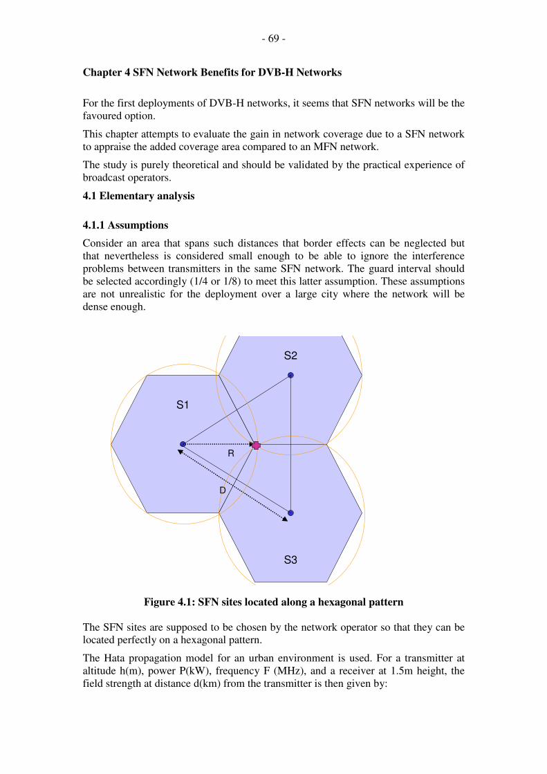
- 69 -

Chapter 4 SFN Network Benefits for DVB-H Networks

For the first deployments of DVB-H networks, it seems that SFN networks will be the

favoured option.

This chapter attempts to evaluate the gain in network coverage due to a SFN network

to appraise the added coverage area compared to an MFN network.

The study is purely theoretical and should be validated by the practical experience of

broadcast operators.

4.1 Elementary analysis

4.1.1 Assumptions

Consider an area that spans such distances that border effects can be neglected but

that nevertheless is considered small enough to be able to ignore the interference

problems between transmitters in the same SFN network. The guard interval should

be selected accordingly (1/4 or 1/8) to meet this latter assumption. These assumptions

are not unrealistic for the deployment over a large city where the network will be

dense enough.

S1

S2

S3

R

D

Figure 4.1: SFN sites located along a hexagonal pattern

The SFN sites are supposed to be chosen by the network operator so that they can be

located perfectly on a hexagonal pattern.

The Hata propagation model for an urban environment is used. For a transmitter at

altitude h(m), power P(kW), frequency F (MHz), and a receiver at 1.5m height, the

field strength at distance d(km) from the transmitter is then given by:

- 70 -

E(dBµV/m) = 10*log(P) - (44,9-6,55*log(h))*log(d) +K(F,h)

With K(F, h) = 67,65 –6,16*log(F) + 13,82*log(h)

Finally, all sites are considered to have the same height ho and the same transmission

power Po.

4.1.2 Derivation of the optimal distance

Considering the location A, indicated by red cross the on the above figure, the

combined field strength is the same as that of a single transmitter with ERP

P=Po+10*log(3), at a distance RSFN, since all three transmitters have the same

contribution.

In the case of a MFN, only one transmitter would have to create the field strength.

If the MFN transmitter covers an area with radius RMFN, the radius of SFN cells with

the same power is RSFN such that:

10*log(Po) - (44.9-6.55*log(h))*log(RSFN) = 10*log(Po) + 10*log(3) - (44.9-

6.55*log(h))*log(RMFN)

or

)hlog(55.69.44

)3log(10)

R

Rlog(

MFN

SFN

−=

The optimal distance between two sites can thus be derived:

MFN

)hlog(55.69.44

)3log(10

SFN R310D −=

Because the location A is the most difficult location to cover given this hexagonal

pattern, when the distance between sites is DSFN, the whole of the hexagon will be

covered and the coverage gain in surface area is:

2

MFN

2

SFN

SFNR

D2

3

aGainSurfaceAre⋅

=π

- 1

1102

33aGainSurfaceAre )hlog(55.69.44

)3log(20

SFN −⋅= −

π

Examples

Antenna Height 50m 200m

RSFN 1,38 RMFN 1,45 RMFN

- 71 -

DSFN 2,40 RMFN 2,50 RMFN

SurfaceAreaGainSFN 59% 73%

This means that in theory, the gain in surface area covered when using an SFN

can be quite large.

In the above computations, the assumption is made that the field strength of several

field strengths is the linear sum of these individual field strengths in µV/m. Because field strength is always a statistical variable, this is not entirely true. However, the use

of more accurate formulas will always yield more optimistic results. The gain in

surface area computed here is therefore a minimum gain.

Figure 4.2 illustrates the result of a simulation: three transmitters are located at equal

distances and would cover the blue area if they were on three different frequencies in

a MFN. The yellow area corresponds to the additional area covered by the SFN gain.

In Figure 4.2, the symmetry is not complete for the yellow area since the simulation is

only performed for transmitters radiating in one quarter of a plane only. Therefore,

only the triangle between the three sites is relevant here.

Figure 4.2: Illustration of SFN gain

Limitations

The above computations apply for an optimal site selection with the optimal distance.

In a real life situation, the distance will vary between transmitters.

Figure 4.3 shows using again the simulations for a transmitter at 1kW and site heights

of 50 m and 200m respectively that the SFN gain will vary quickly depending on the

selected distance between sites. Obviously, when SFN sites are located too close to

each other there is a loss in efficiency as there is overlap between the covered areas

rather than a constructive effect.

- 72 -

0,00%

10,00%

20,00%

30,00%

40,00%

50,00%

60,00%

0 2 4 6 8

Distance between transmitters (km)

Ga

in in

co

ve

red

s

urf

ac

e (

%)

50m

200m

Figure 4.3: Gain area coverage variations depending on distance between

transmitters

Figure 4.3 clearly shows that although the gain can be quite impressive (above 50%), it can also be limited (10%).

On the basis of this study only, it can therefore be considered dangerous to rely

on the gain in coverage due to the SFN network for real life network planning.

The next section will try to adopt a more rigorous approach as this preliminary study

does not enable clear conclusions to be drawn.

4.2 Simulation based analysis

4.2.1 Assumptions

The study is now uniquely based on the comparison between THREE transmission

sites in a SFN and the same sites in a MFN. The propagation model is still the

Okumura Hata model, at 1.5m, for urban planning.

The gain in surface area is computed as:

1Surface

3/ceTotalSurfaaGainSurfaceAre

Tx1_MFN

Tx3_SFN

SFN −=

The gain is estimated as the surface area covered by one site of a SFN using the SFN

contributions of other sites, divided by the surface are covered by one single site of a

MFN.

- 73 -

S1

S2

S3

R

D

Figure 4.4: Model with 3 transmitters

The simulation is run with a 100m computing step.

For every 100m x 100m square, the following algorithm is applied:

- compute the field strength created by each transmitter using the Okumura Hata model

- compute the mean (resultingMeanFieldStrength) and standard deviation

(resultingStdFieldStrength ) of the resulting field strengths using the tLNM method,

assuming that all field strengths have the same standard deviation

inputStdFieldStrength

- decide that the square is covered

in a SFN, when

resultingMeanFieldStrength >= RequiredMeanFieldStrength +

corFactor*resultingStdFieldStrength

in a MFN, when

resultingMeanFieldStrength >= RequiredMeanFieldStrength +

corFactor*inputStdFieldStrength

corFactor is the correction factor to cover 50% (0), 70% (0.55), 95% (1.65) or

99% (2.33) of the locations. It simply assumes a lognormal distribution of the field

strengths.

RequireMeanFieldStrength is the average field strength required to cover 50% of

the locations for a given transmission mode.

4.2.2 Results The simulation was run for two different configurations:

- 3 transmitters at 200m, 1kW ERP, for reception in mobility.

- 3 transmitters at 50m, 1kW ERP, for reception in mobility.

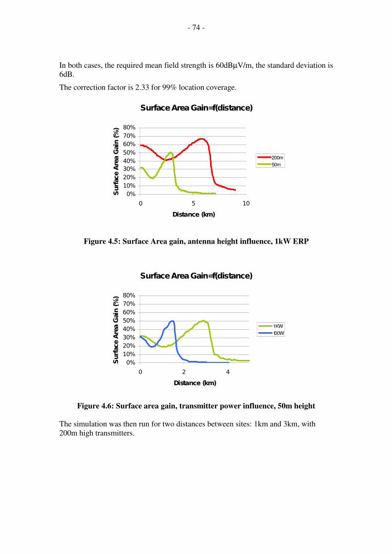
- 74 -

In both cases, the required mean field strength is 60dBµV/m, the standard deviation is 6dB.

The correction factor is 2.33 for 99% location coverage.

Surface Area Gain=f(distance)

0%

10%

20%

30%

40%

50%

60%

70%

80%

0 5 10

Distance (km)

Surface Area Gain (%)

200m

50m

Figure 4.5: Surface Area gain, antenna height influence, 1kW ERP

Surface Area Gain=f(distance)

0%

10%

20%

30%

40%

50%

60%

70%

80%

0 2 4

Distance (km)

Surface Area Gain (%)

1 KW

100W

Figure 4.6: Surface area gain, transmitter power influence, 50m height

The simulation was then run for two distances between sites: 1km and 3km, with

200m high transmitters.

- 75 -

Surface Area Gain =f(ERP)

30%

35%

40%

45%

50%

55%

60%

65%

70%

0 2000 4000 6000

ERP (W)

Su

rface A

rea G

ain

(%

)

1km

3km

Figure 4.7: Surface area gain, ERP influence for a given spacing of transmitters

Surface Area gain =f (Nb Sites)

0%

50%

100%

150%

200%

250%

0 10 20 30 40 50 60

Nb Sites

% o

f su

rface a

rea c

overe

d

Figure 4.8: Surface area gain, influence of number of sites

In Figure 4.9, the transmitters are spaced at a quasi-optimal distance, for the 200m

height case. The area in green corresponds to the coverage of the MFN, the area in

blue is the additional area covered by the SFN.

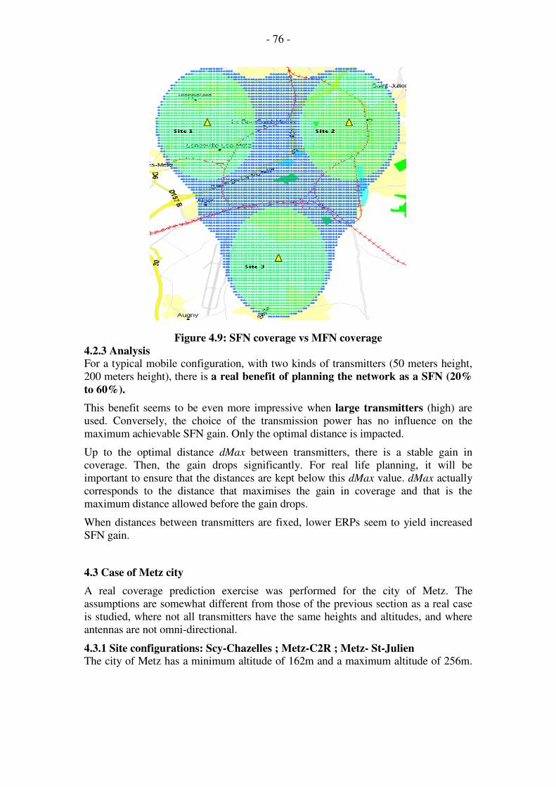
- 76 -

Figure 4.9: SFN coverage vs MFN coverage

4.2.3 Analysis

For a typical mobile configuration, with two kinds of transmitters (50 meters height,

200 meters height), there is a real benefit of planning the network as a SFN (20%

to 60%).

This benefit seems to be even more impressive when large transmitters (high) are

used. Conversely, the choice of the transmission power has no influence on the

maximum achievable SFN gain. Only the optimal distance is impacted.

Up to the optimal distance dMax between transmitters, there is a stable gain in

coverage. Then, the gain drops significantly. For real life planning, it will be

important to ensure that the distances are kept below this dMax value. dMax actually

corresponds to the distance that maximises the gain in coverage and that is the

maximum distance allowed before the gain drops.

When distances between transmitters are fixed, lower ERPs seem to yield increased

SFN gain.

4.3 Case of Metz city

A real coverage prediction exercise was performed for the city of Metz. The

assumptions are somewhat different from those of the previous section as a real case

is studied, where not all transmitters have the same heights and altitudes, and where

antennas are not omni-directional.

4.3.1 Site configurations: Scy-Chazelles ; Metz-C2R ; Metz- St-Julien

The city of Metz has a minimum altitude of 162m and a maximum altitude of 256m.

- 77 -

Transmitters Transmission

height

Polarisation Frequency ERP Azimut Radiation pattern (horizontal

and vertical)

Scy-Chazelles 30 m Vertical 706 MHz

(C50) 600/1200 W

110 °

Metz-C2R 45 m Vertical 706 MHz

(C50)

600/ 1200

W

290 °

Metz- St-

Julien 60 m Vertical

706 MHz

(C50)

600/ 1200

W

230 °

Table 4.1: Site transmission specifications

Site Code

IG

Latitude Longitude Altitude Estimated

effective

height

Distance to

C2R

Scy-Chazelles - Fort

Diou

576420

3

49°07’17’’N 06°07’48’’E 353 m 221 m 6.4km

Metz-C2R 574630

1

49°06’12’’N 06°12’53’’E 200 m 83 m 0km

Metz- St-Julien 576160

1

49°08’30’’N 06°13’00’’E 262 m 160 m 4.26km

Table 4.2: Site coordinates and effective heights

4.3.2 Required Field strength

Two cases are studied: QPSK ½ for which it is estimated that 79dBuV/m is necessary,

and 16QAM ½ for which it is estimated that 85 dBuV/m is required.

- 78 -

4.3.3 Results

Figure 4.10: Comparison of MFN and SFN coverage, QPSK 1/2, 1200W ERP

Covered area (km²)

QPSK 1/2 16QAM ½

Transmitter 600 W 1200 W 600 W 1200 W

Scy-Chazelles 6.06 11.91 1.57 4.04

Metz-C2R 1.98 4.03 0.76 1.21

Metz-St-Julien 7.20 14.71 1.53 3.69

Three sites 14.30 25.84 3.85 8.94

Service zones 24.38 41.90 6.91 13.38

SFN gain 60% 37% 79% 50%

Table 4.3: Covered areas in each configuration, SFN gain

- 79 -

The SFN gain is computed as the ratio of the service zone divided by the sum of all

three individual surface areas (Scy-Chazelles, Metz-C2R, Metz-St-Julien), according

to the definition used in section 2.

The results are similar or even better than those presented in section 3: the SFN gain

is quite noticeable, with values of 60% gain easily reached.

It is also interesting to notice the same trend seen in section 3: for a given distance

between transmitters, the SFN gain increases when the ERP of the transmitters

decreases.

4.4 Conclusions

SFN gain can be substantial: from 20% in a worst case scenario, to 70% in the case

of optimised site location, ERP and heights, for three transmitters.

SFN gain is even larger when small sites are deployed: little ERP on a large

number of sites will increase the SFN gain.

Although the SFN gain can be quite impressive in the case of a large number of

sites, with values over 100% in the case of 10+ sites, the cost of deployment must be

taken into account, and it is anticipated that the cost of the site multiplication will

not be compensated for by the SFN gain.

- 80 -

Chapter 5 Study of SFN for DVB-H networks

The objective of this chapter is to determine, at a broadcast operator investment cost

level, what is the best configuration for a DVB-H SFN network deployment. Would it

be more interesting to use large or small sites? Results of simulations (made with the

TDF proprietary radio planning tool), for several configurations, and with working

assumptions close to future deployments, are presented.

5.1 Assumptions

5.1.1 DVB specifications

Modulation QPSK

Code rate ½

Guard interval 1/8

Mode 8 k

Net bit rate (Mbits/s) 5,53

Table 5.1: DVB specifications

5.1.2 Transmission • The transmission will be achieved on channel 50 (706 MHz)

5.1.3 Reception

Some assumptions are made concerning the specifications of DVB-H receivers:

• Handheld portable convergence terminals are considered

• The terminals are used according to the four user classes defined in the ETSI guidelines:

Class A Portable outdoor

Class B Portable indoor

Class C Mobile outdoor

Class D Inside mobile

Table 5.2: Classes

• Only the worst reception case, class D, will be considered

Note: In the "inside mobile" reception situation, no external antennas are used.

• Receiver antenna: patch antenna (Nokia 7700)

• Reception height is 1.50 m

• Vertical polarisation

• Noise factor = 6 dB

• Penetration margin (in car) = 8 dB

• Dense urban environment (DU)

- 81 -

• The standard deviation of the signal inside the vehicle is taken equal to 6 dB, in

spite of the recommendations advocating a standard deviation of 5.5 dB, for reception

with a rooftop antenna. For indoor portability, the advised standard deviation is 8.1

dB. In a configuration of a terminal with an integrated antenna, inside a vehicle, the

environment is a priori less restrictive than indoor portability, but more restrictive

than rooftop reception, therefore 6 dB is chosen.

• MPE-FEC is not taken into account

The synchronisation strategy is the one of the Nokia 7700 receiver (cf. graph below).

5.1.4 Field strength

The formula used, comes from the Chester agreement:

E = F + 10log(KTB) + C/N – Gr – 10log(1.64 * (c/f)^2 / (4*π) ) + p + 145.8 + σ * correction + penetration

The propagation model is the TDF "digital TV portability" model version 2.0,

calibrated for a reception height of 2 meters, in an urban area, UHF band, and for

distances lower than 20 km.

Delay (µs)

C/I (dB)

- 82 -

QPSK ½

Class D

Boltzmann constant K 1.38.10-23

Temperature T (K) 290

Bandwidth B (Hz) 7.61.106

Noise factor F (dB) 6

C/N (dB) 9.5

Reception antenna gain Gr (dBd) -15

Frequency f (MHz) 706 (C50)

Losses p (dB) 0

Minimum median equivalent field

strength at 1.5 m, 50 % of locations

(dBµV/m)

57.41

Standard deviation σσσσ (dB) 6

Percentage of locations (%)

99

(correction

coefficient

= 2.33)

Penetration losses (dB) 8

Minimum median equivalent field

strength at 1.5 m, x% of locations

(dBµV/m)

79.39

Table 5.3: Minimum median equivalent field strength at 1.5 m for class D –

QPSK modulation

Consequently, the tested field level will be 80 dBµV/m, for the QPSK modulation.

5.1.5 Configurations Thanks to a TDF cost function, based on CAPEX, a calculation has enabled it to be

determined that the following configurations lead to similar investment costs:

- HTx = 150 m, ERP = 5 kW, 3 sites,

- HTx = 75 m, ERP = 400 W, 10 sites,

- HTx = 50 m, ERP = 100 W, 15 sites.

Consequently, simulations will be made of these three configurations, to determine

the best configuration in a dense urban environment.

- 83 -

5.2 Prediction coverages

5.2.1 Site configurations

5.2.1.1 Specifications

The geographical coordinates of the sites (coordinates, altitude), in each

configuration, are given in Appendix 5.

5.2.1.2 Transmission specifications

Transmitters Transmission

height

Polarisation Frequency ERP Radiation pattern (horizontal

and vertical)

Site C1 150 m Vertical 706 MHz

(C50) 5 000 W


(C50) 400 W


(C50) 100 W

Table 5.4: Site transmission specifications in each configuration (C1, C2, C3)

5.2.2 Simulation parameters

• Atoll version 2.1.0 is the radio network planning tool, associated with Ivoire 1.7.1

(TDF).

• The propagation model is the TDF "digital TV portability" model version 2.0,

calibrated for a 2-meter high reception, in an urban area, UHF band, and for distances

lower than 20 km.

• The terrain database is the DEM (Digital Elevation Model) of Paris, with a 4m

resolution,

• The calculation step is 25 meters for prediction coverage, and 50 m for service

zones (a trade-off between accuracy and processing time),

Note:

1. The portability model is a semi statistical model calibrated for a height of 2 meters

(real reception height is 1.5 m, so the attenuation due to the height difference (0.5 m)

is considered negligible). It is valid only in the vertical plan (diffracting edge profile),

and hence, does not take into account the multiple reflections in the horizontal plan,

that is characteristic of propagation in an urban area. Only terrain measurements can

corroborate the predictions presented here.

- 84 -

2. The predicted coverages presented take into account the potential interferences

caused by the other transmitters.

5.2.3 Configuration 1: HTx = 150 m, ERP = 5 kW, 3 sites

The distance between two sites is 6 kms.

Figure 5.1: Service zone for configuration 1

Scale: 1 cm ↔↔↔↔ 1.72 km

Note:

1. The red frame represents the working zone.

2. The coordinates (NTF France II extended) of the reference point (Louvre

Pyramid), on the map zoomed in, are the following:

=

=

2429184

599952

y

x

80 dBµV/m

Road

- 85 -

Figure 5.2: Zoom on the service zone obtained for configuration

Scale: 1 cm ↔↔↔↔ 1.07 km

The Paris city centre (CC), limited by the ring road, is rather well covered for the field

level 80 dBµV/m. Significant holes of coverage (several hundreds of meters) are

visible in the north, and in the west. The coverage of the ring road is nearly

continuous.

5.2.4 Configuration 2: HTx = 75 m, ERP = 400 W, 10 sites

The distance between two sites is 1 km.


Scale: 1 cm ↔↔↔↔ 1.72 km

80 dBµV/m

Road

80 dBµV/m

Ring road

Reference point

- 86 -

Figure 5.4: Zoom on the service zone obtained for configuration 2

Scale: 1 cm ↔↔↔↔ 1.07 km

The coverage of the CC is distinctly reduced (46 km²), in comparison with the first

configuration. A big part of the city centre is no longer covered, and the ring road

does not have any coverage.

5.2.5 Configuration 3: HTx = 50 m, ERP = 100 W, 15 sites

The distance between two sites is 400 m.

80 dBµV/m

Ring road

- 87 -


Scale: 1 cm ↔↔↔↔ 1.72 km

Figure 5.6: Zoom on the service zone obtained for configuration 2

Scale: 1 cm ↔↔↔↔ 1.07 km

The coverage is much smaller (12 km²) than the two previous ones.

80 dBµV/m

Road

- 88 -

5.3 Synthesis

5.3.1 Covered areas

Table 5.5 lists the covered areas obtained for each configuration. The coverage

predictions are limited by the working zone defined under Atoll (surface = 266 km²)

Modulation Signal level

(dBµµµµV/m)

Transmitter Covered area (km²)

Configuration 1 195

Configuration 2 46

QPSK 80

Configuration 3 12

Table 5.5: Covered areas in each configuration

CC: City centre

5.4 Conclusions

First, it is important to emphasise that the reception case considered in this chapter is

the worst one: the class D (inside mobility), and the terminal used for the simulations

is the mobile Nokia 7700. It must be noted that the propagation model used, does not

take into account the propagation into the horizontal plane.

The city centre of Paris is well covered within the first configuration: 150 m high, 5

kW ERP, and three sites. In the second configuration the global coverage decreases

distinctly, and finally, for the third configuration the coverage is drastically reduced.

The simulations presented in this chapter clearly show that large sites give the

best coverage, for a SFN DVB-H QPSK ½ 8k 1/8 class D case, in a dense urban

environment (centre of Paris).

The SFN gain can be quite important in the case of a large number of sites. However,

it is shown here, that the cost of the site multiplication is not compensated for by

the SFN gain.

Bad coverage in the CC

Medium coverage in the CC

Good coverage in the CC

- 89 -

Chapter 6 DVB-H, GSM900, GSM1800 and UMTS cositing analysis

6.1 Introduction

This chapter presents cositing issues between the DVB-H system and radiocom

services (GSM900, GSM1800, and UMTS). The main topic is Electro-Magnetic

Compatibility (EMC) between radio systems. In the first part of this chapter the

isolation required between systems, to maintain an acceptable Quality of Service

(QoS), is derived from radio equipment specifications, and in the second part of the

chapter possible cositing architectures are proposed in terms of antenna spacing.

For the EMC analysis three types of interferers are taken into account:

- Spurious emissions from one transmitter falling into the receive band of a

cosited receiver

- The blocking effect, that may occur when a strong interferer is located nearby

a receiver

- The intermodulation products that are generated when several transmitters are

cosited

6.1.1 Frequency bands of studied systems

Uplink (UL)

Mobile →→→→ Basestation

Downlink (DL)

Basestation →→→→ Mobile

GSM900 880 – 915 MHz 925 – 960 MHz

GSM1800 1710 – 1785 MHz 1805 – 1880 MHz

WCDMA - FDD 1920 – 1980 MHz 2110 – 2170 MHz

DVB-H Not applicable 470 – 860 MHz

Table 6.1: Frequency bands of studied systems

6.1.2 Decoupling between antennas

The decoupling values between antennas will be evaluated thanks to the software tool

named Lorraine (TDF internal tool). The decoupling between antennas is considered

from antenna port to antenna port whereas the required isolation between systems is

considered from base-station connector to base-station connector.

Station1 Station 2

X dB

Figure 6.11: Decoupling between antennas

- 90 -

6.1.3 Spurious emissions

Spurious emissions from a transmitter are emissions outside the frequency band of the

useful signal. Spurious emissions falling into the receive frequency band of another

system may degrade its sensitivity. The specifications [1], [2], and [3] define the

maximum authorised level of spurious emissions for each system.

decouplingSystem 1 System 2

Spurious in the receive bandof system 2

Band 1 DL Band 2 UL

6.1.4 Inter-modulation products

When two or more transmitters coexist on a site interfering frequencies may occur

resulting from the mixing of several useful signals. If these intermodulation products

fall into the receive band of a receiver, they may degrade its sensitivity.

decouplingSys. 1 Sys. 2

F2-F1 2xF2-F1

F1 F2

The level of intermodulation products shall not be higher than the maximum level of

spurious emission as indicated in the specifications [1], [2], and [3].

6.1.5 Sensitivity degradation

This subsection describes the computation of the sensitivity degradation of a receiver

in the presence of interferer.

The expressions for the sensitivity of GSM900, GSM1800, UMTS and DVB-H

systems are:

GSM900 Sensitivity [dBm] = GSM900 Noise Floor [dBm] + C/I [dB]

GSM1800 Sensitivity [dBm] = GSM1800 Noise Floor [dBm] + C/I [dB]

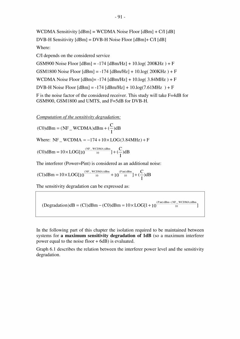
- 91 -

WCDMA Sensitivity [dBm] = WCDMA Noise Floor [dBm] + C/I [dB]

DVB-H Sensitivity [dBm] = DVB-H Noise Floor [dBm]+ C/I [dB]

Where:

C/I depends on the considered service

GSM900 Noise Floor [dBm] = -174 [dBm/Hz] + 10.log( 200KHz ) + F

GSM1800 Noise Floor [dBm] = -174 [dBm/Hz] + 10.log( 200KHz ) + F

WCDMA Noise Floor [dBm]= -174 [dBm/Hz] + 10.log( 3.84MHz ) + F

DVB-H Noise Floor [dBm] = -174 [dBm/Hz] + 10.log(7.61MHz ) + F

F is the noise factor of the considered receiver. This study will take F=4dB for

GSM900, GSM1800 and UMTS, and F=5dB for DVB-H.

Computation of the sensitivity degradation:

dB)I

C(dBm)WCDMA_NF(dBm)0C( +=

Where: F)MHz84.3(LOG10174WCDMA_NF +×+−=

dB)I

C(]10[LOG10dBm)0C( 10

dBm)WCDMA_NF(

+×=

The interferer (Power=Pint) is considered as an additional noise:

dB)I

C(]1010[LOG10dBm)1C( 10

dBmint)P(

10

dBm)WCDMA_NF(

++×=

The sensitivity degradation can be expressed as:

]101[LOG10dBm)0C(dBm)1C(dB)nDegradatio( 10

dBm)WCDMA_NF(dBmint)P( −

+×=−=

In the following part of this chapter the isolation required to be maintained between

systems for a maximum sensitivity degradation of 1dB (so a maximum interferer

power equal to the noise floor + 6dB) is evaluated.

Graph 6.1 describes the relation between the interferer power level and the sensitivity

degradation.

- 92 -

Pint/NF (dB)

-16,3

-13,3

-11,5

-10,2-9,1

-8,3-7,6

-6,9-6,4 -5,9

-18,0

-16,0

-14,0

-12,0

-10,0

-8,0

-6,0

-4,0

-2,0

0,0

0 0,2 0,4 0,6 0,8 1

Sensitivity degradation(dB)

Graph 6.1: Sensitivity degradation versus interferer power

6.1.6 Blocking

The blocking risk that may occur when a strong signal is located nearby a receiver

will be taken into account.

A maximum sensitivity degradation of 1dB due to the blocking effect will be

considered.

decouplingSystem 1 System 2

Selectivity filter of receiver 2

Band 1 DL Band 2 UL

Selectivity at f1

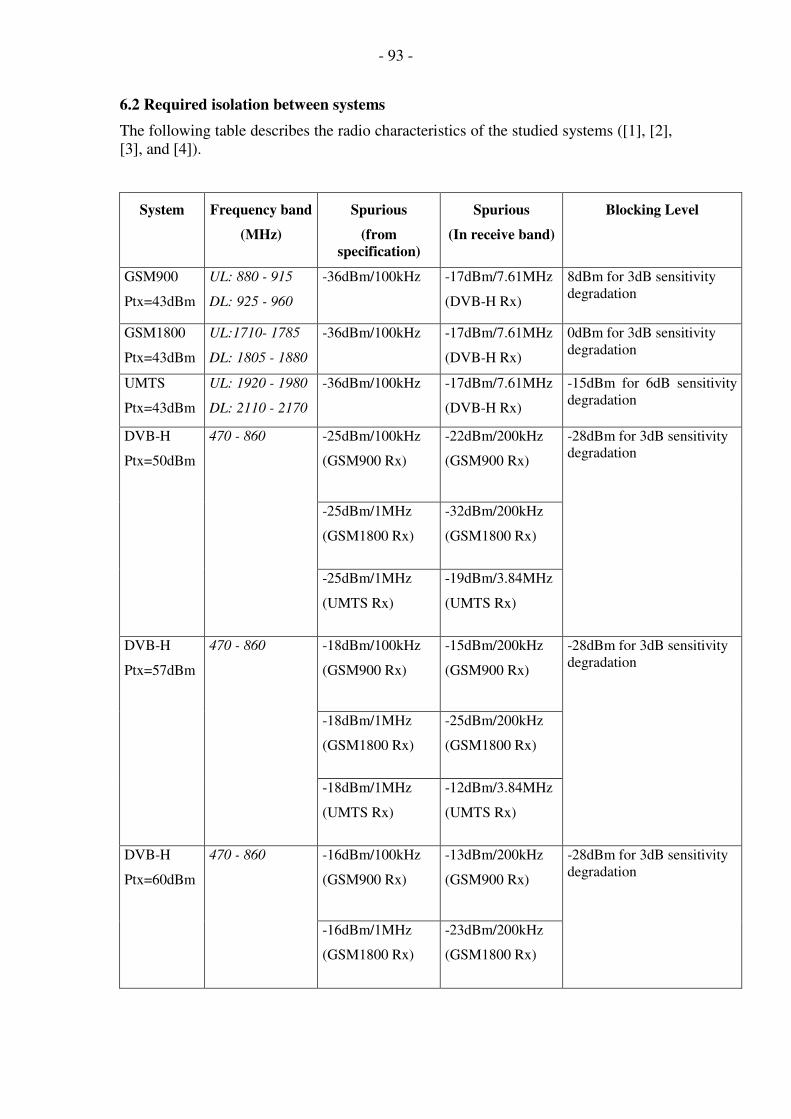
- 93 -

6.2 Required isolation between systems

The following table describes the radio characteristics of the studied systems ([1], [2],

[3], and [4]).

System Frequency band

(MHz)

Spurious

(from

specification)

Spurious

(In receive band)

Blocking Level

GSM900

Ptx=43dBm

UL: 880 - 915

DL: 925 - 960

-36dBm/100kHz -17dBm/7.61MHz

(DVB-H Rx)

8dBm for 3dB sensitivity

degradation

GSM1800

Ptx=43dBm

UL:1710- 1785

DL: 1805 - 1880


(DVB-H Rx)

0dBm for 3dB sensitivity

degradation

UMTS

Ptx=43dBm

UL: 1920 - 1980

DL: 2110 - 2170


(DVB-H Rx)

-15dBm for 6dB sensitivity

degradation

-25dBm/100kHz

(GSM900 Rx)

-22dBm/200kHz

(GSM900 Rx)

-25dBm/1MHz

(GSM1800 Rx)

-32dBm/200kHz

(GSM1800 Rx)

DVB-H

Ptx=50dBm

470 - 860

-25dBm/1MHz

(UMTS Rx)

-19dBm/3.84MHz

(UMTS Rx)


degradation

-18dBm/100kHz

(GSM900 Rx)

-15dBm/200kHz

(GSM900 Rx)

-18dBm/1MHz

(GSM1800 Rx)

-25dBm/200kHz

(GSM1800 Rx)

DVB-H

Ptx=57dBm

470 - 860

-18dBm/1MHz

(UMTS Rx)

-12dBm/3.84MHz

(UMTS Rx)


degradation

-16dBm/100kHz

(GSM900 Rx)

-13dBm/200kHz

(GSM900 Rx)

DVB-H

Ptx=60dBm

470 - 860

-16dBm/1MHz

(GSM1800 Rx)

-23dBm/200kHz

(GSM1800 Rx)


degradation

- 94 -

-16dBm/1MHz

(UMTS Rx)

-10dBm/3.84MHz

(UMTS Rx)

Table 6.2: Radio characteristics

Table 6.3 gives the required isolation values to ensure a maximum sensitivity

degradation of 1dB for the DVB-H receiver.

1

Victim

Aggressor DVB-H

A GSM 900

Pem = +43dBm

Spurious : 89dB(Case n° 1:)

Blocking : 77dB(Case n° 5)

B GSM 1800

Pem = +43dBm



C UMTS

Pem = +43dBm



Table 6.3: Required isolation to protect the DVB-H receiver

Table 6.4 gives the required isolation values to ensure a maximum sensitivity

degradation of 1dB for the radiocom receivers.

1 2 3

GSM 900 GSM 1800 UMTS

D DVB-H

Pem = +50dBm

Spurious : 101dB(

Case n° 2)

Blocking : 48dB

(Case n° 6)

Spurious : 91dB(Case

n° 3:)

Blocking : 56dB

(Case n°7)


n° 4:)

Blocking : 76dB

(Case n° 8)

E DVB-H

Pem = +57dBm


n°9:)

Blocking : 55dB

(Case n°15)


n°10)

Blocking : 63dB

(Case n°16)


n°11)

Blocking : 83dB

(Case n°17)

F DVB-H

Pem = +60dBm


n°12)

Blocking : 58dB

(Case n°18)


n°13)

Blocking : 66dB

(Case n°19)


n°14)

Blocking : 86dB

(Case n°20)

Table 6.4: Required isolation to protect the radiocom receivers

Victim

Aggressor

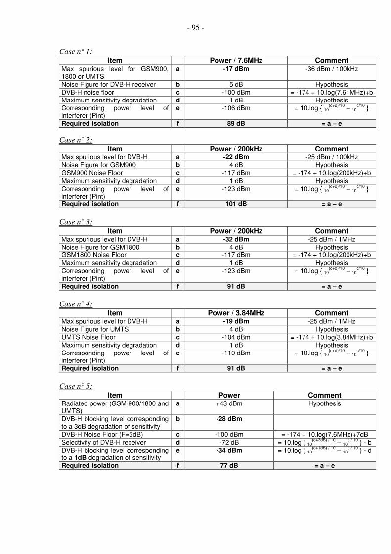
- 95 -

Case n° 1:

Item Power / 7.6MHz Comment Max spurious level for GSM900, 1800 or UMTS

a -17 dBm -36 dBm / 100kHz

Noise Figure for DVB-H receiver b 5 dB Hypothesis DVB-H noise floor c -100 dBm = -174 + 10.log(7.61MHz)+b Maximum sensitivity degradation d 1 dB Hypothesis Corresponding power level of interferer (Pint)

e -106 dBm = 10.log 10(c+d)/10

– 10c/10

Required isolation f 89 dB = a – e

Case n° 2:

Item Power / 200kHz Comment Max spurious level for DVB-H a -22 dBm -25 dBm / 100kHz Noise Figure for GSM900 b 4 dB Hypothesis GSM900 Noise Floor c -117 dBm = -174 + 10.log(200kHz)+b Maximum sensitivity degradation d 1 dB Hypothesis Corresponding power level of interferer (Pint)

e -123 dBm = 10.log 10(c+d)/10

– 10c/10


Case n° 3:

Item Power / 200kHz Comment Max spurious level for DVB-H a -32 dBm -25 dBm / 1MHz Noise Figure for GSM1800 b 4 dB Hypothesis GSM1800 Noise Floor c -117 dBm = -174 + 10.log(200kHz)+b Maximum sensitivity degradation d 1 dB Hypothesis Corresponding power level of interferer (Pint)

e -123 dBm = 10.log 10(c+d)/10

– 10c/10


Case n° 4:

Item Power / 3.84MHz Comment Max spurious level for DVB-H a -19 dBm -25 dBm / 1MHz

Noise Figure for UMTS b 4 dB Hypothesis UMTS Noise Floor c -104 dBm = -174 + 10.log(3.84MHz)+b Maximum sensitivity degradation d 1 dB Hypothesis Corresponding power level of interferer (Pint)

e -110 dBm = 10.log 10(c+d)/10

– 10c/10


Case n° 5:

Item Power Comment Radiated power (GSM 900/1800 and UMTS)

a +43 dBm Hypothesis

DVB-H blocking level corresponding to a 3dB degradation of sensitivity

b -28 dBm

DVB-H Noise Floor (F=5dB) c -100 dBm = -174 + 10.log(7.6MHz)+7dB Selectivity of DVB-H receiver d -72 dB = 10.log 10

(c+3dB) / 10 – 10

c / 10 - b

DVB-H blocking level corresponding to a 1dB degradation of sensitivity

e -34 dBm = 10.log 10(c+1dB) / 10

– 10c / 10

- d


- 96 -

Case n° 6:

Item Power Comment Radiated power (DVB-H) a +50 dBm Hypothesis GSM900 blocking level corresponding to a 3dB degradation of sensitivity

b 8 dBm GSM 05.05 specification

GSM900 Noise Floor (F=4dB) c -117 dBm = -174 + 10.log(200KHz)+4dB Selectivity of GSM900 receiver d -125 dB = 10.log 10

(c+3dB) / 10 – 10

c / 10 - b

GSM900 blocking level corresponding to a 1dB degradation of sensitivity

e +2 dBm = 10.log 10(c+1dB) / 10

– 10c / 10

- d


Case n°7:




(c+3dB) / 10 – 10

c / 10 - b


e -6 dBm = 10.log 10(c+1dB) / 10

– 10c / 10

- d


Case n° 8:

Item Power Comment Radiated power (DVB-H) a +50 dBm Hypothesis UMTS blocking level corresponding to a 6dB degradation of sensitivity

b -15 dBm

UMTS Noise Floor (F=4dB) c -104 dBm = -174 + 10.log(3.84MHz)+4dB Selectivity of UMTS receiver d -84 dB = 10.log 10

(c+6dB) / 10 – 10

c / 10 - b

UMTS blocking level corresponding to a 1dB degradation of sensitivity

e -26 dBm = 10.log 10(c+1dB) / 10

– 10c / 10

- d


Case n°9:


e -123 dBm = 10.log 10(c+d)/10

– 10c/10


Case n°10:


e -123 dBm = 10.log 10(c+d)/10

– 10c/10


- 97 -

Case n°11:



e -110 dBm = 10.log 10(c+d)/10

– 10c/10


Case n°12:


e -123 dBm = 10.log 10(c+d)/10

– 10c/10


Case n°13:


e -123 dBm = 10.log 10(c+d)/10

– 10c/10


Case n°14:



e -110 dBm = 10.log 10(c+d)/10

– 10c/10


Case n°15:




(c+3dB) / 10 – 10

c / 10 - b


e +2 dBm = 10.log 10(c+1dB) / 10

– 10c / 10

- d


- 98 -

Case n°16:




(c+3dB) / 10 – 10

c / 10 - b


e -6 dBm = 10.log 10(c+1dB) / 10

– 10c / 10

- d


Case n°17:


b -15 dBm

UMTS Noise Floor (F=4dB) c -104 dBm = -174 + 10.log(3.84MHz)+4dB Selectivity of UMTS receiver d -84 dB = 10.log 10

(c+6dB) / 10 – 10

c / 10 - b

UMTS blocking level corresponding to a 1dB degradation of sensitivity

e -26 dBm = 10.log 10(c+1dB) / 10

– 10c / 10

- d


Case n°18:




(c+3dB) / 10 – 10

c / 10 - b


e +2 dBm = 10.log 10(c+1dB) / 10

– 10c / 10

- d


Case n°19:




(c+3dB) / 10 – 10

c / 10 - b


e -6 dBm = 10.log 10(c+1dB) / 10

– 10c / 10

- d


Case n°20:


b -15 dBm

UMTS Noise Floor (F=4dB) c -104 dBm = -174 + 10.log(3.84MHz)+4dB

- 99 -

Selectivity of UMTS receiver d -84 dB = 10.log 10(c+6dB) / 10

– 10c / 10

- b UMTS blocking level corresponding to a 1dB degradation of sensitivity

e -26 dBm = 10.log 10(c+1dB) / 10

– 10c / 10

- d


6.3 DVB-H and radiocom services cositing architectures

6.3.1 General points

DVB-H sites:

Two kinds of DVB-H sites are considered in this study: the transmitter only site and

the repeater site where both receiver and re-transmitter coexist. In the latter case

enough isolation must be provided between the receiver and the transmitter for the

system to work properly (10-15 dB above the re-transmitter gain).

DVB-H sites are high power sites, compared to radiocom sites. DVB-H transmitter

power ranges from 100W to 1kW. Considered transmitting antennas consist of several

UHF panel antennas, with an equivalent omni-directional pattern. The considered

antenna gain is 10 dBi, and the vertical 3dB aperture is 30°.

In repeater sites, the DVB-H receiver antenna is a log-periodic one, located below the

transmitter antennas.

Radiocom sites:

Radiocom sites are mostly tri-sector sites. Base station transmitter power is 20W.

Radiocom antennas are directional panel antennas with 65° horizontal aperture, 7°

vertical aperture, and 17dBi gain.

DVB-H + Radiocoms cositing architecture:

Figure 6.12: DVB-H and radiocom cositing architecture

Array of UHF

panel antennas

Radiocom panel

antennas

UHF Log-

periodoic antenna

DVB-H Tx

Radiocom

Tx/Rx

DVB-H Rx

? m

? m

- 100 -

In the following subsections, decoupling calculations will be performed and minimum

separation distances will be proposed for such cositing architectures.

6.3.2 DVB-H and GSM900

6.3.2.1 Input data

Figure 6.13: Diagram of GSM900-DVBT site

It is assumed that:

• feeders + jumpers losses = 3 dB

• Panel antenna, ±45° dual polarisation, 3dB aperture of 65° (horizontal plane), 3dB aperture of 7° (vertical plane), 17 dBi gain, for GSM

• Array of panel antennas, vertically polarised, 3dB aperture of 30° (vertical plane), 10 dBi gain, for DVB-H Tx

• Log-periodic antenna, horizontally polarised, 3dB aperture of 50° (horizontal

plane), 3dB aperture of 60° (vertical plane), 10.5 dBi gain, for DVB-H Rx in case

of repeater site.

6.3.2.2 Theoretical decoupling between antennas

The simulations are carried out for the antenna arrangement described in Figure 6.14

and Figure 6.15. Graph 6.2 and Graph 6.3 show the attenuation between the two

antennas versus the inter-antenna distance (d) at different frequencies.

I

I

I I

DVB-H

Tx Rx

(if

applicable)

X

X

X

X

GSM

900

Tx/Rx Rx

diversity

- 101 -

d

DVB-H

Tx

GSM900

Figure 6.14: GSM900 / DVB-H Tx antenna arrangement

60

65

70

75

80

85

90

95

100

0 5 10

d (m)

Deco

up

lin

g (

dB

)

600MHz

900MHz

Graph 6.2 : Vertical decoupling between GSM900 and DVB-H Tx antennas

d

GSM900

DVB-H Rx

Figure 6.15: GSM900 / DVB-H Rx antenna arrangement

- 102 -

60

70

80

90

100

110

0 2 4 6

d (m)

Deco

up

lin

g (

dB

)

600MHz

900MHz

Graph 6.3: Vertical decoupling between GSM900 and DVB-H Rx antennas

6.3.2.3 Required spacing between antennas

DVB-H Tx and GSM900:

DVB-H Tx power Minimum distance due to

DVB-H spurious

(Attenuation at 900MHz)

Minimum distance due to

GSM900 blocking


100W 10m + 6dB filter 2m


1kW 10m + 15dB filter 2m

Table 6.5: Minimum distance between DVB-H Tx and GSM 900 antennas

DVB-H Rx and GSM900:


GSM900 spurious (Attenuation at

600MHz)

Minimum distance due to DVB-

H blocking (Attenuation at

900MHz)

3m 1m

Table 6.6 : Minimum distance between DVB-H Rx and GSM 900 antennas

6.3.2.4 Proposed configuration

With a spacing of 10m between the DVB-H Tx and GSM900 antenna and a spacing

of 3m between the DVB-H Rx and GSM900 antenna, an additional bandpass filter is

needed on the DVB Tx port.

- 103 -

3m

GSM900

DVB-H Rx

10m

DVB-H Tx

6.3.3 DVB-H and GSM1800

6.3.3.1 Input data

Figure 6.16: Diagram of GSM1800-DVBH site

It is assumed that:


• Panel antenna, ±45° dual polarisation, 3dB aperture of 65° (horizontal plane), 3dB

aperture of 7° (vertical plane), 17 dBi gain, for GSM


I

I

I

I

DVB-H

Tx Rx

(if

applicable)

X

X

X

X

GSM

1800

Tx/Rx Rx

diversity

- 104 -

• Log-periodic antenna, horizontally polarised, 3dB aperture of 50° (horizontal plane), 3dB aperture of 60° (vertical plane), 10.5 dBi gain, for DVB-H Rx in the

case of a repeater site.


Simulations were carried out for the antenna arrangement described in Figure 6.17

and Figure 6.18. Graph 6.4 and Graph 6.5 show the attenuation between the two


d

DVB-H

Tx

GSM1800

Figure 6.17: GSM1800 / DVB-H Tx antenna arrangement

70

75

8085

9095

100

105

110

115

2 4 6 8 10

d (m)

Déco

up

lag

e (

dB

)

600MHz

1800MHz

Graph 6.4: Vertical decoupling between GSM1800 and DVB-H Tx antennas

- 105 -

d

GSM1800

DVB-H Rx

Figure 6.18: GSM1800 / DVB-H Rx antenna arrangement

70

75

80

85

90

95

100

105

110

0 1 2 3

d (m)

Déco

up

lag

e (

dB

)

600MHz

1800MHz

Graph 6.5: Vertical decoupling between GSM1800 and DVB-H Rx antennas


DVB-H Tx and GSM1800:


DVB-H spurious

(Attenuation at

1800MHz)


GSM1800 blocking


100W 6m 2m


1kW 6m + 9dB filter 2m

Table 6.7: Minimum distance between DVB-H Tx and GSM 1800 antennas

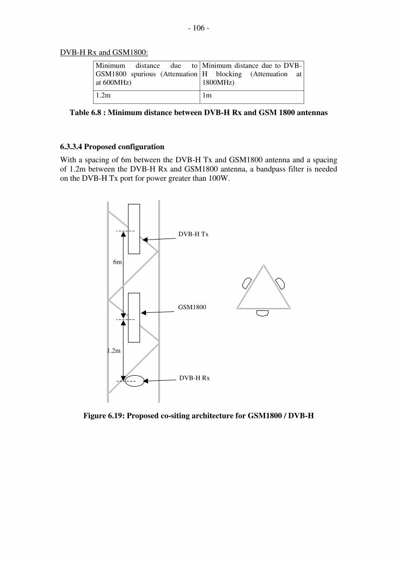
- 106 -

DVB-H Rx and GSM1800:


GSM1800 spurious (Attenuation

at 600MHz)



1800MHz)

1.2m 1m

Table 6.8 : Minimum distance between DVB-H Rx and GSM 1800 antennas


With a spacing of 6m between the DVB-H Tx and GSM1800 antenna and a spacing

of 1.2m between the DVB-H Rx and GSM1800 antenna, a bandpass filter is needed

on the DVB-H Tx port for power greater than 100W.

1.2m

GSM1800

DVB-H Rx

6m

DVB-H Tx

Figure 6.19: Proposed co-siting architecture for GSM1800 / DVB-H

- 107 -

6.3.4 DVB-H and UMTS

6.3.4.1 Input data

Figure 6.20: Diagram of UMTS/DVB-H site

It is assumed that:


• Panel antenna, ±45° dual polarisation, 3dB aperture of 65° (horizontal plane), 3dB

aperture of 7° (vertical plane), 17 dBi gain, for UMTS


• Log-periodic antenna, horizontally polarised, 3dB aperture of 50° (horizontal plane), 3dB aperture of 60° (vertical plane), 10.5 dBi gain, for DVB-H Rx in the

case of a repeater site.


The simulations were carried out for the antenna arrangement described in Figure

6.21 and Figure 6.22. Graph 6.6 and Graph 6.7 show the attenuation between the two


I

I

I I

DVB-H

Tx Rx

(if

applicable)

X

X

X

X

UMT

S

Tx/Rx Rx

diversity

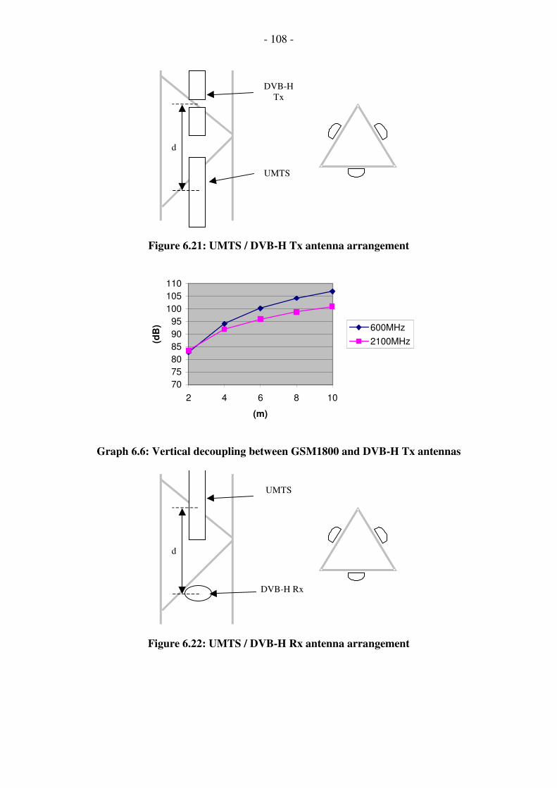
- 108 -

d

DVB-H

Tx

UMTS

Figure 6.21: UMTS / DVB-H Tx antenna arrangement

70

75

80

85

90

95

100

105

110

2 4 6 8 10

(m)

(dB

) 600MHz

2100MHz

Graph 6.6: Vertical decoupling between GSM1800 and DVB-H Tx antennas

d

UMTS

DVB-H Rx

Figure 6.22: UMTS / DVB-H Rx antenna arrangement

- 109 -

80

85

90

95

100

105

0 1 2 3

d (m)

Deco

up

lin

g (

dB

)600MHz

2100MHz

Graph 6.7: Vertical decoupling between UMTS and DVB-H Rx antennas


DVB-H Tx and UMTS:


DVB-H spurious

(Attenuation at

2100MHz)


UMTS blocking


100W 4m 2m

500W 7m 2m

1kW 9m 2.5m

Table 6.9: Minimum distance between DVB-H Tx and UMTS antennas

DVB-H Rx and UMTS:

Minimum distance due to UMTS

spurious (Attenuation at 600MHz)



2100MHz)

1.4m 1m

Table 6.10 : Minimum distance between DVB-H Rx and UMTS antennas


With a spacing of 9m between the DVBH Tx and UMTS antenna and a spacing of

1.4m between the DVBH Rx and UMTS antenna, no additional filtering is needed.

- 110 -

1.4m

UMTS

DVB-T Rx

9m

DVB-T Tx

Figure 6.23: Proposed co-siting architecture for UMTS / DVB-H

6.4 References

[1] TS 05.05 V8.18.0 (2005-04)

[2] TS 25.104 V6.8.0 (2004-12)

[3] CEPT Rec 74-01

[4] ETSI guideline DVB-H 159R11

- 111 -

Chapter 7 Coverage Planning and Dimensioning in DVB-T/H

7.1 Introduction

7.1.1 Aim of this chapter

To describe an approach to studying coverage planning and dimensioning in DVB-H.

7.1.2 Objectives of this chapter The planning of network coverage is currently divided into two steps, the first one is

the physical layer simulation which models the receiver sensitivity with different

physical layer parameters (See section 7.2) under different kinds of channels and

produces a table of SNR values for different parameter combinations; the second step

is the coverage planning process using the SNR values produced in step one to

simulate the coverage ratio for different network topologies and network level

parameters. This chapter mainly addresses the latter step.

Bearing in mind that a MFN is a special case of a SFN, namely, a SFN with a cell size

of one, this chapter focuses on coverage planning and dimensioning for SFNs.

This chapter presents a basic approach to modelling DVB-H coverage planning and

investigates the dimensioning criteria for a wide area SFN network.

7.2 Parameter definition in coverage planning for DVB-T/H

Digital video broadcasting reception quality experiences abrupt change from a good

quality of received picture to no picture at all. See Figure 7.1. The signal strength at

one location varies with time because of multi-path fast fading and slow shadowing

fading. That the service in one location is covered means the signal to nose ratio (SNR

or C/I)) has an expected value higher than the required threshold.

E (dB)

Excellent

analogue

digital

threshold

midopinion

Unusable

Figure 7.1: Cut-off characteristics of the analogue and digital broadcasting systems

[12]

7.2.1 Coverage degree definition

Three levels of coverage are defined in [2].

Level 1: Receiving location

The smallest unit is the receiving location. A transmitter covers the location if the

strength of the wanted signal at the location is high enough to overcome the noise and

interference present for a given percentage of time. In [2] it is recommended that the

- 112 -

percentage used should be 99%. Because according to ITU-1546 the signal strength

can be predicted for a maximum of only 50% of the time, 50% of the time is taken in

our simulations.

Level 2: Small area coverage (pixel)

A pixel can be taken to be 100m by 100m or 200m by 200m of the studied area

depending the type of area studied. The studied area is decomposed into such pixels, and a pixel is defined as “good” if 95% of the area of the pixel is covered and

“acceptable” if 70% of the area is covered [2].

Three pixel coverage degrees are defined in terms of the different coverage scenario

requirements in this chapter:

Pixel Coverage Grade I (PCGI): If 95% of a pixel area is covered by the signal,

then the pixel is a covered pixel with PCGI.

Pixel Coverage Grade II (PCGII): If 90% of a small pixel’s area is covered by the

signal then the pixel is a covered pixel with

PCGII.

Pixel Coverage Grade III (PCGIII): If 70% of a small pixel’s area is covered by the signal, then the pixel is a covered pixel with

PCGIII.

Level 3: Coverage area

The coverage area of a transmitter or a group of transmitters is made-up of the sum of

the small areas (pixels) in which a given percentage (70% or 90%) coverage is

achieved.

Three whole area coverage degrees also are defined in this chapter to express the

coverage of the whole of the studied area:

Area Coverage Grade I (ACGI): 95% of the pixels in the studied area are covered in

terms of one of the predefined pixel coverage grades. This is suitable for densely populated areas like busy

urban areas; shopping malls, airports etc.

Area Coverage Grade II (ACGII): 90% of the pixels in the studied area are covered in

terms of one of the predefined pixel coverage grades.

This is for urban area planning.

Area Coverage Grade III (ACGII): 70% of the pixels in the studied area are covered

in terms of one of the predefined pixel coverage grades.

This grade can be suitable in rural area planning.

It should be noted that the area coverage grade must be used with the pixel coverage

grade. In this chapter, ACGI is used with PCGI, ACGII with PCGII, and ACGIII with PCGIII in the default setting.

- 113 -

7.2.2 Network parameters and ranges used in the simulations

Table 7.2.1: The parameters used in the simulations

Parameters Value Provided by the WP6

Partner

Transmitter frequency (Mhz) 600 Brunel, Agreed by other

WP6 partners

Transmitter power (dB) 10~45 T-Systems, IRT, TDF

Transmitter antenna height

(m)

20~300 T-Systems, IRT, TDF

Receiver height (m) 1.5 Brunel, Agreed by other

WP6 partners

Transmitter antenna pattern Omni Brunel, Agreed by other

WP6 partners

Symbol time (µs) 448 Brunel, Agreed by other

WP6 partners

Guard interval time (µs) 14; 112 Brunel, Agreed by other WP6 partners

Receiver noise level (dB) -129 (with a receiver noise factor = 6dB)

TDF

Shadowing deviation (dB) 8 Brunel, Agreed by other WP6 partners

C/I threshold (dB)* 5~30

Brunel

Burst on-time duration in a burst cycle

0.5 Brunel

*The C/I threshold is set according to Table 6.1of [14]. In [14], the minimum C/N is 5.4 dB, and the

maximum is 27dB, in the simulations the C/I threshold value is rounded to the nearest integer value

over the whole range of 5~30 dB.

Time variability and location variability are the parameters determined when

computing the path loss using the ITU P-1546.

Time variability: A percentage of 50%, 10%, or 1% of the time period simulated for

which a propagation curve representing the field strength exceeded a given value. The

propagation curve for any desired time percentage between 1% and 50% can be

interpolated between the 50% and 1% curves. Interpolation outside this range is not

valid. In the simulations presented in this chapter, the contributed signal uses the 50%

of the time curve and the interference uses the 1% of the time curve to represent the

worse cases of the interference.

Location variability: A percentage of locations for which a propagation curve

representing field-strength exceeded a given value typically within an area 200 m by

200 m. Location variability is related to the spatial statistics of local ground cover variations including multi-path variations. Extensive data analysis suggests that the

distribution of median field strength due to ground cover variations over such an area

in urban and suburban environments is approximately lognormal [11]. The percentage

of 98% of the locations where the signal will exceed the given field strength value is

used in simulations presented in this chapter.

The parameters that indirectly participate in the computation of coverage planning are

those that effect the C/I threshold used in computing the coverage probability, the

- 114 -

different combinations of these physical parameters will lead to different C/I

thresholds.

The following parameter values were agreed to be realistic by the INSTINCT WP6

partners.

Sub-carrier number: 2k, 4k, and 8k

Modulation scheme: Hierarchal, non-hierarchal modulation; 16QAM, 64QAM Code rate; ½; 2/3; ¾; 4/5; 5/6

Radio Channel model: Gaussian channel, Rice channel (F1) and Rayleigh channel

(P1), Directional antenna

7.3 SFN inner self-interference and outer-interference

Inner and outer interference are the two main interference sources that constrain the

cell size of a DVB-T/H network. The inner interference is the interference generated

by the transmitters in the SFN itself when the echo delay of the signal is higher than

the guard interval. The outer interference is the interference coming from other SFNs

or MFNs that operate at the same frequency.

7.3.1 Inner self-interference in a SFN

For an arbitrary receiving location A, see Figure 3.1, if only one signal path comes

from each transmitter and LOS reception is assumed, the first signal the receiver

receives is from the nearest transmitter. Then the time delays of the signals from the

other two transmitters shown in Figure 3.1 are equal to the distance from location A to

each transmitter, say transmitter C and transmitter D, divided by the velocity of light.

T r s n mi t t e r 1 T r s n mi t t e r 2

T r s n mi t t e r 3

AAAA

CCCC BBBB

DDDD

A CA CA CA CA BA BA BA B

B CB CB CB C

C DC DC DC D B DB DB DB D

Figure 3.1: SFN receiving location at point A

Let LV denote the velocity of the light.

Since:

BCABAC <−

- 115 -

If the guard interval is Tg, as long as the maximum distance between the transmitters

in the SFN is less than:

Rtg = LV * gT (7-3-1)

then there is no self-interference in a network with only two transmitters. Otherwise,

self-interference will occur. However, this is only true under the assumption that there

is only one signal coming from each transmitter in the SFN. In practice multiple path

signals will be received simultaneously coming from one transmitter with different

delays and amplitudes and self-interference is inevitable.

For different guard interval to the time duration of the useful part of a symbol ratios

gT / uT , [9], Table 7.3.1 shows the maximum distance (using equation (7-3-1)) among

the transmitters in a SFN which would produce minimal inner interference. Here

minimal interference means that if the distances between the transmitters were bigger

than the ones in Table 7.3.1, given that the other corresponding network parameters

remain the same, the network itself will incur more self-interference. However, what

is wanted is the largest coverage area for a given network topology and a trade-off

between the cell distance and self-interference exits. The bigger the cell distance the higher the percentage of the cell area that will receive interference from other

transmitters of the same SFN. Of course, the final cell distance depends on the

contributed signal and the interference, the C/I ratio; the above analysis only relates to

the self-interference.

Table 7.3.1: Rtg in 2k, 4k and 8k DVB-T (Computed using equation (3-1), The time

duration of the useful part of a symbol in 2K is 224µs, 4k 448µs and 8k 896µs)

Tg/TU

Guard

interval

in

2K(FFT)

(µs)

Rtg

(2K)

(km)

Guard

interval in

4K(FFT)

(µs)

Rtg

(2K)

(km)

Guard

interval

in

8k(FFT)

(µs)

Rtg

(8K)

(km)

1/32 7 2.1 14 4.2 28 8.4

1/16 14 4.2 28 8.4 56 16.8

1/8 28 8.4 56 16.8 112 33.6

¼ 56 16.8 112 33.6 224 67.2

7.3.2 Outer interference in a SFN

If different SFNs use different frequencies to compose a wide area network, then the

interference coming from the other SFNs that use the same frequency will impair the

reception quality in each SFN that uses that frequency. Figure 7.3.2 shows a single

SFN of size = 3 and reuse factor = 7 network in a two tier layout. In this chapter for

the frequency reuse scenarios this two tier layout is used for testing the coverage of

studied SFN which means 18 SFNs other than the concerned SFN are needed to be

considered for co-channel outer interference. In [20], the two ring topology is taken as

an example to study the outage probability in the central SFN.

The mean signal power received Pr in any location decreases with the power exponent

-n where n is the exponent of path loss attenuation. The received mean power rP at a

distance d from the transmitter can be estimated [6] as:

- 116 -

n

rd

dPP

−⋅= )(0

0 (7-3-2)

where P0 is the reference-received power at a reference distance d0. In an urban

cellular environment, the attenuation exponent is around 2 ~ 4 [6].

If no self-interference or thermal noise is assumed and all the transmitters transmit at

the same power, then the external interference will not depend on the power

∑

∑

∑

∑

=

−

=

−

−

=

−

==

⋅

⋅

=SFn

SFn

SFn

SFn

N

k

n

k

N

j

n

j

n

k

N

k

n

jN

j

d

d

d

dP

d

dP

I

C*18

1

1

0

*18

1

0

01

0

(7-3-3)

where SFnN is the SFN size, 0P is the transmitter power and jd and kd are the

distance from the respective transmitter to the receiving point.

For different SFN sizes, see Figure 7.3.3, the edge points indicated by yellow circles

are taken as the test points for testing the interference. These points are at the

maximum distance to the centre of the SFN and experience more interference than

inner points. The SNR at these points was computed for different reuse factors and

SFN size. Taking n = 4, Figure 7.3.4 shows, a larger reuse factor can give a larger

SNR which means a bigger coverage area. Increasing the SFN size can also enlarge

the coverage area, but this is not the case for reuse factor 9, which is more asymmetric

and experiences more interference. When the SFN size equals 1, then the network becomes a MFN.

Figure 7.3.2: Two tiers SFN networks SFN size =3 and Reuse factor =7 (different colours represent

different frequencies)

- 117 -

SFNSFNSFNSFNsi ze=3si ze=3si ze=3si ze=3






Figure 7.3.3: The different SFN sizes used in the simulations

(The yellow circles represent the test points)

Figure 7.3.4: The test point SNR at the cell edge of one SFN among multiple SFN networks

7.4 Coverage planning simulation

In the coverage planning simulation presented below only one signal coming from

each transmitter, with this signal having no correlation with the other signals, is

assumed. In practice for one receiving location there are several signals coming by

different paths with different delays and amplitudes. If no terrain data is available, the

signals can be taken as line of sight (LOS).

- 118 -

7.4.1. Field strength prediction

7.4.1.1 Terrain model

Because of the unavailability of real terrain data, a fictitious terrain model is used to

compute the field strength.

The assumptions made in generating the terrain model were:

1. The hills in the map are uniformly distributed. 2. The height of the hills follows a Gaussian distribution according to the

distance between a random location and the centre of the hill.

3. The number of the hills Nhill in the defined map is 0.6 times the

maximum number of pixels in the map.

4. The deviation of the Gaussian distribution of hill height is 0.04 times

the maximum number of pixels in the map.

5. The height factor Height_factor is set according to the maximum

height the terrain can have.

Height_max = Nhill * Height_factor;

Nhill and Height_max are set before generating the terrain

The map is generated according to a random terrain.

The height of a random location (x, y) in the map is given by

Height(x, y) = Height_factor *∑=

−−−−Nhill

k

deltakyykxx1

22 )/2/))(())(((exp(

delta is the deviation of the Gaussian distribution, x(k),y(k) is the kth hill location

Figure 7.4.1: 100 * 100 pixels terrain map, Maximum Height = 40m

If the maximum number of pixels in the computed map is greater than 100, then this

100 by 100 terrain map pattern is repeated. At the edge of a small 100 by 100 pixel

terrain map such as that of Figure 7.4.1, a low height of terrain is preferred for

continuity of the terrain map when several such maps are concatenated together.

- 119 -

7.4.1.2 ITU R-P1546-1

ITU R-P1546-1 is a new ITU recommendation for field strength prediction that

replaces the old ITU-R 370. The curves in ITU R-P1546-1 represent the field strength

in the VHF and UHF bands as a function of different parameters.

The propagation curve for a given value of field strength represents the field strength

exceeding that value in 50% of the locations typically within an area of 200m by 200m for 1%, 10% or 50% of time; For other percentage locations and percentage

times, the interpolation and correction methods are used; Recommendation ITU R-

P1546-1 is not valid for field strengths exceeded for percentage times outside the

range from 1% to 50%.

Recommendation ITU R-P1546-1 can be used without taking the actual terrain into

account. However, for land paths, improved accuracy of predicted field strengths can

be obtained by taking into account terrain near the receiving/mobile antenna by means

of the Terrain Clearance Angle [11].

7.4.2 Outage probability computation

In a single frequency network, the receiver combines the different signal components

coming from the different transmitters in the SFN network. For the ith signal

component the received signal power iP , may contribute to the useful part of the

combined signal or the interfering part or to both parts depending on the relative delay.

The ratio between the useful contribution, iU and the interfering contribution, iI , of

the ith signal component is modelled by the weighting

function )( 0ττ −iw where iτ represents the signal delay relative to starting point of the

receiver detection window 0τ [3] [4].

iii PwU ⋅−= )( 0ττ

iii PwI ⋅−−= ))(1( 0ττ

For the weighting function )( τ∆w , the following quadratic form has been suggested in

[5]:

≥∆

<∆<

+∆−

≤∆

≤∆

=∆

FT

FT

gT

uT

gTt

uT

gT

w

τ

τ

τ

τ

τ

if0

if

2

1

0 if0

)(

(7-4-1)

Where uT and gT denote the time duration of the useful signal and the guard interval

time. FT is the inverse of the pass-band in Hz of the frequency domain interpolation

filter which the constellation equalization and coherent detection is based on in the

- 120 -

channel estimation process. This value cannot exceed 3

uT [5]. In [5], it is assumed

that3

uF

TT = .

If the index set of the transmitters of the studied SFN is represented by Ω = 1,…,N

and the transmitters of other SFNs operating at the same frequency are denoted by

Ψ=1,…,M, iP is the received signal power coming from ith transmitter and

usually iP (dB) can be represented by a lognormal distribution variable with a mean

value of Pm and a standard deviation of pσ , the mean of iPw⋅ is

)log(10 wm P ⋅+ and the standard deviation is pσ . The background noise power

is 0N , the C/N ratio can be written as:

∑ ∑

∑∑∑

Ω∈ Ψ∈

Ω∈

++−−⋅

−⋅

=

==Γ

i iiii

iii

i

i

NPwP

wP

I

U

I

U

00

0

))(1(

)(

ττ

ττ

(7-4-2)

The total useful signal U and the interference signal I , ignoring oN in the presence of

the inner interference and/or outer interference, can be represented by log-normal

distribution variables with parameters, um and uσ , Im and Iσ , respectively. In this

case, the C/N ratio in dB has a normal distribution with mean Iu mmm −=Γ and

standard deviation 222Iu σσσ +=Γ , assuming U and I are uncorrelated. The

performance of a DVB-T network is usually measured by the coverage

probability,cTP , which is defined as the probability that the C/N ratio exceeds a

system specific protection ratio 0γ :

oTcT PP −=>Γ= 1(Pr 0γ (7-4-3)

Compared to the DVB-T receiver which receives the video stream all the time, the

DVB-H receiver only receives the stream for the specified time slice and the burst

duration has a maximum value in one time period which is set in the encapsulator. If

in a DVB-T receiver the outage probability for one location is oTP , the ratio of the

burst duration to one reception period in the DVB-H receiver is β , the outage

probability for DVB-H receiver oHP will be

oToH PP ⋅= β (7-4-4)

Then the coverage probability cHP in the DVB-H network

oToHcH PPP ⋅−=−=>Γ= βγ 11(Pr 0 (7-4-5)

and the oTP for which the C/I ratio is less than the threshold is

- 121 -

Γ−Γ−

⋅−=<Γ=

Γ

Γ∞

Γ∫ d

mPoT )

2

)(exp(

2

11(Pr

2

2

0

0σσπ

γ

γ

(7-4-6)

7.4.3 The number of pixels and pixel resolution used in the simulations

In the simulation program, the pixel resolution is a critical parameter and deciding

how many pixels should be included in the simulation is fundamental decision. For one defined radius, the higher the resolution of the simulation set, the more pixels will

be produced and the better the precision of the results obtained. Here the resolution

refers to the area in square metres simulated. However, as the number of pixels

increases the time the simulation takes increases, because of the assumptions made in

developing the simulation program and the receiver model, even the best result the

simulation tool can provide will differ from the corresponding practical situation. In

some cases, small sacrifices in result precision can lead to significant gains in

simulation speed. Table 7.4.1 lists the different resolutions used, their corresponding

total pixel number. The pixel numbers given in Table 7.4.1 are taken from Figures

7.4.2 to 7.4.5 and correspond to the absolute error being below the limit error set at 1% for the least number of pixels. Here it is assumed that the simulation results

obtained using the resolution of 200m*200m are the “true” results and the other

simulation results with different resolutions are compared with the “true” value.

Several resolutions are used to get different numbers of pixels simulated. The highest

resolution is 200m*200m to get the “true” results in the sense given above and the

lowest resolution is 2000m*2000m. For one resolution, ACG I to III are tested and for

C/I threshold values of 5 to 30 dB. The maximum absolute error with respect to the

“true” value is computed for every resolution. For the purpose of generating a general

rule concerning the resolution for different cell radius ranges, the maximum and

minimum values of the transmit power and the antenna height are simulated. A cell

radius in the range 5km to 60km is simulated. For a large radius such as 40km or 60km, the 200m*200m resolution will produce so many pixels that the computation

load incurred will exhaust the computer’s memory in the frequency reuse condition.

In such cases the 400m*400m resolution will replace the 200m*200m to represent the

“true” results. The simulations show that the absolute error of the result of the

400m*400m resolution with respect to the 200m*200m resolution is below 0.5%.

Notice the pixel coverage threshold ratios in the whole area considered are 95%, 90%

and 70% corresponding to ACGI, II and III coverage. If the “true” value is set to 95%,

90% and 70%, respectively, then a 1% absolute error upper limit will give the results

for these three cases with less than 1.5% error relative to these “true” values.

For the no frequency reuse scenario, SFN sizes 3 and 7 are simulated using different resolutions. For the frequency reuse scenario, SFN sizes 3 and 7 with reuse factor 3

are tested. Reuse factor 3 is tested because in this condition, the studied area will

receive more outer interference than a higher reuse factor. The lower the reuse factor

the SFN network uses, the closer the studied area is to the interferer and the result will

be more “sensitive” to the resolution variation than the corresponding high reuse

factor results.

For computing the optimal cell radius, the radius range of 1km to 80km is the range of

search because in the case of the highest transmitter power, 45 dB, and highest

antenna height, 300m, the optimal radius will be less than 80km in the testing

scenarios in this chapter. Several typical radiuses, 5km, 10km, 20km and 40km, are

- 122 -

set in order to find a reasonable resolution for successive intervals of search. These

values are chosen from the simulation results shown in Figures 7.4.2 to 7.4.5. Within

the intervals marked out by these typical radiuses, a common pixel number can be

found for each interval to get a result under the 1% error limit.

Observations:

Figure 7.4.2 to Figure 7.4.5 show the results that different scenarios give. The more pixels used in the simulation, the closer the precision of the results gets to the

corresponding results obtained using the “delicate” resolution. It is hard to find a

common pixel number (one common resolution) that can guarantee that the absolute

error of the results will be below the upper limit of 1%, but a common resolution for

each interval of search can easily be selected.

Table 7.4.1 lists the number of pixels needed for each interval of search and their

corresponding resolution. The pixel numbers listed in Table 7.4.1 refer to the least

number of pixels per cell needed in terms of the set of allowable resolutions simulated.

For example, if the observed number of pixels is 2000 for a SFN of size 3, then the

pixels needed per cell after dividing by the SFN size will be rounded to 667. Sixteen resolutions were used in the simulations ranging from 200m*200m to 4000m*4000m.

Table 7.4.1: The resolution for different cell radius ranges

Cell radius

range (km)

R=1~5 R=5~10 R=10~20 R=20~40 R=40~80

Pixels needed*

----- 667 1000 1333 1333

Corresponding

Resolution

(m2)

200*200 400*400 800*800 1200*1200 2000*2000

*Pixels needed means to get the absolute error compared to the 200m*200m resolution results below

1%.

For a cell radius between 1km and 5km, a resolution of 200m*200m is set because

only a relatively small number of pixels need be computed.

- 123 -

2000 4000 6000 8000 10000 12000 14000

0

0.005

0.01

0.015

0.02

0.025

0.03

0.035

0.04

Absolute error, SFN size=3

the number of pixels

the a

bsolu

te e

rror

Ht=300m Pt=45(dB) Radius=5km




















Figure 7.4.2: The absolute error for SFN size=3 (no frequency reuse)

2000 4000 6000 8000 10000 12000

0

0.005

0.01

0.015

0.02

0.025

0.03

0.035

Absolute error, SFN size=7


the a

bsolu

te e

rror

















Figure 7.4.3: The absolute error for SFN size=7 (no frequency reuse)

- 124 -

2000 4000 6000 8000 10000 12000

-0.005

0

0.005

0.01

0.015

0.02

0.025

0.03

0.035

Absolute error, SFN size=3 with frequency reuse=3


the a

bsolu

te e

rror

















Figure 7.4.4: The absolute error for SFN size=3 and frequency reuse factor=3

1000 2000 3000 4000 5000 6000 7000 8000 9000 10000

0

0.005

0.01

0.015

0.02

0.025

0.03

0.035

0.04

Absolute error, SFN size=7 with frequency reuse=3


the a

bsolu

te e

rror













Figure 7.4.5: The absolute error for SFN size=7 and frequency reuse factor=3

- 125 -

7.4.4 Comparison of the sum methods of lognormal distribution variables

In cellular frequency reuse systems, the interference signal power distribution of the

sum of several lognormal signals is required to estimate the outage probability of the

typical lognormal signal. The Monte-Carlo method is the most accurate way to

compute the distribution of the sum of several lognormal variables. However, this method is time consuming and usually an approximation method is used for

simulation purposes. Although there is no exact mathematical expression to describe

the distribution function of the sum of lognormal variables there are several

approximation methods based on the assumption that the sum of lognormal variables

is a lognormal variable, e.g., the Fenton-Wilkinson, Schwarts-Yeh [19], Farley [6], t-

LNM [5] and CH method [18]. The approximation accuracy usually depends on the

number of interference sources and their deviation, etc [6].

Based on the CDF (cumulative distribution function) obtained by simulation, it was

found in [7] that the simplest of the above approximation methods, the Fenton-

Wilkinson method, may be more accurate than Schwarts-Yeh’s method for small to medium dB spreads (σ = 6 dB) and that Farley’s approach is the best method for large

dB spreads (σ = 12 dB). In this chapter, dB spreads of σ = 8 dB are taken in the

simulations to test how closely the different approximation methods approximate the

Monte Carlo method in different scenarios.

In the simulation study reported here, the thermal noise is included into the C/I

computation assuming that the thermal noise has a lognormal distribution with a

variance of zero for computing convenience. When no outer interference occurs or the

outer interference is smaller than the thermal noise or the interferer is far away from

the receiving point, the thermal noise will be the main interference in the C/I

computation.

The sum of lognormal variables of different variance that contribute to the

interference needs to be computed using an approximation method. Only the SY, t-

LNM and CH methods can be tested for their approximation to the Monte Carlo

method because the other methods require that the lognormal variables contributing to

the sum have identical variance. The implementation guidelines [8] show that the

Monte Carlo simulation method when applied to different testing scenarios agrees

quite closely with the assumed Gaussian CDF (based on the calculated mean and

variance). In the comparison here, the reference CDF is the Gaussian CDF calculated

using the Monte Carlo simulation method for the given scenario.

- 126 -

10-3

10-2

10-1

100

101

102

10-6

10-5

10-4

10-3

10-2

10-1

100

x

P(I

<x)

CH cdf

SY cdf

t-LNM cdf

FW cdf

Farley cdf

Simulated cdf

N=2

N=6

Figure 7.4.6: The CDF obtained using different methods for computing the sum lognormal distribution

in the case of different numbers of lognormal variables (of mean = 0 and variance = 8 dB)

10-13

10-12

10-11

10-10

10-9

10-8

10-6

10-5

10-4

10-3

10-2

10-1

100

x

P(I

<x)

CH cdf

SY cdf

tLNM cdf

Simulated cdf

N=3

N=6

Figure 7.4.7: The CDFs obtained using different methods for computing the sum lognormal distribution

in the case of different numbers of lognormal variables with different means and variances (N=3, mean

= [-98 -129 –98], variance = [8 0 8]; N=6, mean = [-98 -98 -129 -98 -98 -98], variance = [8 8 0 8 8 8

]);

- 127 -

Observations:

Figure 7.4.6 shows the CDF (cumulative distribution function) obtained using

different methods for determining the sum lognormal distribution for different

numbers of lognormal variables. In the case of only two variables, except for the

Fenton-Wilkinson method, all the methods give a good approximation. The better the

CDF curve generated by an approximation method fits the CDF curve obtained by simulation using the Monte Carlo method the more accurately the method

approximates the Monte Carlo method. For the case of six variables of the same

variance contributing to the interference, see Figure 7.4.6, the SY method gives the

best approximation though the CH method also performs well. Figure 7.4.7 shows the

CDFs of the sum of different numbers of lognormal variables with different variances,

in the testing scenarios the mean is chosen according to the typical values. It can

easily be seen that the SY and CH methods give the best fit to the Monte Carlo

simulated CDF in the N=3 and N=6 cases. In light of the above, in the simulation

study reported below the SY method is used to approximate the Monte Carlo

simulation method.

7.4.5 Simulation procedure

The simulation chart flow below illustrates how to get the outage probability for one

pixel area.

The simulation steps for one pixel area are, see Figure 7.4.8:

1. Set the parameters to be used in the simulation.

2. Load the terrain model.

3. Use ITU 1546 to compute the path loss.

4. Compute the delay times from the other transmitters.

5. If the maximum delay is less than the guard interval time, then set the loop

limit = 1, otherwise set the loop limit = N. (N=10 is used for reasonably accurate results for modest computational effort

6. Move the start time of the FFT window from zero to the maximum signal

delay according to the loop time.

7. Compute the weight coefficient of the signal component.

8. Use the SY method to compute the mean and the deviation of the C/I value.

9. Compute the outage probability of the pixel.

10. If the loop time is less than the loop limit then go to 6, otherwise go to the next

step.

11. Find the minimum outage probability as the pixel outage probability.

12. Graphically display the result.

Usually the computation of the FFT window start reference time is one part of the

synchronization algorithm used in the receiver. Because different manufacturers use

different algorithms it is impossible to find a universal algorithm to compute the FFT

window start time. In the coverage planning simulation discussed in this chapter, the

optimal start time is chosen according to the minimum outage probability occurring

for some C/I threshold. Because in the SY lognormal distribution combination

method, the variance of the sum of the interferences is also a function of the expected

value of the total interference, only from the outage probability computation can we

know the optimal start time of the FFT window. It is assumed that the receiver can

operate so that the outage of the signal occurs with the minimum outage probability.

- 128 -

However, in the simulation scenario where all the transmitters have the same antenna

height and transmitter power, the first received signal is also the largest contributed

signal. In such a case, the optimal FFT window start time is the first received signal

time and N=1.

7.5 Cell dimensioning and optimal cell radius

In the wide area SFN network, after all the network parameters have been specified,

the optimal cell radius for one hexagonal cell will be identified. The optimisation

criterion for cell radius is that the ratio of the area composed of the locations within

the cell which can receive the minimum C/I required by the receiver to achieve a

predefined QoS to the total area of the hexagonal cell is the maximised and the cell

radius is the largest one that gives this maximum area ratio.

7.5.1 Procedure to compute the optimal cell size

For the purposes of illustration, the flow chart of Figure 7.5.1 is set for ACG I (95%

of pixels are covered) with PCG I (95% of the area of the pixel is covered).

Exhaustive search method:

In the search for the optimal cell radius, if there are more than two radiuses for which

the coverage ratio is greater than 95%, then the bigger radius is chosen as the optimal

radius.

1. Set the cell radius range, transmitter power range, antenna height range and

the other related parameters in the simulation tool.

2. Set one antenna height.

3. Set one transmitter power.

4. Set one cell radius.

5. According to the cell radius set in Step 4, choose a suitable resolution. 6. Use the receiver model to compute the contributed and interference signal

level for all pixels.

7. Use the S_Y method to get the mean and standard deviation of the sum of the

lognormal contributed signals and interference signals.

8. Compute the outage probability Pout for all pixels.

9. If Pout is less than 0.05 for a pixel, the pixel is covered and a variable

recording this covered pixel is set to 1, otherwise 0;

10. After the outage probability of every pixel has been computed, compute the

coverage pixel ratio for ACG I.

11. If the checking condition is true go to 13, otherwise, go to next step. 12. If the cell radius is less than the maximum radius, return to Step 4 for an

increased cell radius; Otherwise go to next step;

13. Interpolate the optimal cell radius for the area coverage ratio ACG I (>95%).

14. If the transmit power is less than the maximum transmit power, return to Step

3 for an increased transmit power; Otherwise go to next step;

15. If the antenna height less than the maximum height, return to Step 2 for an

increased antenna height; Otherwise go to next step;

16. End

- 129 -

System parameter setting

Terrain data load

Pathloss computation

Result presentation

Loop = Loop limit?

C/I mean and deviationusing statistical combinemethod

Outage probabilitycomputation

NoNoNoNo

YesYesYesYes

Move the start time ofFFT window from 0 tomaximal delay time

Computeweighting coefficient

Maximal delay <

Tg?

Delay time from

different SFN transmitter

NoNoNoNoYesYesYesYes

Set loop limit NSet looplimit 1

Minimal Outage

probability

Figure 7.4.8: Flow chart of the coverage simulation for one pixel area

- 130 -

Set par amet er s

Set Cel l r adi us Rcel l

Choose pr oper pi xel r esol ut i on

Comput e cont r i but ed and i nt er f er edsi gnal f or one Pi xel

Use S_Y met hod comput e combi ned C/ IMean and devi at i on f or one pi xel

Comput e out age pr obabi l i t y Pout

Pout <0. 05

Set cover ed pi xel i ndexV =1

Set cover ed pi xel i ndexV=0

Comput e pi xel cover age r at i o

Rcel l > Rmax

I nt er pol at e t he r adi us wi t h cover ager at i o > 95%

Yes

NOYes

Pt r >PmaxNO

YesNO

END

Ht > Ht max

Set t r ansmi t power Pt r

Set ant enna hei ght Ht

Yes

Yes

Checki ng condi t i on?

NO

Figure 7.5.1: The flow chart for computing the optimal cell radius for a given parameter set

The checking condition:

If the topology is a SFN without frequency reuse, then the pixel coverage ratio for any

C/I threshold will monotonically decrease with increasing cell radius as Figure 7.5.2

shows. Then after Step 10, if a checking condition for a coverage ratio of less than

90% (5% less than the coverage ratio threshold) is used, when this condition is true,

the loop for the cell radius (back to Step 4) can break. For a SFN with a frequency

- 131 -

reuse topology, the pixel coverage ratio reaches a peak value as the cell radius

increases (see Figure 7.5.3), and decreases with further radius increments.

A combination checking condition of ratio decreasing and less than 90% coverage

(for ACGI) can be used. This will reduce the simulation time when searching for the

optimal cell radius.

0 1 2 3 4 5

x 104

0.2

0.4

0.6

0.8

1

Pix

el covera

ge r

atio

CI=5

ACG I

ACG II

ACG III

0 1 2 3 4 5

x 104

0

0.5

1

Pix

el covera

ge r

atio

CI=10

ACG I

ACG II

ACG III

0 1 2 3 4 5

x 104

0

0.5

1

Pix

el covera

ge r

atio

CI=15

ACG I

ACG II

ACG III

0 1 2 3 4 5

x 104

0

0.5

1

Pix

el covera

ge r

atio

CI=20

ACG I

ACG II

ACG III

0 1 2 3 4 5

x 104

0

0.5

1

Pix

el covera

ge r

atio

Cell Radius(m)

CI=25

ACG I

ACG II

ACG III

0 1 2 3 4 5

x 104

0

0.5

1

Pix

el covera

ge r

atio

Cell Radius(m)

CI=30

ACG I

ACG II

ACG III

SFN size=3; No Reuse ; Ht=250, Pt=30

Figure 7.5.2: The pixel coverage ratio for SFN size =3 with no frequency reuse

- 132 -

0 1 2 3 4 5

x 104

0

0.5

1

Pix

el covera

ge r

atio

CI=5

ACG I

ACG II

ACG III

0 1 2 3 4 5

x 104

0

0.5

1

Pix

el covera

ge r

atio

CI=10

ACG I

ACG II

ACG III

0 1 2 3 4 5

x 104

0

0.5

1

Pix

el covera

ge r

atio

CI=15

ACG I

ACG II

ACG III

0 1 2 3 4 5

x 104

0

0.5

1

Pix

el covera

ge r

atio

CI=20

ACG I

ACG II

ACG III

0 1 2 3 4 5

x 104

0

0.2

0.4

0.6

0.8

Pix

el covera

ge r

atio

Cell Radius(m)

CI=25

ACG I

ACG II

ACG III

0 1 2 3 4 5

x 104

0

0.1

0.2

0.3

0.4

Pix

el covera

ge r

atio

Cell Radius(m)

CI=30

ACG I

ACG II

ACG III

SFN size=3; Reuse factor=3; Ht=250, Pt=30

Figure 7.5.3: The pixel coverage ratio for SFN size =3 and Reuse factor=3

Analysis of Figure 7.5.2 and 7.5.3

Figure 7.5.2 shows the pixel coverage ratio monotonically decreasing as the radius

increases, ACGI and ACGII have faster decreasing curves than ACG III this is

because for a higher pixel coverage ratio, the C/I ratio is more sensitive to the

interference and attenuation of the contributed signal. Figure 7.5.3 shows the pixel

coverage ratio reaches a peak value as the cell radius increases. This is because in the situation where outer interference exists, the interference is quite strong compared to

the contributed signal for a small cell radius, so the C/I ratio in the studied area starts

small for small radiuses but as the radius increases the interference attenuates more

quickly than the contributed signal thanks to the number of transmitters in the SFN

which leads to the C/I ratio in the studied area increasing. As the contributed signals

also attenuate as the radius increases further, the C/I ratio will eventually decrease and

this leads to the C/I ratio monotonically decreasing. The pixel coverage ratios shown

in Figure 7.5.2 and Figure 7.5.3 are approximately directly proportional to the C/I

ratios for the studied area.

7.5.2 The optimal cell radius for different network topologies

The optimal cell radius is a function of antenna height and transmitting power after

the other parameters have been defined. It assumed that this function is continuous

and that at least the first derivatives exit. Based on this assumption, 56 different

combinations of antenna height and transmitter power were simulated. The other

combinations in the ranges of the antenna height and transmitter power are

interpolated.

- 133 -

Figure group A6 to A8 shows the optimal radius for no frequency reuse. Figure A11

and A13 show the optimal radius with frequency reuse.

Figures A6-1 to A6-6 give the optimal cell radiuses for six different single transmitter

scenarios. As expected the largest radius happens with the highest antenna height and

transmitter power point.

Figures A7-1 to A7-3 give the optimal cell radiuses for different coverage, with the guard interval = 1/32, for a SFN with size = 3 and the Figures A7-4 to A7-6 give the

optimal radiuses for different coverage for a SFN of size = 7 and the same guard

interval.

Observations on the peak cell radius ranges from the figures of appendix A.7:

1. For a C/I ratio threshold of 5, the optimal cell radius obeys the same rule as

for the single transmitter cell for all three ACG coverage requirements and

SFN sizes 3 and 7.

2. For a C/I ratio threshold of 10, the ACG I coverage requirement for both sizes

3 and 7 makes the plots of peak cell radius bend to half ellipses. For the ACG

II and III coverage requirements, the optimal cell radius obeys the same rule as for the single transmitter cell as with a C/I threshold of 5.

3. For the C/I threshold ratios 15 and 20, the ACG I and II coverage

requirements make the plots of peak cell radius bend to approximate half

ellipses for SFN sizes 3 and 7, (Figure A7-1, A7-2, A8-4 and A8-5).

Figures A8-1 to A8-6 give the optimal cell radiuses for frequency reuse factors of 3, 7

and 9 with guard interval ¼; It can be easily seen that the optimal cell radius obeys the

same rule as for the single transmitter cell.

Figures A11-1 to A11-9 show the optimal cell radiuses with the frequency reuse

factors 3, 7 and 9 with the guard interval ¼. Optimal cell radiuses do not exist for some C/I ratio thresholds and ACG coverage requirements because of the outer

interference from the other co-channel SFNs. Though the biggest radius is roughly for

the highest antenna height and biggest transmitter power, the difference with the

single transmitter cell is that there is a range for which this radius exits (Figure 7.5.3,

C/I=20).

Figures A13-1 to A13-9 show the optimal cell radiuses with the frequency reuse

factors 3, 7 and 9 with the guard interval ¼. Optimal cell radiuses do not exist for

some C/I ratio thresholds and ACG coverage requirements for the SFN size 3, they do

exit for all C/I thresholds for SFN size 7. Figure A11-3 and A13-3 appear below as

Figure 7.5.3 and Figure 7.5.4 for illustration purposes. There is no optimal cell radius for C/I = 30 in Figure 7.5.3 but there is in Figure 7.5.4.

Figures A13-1 to A13-9 show the basic same trend in the largest optimal radius with

SFN size 7 that is, a higher antenna height and a bigger transmitter power give a

larger optimal radius. However, the SFN size 7 can provide an optimal radius for the

higher C/I threshold value with lower transmitter power and antenna height. For

example, in Figure 7.5.4, for a C/I = 20, there exits a radius satisfying the coverage

requirements, but in Figure 7.5.3, there does not.

The optimal cell radius is more sensitive to the antenna height than to the transmitter power in the high transmitter power range. For example, in Figure 7.5.4, for C/I =15, if Ptr = 30dB, then an increase the antenna height from 20m to 30m increases the optimal cell radius from 6km to

- 134 -

9km. If the antenna height is fixed at 20m, then an increase in the optimal cell radius

from 6km to 9km will require that the transmitter power increase from 30dB to 40dB.

10 20 30 40

50

100

150

200

250

300

Ante

nna h

eig

ht(

m)

C/I=5

10000 20000

2000030000

40000

50000

60000

10 20 30 40

50

100

150

200

250

300

Ante

nna h

eig

ht(

m)

C/I=10

10000

20000

20000

30000

40000

50000

10 20 30 40

50

100

150

200

250

300

Ante

nna h

eig

ht(

m)

C/I=15

0 0

10000

10000

20000

30000

40000

10 20 30 40

50

100

150

200

250

300

Ante

nna h

eig

ht(

m)

C/I=20

00

50

00

50001000015000

20000

25000

30000

Optimal cell radius of SFN size=3; Reuse factor=3; ACGIII Guard interval=1/4

10 20 30 40

50

100

150

200

250

300

Transmitter Power(dB)

Ante

nna h

eig

ht(

m)

C/I=25

05000

Figure 7.5.3: The optimal cell radius of SFN size=3 and reuse factor=3; ACG III coverage; Guard

interval=1/4

10 20 30 40

50

100

150

200

250

300

Ante

nna h

eig

ht(

m)

C/I=5

9000

12000

20000

40000

60000

10 20 30 40

50

100

150

200

250

300

Ante

nna h

eig

ht(

m)

C/I=10

60009000

12000

20000

20000

40000

10 20 30 40

50

100

150

200

250

300

Ante

nna h

eig

ht(

m)

C/I=15

20006000

9000

12000

12000

20000

40000

10 20 30 40

50

100

150

200

250

300

Ante

nna h

eig

ht(

m)

C/I=20

0 02000

2000

6000

6000

9000

9000

12000

12000

20000

10 20 30 40

50

100

150

200

250

300


Ante

nna h

eig

ht(

m)

C/I=25

0

0

20

00

2000

60

00

6000

900012000

20000


10 20 30 40

50

100

150

200

250

300


Ante

nna h

eig

ht(

m)

C/I=30

0200060009000

12000

Figure 7.5.4. The optimal cell radius of SFN size=7 and reuse factor=3; ACG III coverage; Guard

interval=1/4

- 135 -

7.6. SFN gain

In the single frequency network, whether or not the signals coming from different

transmitters can contribute to the useful signal in a C/I ratio computation depends on

the signal delays with respect to the strongest signal. If a signal delay is less than the

guard interval, this signal can give a positive contribution to the C/I ratio at the receiver; otherwise it will act partly or fully like interference (Equation 7-4-1). In an

area where one transmitter signal is strongly attenuated, the contributed signals from

other SFN transmitters could improve the received picture quality in this way. In the

presence of inner interference or outer co-channel interference, such signals could

contribute to the C/I ratio, even when the interference is high. However, this

contribution cannot give a C/I ratio improvement as the useful contribution is

suppressed by the interference.

In SFN gain analysis, the gain of the SFN is computed from the optimal cell radius.

7.6.1 SFN gain without frequency reuse

After the optimal cell radiuses for different network topologies and the different network parameter configurations have been obtained, a SFN gain comparison can be

done based on the following SFN gain definition with different transmitters.

1 -R

RGain

Single

SFNnSFNn = (7-6-1)

RSFNn means the optimal cell radius of a SFN network with n transmitters; Rsingle

means the corresponding single transmitter optimal cell radius. The SFN gain maps

given in the appendices are obtained based on the optimal cell radiuses computed

using the parameter ranges in Table 7.2.1.

A positive SFN Gain under same parameter configuration means that the SFN

network is effective for such a configuration; it can cover a bigger area compared with

using the same number of MFN transmitters with no frequency reuse. It is not recommended to deploy a SFN network for configurations for which the gain is

negative.

The group of figures A9-1 to A9-6 and A10-1 to A10-6 give the SFN gain using the

contour line representation for different transmitter powers and antenna heights for

the guard intervals 1/32 and ¼. These gains are computed under different ACG and

different C/I ratio thresholds.

Observations:

1. From Figures A9-1 to A9-6 for guard interval 1/32, the bigger positive gains

appear in an area apart from the high antenna and high transmitter power area.

For C/I thresholds equal to 5 and 10, low antenna height and middle transmit

power can give a higher gain for all three ACG coverages. For C/I thresholds greater than 15, a range of transmitter power from 10 to 30 dB with an antenna

height range from 20 to 150 meters can give the highest positive gain.

2. For guard interval 1/32, Figure 7.6.1 shows that:

• For ACG III coverage the maximum SFN gain increases as the SFN size increases for C/I threshold 5 to 20; For C/I threshold 25 the gain

- 136 -

first increases from size 3 to size 7 then decreases at size 9, increases at

size 12 and 19. For C/I threshold 30, the maximum gain first increases

from size 3 to size 7, then decreases as the SFN increases from size 9

to 19.

• For ACG II coverage, SFN gain increases with increasing SFN size only for C/I threshold 5. For C/I threshold 10 to 20 the SFN gain first

increases at size 7, then decreases at sizes 9 and 12 and increases at

size 19. For the C/I threshold 25, the SFN gain increases at size 7 and decreases as the SFN size increases and for C/I threshold 30, the SFN

gain decreases as the SFN size increases.

• For ACG I coverage, the maximum SFN gain of C/I thresholds 5 and 10 first increases at size 7 and then decreases at size 9 and increases at

sizes 12 and 19; The maximum gain of C/I thresholds 15 and 20 first

increases at size 7 and then decreases as the SFN size increases. The

maximum SFN gain of C/I thresholds 25 and 30 always decreases as

the SFN size increases.

For guard interval ¼, Figure 7.6.2 shows that:

For ACG III coverage, the maximum SFN gain increases as the SFN

size increases. For ACG II and I, the maximum SFN gain exhibits the

trend of firstly increasing, then decreasing and finally increasing with SFN network size for all C/I thresholds.

3. For the gains for guard interval 1/32, there are negative values for some

transmitter power and antenna height ranges for a C/I threshold greater than 10,

but for guard interval ¼, all the gains are positive.

4. For the same size SFN, gains for the guard interval ¼ are apparently greater

than the gains for the guard interval 1/32.

5. The highest SFN gain happens at the highest antenna height and middle-low

transmitting power, or low antenna height, and middle transmit power range.

A higher gain also means a bigger optimal cell radius because in both guard interval 1/32 and ¼ cases, the gains are normalised using the single transmitter cell radius.

The maximum SFN gain decreases at sizes 9 and 12 for ACG I and II coverage

because the topology of sizes 9 and 12 is an asymmetric topology compared with that

of the sizes 3, 7 and 19 (refer to Figure 7.3.3). This also shows that asymmetric

topologies will incur more self-interference than symmetrical ones. For a small guard

interval like GI = 1/32, it is not recommended to deploy a SFN with a large number of

transmitters for the higher C/I thresholds (C/I thresholds 25 and 30) and high

coverage requirement (ACG I) because the gain SFN decreases to zero as the number

of transmitters increases.

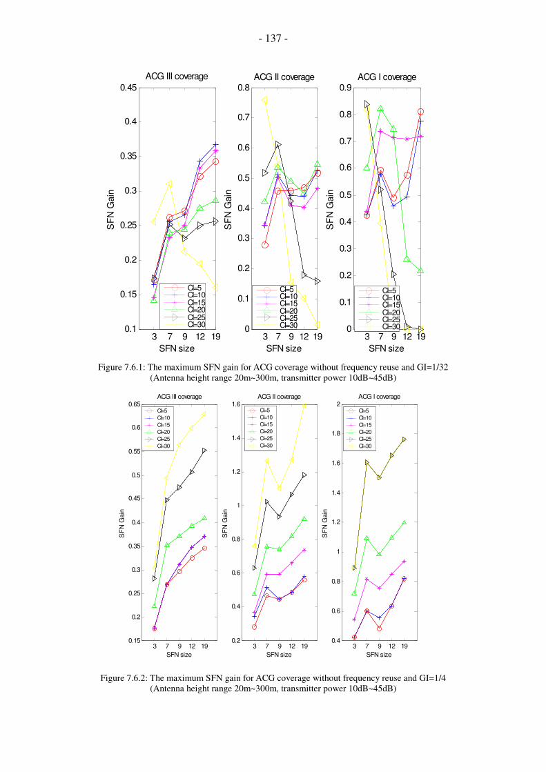
- 137 -

3 7 9 12 190.1

0.15

0.2

0.25

0.3

0.35

0.4

0.45

SFN size

SF

N G

ain

ACG III coverage

CI=5CI=10CI=15CI=20CI=25CI=30

3 7 9 12 190

0.1

0.2

0.3

0.4

0.5

0.6

0.7

0.8

SFN size

SF

N G

ain

ACG II coverage


3 7 9 12 190

0.1

0.2

0.3

0.4

0.5

0.6

0.7

0.8

0.9

SFN size

SF

N G

ain

ACG I coverage


Figure 7.6.1: The maximum SFN gain for ACG coverage without frequency reuse and GI=1/32

(Antenna height range 20m~300m, transmitter power 10dB~45dB)

3 7 9 12 190.15

0.2

0.25

0.3

0.35

0.4

0.45

0.5

0.55

0.6

0.65

SFN size

SF

N G

ain

ACG III coverage

CI=5

CI=10

CI=15

CI=20

CI=25

CI=30

3 7 9 12 190.2

0.4

0.6

0.8

1

1.2

1.4

1.6

SFN size

SF

N G

ain

ACG II coverage

CI=5

CI=10

CI=15

CI=20

CI=25

CI=30

3 7 9 12 190.4

0.6

0.8

1

1.2

1.4

1.6

1.8

2

SFN size

SF

N G

ain

ACG I coverage

CI=5

CI=10

CI=15

CI=20

CI=25

CI=30

Figure 7.6.2: The maximum SFN gain for ACG coverage without frequency reuse and GI=1/4

(Antenna height range 20m~300m, transmitter power 10dB~45dB)

- 138 -

7.6.2 SFN gain with a frequency reuse:

In the presence of co-channel interference, the equation for SFN gain is:

1 -R

RGain

MFN

SFNnSFNn = (7-6-2)

RSFNn is the optimal cell radius of a SFN size of n with reuse factor m. RMFN is the

optimal cell radius of a MFN with the same reuse factor m.

Due to the high co-channel interference coming from the two SFNs outside, no cell

radius for some C/I thresholds can satisfy some ACG coverage requirements. For

example, Figure A11-1 shows the optimal cell radius of a SFN of size 3 and reuse factor 3 for ACG I coverage, but for a higher C/I threshold, no radius satisfies this

ACG I coverage requirement. Because of this, the SFN gain only can be shown in

those cases where optimal cell radius can be derived. For a MFN with the same reuse

factor as the SFN the optimal radius does not exist for some ACG coverage

requirements and high C/I thresholds in the lower range of the antenna height and

transmitter power, and the SFN gain cannot be derived in these cases. So Figure 12-1

to Figure 12-7 only show some SFN gains in the coordinate range.

Observations:

1. The location of highest SFN gain is not fixed in middle or the corner of the coordinate box area.

2. For an area that has SFN gains, the gains are all positive.

3. An optimal cell radius for MFN and SFN size = 3 does not exit for some high

coverage requirements and high C/I thresholds, It exits for SFN size = 7; this

means the high density of SFN transmitters can improve the cell coverage.

4. Because optimal cell radiuses for the MFN with high C/I thresholds at some

reuse factors do not exit for some antenna height and transmitter power

combinations, the corresponding SFN gain cannot be computed. Figure 7.6.3

and 7.6.4 shows some SFN gains in terms of the different reuse factors and

ACG coverage requirements. The SFN gain can be computed for most of the simulation points. For C/I = 5 and C/I = 10 in Figure 7.6.3, the SFN gain

decreases with increasing reuse factor for ACG III coverage. Figure 7.6.4

shows that the SFN gain with C/I = 5 decreases while for C/I=10 it slightly

increases with increasing reuse factor.

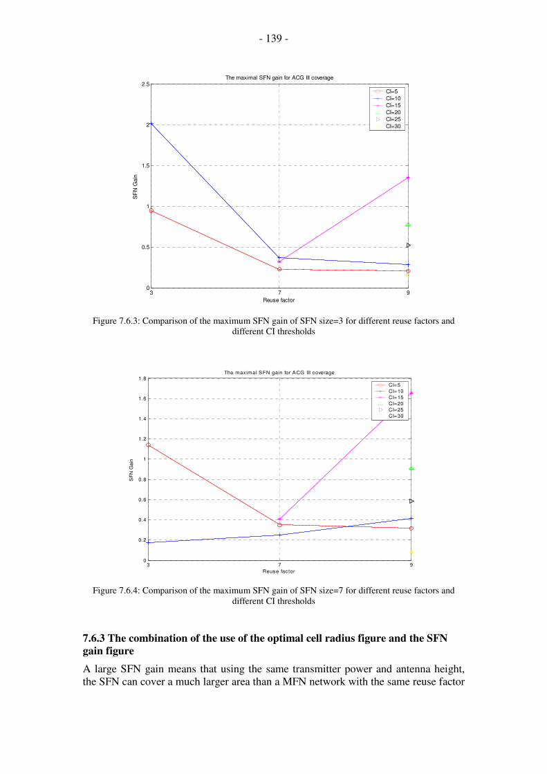
- 139 -

3 7 90

0.5

1

1.5

2

2.5

Reuse factor

SF

N G

ain

The maximal SFN gain for ACG III coverage

CI=5

CI=10

CI=15

CI=20

CI=25

CI=30

Figure 7.6.3: Comparison of the maximum SFN gain of SFN size=3 for different reuse factors and

different CI thresholds

3 7 90

0.2

0.4

0.6

0.8

1

1.2

1.4

1.6

1.8

Reuse fac tor

SF

N G

ain

The maximal SFN gain for ACG III coverage

CI=5

CI=10

CI=15

CI=20

CI=25

CI=30

Figure 7.6.4: Comparison of the maximum SFN gain of SFN size=7 for different reuse factors and

different CI thresholds

7.6.3 The combination of the use of the optimal cell radius figure and the SFN

gain figure

A large SFN gain means that using the same transmitter power and antenna height,

the SFN can cover a much larger area than a MFN network with the same reuse factor

- 140 -

and the whole network can benefit from the deployment of a single frequency

network.

Though there is a range of antenna height and transmitter power combinations that

give a predefined cell radius, the best choice is the combination that gives the largest

SFN gain at the same time. For example, Figure 7.6.5 shows the optimal point for the

8km radius at the SFN gain = 0.7. The optimal point means that the SFN can get the maximum coverage gain compared with the MFN with the same antenna height and

transmit power. In other words, if the MFN is deployed instead of the SFN using the

same antenna height and transmitter power and the other network parameters are kept

the same, the MFN cell radius will shrink to RSFN/(1+G), here RSFN is the SFN cell

radius, and G means the SFN gain.

10 15 20 25 30 35 40 45

50

100

150

200

250

300


Ante

nna h

eig

ht(

m)

C/I=20;Optimal cell radius of SFN size=7; Reuse factor=7; ACGIII Guard interval=1/4

6000

6000

6000

8000

8000

8000

0.1

0.1

0.10.1 0.1

0.1

0.1

0. 2

0.2

0.2 0.2 0.2

0.2

0.2

0.2

0.3

0.3

0.3

0.3

0.3

0.3 0.3

0.40.4

0.4

0.4 0.40.4

0.5

0.50.5

0.60.6

0.70.8

Optimal point

Figure 7.6.5: A combination graph of SFN gain and SFN optimal cell radius for ACG III coverage

(the red and purple line represents the contour of the optimal cell radius, the light blue line represents

the contour of the SFN gain)

7.7 Conclusions

In this chapter, a coverage planning process for DVB-H SFNs has been presented.

Based on simulation results the network performance for different cell sizes and

frequency reuse factors was investigated for one DVB-H transmitter configuration

leading to the following conclusions:

• External and internal interference play an important role in the coverage planning and dimensioning of DVB-T/H networks.

• DVB-H network planning has an additional burst duration parameter to consider compared with DVB-T network coverage planning.

- 141 -

• For one cell radius, there is a range of transmitter power and antenna height that can achieve the predefined coverage requirement; the optimal choice of

the transmitter power and antenna height is that which gives the maximum

SFN gain.

• Increasing the number of the transmitters in a SFN can raise the C/I threshold coverage in the case of frequency reuse and ¼ guard interval.

• In the presence of inner interference (1/32 guard interval) and without frequency reuse, the SFN network cannot provide better network performance

than a single cell for some transmitter power and antenna height combinations.

The network parameters need to be carefully selected based on simulation

results and field trials.

• For the no frequency reuse case, a symmetrical topology will give better coverage for the reason of less self–interference incurred than with an

asymmetric topology.

• In the small guard interval and no frequency reuse case, for a high C/I

threshold like 25 or 30 and a high coverage requirement (ACG I or II), increasing the number of the SFN transmitters will decrease the maximum

SFN gain for the reason of increasing self-interference.

7.8 References:

[1] Prosch, T.A.; The digital audio broadcast single frequency network project in

southwest Germany; Broadcasting, IEEE Transactions on, Volume: 40, Issue 4, Dec.

1994, Pages: 238 – 246

[2] ECC REP004 Annex-Criteria for planning DVB-T

[3] Ligeti, A., and Zander, J.; Minimal cost coverage planning for single frequency

networks; Broadcasting, IEEE Transactions on, Volume: 45, Issue: 1 , March 1999; Pages:78 – 87

[4] Ligeti, A; Coverage probability estimation in single frequency networks in

presence of correlated useful and interfering components; Vehicular Technology

Conference, 1999. VTC 1999 - Fall. IEEE VTS 50th, Volume 4, 19-22 Sept. 1999;

Pages: 2408 - 2412 vol.4

[5] Terrestrial digital television planning and implementation considerations, BNP005,

third issue, summer 2001

[6] Gordon L. Stuber; Principles of Mobile Communication; second edition

ISBN 7-5053-9698-6;

[7] Beaulieu, N.C.; Abu-Dayya, A.A.; McLane, P.J.; Comparison of methods of computing lognormal sum distributions and outages for digital wireless applications;

Humanity Through Communications. IEEE International Conference on, 1-5 May

1994; Page(s): 1270 -1275 vol.3

[8] European Telecommunication Standard Institute, “Digital Video Broadcasting

(DVB): Implementation guidelines for DVB terrestrial services; Transmission

aspects,” ETSI TR 101 190 V1.2.1 (2004-11)

[9] ETSI EN 300 744 V1.5.1: Digital Video Broadcasting (DVB): Framing structure,

channel coding and modulation for digital terrestrial television. (2004-06)

[10] Jukka Henriksson; “DVB-H outline”; http://www.dvb.org

- 142 -

[11] ITU-R Recommendation P.1546: Method for point-to-area predictions for

terrestrial services in the frequency range 30 MHz to 3 000 MHz

http://www.itu.int/itudoc/itu-r/rec/p/index.html.

[12] Stanko Perpar; Technical characteristics of digital systems; BR Seminar;18-19

September 2003.

[13] Jean-Jacques Giutot; Network configurations; BR Seminar; 18-19 September 2003.

[14].Digital video broadcasting: DVB-H implementation guide; ETSI TR 102 377;

v1.1.1; 02, 2005;

[15] http://www.kathrein.de/en/mca/index.htm; 30-08-2005;

[16] ERC/EBC Report on planning and introduction terrestrial digital (DVB-T) in

Europe. Izmir, December, 1997;

[17] J. Doeven; Planning of Single Frequency Network; ITU/EBU workshop on

Digital broadcasting; Sofia; 8-10 June, 2005

[18] Chia-Lu Ho; Calculating the mean and variance of power sums with two log-

normal components; Vehicular Technology, IEEE Transactions on; Volume 44, Issue 4, Nov. 1995 Page(s): 756 – 762

[19] S.C.Schwartz and Y.S.Yeh, “On the distribution function and moments of power

sums with log-normal components”, Bell Syst. Tech. J., vol. 61, no. 7, pp. 1441-1462,

Sept. 1982

[20] Rebhan, R. and Zander, J.; On the outage probability in single frequency

networks for digital broadcasting; Broadcasting, IEEE Transactions on; Volume

39, Issue 4, Dec. 1993 Page(s): 395 - 401

- 143 -

Chapter 8 DVB-T/-H receiver performance

In order to validate the performance of the RF frontend incorporated in the DVM400

test probe, and to verify some of the conclusions for network planning, a number of

tests were carried out in accordance with the test methodology described in the DVB-

H Validation Task Force final report [ETSI TR 102 401 v1.1.1 (2005-06)].

8.1 Test set-up

Figure 8.1: Test set-up for diversity measurements

The test set-up includes two test signal generators Type SFQ from R&S which are

operated in such a way that the first one provides the channel encoding plus channel

simulation (fading) and up-conversion to RF, while for the second only fading and up-

conversion are used.

The signals RF1 and RF2 generated by this set-up are synchronised in frequency and

are bit synchronous. Since the channel simulators are free-running, there is no

correlation between the propagation profiles of the two signals.

Up-converter

Up-converter

- 144 -

8.2 Transmission mode

For the comparison tests a 16QAM CR=2/3 GI=1/4 mode was chosen that had already

been used for the DVB-H VTF tests. It is representative since it is already used for

DVB-T transmission in several countries. The net bit rate for this mode is 13.27 Mbps.

In the table below the minimum C/N requirements are given for static propagation

profiles (Gaussian, Rice, Raleigh) which are described in detail in the DVB-T standard (EN 300 744).

For a dynamic channel such as TU6 that was used for the comparison measurements,

the minimal C/N requirements are significantly higher.

Figure 8.2: Overview of DVB-T modes

8.3 Test results

For the comparison tests, a failure criterion was defined as in the DVB-H VTF test

methodology, i.e. the C/N values were measured for a Frame Error Rate (FER) of 5 %

and for a MFER (FER after MPE FEC) of 5 %.

These were the settings:

Output level SFQ -40dBm RF frequency 666MHz

FFT-Mode 8K

Code rate 2/3

Guard Interval 1/4

Modulation 16 QAM

Data rate DVB-H Multiplex 4.00MBit/s

Data rate DVB-H Service 512kBit/s

Burst duration 520ms

MPE-FEC Code rate 3/4

MPE-FEC rows 768 Propagation profile TU 6

Ts Ts Ts TsFFT ICS Tu 1/4 1/8 1/16 1/328K 1 116 Hz 896 µs 1120 µs 1008 µs 952 µs 924 µs4K 2 232 Hz 448 µs 560 µs 504 µs 476 µs 462 µs2K 4 464 Hz 224 µs 280 µs 252 µs 238 µs 231 µs

C/N C/N C/N Modulation Bit RateGaussian Rice Rayleigh Constellation CR 1/4 1/8 1/16 1/32

3,1 dB 3,6 dB 5,4 dB QPSK 1/2 4,98 Mbps 5,53 Mbps 5,85 Mbps 6,03 Mbps4,9 dB 5,7 dB 8,4 dB QPSK 2/3 6,64 Mbps 7,37 Mbps 7,81 Mbps 8,04 Mbps5,9 dB 6,8 dB 10,7 dB QPSK 3/4 7,46 Mbps 8,29 Mbps 8,78 Mbps 9,05 Mbps6,9 dB 8,0 dB 13,1 dB QPSK 5/6 8,29 Mbps 9,22 Mbps 9,76 Mbps 10,05 Mbps7,7 dB 8,7 dB 16,3 dB QPSK 7/8 8,71 Mbps 9,68 Mbps 10,25 Mbps 10,56 Mbps8,8 dB 9,6 dB 11,2 dB 16QAM 1/2 9,95 Mbps 11,06 Mbps 11,71 Mbps 12,06 Mbps

11,1 dB 11,6 dB 14,2 dB 16QAM 2/3 13,27 Mbps 14,75 Mbps 15,61 Mbps 16,09 Mbps12,5 dB 13,0 dB 16,7 dB 16QAM 3/4 14,93 Mbps 16,59 Mbps 17,56 Mbps 18,10 Mbps13,5 dB 14,4 dB 19,3 dB 16QAM 5/6 16,59 Mbps 18,43 Mbps 19,52 Mbps 20,11 Mbps13,9 dB 15,0 dB 22,8 dB 16QAM 7/8 17,42 Mbps 19,35 Mbps 20,49 Mbps 21,11 Mbps14,4 dB 14,7 dB 16,0 dB 64QAM 1/2 14,93 Mbps 16,59 Mbps 17,56 Mbps 18,10 Mbps16,5 dB 17,1 dB 19,3 dB 64QAM 2/3 19,91 Mbps 22,12 Mbps 23,42 Mbps 24,13 Mbps18,0 dB 18,6 dB 21,7 dB 64QAM 3/4 22,39 Mbps 24,88 Mbps 26,35 Mbps 27,14 Mbps19,3 dB 20,0 dB 25,3 dB 64QAM 5/6 24,88 Mbps 27,65 Mbps 29,27 Mbps 30,16 Mbps20,1 dB 21,0 dB 27,9 dB 64QAM 7/8 26,13 Mbps 29,03 Mbps 30,74 Mbps 31,67 Mbps

8 MHz

- 145 -

The measurement value and the corresponding figures show the dependencies

between Doppler shift and required C/N. In the DVB-H VTF report, the following

diagram is used to visualise the performance for DVB-T modes (without MPE FEC)

and DVB-H modes (including MPE FEC).

Figure 8.3: Characterisation of a DVB-T/-H receiver in TR 102 401

• FER 5%, Test duration 100 Bursts

• MFER 5%, Test duration 100 Bursts

Doppler shift w/o diversity with diversity

1 Hz 17.5 dB 13.0 dB

2 Hz 17.0 dB 12.5 dB

10 Hz 16.5 dB 11.5 dB

20 Hz 16.0 dB 12.0 dB

fd max (50dB) 60 Hz 75 Hz

MINMINT2T2

fd,max/2fd,max/2

C/NC/N

T1T1

T3T3

2 / 5 / 10Hz2 / 5 / 10Hz

T4T4

MIN+3dBMIN+3dB

fd,3dBfd,3dB fd,maxfd,max

T0T0T0

DopplerDoppler

FrequencyFrequency

NotNot

WorkingWorking

AreaArea

Working

Reception

Area

WorkingWorking

ReceptionReception

AreaArea

DVB-H GainArea

DVBDVB--H GainH Gain

AreaArea

H1H1

H3H3

H2H2H4H4

H5H5H6H6

Portable Mobile

H0H0

MINMINT2T2

fd,max/2fd,max/2

C/NC/N

T1T1

T3T3

2 / 5 / 10Hz2 / 5 / 10Hz

T4T4

MIN+3dBMIN+3dB

fd,3dBfd,3dB fd,maxfd,max

T0T0T0

DopplerDoppler

FrequencyFrequency

NotNot

WorkingWorking

AreaArea

Working

Reception

Area

WorkingWorking

ReceptionReception

AreaArea

DVB-H GainArea

DVBDVB--H GainH Gain

AreaArea

H1H1

H3H3

H2H2H4H4

H5H5H6H6

Portable Mobile

H0H0

Doppler shift w/o diversity with diversity

1 Hz 19.5 dB 14.0 dB

2 Hz 19.5 dB 14.0 dB

10 Hz 21.5 dB 15.5 dB

20 Hz 22.5 dB 15.5 dB

fd max (50dB) 40 Hz 60 Hz

- 146 -

The tendency in the diagram above can be summarised as follows:

• The usage for MPE FEC increases the tolerable Doppler shift for mobile reception by about 40 %, and reduces the required C/N by about 6 dB.

• The usage of diversity produces an effect in the same order of magnitude: plus 40 % tolerable Doppler shift and minus 6 dB required C/N.

• In the first case the price is paid by a reduction of the usable bit rate, in the

second case the effort is paid for in hardware and software.

• The combination of both strategies accumulates both gains.

• For very low Doppler shifts the gain in C/N is reduced. It remains to be investigated if this effect occurs in a similar way when a new profile for

outdoor/ indoor reception at pedestrian speed is used. Such a profile is still under development. First results point to the conclusion that TU6 is less

applicable in such circumstances.

This is in line with the findings of the DVB-H VTF report. It confirms that the RF

front-end represents the state-of-the-art. It also confirms some basic assumptions for

the planning of DVB-H networks in comparison with planning for DVB-T networks.

- 147 -

Chapter 9 Conclusions

In this document by means of simulations and measurements, network engineering

rules have been defined that will enable a more efficient use of broadcast spectrum by

contributing to the definition of protection ratio and frequency allocation management.

Co-working of 2G/3G/4G telecom networks and broadcast networks on the same site

has been addressed to cut down on roll out expenses of future services and networks.

From the present state-of-the-art planning processes and regulatory aspects, the

following have been addressed:

o Description of the spectrum use for analogue TV,

o Description of the theoretical DVB-T network dimensioning

o Description of frequency planning in the real world and during the simulcast

period

o Possible scenarios for analogue networks switch off

o Densification of networks that are not dedicated to reception in mobility

o Identification of rules for “cellularized” DVB-T/H planning (ERP, Reuse

pattern, etc.)

o Related spectrum demands

o Coverage comparison in defined scenarios

Finally, the potential impact of diversity receivers on spectrum planning is briefly

discussed at the end of this chapter.

In overview the main conclusions drawn from this document chapter by chapter are as

follows:

In chapter 2 it was shown that it is not clear that spectrum will be available for DVB-H services in all the countries of the European Union after the analogue switch-off. In

the context of what follows this means that in the planning of DVB-H networks

particular attention must be paid to using spectrum efficiently. On a more positive

note, in Brazil an important example of an emerging economy adopting digital TV

where there is not anticipated to be any shortage of spectrum for DVB-H.

In chapter 3 the cell ranges for different DVB-T/-H reception modes were given for

different transmitter heights / powers and for rural as well as for urban environments.

It was shown that large SFNs where the size of the whole network is large in

comparison to the guard interval are possible without severe self-interference. For

multi-frequency networks (MFN) based on a hexagonal cell layout different C/I (carrier-to-interference) estimates were given for the use of omnidirectional transmit

antennas. C/I values for different transmitter heights and cluster sizes were given for

different cell radii and propagation environments at the terminal. As the most

effective means of lowering the cluster size and thus obtaining the lowest number of

frequencies required to deliver full area coverage, the illumination of MFN cells by

SFNs consisting of three 120° sectorized transmitters was considered. Compared with

the use of omnidirectional antennas in the cell centre there is no need for additional

transmitter locations, but the cluster size can be reduced significantly at the expense

of two additional transmitters and antennas at each transmitter site.

A positive SFN Gain under same parameter configuration means that the SFN network is effective for such a configuration; it can cover a bigger area compared with

- 148 -

using the same number of MFN transmitters with no frequency reuse. In chapter 4 it

was shown that SFN gain can be substantial: from 20% in a worst case scenario, to

70% in the case of optimised site location, ERP and heights, for three transmitters.

SFN gain is even larger when small sites are deployed: little ERP on a large number

of sites will increase the SFN gain. Although the SFN gain can be quite impressive in

the case of a large number of sites, with values over 100% in the case of 10+ sites, the cost of deployment must be taken into account, and it was anticipated that the cost of

the site multiplication would not be compensated for by the SFN gain. Following on

from this in Chapter 5 using the TDF proprietary radio planning tool and a TDF

proprietary cost function based on CAPEX it was shown that while the SFN gain can

be quite important in the case of a large number of sites, the cost of the site

multiplication is not compensated for by the SFN gain.

Chapter 6 presented cositing issues between the DVB-H system and radiocom

services (GSM900, GSM1800, and UMTS). The main topic was Electro-Magnetic

Compatibility (EMC) between radio systems. The isolation required between systems,

to maintain an acceptable Quality of Service (QoS) was derived from radio equipment

specifications and possible cositing architectures were proposed in terms of antenna

spacing.

Chapter 7 described an approach to studying coverage planning and dimensioning in

DVB-H. The planning of network coverage is currently divided into two steps, the

first one is the physical layer simulation which models the receiver sensitivity with different physical layer parameters under different kinds of channels and produces a

table of SNR values for different parameter combinations; the second step is the

coverage planning process using the SNR values produced in step one to simulate the

coverage ratio for different network topologies and network level parameters. Chapter

7 mainly addressed the latter step showing that the proposed approach can potentially

deliver significant insights into the planning process.

Chapter 8 reported the results of a number of tests carried out in accordance with the

test methodology described in the DVB-H Validation Task Force final report [ETSI

TR 102 401 v1.1.1 (2005-06)]. The results confirm some basic assumptions for the

planning of DVB-H networks in comparison with planning for DVB-T networks.

It has to be emphasised that this deliverable represents only a first step in developing

a systematic approach to the planning of DVB-H networks. Not only do many of the

results reported need to be developed further new issues will emerge as DVB-H

matures. For example, it is probable that diversity will have to be taken into account

in the planning of DVB-H networks in the longer term, as diversity has already to be

taken into consideration for DVB-T networks. At the moment, the commercial

importance of diversity DVB-T receivers for mobile reception is for the scenarios of

in the car and indoor portable reception. This aspect of mobile reception was taken

into consideration for the network planning in Germany. To allow mobile reception in

the car, with diversity, in Germany, an 8k, 16 QAM network was set up. If diversity receivers for DVB-H were widely available DVB-H network planning for indoor

portable reception could allow an interesting trade off between coverage (e.g. 90% of

people in a given area with one antenna receivers) and additional expenses for

diversity receivers (extra costs of about 50 Euro? per receiver) to extend the coverage

to e.g. 95% of the people (i.e. only 5% of the people would have to buy the more

expensive receiver). However, at the moment, diversity is not a serious option for

DVB-H network planning.

- 149 -

- 150 -

Appendices

A1. Frequency allocation in Germany [26]

The following table lists the frequency allocation in the VHF to UHF band in

Germany, for details of the frequency allocation in other bands, please refer to [26].

Table A1: Frequency allocation between 40MHz – 900MHz in Germany

FREQUENCY BAND ALLOCATIONS APPLICATIONS

39.85 - 41.0 MHz MOBILE Fixed

Defence systems Point-to-Multipoint Model control (40.66 - 40.7 MHz) Non-specific SRDs (40.66 - 40.7 MHz) On-site paging (40.66 - 40.7 MHz) Short Range Devices (40.66 - 40.7 MHz) Telemetry (civil) (40.66 - 40.7 MHz) Model control (40.71 - 40.74 MHz) Model control (40.76 - 40.79 MHz) Model control (40.81 - 40.84 MHz) Model control (40.86 - 40.89 MHz) Model control (40.91 - 40.94 MHz) Model control (40.96 - 40.99 MHz)


Defence systems (41.0 - 47.0 MHz) Fixed links (41.0 - 47.0 MHz)

46.0 - 47.0 MHz MOBILE Fixed Radiolocation

Defence systems (41.0 - 47.0 MHz) Fixed links (41.0 - 47.0 MHz) Wind profilers

47.0 - 50.08 MHz BROADCASTING LAND MOBILE Radiolocation

TV analogue (terrestrial) (47.0 - 68.0 MHz) Tactical mobile (47.0 - 68.0 MHz) Wind profilers (47.0 - 68.0 MHz)

50.08 - 51.0 MHz

BROADCASTING LAND MOBILE Amateur Radiolocation

TV analogue (terrestrial) (47.0 - 68.0 MHz) Tactical mobile (47.0 - 68.0 MHz) Wind profilers (47.0 - 68.0 MHz) Amateur

51.0 - 68.0 MHz BROADCASTING LAND MOBILE Radiolocation

TV analogue (terrestrial) (47.0 - 68.0 MHz) Tactical mobile (47.0 - 68.0 MHz) Wind profilers (47.0 - 68.0 MHz)

68.0 - 70.0 MHz LAND MOBILE

PMR/PAMR (68.0 - 68.04 MHz) PMR/PAMR (68.08 - 68.62 MHz) Railway applications (68.62 - 69.56 MHz) PMR/PAMR (69.56 - 69.92 MHz) PMR/PAMR (69.94 - 69.98 MHz)

70.0 - 74.2 MHz FIXED MOBILE except aeronautical mobile

Defence systems Tactical mobile Railway applications (70.04 - 70.9 MHz) PMR/PAMR (70.2 - 70.22 MHz) PMR/PAMR (70.42 - 70.44 MHz) PMR/PAMR (71.0 - 71.7 MHz) PMR/PAMR (72.34 - 72.76 MHz)

74.2 - 74.8 MHz LAND MOBILE Emergency services (74.205 - 74.785 MHz)

74.8 - 75.2 MHz AERONAUTICAL RADIONAVIGATION ILS


Emergency services (75.205 - 77.465 MHz) SAP/SAB and ENG/OB (77.5 - 77.8 MHz)

- 151 -

77.8 - 84.0 MHz MOBILE except aeronautical mobile Fixed

PMR/PAMR (77.88 - 78.42 MHz) Railway applications (78.42 - 78.7 MHz) Tactical mobile (78.7 - 84.0 MHz) Railway applications (80.04 - 80.9 MHz) PMR/PAMR (81.0 - 81.7 MHz) PMR/PAMR (82.34 - 82.76 MHz)


Emergency services (84.005 - 84.585 MHz) Emergency services (84.585 - 85.005 MHz) Emergency services (85.005 - 85.265 MHz) SAP/SAB and ENG/OB (87.275 - 87.5 MHz)

87.5 - 108.0 MHz BROADCASTING FM sound analogue Point-to-Multipoint

108.0 - 117.975 MHz AERONAUTICAL RADIONAVIGATION ILS (108.0 - 111.975 MHz) VOR (111.975 - 117.975 MHz)

117.975 - 136.0 MHz AERONAUTICAL MOBILE (R) Aeronautical Mobile-Satellite (R)

Aeronautical communications (117.975 - 137.0 MHz) Aeronautical satcoms (117.975 - 137.0 MHz) Space Operations (117.975 - 137.0 MHz) Space research (117.975 - 137.0 MHz) EPIRBs (121.45 - 121.55 MHz) SAR (communications) (123.05 - 123.15 MHz)

136.0 - 137.0 MHz

AERONAUTICAL MOBILE (R) Aeronautical Mobile-Satellite (R) Meteorological-Satellite (space-to-Earth)

Aeronautical communications (117.975 - 137.0 MHz) Aeronautical satcoms (117.975 - 137.0 MHz) Space Operations (117.975 - 137.0 MHz) Space research (117.975 - 137.0 MHz) Weather satellites

137.0 - 137.025 MHz

METEOROLOGICAL-SATELLITE (space-to-Earth) MOBILE-SATELLITE (space-to-Earth) SPACE OPERATION (space-to-Earth) SPACE RESEARCH (space-to-Earth) Mobile except aeronautical mobile (R)

Defence systems S-PCS Space Operations Space research Weather satellites

137.025 - 137.175 MHz

METEOROLOGICAL-SATELLITE (space-to-Earth) SPACE OPERATION (space-to-Earth) SPACE RESEARCH (space-to-Earth) Mobile except aeronautical mobile (R) Mobile-Satellite (space-to-Earth)


137.175 - 137.825 MHz

METEOROLOGICAL-SATELLITE (space-to-Earth) MOBILE-SATELLITE (space-to-Earth) SPACE OPERATION (space-to-Earth) SPACE RESEARCH (space-to-Earth) Mobile except aeronautical mobile (R)

Space Operations (137.175 - 137.275 MHz) AGA communications (military) S-PCS Space research Weather satellites

137.825 - 138.0 MHz

METEOROLOGICAL-SATELLITE (space-to-Earth) SPACE OPERATION (space-to-Earth) SPACE RESEARCH (space-to-Earth) Mobile except aeronautical mobile (R) Mobile-Satellite (space-to-Earth)


138.0 - 144.0 MHz AERONAUTICAL MOBILE (OR) LAND MOBILE

AGA communications (military) Land mobile Tactical mobile

- 152 -

144.0 - 146.0 MHz AMATEUR AMATEUR-SATELLITE

Amateur Amateur-satellite


PMR/PAMR (146.0 - 146.36 MHz) Railway applications (146.36 - 146.92 MHz) PMR/PAMR (146.92 - 148.0 MHz)

148.0 - 149.9 MHz

MOBILE except aeronautical mobile (R) SPACE OPERATION (Earth-to-space) Mobile-Satellite (Earth-to-space)

PMR/PAMR (148.0 - 148.4 MHz) S-PCS Space Operations PMR/PAMR (148.4 - 149.01 MHz) Telemetry (civil) (149.01875 - 149.03125 MHz) PMR/PAMR (149.01875 - 149.05625 MHz) PMR/PAMR (149.06 - 149.14 MHz) PMR/PAMR (149.14 - 149.88 MHz) On-site paging (149.88 - 149.9 MHz)

149.9 - 150.05 MHz MOBILE-SATELLITE (Earth-to-space) RADIONAVIGATION-SATELLITE

S-PCS Satellite navigation systems

150.05 - 156.7625 MHz

MOBILE except aeronautical mobile

PMR/PAMR (150.24 - 150.54 MHz) PMR/PAMR (150.56 - 151.06 MHz) Radio Microphones (150.98 - 151.06 MHz) On-site paging (151.06 - 151.08 MHz) Telemetry (civil) (151.08 - 151.1 MHz) Radio Microphones (151.1 - 151.16 MHz) PMR/PAMR (151.1 - 151.72 MHz) PMR/PAMR (151.9 - 152.02 MHz) PMR/PAMR (152.04 - 152.1 MHz) PMR/PAMR (152.28 - 152.76 MHz) PMR/PAMR (152.78 - 153.0 MHz) PMR/PAMR (153.0 - 153.74 MHz) PMR/PAMR (153.74 - 155.96 MHz) GMDSS (156.0 - 156.7625 MHz) Maritime communications (156.0 - 156.7625 MHz) PMR/PAMR (156.015 - 156.035 MHz)

156.7625 - 156.8375 MHz

MARITIME MOBILE (distress and calling)

Maritime communications GMDSS (156.795 - 156.805 MHz)

156.8375 - 174.0 MHz MOBILE except aeronautical mobile

174.0 - 223.0 MHz BROADCASTING Radio Microphones T-DAB TV analogue (terrestrial)

223.0 - 230.0 MHz BROADCASTING Fixed Mobile

Radio Microphones T-DAB TV analogue (terrestrial)


AGA communications (military) Tactical radio relay


AGA communications (military) Tactical radio relay EPIRBs (242.95 - 243.05 MHz) Satellite systems (military) (242.95 - 243.05 MHz)

272.0 - 273.0 MHz MOBILE SPACE OPERATION (space-to-Earth) Fixed

AGA communications (military) Space Operations Tactical radio relay



312.0 - 315.0 MHz MOBILE Fixed Mobile-Satellite (Earth-to-space)

AGA communications (military) Feeder links Tactical radio relay



322.0 - 328.6 MHz MOBILE AGA communications (military)

- 153 -

Fixed Radio Astronomy

Radio astronomy Tactical radio relay



AGA communications (military) Tactical radio relay Emergency services (380.0 - 383.0 MHz) ISM (380.0 - 387.0 MHz)

387.0 - 390.0 MHz MOBILE Fixed Mobile-Satellite (space-to-Earth)

AGA communications (military) MSS Earth stations Tactical radio relay


Emergency services (390.0 - 393.0 MHz) AGA communications (military) Tactical radio relay


S-PCS Satellite navigation systems

400.05 - 400.15 MHz STANDARD FREQUENCY AND TIME SIGNAL-SATELLITE

Standard Frequency and Time Signal-Satellite

400.15 - 401.0 MHz

METEOROLOGICAL-SATELLITE (space-to-Earth) METEOROLOGICAL AIDS MOBILE-SATELLITE (space-to-Earth) SPACE RESEARCH (space-to-Earth) Space Operation (space-to-Earth)

Meteorology S-PCS Space Operations Space research Subscriber access excluding MWS

401.0 - 402.0 MHz

METEOROLOGICAL-SATELLITE (Earth-to-space) METEOROLOGICAL AIDS SPACE OPERATION (space-to-Earth)

Meteorology Space Operations Weather satellites Subscriber access excluding MWS (401.1 - 402.0 MHz)

402.0 - 403.0 MHz METEOROLOGICAL-SATELLITE (Earth-to-space) METEOROLOGICAL AIDS

Medical implants Weather satellites Telemetry (civil) (402.1 - 403.0 MHz) Sondes (402.2 - 403.0 MHz)

403.0 - 406.0 MHz METEOROLOGICAL AIDS

Medical implants (403.0 - 405.0 MHz) Sondes Subscriber access excluding MWS (405.15 - 406.0 MHz)

406.0 - 406.1 MHz MOBILE-SATELLITE (Earth-to-space) GMDSS

406.1 - 410.0 MHz LAND MOBILE RADIO ASTRONOMY

Subscriber access excluding MWS (406.1 - 407.0 MHz) PMR/PAMR Radio astronomy

410.0 - 420.0 MHz LAND MOBILE Fixed

Fixed links (410.0 - 410.8 MHz) PMR/PAMR PMR/PAMR (410.00625 - 415.00625 MHz) Fixed links (415.0 - 415.8 MHz) PMR/PAMR (415.80625 - 416.61875 MHz) PMR/PAMR (416.63125 - 417.36875 MHz) PMR/PAMR (417.38125 - 419.71875 MHz) Railway applications (419.72 - 419.8 MHz) PMR/PAMR (419.80625 - 419.99375 MHz) PMR/PAMR (419.99375 - 420.0 MHz)


PMR/PAMR (420.0 - 420.00625 MHz) Fixed links (420.0 - 420.8 MHz) PMR/PAMR PMR/PAMR (420.00625 - 425.00625 MHz) Fixed links (425.0 - 425.8 MHz) PMR/PAMR (425.80625 - 426.61875 MHz)

- 154 -

PMR/PAMR (426.63125 - 427.36875 MHz) PMR/PAMR (427.38125 - 429.71875 MHz) PMR/PAMR (429.80625 - 429.99375 MHz)

430.0 - 435.0 MHz AMATEUR

Amateur (430.0 - 440.0 MHz) Radiolocation (military) (430.0 - 440.0 MHz) Short Range Devices (433.05 - 434.79 MHz) Model control (433.0875 - 434.7625 MHz) Telemetry (civil) (433.0875 - 434.7625 MHz) Non-specific SRDs (433.92 - 434.79 MHz)

435.0 - 438.0 MHz AMATEUR Amateur-Satellite

Amateur (430.0 - 440.0 MHz) Radiolocation (military) (430.0 - 440.0 MHz) Amateur

438.0 - 440.0 MHz AMATEUR Amateur (430.0 - 440.0 MHz) Radiolocation (military) (430.0 - 440.0 MHz)





449.75 - 449.9625 MHz

LAND MOBILE Fixed Space Operation (Earth-to-space) Space Research (Earth-to-space)

449.9625 - 450.25 MHz

LAND MOBILE Space Operation (Earth-to-space) Space Research (Earth-to-space)


470.0 - 494.0 MHz BROADCASTING Land Mobile Radiolocation

Wind profilers Radio Microphones (470.0 - 608.0 MHz) DVB-T (470.0 - 790.0 MHz) TV analogue (terrestrial) (470.0 - 790.0 MHz) PMR/PAMR (477.0 - 790.0 MHz) Radio Microphones (477.0 - 790.0 MHz)

494.0 - 608.0 MHz BROADCASTING Land Mobile

Radio Microphones (470.0 - 608.0 MHz) DVB-T (470.0 - 790.0 MHz) TV analogue (terrestrial) (470.0 - 790.0 MHz) PMR/PAMR (477.0 - 790.0 MHz) Radio Microphones (477.0 - 790.0 MHz)

608.0 - 614.0 MHz BROADCASTING Land Mobile Radio Astronomy

DVB-T (470.0 - 790.0 MHz) TV analogue (terrestrial) (470.0 - 790.0 MHz) PMR/PAMR (477.0 - 790.0 MHz) Radio Microphones (477.0 - 790.0 MHz) Radio astronomy

614.0 - 790.0 MHz BROADCASTING Land Mobile

DVB-T (470.0 - 790.0 MHz) TV analogue (terrestrial) (470.0 - 790.0 MHz) PMR/PAMR (477.0 - 790.0 MHz) Radio Microphones (477.0 - 790.0

- 155 -

MHz) Radio Microphones


Tactical radio relay (790.0 - 814.0 MHz)


Tactical radio relay (790.0 - 814.0 MHz) Radio Microphones (798.0 - 814.0 MHz) Subscriber access excluding MWS (812.0 - 818.0 MHz) DVB-T (814.0 - 838.0 MHz) Subscriber access excluding MWS (824.0 - 828.0 MHz) Tactical radio relay (830.0 - 862.0 MHz) Subscriber access excluding MWS (857.0 - 862.0 MHz)


Subscriber access excluding MWS (862.0 - 863.0 MHz) Tactical radio relay (862.0 - 868.0 MHz) Radio Microphones (863.0 - 865.0 MHz) Wireless Audio Applications (863.0 - 865.0 MHz) CT2 (864.1 - 868.1 MHz) Alarms (868.0 - 868.6 MHz) Alarms (868.6 - 868.7 MHz) Alarms (868.7 - 869.2 MHz) Subscriber access excluding MWS (869.0 - 873.0 MHz) Alarms (869.2 - 869.25 MHz) Alarms (869.25 - 869.3 MHz) Alarms (869.4 - 869.65 MHz) Alarms (869.65 - 869.7 MHz) Alarms (869.7 - 870.0 MHz) Land mobile (870.0 - 876.0 MHz) GSM-R (876.0 - 880.0 MHz) Tactical radio relay (880.0 - 885.0 MHz) CT1+ (885.0 - 887.0 MHz) Tactical radio relay (887.0 - 890.0 MHz)


GSM (890.1 - 914.9 MHz) Land mobile (915.0 - 921.0 MHz) GSM-R (921.0 - 925.0 MHz) Tactical radio relay (925.0 - 930.0 MHz) CT1+ (930.0 - 932.0 MHz) Tactical radio relay (932.0 - 935.0 MHz) GSM (935.1 - 959.9 MHz)

- 156 -

A2. Frequency allocation in France [26]:

The following table lists the frequency allocation in the VHF to UHF band in France,

for details of the frequency allocation in other bands, Please refer to [26].

Table A2: Frequency allocation between 40MHz – 900MHz in France [26]

FREQUENCY BAND ALLOCATIONS APPLICATIONS

39.4 - 40.65 MHz FIXED MOBILE SPACE RESEARCH (active)

Defence systems PMR/PAMR

40.65 - 41.0 MHz FIXED MOBILE SPACE RESEARCH (active)

Defence systems Short Range Devices

41.0 - 41.5 MHz FIXED MOBILE

Cordless telephones Fixed links PMR/PAMR


Defence systems

47.0 - 68.0 MHz BROADCASTING TV analogue (terrestrial)




Fixed links PMR/PAMR


Defence systems








Defence systems Fixed links


Defence systems Model control




Defence systems





Defence systems




Defence systems




Fixed links Paging

87.5 - 108.0 MHz BROADCASTING FM sound analogue

108.0 - 117.975 MHz AERONAUTICAL RADIONAVIGATION VOR

117.975 - 136.0 MHz AERONAUTICAL MOBILE (R) Aeronautical communications

136.0 - 137.0 MHz AERONAUTICAL MOBILE (R) SPACE RESEARCH (space-to-Earth)

Aeronautical communications

137.0 - 138.0 MHz AERONAUTICAL MOBILE (OR) Defence systems

- 157 -

METEOROLOGICAL-SATELLITE (space-to-Earth) MOBILE-SATELLITE (space-to-Earth) SPACE OPERATION SPACE RESEARCH (space-to-Earth)

Satellite systems (civil) Space Operations Space research Weather satellites

138.0 - 144.0 MHz AERONAUTICAL MOBILE (OR) SPACE RESEARCH (space-to-Earth)

Defence systems

144.0 - 146.0 MHz AMATEUR AMATEUR-SATELLITE

Amateur Amateur-satellite

146.0 - 148.0 MHz FIXED MOBILE except aeronautical mobile (R)

Defence systems

148.0 - 148.825 MHz

FIXED MOBILE except aeronautical mobile (R) MOBILE-SATELLITE (Earth-to-space) SPACE OPERATION

Defence systems Satellite systems (civil) Space Operations

148.825 - 149.9 MHz

FIXED MOBILE except aeronautical mobile (R) MOBILE-SATELLITE (Earth-to-space) SPACE OPERATION

Fixed links Satellite systems (civil) Space Operations

149.9 - 150.05 MHz MOBILE-SATELLITE (Earth-to-space) RADIONAVIGATION-SATELLITE SPACE RESEARCH (space-to-Earth)

Defence systems Satellite systems (civil) Space research

150.05 - 150.4 MHz FIXED MOBILE except aeronautical mobile RADIO ASTRONOMY

Fixed links Land mobile Radio astronomy


Fixed links PMR/PAMR Radio astronomy


Defence systems Maritime military systems Radio astronomy

153.0 - 153.425 MHz FIXED METEOROLOGICAL AIDS MOBILE except aeronautical mobile (R)

Defence systems

153.425 - 154.0 MHz FIXED METEOROLOGICAL AIDS MOBILE except aeronautical mobile (R)



Defence systems Fixed links Maritime communications PMR/PAMR


Defence systems EPIRBs

156.7625 - 156.8375 MHz

MARITIME MOBILE Maritime communications




Defence systems Maritime communications PMR/PAMR











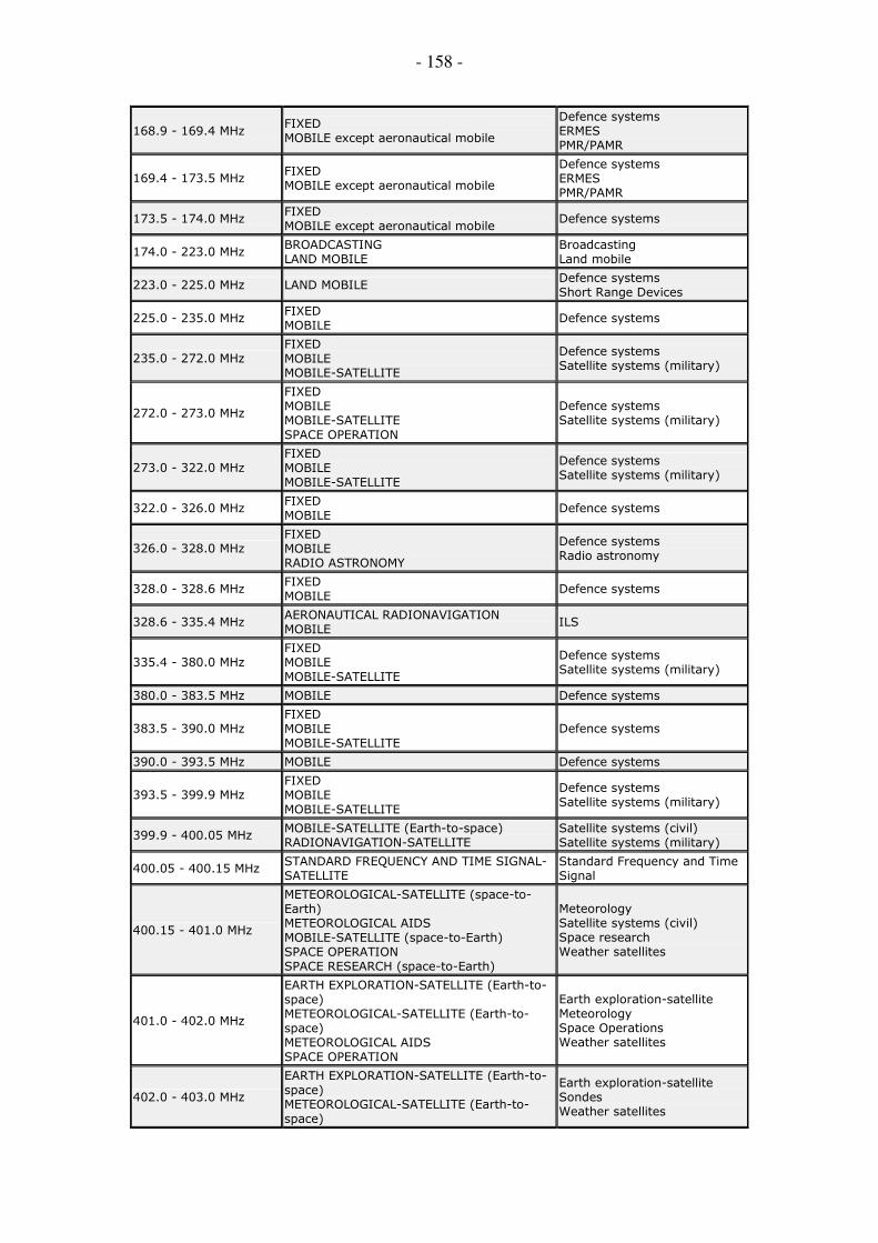
- 158 -


Defence systems ERMES PMR/PAMR


Defence systems ERMES PMR/PAMR


Defence systems

174.0 - 223.0 MHz BROADCASTING LAND MOBILE

Broadcasting Land mobile

223.0 - 225.0 MHz LAND MOBILE Defence systems Short Range Devices


Defence systems

235.0 - 272.0 MHz FIXED MOBILE MOBILE-SATELLITE

Defence systems Satellite systems (military)

272.0 - 273.0 MHz

FIXED MOBILE MOBILE-SATELLITE SPACE OPERATION





Defence systems

326.0 - 328.0 MHz FIXED MOBILE RADIO ASTRONOMY

Defence systems Radio astronomy


Defence systems

328.6 - 335.4 MHz AERONAUTICAL RADIONAVIGATION MOBILE

ILS



380.0 - 383.5 MHz MOBILE Defence systems


Defence systems

390.0 - 393.5 MHz MOBILE Defence systems




Satellite systems (civil) Satellite systems (military)

400.05 - 400.15 MHz STANDARD FREQUENCY AND TIME SIGNAL-SATELLITE

Standard Frequency and Time Signal

400.15 - 401.0 MHz

METEOROLOGICAL-SATELLITE (space-to-Earth) METEOROLOGICAL AIDS MOBILE-SATELLITE (space-to-Earth) SPACE OPERATION SPACE RESEARCH (space-to-Earth)

Meteorology Satellite systems (civil) Space research Weather satellites

401.0 - 402.0 MHz

EARTH EXPLORATION-SATELLITE (Earth-to-space) METEOROLOGICAL-SATELLITE (Earth-to-space) METEOROLOGICAL AIDS SPACE OPERATION

Earth exploration-satellite Meteorology Space Operations Weather satellites

402.0 - 403.0 MHz

EARTH EXPLORATION-SATELLITE (Earth-to-space) METEOROLOGICAL-SATELLITE (Earth-to-space)

Earth exploration-satellite Sondes Weather satellites

- 159 -

METEOROLOGICAL AIDS

403.0 - 406.0 MHz METEOROLOGICAL AIDS Sondes

406.0 - 406.1 MHz MOBILE-SATELLITE (Earth-to-space) EPIRBs

406.1 - 408.0 MHz MOBILE except aeronautical mobile RADIO ASTRONOMY

PMR/PAMR Radio astronomy

408.0 - 410.0 MHz MOBILE except aeronautical mobile RADIO ASTRONOMY

Defence systems Radio astronomy

410.0 - 414.5 MHz FIXED MOBILE except aeronautical mobile SPACE RESEARCH (space-to-space)

Defence systems Space research

414.5 - 420.0 MHz MOBILE except aeronautical mobile SPACE RESEARCH (space-to-space)


420.0 - 424.5 MHz FIXED MOBILE except aeronautical mobile RADIOLOCATION

Defence systems



430.0 - 432.0 MHz

AMATEUR FIXED MOBILE except aeronautical mobile RADIOLOCATION

Radiolocation (military)

432.0 - 434.0 MHz

AMATEUR EARTH EXPLORATION-SATELLITE FIXED MOBILE except aeronautical mobile RADIOLOCATION SPACE OPERATION

Radiolocation (military)

434.0 - 435.0 MHz

AMATEUR EARTH EXPLORATION-SATELLITE RADIOLOCATION SPACE OPERATION

Amateur Radiolocation (military)

435.0 - 438.0 MHz

AMATEUR AMATEUR-SATELLITE (Earth-to-space) EARTH EXPLORATION-SATELLITE RADIOLOCATION


438.0 - 440.0 MHz AMATEUR RADIOLOCATION



Defence systems

441.5 - 443.55 MHz MOBILE except aeronautical mobile RADIOLOCATION

Defence systems


Defence systems

444.5 - 447.0 MHz MOBILE except aeronautical mobile RADIOLOCATION

PMR/PAMR

447.0 - 449.775 MHz

FIXED MOBILE except aeronautical mobile RADIOLOCATION SPACE OPERATION SPACE RESEARCH (Earth-to-space)


449.775 - 450.025 MHz SPACE OPERATION SPACE RESEARCH (Earth-to-space)

Space Operations Space research

450.025 - 451.5 MHz

FIXED MOBILE SPACE OPERATION SPACE RESEARCH (Earth-to-space)

Defence systems

451.5 - 454.5 MHz MOBILE PMR/PAMR


Defence systems

456.0 - 460.0 MHz MOBILE PMR/PAMR

- 160 -

460.0 - 463.55 MHz

EARTH EXPLORATION-SATELLITE (space-to-Earth) FIXED METEOROLOGICAL-SATELLITE (space-to-Earth) MOBILE

Defence systems



464.5 - 466.0 MHz

EARTH EXPLORATION-SATELLITE (space-to-Earth) FIXED METEOROLOGICAL-SATELLITE (space-to-Earth) MOBILE


466.0 - 470.0 MHz

EARTH EXPLORATION-SATELLITE (space-to-Earth) METEOROLOGICAL-SATELLITE (space-to-Earth) MOBILE

PMR/PAMR


TV analogue (terrestrial)


TV analogue (terrestrial)

830.0 - 854.0 MHz MOBILE except aeronautical mobile Defence systems



869.2 - 869.7 MHz MOBILE except aeronautical mobile Alarms


880.0 - 890.0 MHz MOBILE except aeronautical mobile GSM

890.0 - 915.0 MHz MOBILE except aeronautical mobile GSM

- 161 -

A3: k-LNM method from [1]

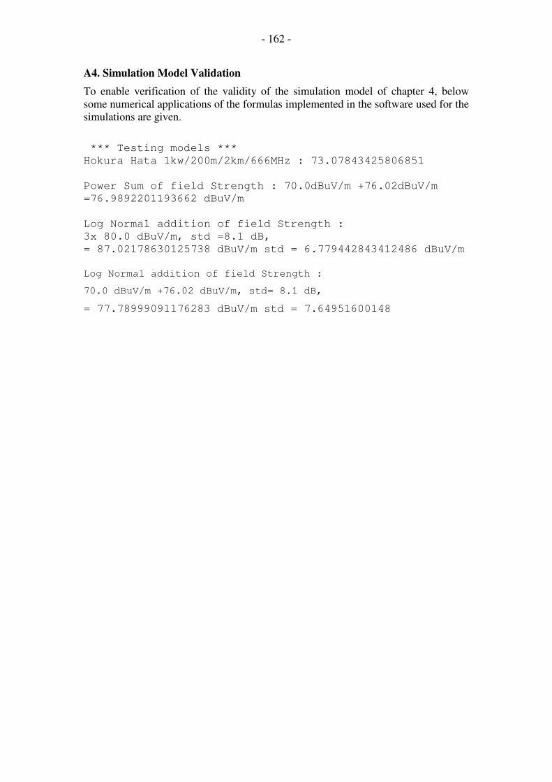
- 162 -

A4. Simulation Model Validation

To enable verification of the validity of the simulation model of chapter 4, below

some numerical applications of the formulas implemented in the software used for the

simulations are given.

*** Testing models ***

Hokura Hata 1kw/200m/2km/666MHz : 73.07843425806851

Power Sum of field Strength : 70.0dBuV/m +76.02dBuV/m

=76.9892201193662 dBuV/m

Log Normal addition of field Strength :

3x 80.0 dBuV/m, std =8.1 dB,

= 87.02178630125738 dBuV/m std = 6.779442843412486 dBuV/m

Log Normal addition of field Strength :

70.0 dBuV/m +76.02 dBuV/m, std= 8.1 dB,

= 77.78999091176283 dBuV/m std = 7.64951600148

- 163 -

A5. Site Configurations

Configuration 1: HTx = 150 m, ERP = 5 kW, 3 sites

Fictitious site Latitude Longitude

Site 0 598 000 2 430 558

Site 1 604 000 2 430 558

Site 2 601 000 2 425 192

Table A4.1: Site coordinates

Configuration 2: HTx = 75 m, ERP = 400 W, 10 sites


Site0 598 000 2 430 558 Site1 599 000 2 430 558 Site2 600 000 2 430 558 Site3 601 000 2 430 558 Site4 598 500 2 429 680 Site5 599 500 2 429 680 Site6 600 500 2 429 680 Site7 599 000 2 428 803 Site8 600 000 2 428 803 Site9 599 500 2 427 925


Configuration 3: HTx = 50 m, ERP = 100 W, 15 sites


Site0 598 000 2 430 558 Site1 598 400 2 430 558 Site2 598 800 2 430 558 Site3 599 200 2 430 558 Site4 598 200 2 430 200 Site5 598 600 2 430 200 Site6 599 000 2 430 200 Site7 598 400 2 429 842 Site8 598 800 2 429 842 Site9 598 600 2 429 484

Site10 599 600 2 430 558 Site11 599 400 2 430 200 Site12 599 200 2 429 842 Site13 599 000 2 429 484 Site14 598 800 2 429 126


- 164 -

A6. The optimal radius for one single cell

The following figures are drawn using the contour line representation and based on

the simulation results.

The figures below give the optimal radius for one single cell that is the basis of the

SFN comparison.

10 20 30 40

50

100

150

200

250

300

Ante

nna h

eig

ht(

m)

C/I=5

5000

10000

10000

15000

20000

25000

30000

10 20 30 40

50

100

150

200

250

300

Ante

nna h

eig

ht(

m)

C/I=10

10000

20000

10 20 30 40

50

100

150

200

250

300

Ante

nna h

eig

ht(

m)

C/I=15

0

50

00

5000

10000

15000

20000

10 20 30 40

50

100

150

200

250

300

Ante

nna h

eig

ht(

m)

C/I=20

0

50

00

5000

10000

15000

10 20 30 40

50

100

150

200

250

300


Ante

nna h

eig

ht(

m)

C/I=25

5000

10000

Optimal cell radius of single transmitter cell; ACGI

10 20 30 40

50

100

150

200

250

300


Ante

nna h

eig

ht(

m)

C/I=30

0

0

20

00

2000

4000

6000

8000

10000

Figure A6-1. The optimal cell radius of a single transmitter cell; ACG I coverage

10 20 30 40

50

100

150

200

250

300

Ante

nna h

eig

ht(

m)

C/I=5

5000 10000

10000

15000

15000

20000

25000300003500040

000

10 20 30 40

50

100

150

200

250

300

Ante

nna h

eig

ht(

m)

C/I=10

5000

10000

10000

15000

20000

25000

30000

10 20 30 40

50

100

150

200

250

300

Ante

nna h

eig

ht(

m)

C/I=15

50

00

5000

10000

15000

20000

25000

10 20 30 40

50

100

150

200

250

300

Ante

nna h

eig

ht(

m)

C/I=20

0

50

00

5000

10000

15000

20000

10 20 30 40

50

100

150

200

250

300


Ante

nna h

eig

ht(

m)

C/I=25

0

5000

10000

15000

Optimal cell radius of single transmitter cell; ACGII

10 20 30 40

50

100

150

200

250

300


Ante

nna h

eig

ht(

m)

C/I=30

5000

10000

Figure A6-2. The optimal cell radius of a single transmitter cell; ACG II coverage

- 165 -

10 20 30 40

50

100

150

200

250

300

Ante

nna h

eig

ht(

m)

C/I=5

10000

20000

20000

30000

40000

50000

60000

10 20 30 40

50

100

150

200

250

300

Ante

nna h

eig

ht(

m)

C/I=10

10000

20000

30000

40000

50000

10 20 30 40

50

100

150

200

250

300

Ante

nna h

eig

ht(

m)

C/I=15

10000 20000

30000

40000

10 20 30 40

50

100

150

200

250

300

Ante

nna h

eig

ht(

m)

C/I=20

5000

10000

10000

15000

20000

25000

30000

35000

10 20 30 40

50

100

150

200

250

300


Ante

nna h

eig

ht(

m)

C/I=25

10000

20000

30000

Optimal cell radius of single transmitter cell; ACGIII

10 20 30 40

50

100

150

200

250

300


Ante

nna h

eig

ht(

m)

C/I=30

0

50

00

5000

10000

15000

20000

Figure A6-3. The optimal cell radius of a single transmitter cell; ACG III coverage

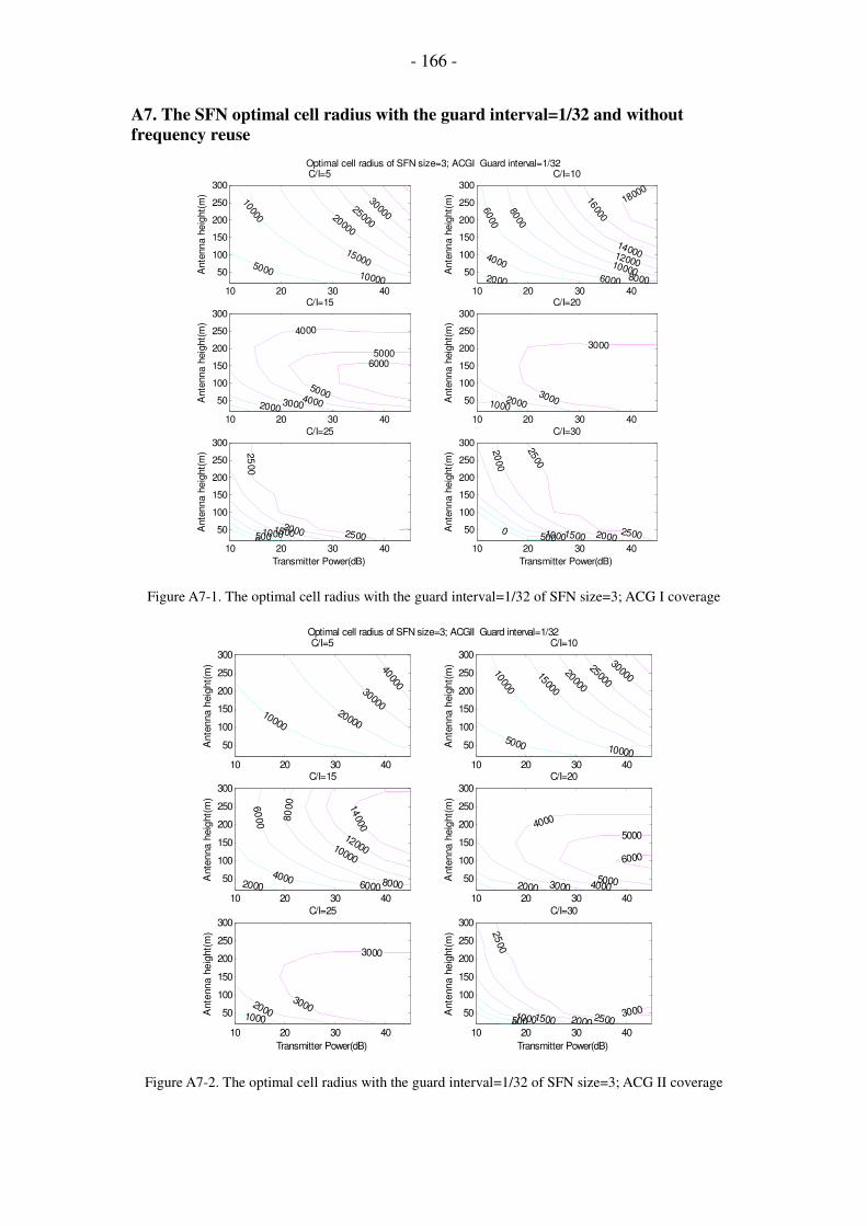
- 166 -


frequency reuse

10 20 30 40

50

100

150

200

250

300

Ante

nna h

eig

ht(

m)

C/I=5

5000

10000

10000

15000

20000

25000

30000

10 20 30 40

50

100

150

200

250

300

Ante

nna h

eig

ht(

m)

C/I=10

2000

4000

6000

6000

8000

8000

10000

12000

14000

16000

18000

10 20 30 40

50

100

150

200

250

300

Ante

nna h

eig

ht(

m)

C/I=15

20003000

4000

4000

5000

5000

6000

10 20 30 40

50

100

150

200

250

300

Ante

nna h

eig

ht(

m)

C/I=20

10002000

3000

3000

10 20 30 40

50

100

150

200

250

300


Ante

nna h

eig

ht(

m)

C/I=25

0500100015002000

25

00

2500

Optimal cell radius of SFN size=3; ACGI Guard interval=1/32

10 20 30 40

50

100

150

200

250

300


Ante

nna h

eig

ht(

m)

C/I=30

050010001500

20

00

2000

2500

2500

Figure A7-1. The optimal cell radius with the guard interval=1/32 of SFN size=3; ACG I coverage

10 20 30 40

50

100

150

200

250

300

Ante

nna h

eig

ht(

m)

C/I=5

10000

20000

30000

40000

10 20 30 40

50

100

150

200

250

300

Ante

nna h

eig

ht(

m)

C/I=10

5000

10000

10000

15000

20000

25000

30000

10 20 30 40

50

100

150

200

250

300

Ante

nna h

eig

ht(

m)

C/I=15

2000

4000

60

00

6000

80

00

8000

10000

12000

14000

10 20 30 40

50

100

150

200

250

300

Ante

nna h

eig

ht(

m)

C/I=20

2000 3000 4000

4000

5000

5000

6000

10 20 30 40

50

100

150

200

250

300


Ante

nna h

eig

ht(

m)

C/I=25

1000

2000

3000

3000

Optimal cell radius of SFN size=3; ACGII Guard interval=1/32

10 20 30 40

50

100

150

200

250

300


Ante

nna h

eig

ht(

m)

C/I=30

050010001500 2000

25

00

25003000

Figure A7-2. The optimal cell radius with the guard interval=1/32 of SFN size=3; ACG II coverage

- 167 -

10 20 30 40

50

100

150

200

250

300

Ante

nna h

eig

ht(

m)

C/I=5

10000

20000

30000 40000

5000060000

10 20 30 40

50

100

150

200

250

300

Ante

nna h

eig

ht(

m)

C/I=10

10000

20000

30000

40000

50000

10 20 30 40

50

100

150

200

250

300

Ante

nna h

eig

ht(

m)

C/I=15

10000

20000

30000

40000

10 20 30 40

50

100

150

200

250

300

Ante

nna h

eig

ht(

m)

C/I=20

5000

10000

10000

15000

20000

25000

30000

10 20 30 40

50

100

150

200

250

300


Ante

nna h

eig

ht(

m)

C/I=25

50

00

5000

10000

15000

20000

Optimal cell radius of SFN size=3; ACGIII Guard interval=1/32

10 20 30 40

50

100

150

200

250

300


Ante

nna h

eig

ht(

m)

C/I=30

2000

3000

40

00

4000

5000

5000

6000

6000

7000

80

00

Figure A7-3. The optimal cell radius with the guard interval=1/32 of SFN size=3; ACG III coverage

10 20 30 40

50

100

150

200

250

300

Ante

nna h

eig

ht(

m)

C/I=5

5000

10000

15000

20000

25000

30000

35000

10 20 30 40

50

100

150

200

250

300

Ante

nna h

eig

ht(

m)

C/I=10

4000

6000

8000

10000

12000

10 20 30 40

50

100

150

200

250

300

Ante

nna h

eig

ht(

m)

C/I=15

50004500

4000

3500

3000

10 20 30 40

50

100

150

200

250

300

Ante

nna h

eig

ht(

m)

C/I=20

3000

2500

2000

10 20 30 40

50

100

150

200

250

300


Ante

nna h

eig

ht(

m)

C/I=25

2500

2000

1500


10 20 30 40

50

100

150

200

250

300


Ante

nna h

eig

ht(

m)

C/I=30

1600

14001200

1000


- 168 -

10 20 30 40

50

100

150

200

250

300

Ante

nna h

eig

ht(

m)

C/I=5

50000

400003000020000

10000

10 20 30 40

50

100

150

200

250

300

Ante

nna h

eig

ht(

m)

C/I=1035000

300002500020000

1500010000

5000

10 20 30 40

50

100

150

200

250

300

Ante

nna h

eig

ht(

m)

C/I=15

10000

9000

8000

7000

6000

5000

4000

200010 20 30 40

50

100

150

200

250

300

Ante

nna h

eig

ht(

m)

C/I=20

4000

3000

2000

10 20 30 40

50

100

150

200

250

300


Ante

nna h

eig

ht(

m)

C/I=25

3000

2500

2000

1500


10 20 30 40

50

100

150

200

250

300


Ante

nna h

eig

ht(

m)

C/I=30

20001500

500


10 20 30 40

50

100

150

200

250

300

Ante

nna h

eig

ht(

m)

C/I=5

7000060000

500004000030000

20000

10000

10 20 30 40

50

100

150

200

250

300

Ante

nna h

eig

ht(

m)

C/I=10

6000050000

400003000020000

10000

10 20 30 40

50

100

150

200

250

300

Ante

nna h

eig

ht(

m)

C/I=15

400003000020000

10000

10 20 30 40

50

100

150

200

250

300

Ante

nna h

eig

ht(

m)

C/I=20

30000

2000010000

5000

10 20 30 40

50

100

150

200

250

300


Ante

nna h

eig

ht(

m)

C/I=25

1000090008000

70006

000

50

00

3000


10 20 30 40

50

100

150

200

250

300


Ante

nna h

eig

ht(

m)

C/I=30

5000

4000

3000

2000


- 169 -


frequency reuse

10 20 30 40

50

100

150

200

250

300

Ante

nna h

eig

ht(

m)

C/I=5

5000

10000

10000

15000

20000

2500030000

10 20 30 40

50

100

150

200

250

300

Ante

nna h

eig

ht(

m)

C/I=10

5000

10000

15000

2000025000

10 20 30 40

50

100

150

200

250

300

Ante

nna h

eig

ht(

m)

C/I=15

5000

5000

10000

15000

20000

10 20 30 40

50

100

150

200

250

300

Ante

nna h

eig

ht(

m)

C/I=20

0

5000

5000

10000

15000

10 20 30 40

50

100

150

200

250

300


Ante

nna h

eig

ht(

m)

C/I=25

0

5000

10000

15000


10 20 30 40

50

100

150

200

250

300


Ante

nna h

eig

ht(

m)

C/I=30

0

20

00

2000

4000

6000

8000

1000012000


10 20 30 40

50

100

150

200

250

300

Ante

nna h

eig

ht(

m)

C/I=5

10000

20000

30000

40000

10 20 30 40

50

100

150

200

250

300

Ante

nna h

eig

ht(

m)

C/I=10

5000

10000

10000

15000

20000

250003000035000

10 20 30 40

50

100

150

200

250

300

Ante

nna h

eig

ht(

m)

C/I=15

5000

10000

15000

20000

25000

10 20 30 40

50

100

150

200

250

300

Ante

nna h

eig

ht(

m)

C/I=20

5000

5000

10000

15000

20000

10 20 30 40

50

100

150

200

250

300


Ante

nna h

eig

ht(

m)

C/I=25

0

5000

5000

10000

15000


10 20 30 40

50

100

150

200

250

300


Ante

nna h

eig

ht(

m)

C/I=30

0

5000

10000

15000


- 170 -

10 20 30 40

50

100

150

200

250

300

Ante

nna h

eig

ht(

m)

C/I=5

10000 20000

30000

40000

50000

60000

10 20 30 40

50

100

150

200

250

300

Ante

nna h

eig

ht(

m)

C/I=10

10000

20000

20000

30000

40000

50000

10 20 30 40

50

100

150

200

250

300

Ante

nna h

eig

ht(

m)

C/I=15

10000

20000

30000

40000

10 20 30 40

50

100

150

200

250

300

Ante

nna h

eig

ht(

m)

C/I=20

5000

10000

10000

15000

20000

250003000035000

10 20 30 40

50

100

150

200

250

300


Ante

nna h

eig

ht(

m)

C/I=25

5000

10000

10000

15000

20000

2500030000


10 20 30 40

50

100

150

200

250

300


Ante

nna h

eig

ht(

m)

C/I=30

50

00

5000

10000

15000

20000

25000

Figure A8-3. The optimal radius with the guard interval=1/4 of SFN size=3; ACG III coverage

10 20 30 40

50

100

150

200

250

300

Ante

nna h

eig

ht(

m)

C/I=5

5000

1000015000

20000

25000

30000

35000

10 20 30 40

50

100

150

200

250

300

Ante

nna h

eig

ht(

m)

C/I=10

5000

10000

10000

15000

20000

25000

10 20 30 40

50

100

150

200

250

300

Ante

nna h

eig

ht(

m)

C/I=15

5000

10000

15000

20000

10 20 30 40

50

100

150

200

250

300

Ante

nna h

eig

ht(

m)

C/I=20

5000

5000

10000

15000

10 20 30 40

50

100

150

200

250

300


Ante

nna h

eig

ht(

m)

C/I=25

0

2000

4000

4000

6000

8000

10000

12000


10 20 30 40

50

100

150

200

250

300


Ante

nna h

eig

ht(

m)

C/I=30

02000

20

00

4000

4000

60008000

1000012000


- 171 -

10 20 30 40

50

100

150

200

250

300

Ante

nna h

eig

ht(

m)

C/I=5

10000

20000

30000

40000

10 20 30 40

50

100

150

200

250

300

Ante

nna h

eig

ht(

m)

C/I=10

5000 10000

10000

15000

200002500030000

35000

10 20 30 40

50

100

150

200

250

300

Ante

nna h

eig

ht(

m)

C/I=15

5000

10000

10000

15000

20000

25000

10 20 30 40

50

100

150

200

250

300

Ante

nna h

eig

ht(

m)

C/I=20

5000

10000

15000

20000

10 20 30 40

50

100

150

200

250

300


Ante

nna h

eig

ht(

m)

C/I=25

0

5000

5000

10000

15000


10 20 30 40

50

100

150

200

250

300


Ante

nna h

eig

ht(

m)

C/I=30

0

2000

4000

4000

6000

8000

10000

12000


10 20 30 40

50

100

150

200

250

300

Ante

nna h

eig

ht(

m)

C/I=5

10000

2000030000

40000

50000

60000

10 20 30 40

50

100

150

200

250

300

Ante

nna h

eig

ht(

m)

C/I=10

10000

20000

20000

30000

4000050000

10 20 30 40

50

100

150

200

250

300

Ante

nna h

eig

ht(

m)

C/I=15

10000

20000

30000

40000

10 20 30 40

50

100

150

200

250

300

Ante

nna h

eig

ht(

m)

C/I=20

5000 10000

10000

1500020000

25000

30000

35000

10 20 30 40

50

100

150

200

250

300


Ante

nna h

eig

ht(

m)

C/I=25

5000

10000

10000

15000

20000

25000


10 20 30 40

50

100

150

200

250

300


Ante

nna h

eig

ht(

m)

C/I=30

5000

5000

10000

15000

20000


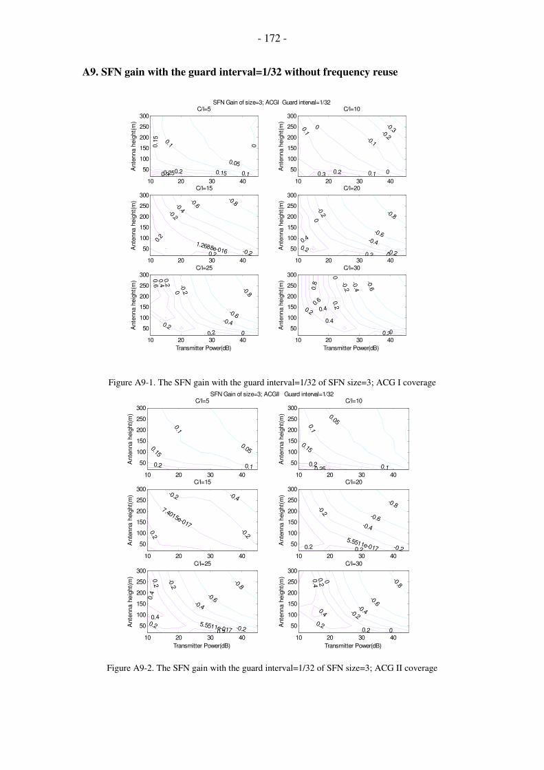
- 172 -

A9. SFN gain with the guard interval=1/32 without frequency reuse

10 20 30 40

50

100

150

200

250

300

Ante

nna h

eig

ht(

m)

C/I=5

0

0.05

0.1

0.1

0.1

5

0.150.20.250.310 20 30 40

50

100

150

200

250

300

Ante

nna h

eig

ht(

m)

C/I=10

-0.3-0.2-0.1

0

00.1

0.1

0.20.3

10 20 30 40

50

100

150

200

250

300

Ante

nna h

eig

ht(

m)

C/I=15

-0.8-0.6-0.4-0.2

-0.2

1.2688e-0160.2

0.2

10 20 30 40

50

100

150

200

250

300

Ante

nna h

eig

ht(

m)

C/I=20

-0.8

-0.6-0.4

-0.2

-0.2

0

0

0.20.2

0.4

10 20 30 40

50

100

150

200

250

300


Ante

nna h

eig

ht(

m)

C/I=25

-0.8

-0.6-0.4

-0.20

0

0.2

0.2

0.2

0.4

0.6

SFN Gain of size=3; ACGI Guard interval=1/32

10 20 30 40

50

100

150

200

250

300


Ante

nna h

eig

ht(

m)

C/I=30

-0.6

-0.4

-0.2

0

0

0.2

0.2

0.2

0.4

0.4

0.6

0.8

Figure A9-1. The SFN gain with the guard interval=1/32 of SFN size=3; ACG I coverage

10 20 30 40

50

100

150

200

250

300

Ante

nna h

eig

ht(

m)

C/I=5

0.05

0.1

0.1

0.15

0.2

10 20 30 40

50

100

150

200

250

300

Ante

nna h

eig

ht(

m)

C/I=10

0.05

0.1

0.1

0.15

0.20.25

10 20 30 40

50

100

150

200

250

300

Ante

nna h

eig

ht(

m)

C/I=15

-0.4-0.2

-0.2

7.4015e-017

0.2

10 20 30 40

50

100

150

200

250

300

Ante

nna h

eig

ht(

m)

C/I=20

-0.8

-0.6-0.4

-0.2

-0.2

5.5511e-0170.20.2

10 20 30 40

50

100

150

200

250

300


Ante

nna h

eig

ht(

m)

C/I=25

-0.8

-0.6-0.4

-0.2

-0.25.5511e-017

0.2

0.20.2

0.4

0.4

SFN Gain of size=3; ACGII Guard interval=1/32

10 20 30 40

50

100

150

200

250

300


Ante

nna h

eig

ht(

m)

C/I=30

-0.8

-0.6-0.4-0.2

0

0

0.2

0.20.2

0.4

0.4

Figure A9-2. The SFN gain with the guard interval=1/32 of SFN size=3; ACG II coverage

- 173 -

10 20 30 40

50

100

150

200

250

300

Ante

nna h

eig

ht(

m)

C/I=5

0.04

0.060.08

0.080.1

0.1

0.120.14

10 20 30 40

50

100

150

200

250

300

Ante

nna h

eig

ht(

m)

C/I=10

0.02

0.04

0.06

0.08

0.08

0.1

0.10.120.14

10 20 30 40

50

100

150

200

250

300

Ante

nna h

eig

ht(

m)

C/I=15

0

0.020.04

0.06

0.06

0.08

0.080.1

0.1

0.120.1410 20 30 40

50

100

150

200

250

300

Ante

nna h

eig

ht(

m)

C/I=20

-0.05

0

00.05

0.050.10.1

10 20 30 40

50

100

150

200

250

300


Ante

nna h

eig

ht(

m)

C/I=25

-0.3-0.2

-0.2

-0.1

-0.1

3.7007e-0170.1

SFN Gain of size=3; ACGIII Guard interval=1/32

10 20 30 40

50

100

150

200

250

300


Ante

nna h

eig

ht(

m)

C/I=30

-0.8-0.6

-0.4

-0.2

-0.21.2688e-016

0.2

Figure A9-3. The SFN gain with the guard interval=1/32 of SFN size=3; ACG III coverage

10 20 30 40

50

100

150

200

250

300

Ante

nna h

eig

ht(

m)

C/I=5

0

0.1

0.2

0.20.30.40.510 20 30 40

50

100

150

200

250

300

Ante

nna h

eig

ht(

m)

C/I=10

-0.6-0.4-0.2

-0.2

0

00.2

0.2

0.4

10 20 30 40

50

100

150

200

250

300

Ante

nna h

eig

ht(

m)

C/I=15

-0.8

-0.6

-0.4

-0.4

-0.2

-0.2

5.5511e-017

0.20.2

0.410 20 30 40

50

100

150

200

250

300

Ante

nna h

eig

ht(

m)

C/I=20

-0.8

-0.6

-0.4

-0.4

-0.2

-0.2

0

00.2

0.2

0.4

0.6

10 20 30 40

50

100

150

200

250

300


Ante

nna h

eig

ht(

m)

C/I=25

-0.8

-0.6

-0.4

-0.4

-0.2

-0.2

5.5511e-017

0.2

0.2

0.2

0.4


10 20 30 40

50

100

150

200

250

300


Ante

nna h

eig

ht(

m)

C/I=30

-0.8

-0.6

-0.4

-0.2

-0.2

1.2688e-016

1.2

68

8e-0

16

0.2

0.2

0.2


- 174 -

10 20 30 40

50

100

150

200

250

300

Ante

nna h

eig

ht(

m)

C/I=5

0.1

0.15

0.2

0.20.250.30.350.410 20 30 40

50

100

150

200

250

300

Ante

nna h

eig

ht(

m)

C/I=10

-0.1

00.1

0.1

0.2

0.20.30.4

10 20 30 40

50

100

150

200

250

300

Ante

nna h

eig

ht(

m)

C/I=15

-0.8-0.6-0.4

-0.2

-0.2

5.5511e-017

0.2

0.2

0.410 20 30 40

50

100

150

200

250

300

Ante

nna h

eig

ht(

m)

C/I=20

-0.8

-0.6

-0.4

-0.4-0

.2-0.2

5.5511e-017

0.20.2

0.4

10 20 30 40

50

100

150

200

250

300


Ante

nna h

eig

ht(

m)

C/I=25

-0.8

-0.6

-0.4

-0.4

-0.2

-0.20

0

0.2

0.20.4

0.4


10 20 30 40

50

100

150

200

250

300


Ante

nna h

eig

ht(

m)

C/I=30

-0.8-0

.6

-0.4

-0.4

-0.2

-0.2

5.5511e-0

17

0.2

0.20.2

0.4


10 20 30 40

50

100

150

200

250

300

Ante

nna h

eig

ht(

m)

C/I=5

0.05

0.1

0.10.15

0.2

10 20 30 40

50

100

150

200

250

300

Ante

nna h

eig

ht(

m)

C/I=10

0.05

0.1

0.10.15

0.15

0.2

10 20 30 40

50

100

150

200

250

300

Ante

nna h

eig

ht(

m)

C/I=15

9.2519e-018

0.05

0.1

0.10.150.210 20 30 40

50

100

150

200

250

300

Ante

nna h

eig

ht(

m)

C/I=20

-0.2

-0.15-0.1

-0.050

0

0.05

0.050.1

0.1

0.15

10 20 30 40

50

100

150

200

250

300


Ante

nna h

eig

ht(

m)

C/I=25

-0.8

-0.6

-0.4

-0.4

-0.2

-0.2

1.2688e-016

0.2


10 20 30 40

50

100

150

200

250

300


Ante

nna h

eig

ht(

m)

C/I=30

-0.8-0.6

-0.4

-0.4-0.2

-0.2

1.2688e-016

0.2


- 175 -

A10. The SFN gain with the guard interval=1/4 without frequency reuse

10 20 30 40

50

100

150

200

250

300

Ante

nna h

eig

ht(

m)

C/I=5

0.05

0.1

0.15

0.150.2

0.20.2

0.250.310 20 30 40

50

100

150

200

250

300

Ante

nna h

eig

ht(

m)

C/I=10

0

0.050.10.1

5

0.15

0.2

0.2

0.2

5

0.25

0.3

0.3

10 20 30 40

50

100

150

200

250

300

Ante

nna h

eig

ht(

m)

C/I=15

0

0.1

0.1

0.2

0.20.2

0.3

0.3

0.4

10 20 30 40

50

100

150

200

250

300

Ante

nna h

eig

ht(

m)

C/I=20

0.1

0.1

0.2

0.2

0.2

0.3

0.3

0.40.5

10 20 30 40

50

100

150

200

250

300


Ante

nna h

eig

ht(

m)

C/I=25

0.10.2

0.2

0.3

0.3

0.3

0.4

0.5

0.6

0.7


10 20 30 40

50

100

150

200

250

300


Ante

nna h

eig

ht(

m)

C/I=30

0.1

0.1

0. 2

0.20.2

0.3

0.3

0.3

0.4

0.40

.5 0.5

0.60

.7

0.8


10 20 30 40

50

100

150

200

250

300

Ante

nna h

eig

ht(

m)

C/I=5

0.1

0.15

0.150.2

10 20 30 40

50

100

150

200

250

300

Ante

nna h

eig

ht(

m)

C/I=10

0.05

0.1

0.1

5

0.15

0.2

0.20.20.25

10 20 30 40

50

100

150

200

250

300

Ante

nna h

eig

ht(

m)

C/I=15

0.05

0.1

0.1

0.15

0.15

0.2

0.2

0.2

5

0.25

0.3

10 20 30 40

50

100

150

200

250

300

Ante

nna h

eig

ht(

m)

C/I=20

0.1

0.1

0.2

0.2

0.2

0.3

0.4

10 20 30 40

50

100

150

200

250

300


Ante

nna h

eig

ht(

m)

C/I=25

0.1

0.1

0.2

0.2

0.20.3

0.4

0.5


10 20 30 40

50

100

150

200

250

300


Ante

nna h

eig

ht(

m)

C/I=30

0.10.2

0.2

0.2

0.3

0.3

0.4

0.4

0.5

0.6


- 176 -

10 20 30 40

50

100

150

200

250

300

Ante

nna h

eig

ht(

m)

C/I=5

0.040.06

0.08

0.080.1

0.10.12

0.140.1610 20 30 40

50

100

150

200

250

300

Ante

nna h

eig

ht(

m)

C/I=10

0.040.06

0.08

0.1

0.1

0.12

0.12

0.140.16

10 20 30 40

50

100

150

200

250

300

Ante

nna h

eig

ht(

m)

C/I=15

0.06

0.08

0.1

0.10.12

0.120.140.1610 20 30 40

50

100

150

200

250

300

Ante

nna h

eig

ht(

m)

C/I=20

0.05

0.1

0.15

0.15

10 20 30 40

50

100

150

200

250

300


Ante

nna h

eig

ht(

m)

C/I=25

0.05

0.1

0.15

0.15

0.2


10 20 30 40

50

100

150

200

250

300


Ante

nna h

eig

ht(

m)

C/I=30

0.1

0.1

0.15

0.2

0.25


10 20 30 40

50

100

150

200

250

300

Ante

nna h

eig

ht(

m)

C/I=5

0.1

0.2

0.2

0.3

0.30.40.5

10 20 30 40

50

100

150

200

250

300

Ante

nna h

eig

ht(

m)

C/I=10

0.1

0.2

0.3

0.3

0.4

0.4

0.5

0.5

10 20 30 40

50

100

150

200

250

300

Ante

nna h

eig

ht(

m)

C/I=15

0

0.1

0.1

0.2

0.2

0.3

0.30.3

0.4

0.4

0.5

0.5

0.60

.7

10 20 30 40

50

100

150

200

250

300

Ante

nna h

eig

ht(

m)

C/I=20

0

0.2

0.2

0.4 0.4

0.60.6

0.8

1

1

10 20 30 40

50

100

150

200

250

300


Ante

nna h

eig

ht(

m)

C/I=25

0

0.5

0.5

1


10 20 30 40

50

100

150

200

250

300


Ante

nna h

eig

ht(

m)

C/I=30

00.2

0.2

0.2

0.4

0.4

0.4

0.6

0.6

0.6

0.8

0.8

11.2

1.4


- 177 -

10 20 30 40

50

100

150

200

250

300

Ante

nna h

eig

ht(

m)

C/I=5

0.15

0.2

0.2

0.2

5

0.250.3

0.3

0.350.4 0.410 20 30 40

50

100

150

200

250

300

Ante

nna h

eig

ht(

m)

C/I=10

0.15

0.2

0.2

5

0.25

0. 3

0.3

0.3

5

0.35

0.4

0.4 0.4

10 20 30 40

50

100

150

200

250

300

Ante

nna h

eig

ht(

m)

C/I=15

0.1

0.1

0.2

0.2

0.3

0.30.30.4

0.4 0.4

0.5

10 20 30 40

50

100

150

200

250

300

Ante

nna h

eig

ht(

m)

C/I=20

0

0.1

0.2

0.2

0.3

0.3

0.4

0.4

0.4

0.50.

6

10 20 30 40

50

100

150

200

250

300


Ante

nna h

eig

ht(

m)

C/I=25

0

0.20.2

0.4

0.4

0.6

0.8

1


10 20 30 40

50

100

150

200

250

300


Ante

nna h

eig

ht(

m)

C/I=30

0

0.2

0.2

0.4

0.4

0.40.6

0.8

1


10 20 30 40

50

100

150

200

250

300

Ante

nna h

eig

ht(

m)

C/I=5

0.05

0.1

0.10.15

0.15

0.2

10 20 30 40

50

100

150

200

250

300

Ante

nna h

eig

ht(

m)

C/I=10

0.05

0.1

0.15

0.150.2

10 20 30 40

50

100

150

200

250

300

Ante

nna h

eig

ht(

m)

C/I=15

0.1

0.1

5

0.150.2 0.210 20 30 40

50

100

150

200

250

300

Ante

nna h

eig

ht(

m)

C/I=20

0.05

0.1

0.15

0.2

0.2

0.2

50.3

10 20 30 40

50

100

150

200

250

300


Ante

nna h

eig

ht(

m)

C/I=25

0

0.05

0.1

0.15

0.2

0.2

0.2

0.25

0.3

0.35


10 20 30 40

50

100

150

200

250

300


Ante

nna h

eig

ht(

m)

C/I=30

0.1

0.1

0.20.2 0.2

0.30.

4


- 178 -

A11. The optimal cell radius for SFN size = 3 with a Reuse factor, guard interval

= 1/4

10 15 20 25 30 35 40 45

50

100

150

200

250

300

Ante

nna h

eig

ht(

m)

C/I=5;Optimal cell radius of SFN size=3; Reuse factor=3; ACGI Guard interval=1/4

0

0 0

50

00

50005000

10

000

10000

15000

15000

20000

20000

25000

30000

Figure A11-1. The optimal cell radius of SFN size=3 and reuse factor=3; ACG I coverage; Guard

interval=1/4

10 15 20 25 30 35 40 45

50

100

150

200

250

300

Ante

nna h

eig

ht(

m)

C/I=5

0

0 0 0

10000

1000010000

20000

20000

30000

30000

40000

Optimal cell radius of SFN size=3; Reuse factor=3; ACGII Guard interval=1/4

10 15 20 25 30 35 40 45

50

100

150

200

250

300

Ante

nna h

eig

ht(

m)

C/I=10

10000

10000

20000

20000

30000

Figure A11-2. The optimal cell radius of SFN size=3 and reuse factor=3; ACG II coverage; Guard

interval=1/4

- 179 -

10 20 30 40

50

100

150

200

250

300

Ante

nna h

eig

ht(

m)

C/I=5

10000 20000

20000

30000

40000

50000

60000

10 20 30 40

50

100

150

200

250

300

Ante

nna h

eig

ht(

m)

C/I=10

10000

20000

20000

30000

40000

50000

10 20 30 40

50

100

150

200

250

300

Ante

nna h

eig

ht(

m)

C/I=15

0 0

10000

10000

20000

30000

40000

10 20 30 40

50

100

150

200

250

300

Ante

nna h

eig

ht(

m)

C/I=20

0

0

50

00

50001000015000

20000

25000

30000


10 20 30 40

50

100

150

200

250

300


Ante

nna h

eig

ht(

m)

C/I=25

05000

Figure A11-3. The optimal cell radius of SFN size=3 and reuse factor=3; ACG III coverage; Guard

interval=1/4

10 15 20 25 30 35 40 45

50

100

150

200

250

300

Ante

nna h

eig

ht(

m)

C/I=5

000 50005000

5000

10000

1000010000

15000

15000

15000

20000

20000

25000

25000

30000

35000

10 15 20 25 30 35 40 45

50

100

150

200

250

300

Ante

nna h

eig

ht(

m)

C/I=10

0

0 0 0

5000

50005000

10000

1000010000

15000

15000

20000

20000

25000

30000

Optimal cell radius of SFN size=3; Reuse factor=7; ACGI Guard interval=1/4

10 15 20 25 30 35 40 45

50

100

150

200

250

300

Ante

nna h

eig

ht(

m)

C/I=15

0

00

5000

5000

10000

10000

15000

15000

20000


interval=1/4

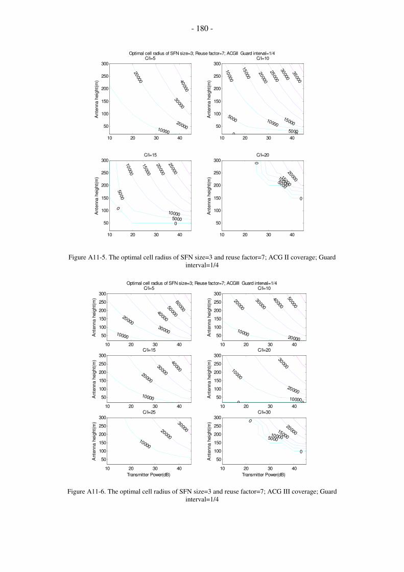
- 180 -

10 20 30 40

50

100

150

200

250

300

Ante

nna h

eig

ht(

m)

C/I=5

10000

20000

20000

3000040

000

10 20 30 40

50

100

150

200

250

300

Ante

nna h

eig

ht(

m)

C/I=10

0 0

5000

5000

1000

0

10000

15000

15000

20000

25000

30000

35000

10 20 30 40

50

100

150

200

250

300

Ante

nna h

eig

ht(

m)

C/I=15

0

0

5000

5000

10

000

10000

15000

20000

25000


10 20 30 40

50

100

150

200

250

300

Ante

nna h

eig

ht(

m)

C/I=20

0

0

5000

10000

1500020000


interval=1/4

10 20 30 40

50

100

150

200

250

300

Ante

nna h

eig

ht(

m)

C/I=5

10000

2000030000

40000

5000060000

10 20 30 40

50

100

150

200

250

300

Ante

nna h

eig

ht(

m)

C/I=10

10000

20000

20000

30000

40000

50000

10 20 30 40

50

100

150

200

250

300

Ante

nna h

eig

ht(

m)

C/I=15

10000

20000

30000

40000

10 20 30 40

50

100

150

200

250

300

Ante

nna h

eig

ht(

m)

C/I=20

0 0

10000

10000

20000

30000

10 20 30 40

50

100

150

200

250

300


Ante

nna h

eig

ht(

m)

C/I=25

10000

20000

30000


10 20 30 40

50

100

150

200

250

300


Ante

nna h

eig

ht(

m)

C/I=30

0

0

500010000

15000

20000


interval=1/4

- 181 -

10 20 30 40

50

100

150

200

250

300

Ante

nna h

eig

ht(

m)

C/I=5

5000

10000

10000

15000

15000

20000

25000

30000

35000

10 20 30 40

50

100

150

200

250

300

Ante

nna h

eig

ht(

m)

C/I=10

10000

10000

20000

30000

10 20 30 40

50

100

150

200

250

300

Ante

nna h

eig

ht(

m)

C/I=15

0

0

50

00

5000

10000

15000

20000


10 20 30 40

50

100

150

200

250

300

Ante

nna h

eig

ht(

m)

C/I=20

0

5000

10000

15000


interval=1/4

10 20 30 40

50

100

150

200

250

300

Ante

nna h

eig

ht(

m)

C/I=5

10000

20000

30000

40000

10 20 30 40

50

100

150

200

250

300

Ante

nna h

eig

ht(

m)

C/I=10

5000

10000

10000

15000

20000

25000

30000

10 20 30 40

50

100

150

200

250

300

Ante

nna h

eig

ht(

m)

C/I=15

10000 20000

10 20 30 40

50

100

150

200

250

300

Ante

nna h

eig

ht(

m)

C/I=20

0

0500010000

15000

20000


10 20 30 40

50

100

150

200

250

300


Ante

nna h

eig

ht(

m)

C/I=25

05000

1000015000


interval=1/4

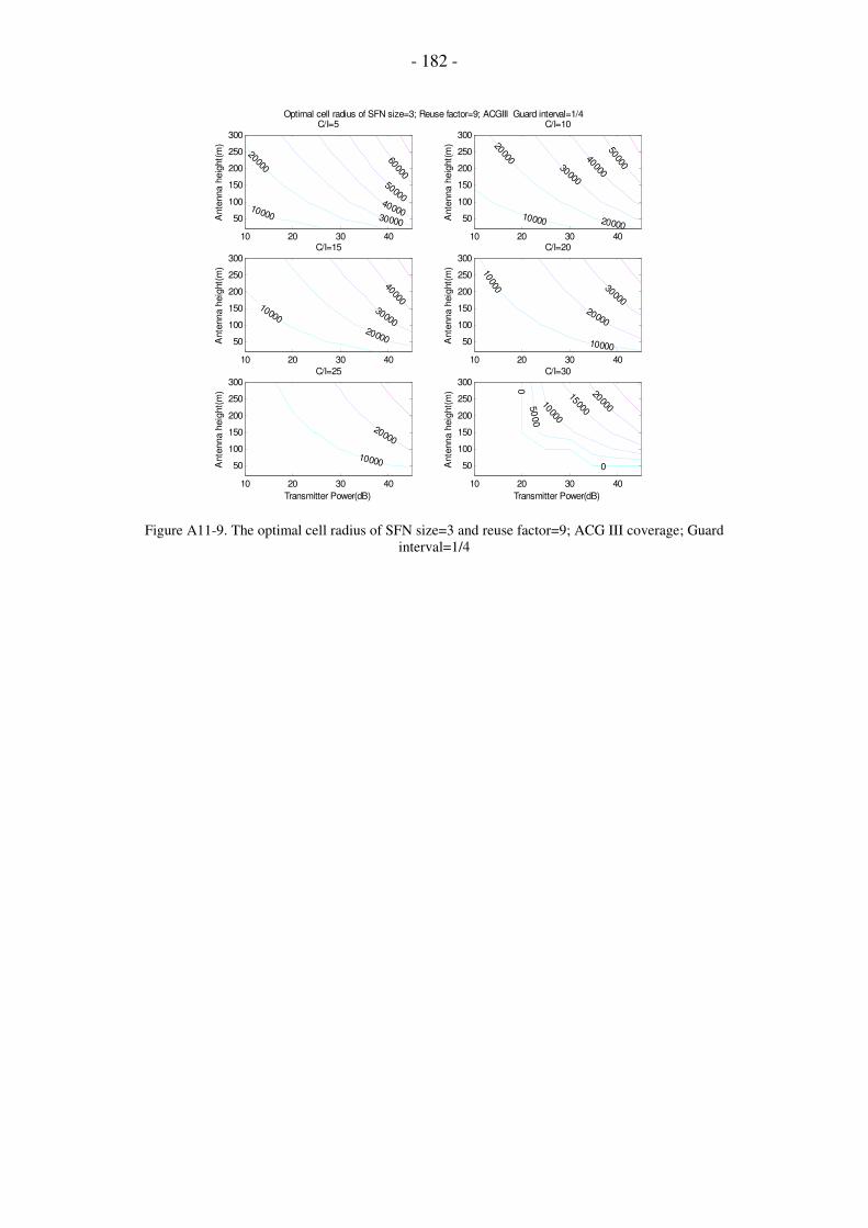
- 182 -

10 20 30 40

50

100

150

200

250

300

Ante

nna h

eig

ht(

m)

C/I=5

10000

20000

30000

40000

50000

60000

10 20 30 40

50

100

150

200

250

300

Ante

nna h

eig

ht(

m)

C/I=10

10000

20000

20000

30000

4000050000

10 20 30 40

50

100

150

200

250

300

Ante

nna h

eig

ht(

m)

C/I=15

10000

20000

30000

40000

10 20 30 40

50

100

150

200

250

300

Ante

nna h

eig

ht(

m)

C/I=20

10000

10000

20000

30000

10 20 30 40

50

100

150

200

250

300


Ante

nna h

eig

ht(

m)

C/I=25

10000

20000


10 20 30 40

50

100

150

200

250

300


Ante

nna h

eig

ht(

m)

C/I=30

0

0

50

00

10000

1500020000


interval=1/4

- 183 -

A12. The SFN gain for SFN size = 3 with reuse factor, guard interval=1/4;

10 15 20 25 30 35 40 45

50

100

150

200

250

300A

nte

nna h

eig

ht(

m)

C/I=5

0.1

0.1

0.1

0.20.2

0.20.3 0.3 0.30.40.40.4 0.50.50.6 0.60.7 0.8 0.9

10 15 20 25 30 35 40 45

50

100

150

200

250

300

Ante

nna h

eig

ht(

m)

C/I=10

0.5 0.50.5

0.5 0.5 0.5

111.5

SFN Gain of size=3 Reuse factor=3; ACGIII Guard interval=1/4

10 15 20 25 30 35 40 45

50

100

150

200

250

300

Ante

nna h

eig

ht(

m)

C/I=15

0.1

0.1 0.1

0.2

0.2 0.2

0.2 0.20.3

0.3 0.3

0.30.3

0.4

0.40.4

0.40.4

0.50.5

0.50.60.6

0.70.8

Figure A12-1. The SFN gain of a SFN size=3 and reuse factor=3; ACG III coverage; Guard

interval=1/4

10 15 20 25 30 35 40 45

50

100

150

200

250

300

Ante

nna h

eig

ht(

m)

C/I=5

0.2

0.2 0.2 0.2

0.2

0.20.2

0.4

0.4

0.40.6

0.811.2

SFN Gain of size=3 Reuse factor=7; ACGI Guard interval=1/4

10 15 20 25 30 35 40 45

50

100

150

200

250

300

Ante

nna h

eig

ht(

m)

C/I=10

0.050.10.15

Figure A12-2. The SFN gain of a SFN size=3 and reuse factor=7; ACG I coverage; Guard interval=1/4

- 184 -

10 15 20 25 30 35 40 45

50

100

150

200

250

300

Ante

nna h

eig

ht(

m)

C/I=5

0.1

0.1

0.1 0.1 0.1

0.2

0.20.2

0.2 0.2 0.2

0.3 0.3 0.3

0.3 0.3 0.30.4 0.4 0.40.4 0.4 0.40.50.5

10 15 20 25 30 35 40 45

50

100

150

200

250

300

Ante

nna h

eig

ht(

m)

C/I=10

0.1

0.1 0.1

0.10.

2

0.2 0.2

0.2

0.2

0.30.3

0.3

0.30.3

0.4

0.40.40.4

0.50.6

SFN Gain of size=3 Reuse factor=7; ACGII Guard interval=1/4

10 15 20 25 30 35 40 45

50

100

150

200

250

300

Ante

nna h

eig

ht(

m)

C/I=15

0.050.10.150.20.25

Figure A12-3. The SFN gain of a SFN size=3 and reuse factor=7; ACG II coverage; Guard

interval=1/4

10 20 30 40

50

100

150

200

250

300

Ante

nna h

eig

ht(

m)

C/I=5

0.05

0.1

0.10.15

0.210 20 30 40

50

100

150

200

250

300

Ante

nna h

eig

ht(

m)

C/I=10

0.05

0.1

0.10.15 0.150.2 0.20.25 0.250.30.35

10 20 30 40

50

100

150

200

250

300

Ante

nna h

eig

ht(

m)

C/I=15

0.05 0.05

0.1

0.1 0.1

0.1

5

0.15

0.15 0.15

0.20.2

0.2 0.2

0.250.25

0.250.3

10 20 30 40

50

100

150

200

250

300

Ante

nna h

eig

ht(

m)

C/I=20

0.1

0.1

0.1

0.2

0.2

0.20.30.

3

0.30.4

0.40.50.6


10 20 30 40

50

100

150

200

250

300


Ante

nna h

eig

ht(

m)

C/I=25

0.050.1

0.15

0.150.2

0.2

0.25 0.30.35


interval=1/4

- 185 -

10 15 20 25 30 35 40 45

50

100

150

200

250

300

Ante

nna h

eig

ht(

m)

C/I=5

0.5

0.5

1

1

1.5

2 2.5

SFN Gain of size=3 Reuse factor=9; ACGI Guard interval=1/4

10 15 20 25 30 35 40 45

50

100

150

200

250

300

Ante

nna h

eig

ht(

m)

C/I=10

0.1

0.1 0.1

0.10.2

0.2

0.2

0.2

0.3

0.3

0.3

0.4

Figure A12-5. The gain of a SFN size=3 and reuse factor=9; ACG I coverage; Guard interval=1/4

10 15 20 25 30 35 40 45

50

100

150

200

250

300

Ante

nna h

eig

ht(

m)

C/I=5

0.05 0.05 0.05

0.1

0.1

0.1 0.1 0.1

0.15

0.15

0.15

0.15 0.15 0.15

0.2 0.20.2

0.2 0.2 0.20.25 0.25 0.250.250.250.25

10 15 20 25 30 35 40 45

50

100

150

200

250

300

Ante

nna h

eig

ht(

m)

C/I=10

0.0

5

0.05 0.05 0.05

0.1

0.1 0.1 0.1

0.1

0.1

5

0.15 0.15 0.15

0.15

0.15

0.2

0.2 0.2 0.2

0.2

0.20.2

0.25

0.25 0.25

0.25

0.250.25 0.30.30.3

0.3 0.3

0.3

0.350.35

0.35 0.35 0.35

0.40.40.45

SFN Gain of size=3 Reuse factor=9; ACGII Guard interval=1/4

10 15 20 25 30 35 40 45

50

100

150

200

250

300

Ante

nna h

eig

ht(

m)

C/I=15

0.1

0.1

0.10.2

0.2

0.2

0.2

0.3

0.30.30.40.5

Figure A12-6. The gain of a SFN size=3 and reuse factor=9; ACG II coverage; Guard interval=1/4

- 186 -

10 20 30 40

50

100

150

200

250

300

Ante

nna h

eig

ht(

m)

C/I=5

0.040.06

0.0

8

0.08

0.1

0.10.12

0.120.140.14

0.160.1810 20 30 40

50

100

150

200

250

300

Ante

nna h

eig

ht(

m)

C/I=10

0.05

0.1

0.10.15 0.150.2 0.20.25

10 20 30 40

50

100

150

200

250

300

Ante

nna h

eig

ht(

m)

C/I=15

0.2 0.20.40.40.6 0.81

10 20 30 40

50

100

150

200

250

300

Ante

nna h

eig

ht(

m)

C/I=20

0. 1

0.1

0.1

0.2

0.20.2

0.20.3

0.3

0.30.4

0.4 0.50.5

0.6

10 20 30 40

50

100

150

200

250

300


Ante

nna h

eig

ht(

m)

C/I=25

0.1

0.1

0.2

0.2

0.3

0.3

0.4


10 20 30 40

50

100

150

200

250

300


Ante

nna h

eig

ht(

m)

C/I=30

Figure A12-7. The gain of a SFN size=3 and reuse factor=9; ACG III coverage; Guard interval=1/4

- 187 -

A13. The optimal cell radius of SFN size = 7 with a reuse factor, guard interval =

1/4

10 15 20 25 30 35 40 45

50

100

150

200

250

300

Ante

nna h

eig

ht(

m)

C/I=5

0 0 0 02000 2000 2000

6000

6000 6000

9000

9000

9000

12000

12000

12000

20000

20000

40000


10 15 20 25 30 35 40 45

50

100

150

200

250

300


Ante

nna h

eig

ht(

m)

C/I=10

0

0

0 0

2000

2000

2000

6000

60006000

9000

90009000

12000

12000

12000

20000

20000


interval=1/4

10 15 20 25 30 35 40 45

50

100

150

200

250

300

Ante

nna h

eig

ht(

m)

C/I=5

2000 6000

6000

90009000

900012000

1200012000

20000

20000

20000

40000

10 15 20 25 30 35 40 45

50

100

150

200

250

300

Ante

nna h

eig

ht(

m)

C/I=10

0 0 0 02000 2000 2000

6000

60006000

9000

9000

9000

12000

12000

12000

20000

20000

40000


10 15 20 25 30 35 40 45

50

100

150

200

250

300


Ante

nna h

eig

ht(

m)

C/I=15

0

0

0

2000

2000

2000

6000

6000

6000

9000

9000

9000

1200012000

20000

20000


interval=1/4

- 188 -

10 20 30 40

50

100

150

200

250

300

Ante

nna h

eig

ht(

m)

C/I=5

9000

12000

20000

40000

60000

10 20 30 40

50

100

150

200

250

300

Ante

nna h

eig

ht(

m)

C/I=10

60009000

12000

20000

20000

40000

10 20 30 40

50

100

150

200

250

300

Ante

nna h

eig

ht(

m)

C/I=15

20006000

9000

12000

12000

20000

40000

10 20 30 40

50

100

150

200

250

300

Ante

nna h

eig

ht(

m)

C/I=20

0 02000

2000

6000

6000

9000

9000

1200012000

20000

10 20 30 40

50

100

150

200

250

300


Ante

nna h

eig

ht(

m)

C/I=25

0

0

20

00

2000

60

00

6000

900012000

20000


10 20 30 40

50

100

150

200

250

300


Ante

nna h

eig

ht(

m)

C/I=30

0200060009000

12000


interval=1/4

10 20 30 40

50

100

150

200

250

300

Ante

nna h

eig

ht(

m)

C/I=5

6000

9000

12000

12000

20000

10 20 30 40

50

100

150

200

250

300

Ante

nna h

eig

ht(

m)

C/I=10

02000

6000

6000

9000

9000

12000

20000

10 20 30 40

50

100

150

200

250

300

Ante

nna h

eig

ht(

m)

C/I=15

00

2000

2000

6000

6000

9000

9000

12000

20000

10 20 30 40

50

100

150

200

250

300

Ante

nna h

eig

ht(

m)

C/I=20

0

0

2000

2000

6000

9000

12000


10 20 30 40

50

100

150

200

250

300


Ante

nna h

eig

ht(

m)

C/I=25

0200060009000


interval=1/4

- 189 -

10 20 30 40

50

100

150

200

250

300

Ante

nna h

eig

ht(

m)

C/I=5

60009000

12000

20000

40000

10 20 30 40

50

100

150

200

250

300

Ante

nna h

eig

ht(

m)

C/I=10

6000

9000

12000

12000

20000

10 20 30 40

50

100

150

200

250

300

Ante

nna h

eig

ht(

m)

C/I=15

02000

6000

6000

9000

9000

12000

20000

10 20 30 40

50

100

150

200

250

300

Ante

nna h

eig

ht(

m)

C/I=20

0

0

2000

200060

006000

9000

12000

20000

10 20 30 40

50

100

150

200

250

300


Ante

nna h

eig

ht(

m)

C/I=25

0

0200060009000

12000


10 20 30 40

50

100

150

200

250

300


Ante

nna h

eig

ht(

m)

C/I=30

020006000


interval=1/4

10 20 30 40

50

100

150

200

250

300

Ante

nna h

eig

ht(

m)

C/I=5

900012000

20000

40000

60000

10 20 30 40

50

100

150

200

250

300

Ante

nna h

eig

ht(

m)

C/I=10

60009000

12000

20000

20000

40000

10 20 30 40

50

100

150

200

250

300

Ante

nna h

eig

ht(

m)

C/I=15

6000

900012000

20000

40000

10 20 30 40

50

100

150

200

250

300

Ante

nna h

eig

ht(

m)

C/I=20

2000

60009000

900012000

12000

20000

10 20 30 40

50

100

150

200

250

300


Ante

nna h

eig

ht(

m)

C/I=25

0 02000

2000

6000

6000

9000

9000

12000

20000


10 20 30 40

50

100

150

200

250

300


Ante

nna h

eig

ht(

m)

C/I=30

0

0

20

00

2000

6000

6000

9000

12000

20000


interval=1/4

- 190 -

10 20 30 40

50

100

150

200

250

300

Ante

nna h

eig

ht(

m)

C/I=5

60009000

12000

12000

20000

10 20 30 40

50

100

150

200

250

300

Ante

nna h

eig

ht(

m)

C/I=10

2000

6000

9000

9000

12000

20000

10 20 30 40

50

100

150

200

250

300

Ante

nna h

eig

ht(

m)

C/I=15

0 0

20002000

6000

6000

9000

9000

12000

20000

10 20 30 40

50

100

150

200

250

300

Ante

nna h

eig

ht(

m)

C/I=20

0

0

2000

200060

006000

9000

12000


10 20 30 40

50

100

150

200

250

300


Ante

nna h

eig

ht(

m)

C/I=25

02000

6000 9000

12000


interval=1/4

10 20 30 40

50

100

150

200

250

300

Ante

nna h

eig

ht(

m)

C/I=5

6000 900012000

20000

40000

10 20 30 40

50

100

150

200

250

300

Ante

nna h

eig

ht(

m)

C/I=10

60009000

12000

12000

20000

10 20 30 40

50

100

150

200

250

300

Ante

nna h

eig

ht(

m)

C/I=15

2000 6000

6000

9000

9000

12000

20000

10 20 30 40

50

100

150

200

250

300

Ante

nna h

eig

ht(

m)

C/I=20

00

20002000

6000

6000

9000

12000

20000

10 20 30 40

50

100

150

200

250

300


Ante

nna h

eig

ht(

m)

C/I=25

0

0

2000

2000

6000

9000

12000


10 20 30 40

50

100

150

200

250

300


Ante

nna h

eig

ht(

m)

C/I=30

02000

60009000

12000


interval=1/4

- 191 -

10 20 30 40

50

100

150

200

250

300

Ante

nna h

eig

ht(

m)

C/I=5

6000 900012000

20000

40000

60000

10 20 30 40

50

100

150

200

250

300

Ante

nna h

eig

ht(

m)

C/I=10

6000

9000

12000

20000

40000

10 20 30 40

50

100

150

200

250

300

Ante

nna h

eig

ht(

m)

C/I=15

6000 900012000

20000

40000

10 20 30 40

50

100

150

200

250

300

Ante

nna h

eig

ht(

m)

C/I=20

6000 9000

9000

12000

1200020000

10 20 30 40

50

100

150

200

250

300


Ante

nna h

eig

ht(

m)

C/I=25

02000

6000

6000

9000

900012000

20000


10 20 30 40

50

100

150

200

250

300


Ante

nna h

eig

ht(

m)

C/I=30

0

0

2000

2000

6000

6000

9000

12000

20000


interval=1/4

- 192 -

A14. The SFN gain for SFN size = 7 with a reuse factor, guard interval=1/4

10 15 20 25 30 35 40 45

50

100

150

200

250

300

Ante

nna h

eig

ht(

m)

C/I=5;SFN Gain of SFN size=7 Reuse factor=3; ACGII Guard interval=1/4

0.1

0.2

0.30.40.50.6


interval=1/4

10 15 20 25 30 35 40 45

50

100

150

200

250

300

Ante

nna h

eig

ht(

m)

C/I=5

0.2 0.20.2

0.4 0.4 0.40.60.60.8 0.81

10 15 20 25 30 35 40 45

50

100

150

200

250

300

Ante

nna h

eig

ht(

m)

C/I=10

0.02

0.02 0.02

0.04

0.04 0.04

0.06

0.06 0.06

0.08

0.08 0.08

0.1

0.1 0.1

0.10.12

0.12 0.12

0.120.12

0.14

0.140.14

0.14

0.14

0.160.16

SFN Gain of SFN size=7 Reuse factor=3; ACGIII Guard interval=1/4

10 15 20 25 30 35 40 45

50

100

150

200

250

300


Ante

nna h

eig

ht(

m)

C/I=15

0.1

0.1 0.1

0.2

0.2 0.2

0.20.3

0.3 0.3

0.30.3

0.4

0.4

0.4

0.4 0.4

0.5

0.50.5 0.50.60.6

0.70.80.9


interval=1/4

- 193 -

10 15 20 25 30 35 40 45

50

100

150

200

250

300

Ante

nna h

eig

ht(

m)

C/I=5;SFN Gain of SFN size=7 Reuse factor=7; ACGI Guard interval=1/4

0.2

0.2

0.20.2

0.2

0.2

0.2

0.4

0.4

0.4

0.4

0.4

0.4

0.6

0.60.6

0.811.2

1.4 1.6


10 15 20 25 30 35 40 45

50

100

150

200

250

300

Ante

nna h

eig

ht(

m)

C/I=5

0.1 0.1 0.1

0.2

0.2

0.2 0.2 0.2

0.3

0.30.3

0.3 0.3 0.3

0.4 0.4 0.4

0.4 0.4 0.4

0.5 0.5 0.50.5 0.5 0.50.6

0.60.60.6 0.60.7

10 15 20 25 30 35 40 45

50

100

150

200

250

300

Ante

nna h

eig

ht(

m)

C/I=10

0.02 0.040.060.080.10.120.14

SFN Gain of SFN size=7 Reuse factor=7; ACGII Guard interval=1/4

10 15 20 25 30 35 40 45

50

100

150

200

250

300


Ante

nna h

eig

ht(

m)

C/I=15

0.05 0.10.150.20.250.3


interval=1/4

- 194 -

10 20 30 40

50

100

150

200

250

300

Ante

nna h

eig

ht(

m)

C/I=5

0.05

0.1

0.1

0.15

0.150.20.20.250.3

10 20 30 40

50

100

150

200

250

300

Ante

nna h

eig

ht(

m)

C/I=10

0.05

0.05

0.1

0.1 0.1

0.15

0.150.15

0.20.2

10 20 30 40

50

100

150

200

250

300

Ante

nna h

eig

ht(

m)

C/I=15

0.05 0.05

0.1

0.1 0.1

0.15

0.15 0.15

0.2

0.2

0.2 0.2

0.25

0.25

0.25 0.25

0.3 0.30.3 0.30.35 0.35

10 20 30 40

50

100

150

200

250

300

Ante

nna h

eig

ht(

m)

C/I=20

0.1

0.1

0.1

0. 2

0.2

0.20.3

0.3

0.30.40.

4

0.4

0.50.60.7


10 20 30 40

50

100

150

200

250

300


Ante

nna h

eig

ht(

m)

C/I=25

0.050.10.15

0.150.2

0.2

0.250.30.35


interval=1/4

10 15 20 25 30 35 40 45

50

100

150

200

250

300

Ante

nna h

eig

ht(

m)

C/I=5;SFN Gain of SFN size=7 Reuse factor=9; ACGI Guard interval=1/4

0.5

0.5

0.5

0.51

1

1.5

1.5

2

2

2.5

3


- 195 -

10 15 20 25 30 35 40 45

50

100

150

200

250

300

Ante

nna h

eig

ht(

m)

C/I=5

0.05 0.05 0.050.1 0.1 0.1

0.15

0.15

0.15 0.15 0.15

0.2

0.2

0.2

0.2 0.2 0.2

0.25

0.250.25

0.25 0.25 0.25

0.3

0.30.3

0.30.3 0.3 0.3

0.35 0.350.350.35 0.35 0.35

0.40.4 0.40.40.4

10 15 20 25 30 35 40 45

50

100

150

200

250

300

Ante

nna h

eig

ht(

m)

C/I=10

0.05

0.05

0.1

0.1

0.15

0.15

0.15

0.2

SFN Gain of SFN size=7 Reuse factor=9; ACGII Guard interval=1/4

10 15 20 25 30 35 40 45

50

100

150

200

250

300


Ante

nna h

eig

ht(

m)

C/I=15

0.1

0.1

0.2

0.2

0.20.3 0.3

0.30.30.4

0.40.5 0.6


interval=1/4

10 20 30 40

50

100

150

200

250

300

Ante

nna h

eig

ht(

m)

C/I=5

0.05

0.1

0.10.15

0.150.2 0.2510 20 30 40

50

100

150

200

250

300

Ante

nna h

eig

ht(

m)

C/I=10

0.05

0.1

0.15

0.150.2

0.20.25 0.250.30.35

10 20 30 40

50

100

150

200

250

300

Ante

nna h

eig

ht(

m)

C/I=15

0.2

0.2

0.4 0.40.6 0.60.81 1.210 20 30 40

50

100

150

200

250

300

Ante

nna h

eig

ht(

m)

C/I=20

0.1

0.1

0.1

0.2

0.2

0.2

0.3

0.3

0.3

0.30.4

0.40.5

0.5 0.60.6 0.70.7 0.8

10 20 30 40

50

100

150

200

250

300


Ante

nna h

eig

ht(

m)

C/I=25

0.1

0.1

0.2

0.2

0.3

0.3

0.30.4

0.5


10 20 30 40

50

100

150

200

250

300


Ante

nna h

eig

ht(

m)

C/I=30


interval=1/4

deliverable 6 - brunel university london

Documents