deformation monitoring
TRANSCRIPT

OPTIMIZATION AND DESIGNOF DEFORMATION
MONITORING SCHEMES
KUANG SHAN-LONG
September 1991
TECHNICAL REPORT NO. 157

PREFACE
In order to make our extensive series of technical reports more readily available, we have scanned the old master copies and produced electronic versions in Portable Document Format. The quality of the images varies depending on the quality of the originals. The images have not been converted to searchable text.

OPTIMIZATION AND DESIGN OF DEFORMATION MONITORING SCHEMES
Kuang Shan-long
Department of Geodesy and Geomatics Engineering University of New Brunswick
P.O. Box 4400 Fredericton, N .B.
Canada E3B 5A3
September 1991 Latest Reprinting December 1994
© Kuang Shan-long, 1991

PREFACE
This technical report is a reproduction of a dissertation submitted in partial fulfillment of
the requirements for the degree of Doctor of Philosophy in the Department of Surveying
Engineering, July 1991. The research was supervised by Dr. Adam Chrzanowski, and
funding was provided partially by the Natural Sciences and Engineering Research Council
of Canada and by the University of New Brunswick.
As with any copyrighted material, permission to reprint or quote extensively from this
report must be received from the author. The citation to this work should appear as
follows:
Kuang, Shan-long (1991). Optimization and Design of Deformation Monitoring Schemes. Ph.D. dissertation, Department of Surveying Engineering Technical Report No. 157, University of New Brunswick, Fredericton, New Brunswick, Canada, 179 pp.

ABSTRACT
A methodology for the optimization and design of integrated deformation
monitoring schemes has been developed in this research. Examples with real and
simulated data are given which demonstrate the usefulness of the newly developed
methodology. It is now possible to design integrated deformation monitoring schemes
with any type of geodetic and geotechnical observations scattered in space and time
to monitor any type of deformations. The methodology includes all the intentions of the
conventional First Order, Second Order and Third Order Designs of geodetic networks
by allowing for separate or simultaneous optimization of the geometrical
configuration and weights of heterogeneous observables of a monitoring scheme
analyticallv. It allows for a simultaneous consideration of all the quality aspects, i.e.
precision, internal and/or external reliability, sensitivity and economy of a monitoring
scheme. The developed methodology can be used for the optimal design of either one-,
two-, or three-dimensional monitoring schemes. An extension of its application to the
optimal design of any geodetic networks for engineering purposes is quite straight
forward.
ii

TABLE OF CONTENTS
Page
ABSTRACT . . . . . . . . . . . . . . . . . . . . . . . . . . . . . . . . . . . . . . . . . . . . . . . . . . . . .. . . . . . . . . . . . . . . . . . . . . . . . . . n
LIST OF TABLES
LIST OF FIGURES
. . . . . . . . . . . . . . . . . . . . . . . . . . . . . . . . . . . . . . . . . . . . . . . . . . . . . . . . . . . . . . . . . . . . . . . . v
• • • • • • • • • • • • • • • • • • • • • • • • • • • • • • • • • • • • • • • • • • • • • • • • • . • • • • • • • • • • • • • • • • • • V1l
ACKNO~DGEMENTS Vlll
1.
2.
3.
INTRODUCTION 1
1. 1 The Motive . . . . . . . . . . . . . . . . . . . . . . . . . . . . . . . . . . . . . . . . . . . . . . . . . . . . . . . . . . . . . . . . 1 1.2 Identification of Problems and Scope of the Thesis ... ..... ....... ... 4 1. 3 Organization of the Contents and Summary
of the Contributions . . . . . . . . . . . . . . . . . . . . . . . . . . . . . . . . . . . . . . . . . . . . . . . . . . . . . 14
DEFORMATION MONITORING AND TilE DESIGN PROBLEM 17
2.1 Basic Deformation Parameters and the Deformation Models . . . . . . . . . . . . . . . . . . . . . . . . . . . . . . . . . . . . . . . . . . . . . . . . . . . 17
2.2 Geodetic and Non-geodetic Methods for Deformation Monitoring . . . . . . . . . . . . . . . . . . . . . . . . . . . . . . . . . . . . . . . . . . . 21
2. 3 Estimation of Deformation Models and the Design Problem .. . . . .. . . . . . . . . . . . . . . . . . . . . . . . . . . . . . .. . . . . .. . . . . 29 2.3.1 The functional relationship between
the deformation models and the observed quantities .. . . . .. ... . . . . . .. . . . . . . . . . . . . . . .. . . . . . . . . . . . . 29
2. 3. 2 Estimation of deformation parameters and the design problem . .. .. . .. . .. .. .. .. .. .. .. .. .. .. . .. .. .. .. .. 31
QUALITY CONTROL MEASURES AND OPTIMALITY CRITERIA FOR DEFORMATION MONITORING SCHEMES 34
3.1 Measures and Criteria for Precision .................................. 35 3.1.1 Scalar precision functions .................................. ...... 35 3.1.2 Criterion matrices .................................................. 37 3 .1. 3 The datum problem for criterion matrices . . . . . . . . . . . . . . . . . . . 48
3.2 Measures and Criteria for Reliability .................................. 49 3.2.1 Gross errors and hypothesis testing ............................ 50 3.2.2 Reliability measures ............................................ 55 3. 2. 3 The optimality criteria . .. . .. . .. .. . .. .. . .. .. .. .. . .. .. .. .. .. .. .. .. 57
3.3 Measures and Criteria for Sensitivity ................................. 59 3.4 Measures and Criteria for Economy .. . .. .. .. .. .. .. .. .. .. .. .. .. .. . .. .. . 64
iii

TABLE OF CONTENTS (Cont'd) Page
4. OIYI1MIZATION ANDDESIGNOFDEFORMATION MONITORING SCHEMES .................................................. 66
4.1 Design Orders of a Monitoring Scheme .............................. 66 4.2 Identification of Unknown Parameters
to Be Optinlized . . . . . . . . . . . . . . . . . . . . . . . . . . . . . . . . . . . . . . . . . . . . . . . . . . . . . . . . . 68 4.3 Basic Requirements for An Optimal
Monitoring Scheme . . . . . . . . . . . . . . . . . . . . . . . . . . . . . . . . . . . . . . . . . . . . . . . . . . . . . 71 4.3.1 Precision requirement . . . . . .. . . . . . . . . . . . . . . . . . . . . . . . . . . . . . . . . . . . 72 4.3.2 Internal reliability requirement ........................ .... .... 78 4.3.3 External reliability requirement ... . .. . .. . . . ... . ... .. ... ... .... 82 4.3.4 Sensitivity requirement ... .... .. . . . . . . . ... . . . .. . . .. .. .. . .. . .. .. 84 4.3.5 Costrequirement ............................................... 85 4.3.6 Physical constraints ..... ... . . . . . . . .. . . . . .. .. .. . . . . . . . . .. . .. .. . . 86
4. 4 Formulation of Mathematical Models for Optinlization . . . . . . . . . . . . . . . . . . . . . . . . . . . . . . . . . . . . . . . . . . . . . . . . . . . . . . . . . 88
4. 5 Solution of the Mathematical Models . . . . . . . . . . . . . . . . . . . . . . . . . . . . . . . . . 92 4.5.1 The choice of norm ......... ...... ... .......................... 92 4.5.2 The solution methods ................ ... ....................... 96
4.6 Analysis of Solvability and the Multi-Objective Optimization Model (MOOM) . . . . . . . . . . . . . . . . . . . . . . . . . . 97 4.6.1 The concept of multi-objective optimization .................... 97 4.6.2 The Multi-Objective Optimization Model (MOOM)
for monitoring schemes . .. . .. .. . . . . . . . . .. .. . .. .. . . . . . . . .. . .. .. . . . 100 4. 7 Summary of the Optimization Procedures .............. ............... .. 104
5. SIMULATION STUDIES AND OPTIMIZATION EXAMPLES .......... 107
6.
5. 1 Simulation Studies . . . . . . . . . . . . . . . . . . . . . . . . . . . . . . . . . . . . . . . . . . . . . . . . . . . . . . 107 5 .1.1 Simulation study No. 1: Verification of the
correctness of the developed mathematical models . . ... .. . .. . . . 107 5 .1. 2 Simulation study No. 2: Influence of the position
changes on the solution of observation weights ............... 118 5.2 Optimization Examples ............................................... ..... 126
5.2.1 Example No. 1: Optimal design of a monitoring network - comparison of different approaches ................. 126
5.2.2 Example No.2: Optimization of the Mactaquac monitoring network . . . . . . . . . . . . . . . . . . . . . . . . . . . . . . . . . . . . . . . . . . . 140
SUMMARY OF RESULTS AND CONCLUSIONS
REFERENCES
160
166
175
177
APPENDIX I
APPENDIX II
IV

LIST OF TABLES
2.1 The geodetic methods for deformation monitoring . . . . . . . . . . . . . . . . . . . . . . . 25
2.2 The Non-Geodetic methods for deformation monitoring . . . . . . . . . . . . . . . . . . . . . . . . . . . . . . . . . . . . . . . . . . . . . . . . . . . . . . . . . . . . . . . . . . . . . 26
3.1 Lower bounds Bo for noncentrality parameter in dependency of the significance number a and the
required minimum power 1-13 of the test . . . . . . . . . . . . . . . . . . . . . . . . . . . . . . . . . . . 55
5.1 Desired coordinates for the geodetic netpoints 108
5.2 The input approximate coordinates of geodetic netpoints . . . . . . . . . . . . . . .. . . . . . . . . . . . . . . . . . .. . . . . . . . . . . . . .. . . . . . . . . . . . . . . . . . . . . 113
5.3 Comparison between the simulated position shifts and the optimized position corrections . . . . . . . . . . . . . . . . . . . . . . . . . . . . . . . . . . . 113
5.4 Comparison between the simulated weights and the optimized weights . . . . . . . . . . . . . . . . . . . . . . . . . . . . . . . . . . . . . . . . . . . . . . . . . . . . . . 114
5.5 Comparison between the simulated standard
5.6
5.7
deviations and the optimized values ....................................... 115
Goodness of fitting of the internal reliability 116
Goodness of fitting of external reliability 117
5.8 Desired coordinates for the three-D geodetic network . . . . . . . . . . . . . . . . . . . . . . . . . . . . . . . . . . . . . . . . . . . . . . . . . . . . . . . . . . . . . . . . . . . . . . . 122
5.9 The input approximate coordinates for the three-D. geodetic network . . . . . . . . . . . . . . . . . . . . . . . . . . . . . . . . . . . . . . . . . . . . . . . . . . . . . . . . . . . . . 122
5.10 Comparison between the simulated position shifts and the optimized position corrections ... .. .. .. .... ...... ...... .. . ..... ........ 123
5.11 Comparison between the simulated weights and the optimized weights . . . . . . . . . . . . . . . . . . . . . . . . . . . . . . . . . . . . . . . . . . . . . . . . . . . . . . . . . 124
. . .... ,..._.'
5.12 Comparison between the simulated weights and the optimized weights(SOD only) ......................................... 125
5.13 The approximate coordinates of the monitoring network ............................ ................................. .......... 127
5.14 Goodness of fitting of the precision criteria 133
v

5.15 The desired weights of the observations obtained by different approaches . . . . . . . . . . . . . . . . . . . . . . . . . . . . . . . . . . . . . . . . . . . . . . . . . . . . . 134
5.16 Possible coordinate shifts of netpoints and actual coordinate shifts resulting from the optimization
5.17 Goodness of fitting of the precision criteria with the input
135
approximate weights of observations changed . . . . . . . . . . . . . . . . . . . . . . . . . . 136
5.18 The desired weights of observations with the input approximate weights of observations changed
5.19 Possible coordinate shifts and actual coordinate shifts with the input approximate weights of
137
observations changed ....................................................... 138
5.20 Results of Method IV when the maximum
5.21
5.22
5.23
5.24
5.25
possible position shifts can be up to± 400 meters ..................... 139
The approximate coordinates of the Mactaquac monitoring network ........................................................ .
Station 95.000 % confidence ellipses for the original observation scheme (Factor used for obtaining these ellipses from standard error ellipses =2.4484)
Station 95.000 % confidence ellipses after deleting 31 distances (Factor used for obtaining these ellipses from standard error ellipses =2.4484) ................................... .
Station 95 % confidence ellipses for the optimized observation scheme ( Factor used for obtaining these ellipses from standard error ellipses=2.4484) .................................... .
Station 95.000% confidence ellipses for the optimized observation scheme (aim at improving accuracies of object points only, factor used for obtaining these ellipses from standard error ellipses =2.4484) ................................... .
vi
144
145
146
147
148

LIST OF FIGURES
Figure
2.1 Typical deformation models . . . . . . . . . . . . . . . . . . . . . . . . . . . . . . . . . . . . . . . . . . . . . . . . 21
2.2 A Reference Monitoring Network . . . . . . . . . . . . . . . . . . . . . . . . . . . . . . . . . . . . . . . . . . 24
2.3 A Relative Monitoring Network . . . . . . . . . . . . . . . . . . . . . . . . . . . . . . . . . . . . . . . . . . . . 24
3.1 Density functions of test statistic w i . . . . . . . . . . . . . . . . . . . . . . . . . . . . . . . . . . . . . . . . 53
4.1 A deformation monitoring scheme .. . .. .... ... .... .. . .. . .. . .. ...... ... . . . . .. 69
4.2 Diagram of the computation procedure for the optimization of monitoring schemes . . . . . . . . . . . . . . . . . . . . . . . . . . . . . . . . . . . . . . . . . . . . . . . . . . . . . . . . 106
5.1
5.2
5.3
5.4
The simulated monitoring scheme
The simulated 3-D geodetic network
The monitoring network
Layout of the Mactaquac Generating Station
5.5 Mactaquac Monitoring Net-- the observable
108
118
127
149
distances(Total: 176 distances) . . . . . . . . . . . . . . . . . . . . . . . . . . . . . . . . . . . . . . . . . . . . 150
5.6 Mactaquac Monitoring Net-- the deleted distances by optimization (Total: 31)
5.7 Mactaquac Monitoring Net-- the optimized
151
trilateration . . . . . . . . . . . . . . . . . . . . . . . . . . . . . . . . . . . . . . . . . . . . . . . . . . . . . . . . . . . . . . . . . . . 152
5.8 Mactaquac Monitoring Net-- the observable directions (Total: 352 directions) .. . . . . . . . . . . . . .. . . . . . . .. . . . . . . . . . . . . . .. . . . 153
5.9
5.10
5.11
5.12
5.13
Mactaquac Monitoring Net-- the proposed directions by optimization (Total: 88)
95% Error Ellipses -- the original observation scheme
95% Error Ellipses-- after deleting 31 distances
95% Error Ellipses-- the optimized observation scheme
Mactaquac Monitoring Net -- the proposed directions by optimization (Total: 36)
154
155
156
157
158
5.14 95% Error Ellipses -- the optimized observation scheme ................... 159
vu

ACKNOWLEDGEMENTS
Great appreciation is due to organizations and individuals whose contribution was
instrumental in rendering the completion of this research work.
The financial support from the University of New Brunswick and the Natural
Science and Engineering Research Council of Canada is greatly appreciated.
I am very grateful to my supervisor, Dr. Adam Chrzanowski, for his continuous
assistance, guidance, and interest in this work. Our discussions _were always fruitful and
constructive.
I thank Dr. A. Kleusberg of the Department of Surveying Engineering at UNB, Dr.
B. G. Nickerson of the School of Computer Science at UNB, and Dr. W. R. Knight of the
Department of Mathematics and Statistics at UNB, for their many hours in reviewing the
original manuscript and for their valued comments. A special thanks goes to Dr. B.
Schaffrin of the Department of Geodetic Science and surveying at the Ohio State
University, my external examiner, for his constructive criticisms and suggestions.
Appreciation is also due to Dr. Y.Q. Chen of the Department of Engineering Surveying at
Wuhan Technical University of Surveying and Mapping for his valued comments on the
draft manuscript.
I wish to acknowledge my great appreciation to the Chairman of the Surveying
Engineering Department, the Secretaries, and all Faculty members for their assistance and
support which have contributed in one way or another towards the successful completion
viii

of this research. Mr. James Secord is especially thanked for providing a data file of the
Mactaquac monitoring network.
I also wish to thank my graduate colleagues in the Department of Surveying
Engineering for their good company and encouragement. In particular, I wish to mention
Maenda Kwimbere, Edward Light, James Olaleye, Ogundare John, and Abidin Hasan.
Working and studying with them was a pleasure and an education. Mr. Edward Light also
did part of the proofreading.
Finally, to my wife Xiping, whose support and encouragement have never wavered
in my life, I express my deepest thanks.
lX

CHAPTER 1
INTRODUCTION
1.1 The Motive
Deformation refers to the changes a deformable body undergoes in its shape,
dimension, and position. It can be said that any object, natural or man-made, undergoes
changes in space and time. The determination and interpretation of the changes are the main
goal of deformation surveys.
Deformation surveys are one of the most important activities in surveying,
especially in engineering surveying. Their results are directly relevant to the safety of
human life and engineering structures. Deformation surveys can provide not only the
geometric status of the deformed object, but also information on its response to loading
stress. This provides a better understanding of the mechanics of deformations and the
checking of various theoretical hypotheses on the behavior of a deformable body.
Examples of deformation surveys include the monitoring of ground deformations due to
mining exploitation, withdrawal of oil or underground water, or construction of large
reservoirs; the monitoring of accumulation of stress near active tectonic plate boundaries;
and the checking of the stability of large or complex structures (e.g. hydro-electric dams).
As in conventional measurement, deformation measurements are undenaken in
three phases (Chen et al., 1983):
(i) Design of the surveying scheme;
(ii) The field observation campaign, and
1

(iii) Post-analysis of the data.
In the last few years, a considerable effort has been made to develop new
methodologies and new instrumentation for deformation monitoring, and for the post-
analysis of the data. Very little effort, however, was paid to developing methodologies for
the optimization and design of monitoring schemes with geodetic and non-geodetic
observables, as reflected in Chen (1983):
" ... A look at the research activities in the surveying community reveals that optimization and design of monitoring schemes with geodetic and non-geodetic observables require further research, especially in engineering surveys where the design problem is complicated ... "
The problem of the optimization and design of monitoring schemes has been recognized by
and incorporated into the study program of the international "ad hoc" Committee (FIG
Commission 6) on deformation analysis. The Department of Surveying Engineering at the
University of New Brunswick (UNB), referred to as the "Fredericton Group", is a member
of the FIG "ad hoc" Committee. Research Projects have been set up for the (Chrzanowski
and Secord, 1983):
(i) Optimization and design of monitoring networks with geodetic and non-
geodetic observables;
(ii) Evaluation of the observation data (including correlation of observations),
detection of outliers, and systematic errors;
(iii) Geometrical analysis of deformations;
(iv) Physical interpretation of deformations.
For a number of years, the Fredericton Group at UNB has been involved in the
development of new deformation surveying techniques and new methods for the post
analysis of deformation surveys. Since the "UN B Generalized Approach" for
deformation analysis was developed (Chrzanowski et al., 1982; Chen 1983), it has been
successfully applied in practice to a number of engineering and scientific projects.
2

Generally, this approach involves evaluation of the observation data; preliminary
identification of the deformation models; estimation of the deformation parameters; and
diagnostic checking of the models and the final selection of the "best" model. To ensure an
efficient implementation of the "UNB Generalized Approach", the optimization and
design of the monitoring scheme should precede the field observation and analysis
procedures. The optimization and design of a monitoring scheme are mainly comprised of:
(i) The determination of the required monitoring accuracy;
(ii) The selection of a monitoring methodology;
(iii) The determination of the optimal distribution of control and object points; and
(iv) The computation of the optimal distribution of required observational
accuracies among heterogeneous observables.
An optimized monitoring scheme will ensure the most economic field campaign, and it will
help in identifying, eliminating, or minimizing the effects of the gross and systematic errors
existing in the observation data prior to the estimation of deformation parameters in order to
avoid misinterpreting measuring errors as deformation phenomena. An optimized
monitoring scheme will also ensure the detection of predicted deformations according to a
selected tolerance criterion.
From the point of view of deformation mechanics, the state of a deformable body
may be either static, or kinematic, or dynamic. The design of a monitoring scheme depends
on the type, the magnitude, and the rate of the deformation. Compared with the design of
geodetic positioning surveys, the design of an integrated monitoring scheme with geodetic
. and non-geodetic instrumentation is much more complicated. The accuracy criterion, and
the plan of the "configuration", all require specialized treatment. Although optimization of
geodetic positioning networks has been extensively discussed, no previous work has been
done towards the optimization and design of integrated monitoring schemes with geodetic
and non-geodetic observables. It is for these reasons that this research was intended
3

to develop a methodoloev for the optimization and desien of inteerated
mQnitorine schemes with eeodetic and non-eeodetic observables.
1.2 Identification of Problems and Scope of the Thesis
In the past years, an abundance of papers appeared concerning the optimal design
of terrestrial geodetic networks, but very few have dealt specifically with deformation
monitoring schemes. While the usual geodetic surveys are concerned, in a static sense,
with determination of relative positions, a deformation monitoring scheme must be
considered as being changeable, either dynamically or kinematical! y, in space and time.
Thus the design of a monitoring scheme is concerned only with these changes e.g.
displacements or certain deformation parameters, depending on the attributes of the specific
problem. Niemeier ( 1981) proposed to optimize the configuration of levelling nets
according to the precision criteria set for deformation parameters representing crust
movements. Chen, et al. (1983) gave an example of optimizing the distribution of
observation weights based on the desired accuracy of strain parameters.
In principle, the optimization and design of a monitoring scheme can be approached
using basically the same philosophy as used in the optimal design of geodetic networks. In
the following, a review of the presently available methods, including both the criterion set
up and the solution methodology, is given first. Then the existing problems and the scope
of the thesis are clarified.
Grafarend (1974) classifies the geodetic network design by order, i.e.
Zero Order(WD): Design of reference system
First Order(FOD): Design of the network configuration
Second Order(SOD): Selection of the Observation weights
Third Order(IHOD): Addition of observations to improve the existing network
4

To the above design problems a fifth one can be added, called the Combined Design
(COMD) (Vanicek and Krakiwsky, 1986) problem, where both the First- and Second
Order Design problems have to be optimally solved simultaneously with a preassigned
covariance matrix of the parameters. A network should be designed in such a way that:
(1) The postulated precision of the network elements, and of arbitrary estimable
quantities, can be realized;
(2) It is as sensitive as possible to statistical testing procedures, which allow for
example the detection of outliers in the measurements;
(3) The marking of the points and the performance of the measurements are
satisfying some cost criteria.
The starting point of analytical optimization techniques with regard to geodetic
measurements was due to the dissertation of Helmert (1868), entitled "Studien tiber
rationelle Vermessungen im Gebiet der hoheren Geoda.sie". Since that time several of the
most exceptional geodesists have contributed to this subject, e.g. Schreiber(1882},
Jung(1924), and Wolf (1961). They all attempted to minimize some objective function
which describes the cost, precision, or reliability within a geodetic project by a scalar value.
Baarda (1962) proposed a completely different concept which dealt with a so-called
criterion matrix to be best approximated by the -actual covariance matrix of the estimated
parameters. These criterion matrices possess "ideal" structure (in a certain sense) which has
to be specified in each case. Grafarend (1972) introduced the Taylor-Karman structured
idealized variance-covariance matrix of Cartesian coordinates in two- and three-dimensional
geodetic networks based on the theory of turbulence. In Grafarend and Schaffrin( 1979),
TK-structures were studied generally with variance matrices for azimuths, angles and
distances derived from general and special dispersion matrices of Cartesian coordinates and
coordinate differences. In a subsequent publication, Schaffrin and Grafarend (1981) dealt
with the problem of allocated criterion matrices which were computed using generalized
5

inverses from the idealized variance-covariance matrix of azimuths, angles or distances
constructed under the postulate of homogeneity and isotropy. Molenaar(1981) extended the
two dimensional concept of Baarda into three dimensions by using quaternion algebra and
spherical coordinates.
The problem with the Taylor-Karman structured criterion matrices is· that the
requirement for statistical homogeneity and isotropy is too strict for real networks;
unrealistic requirements may lead to absurd design.
The solution strategies of the optimization problems in the different orders of the
design are dependent both on the mathematical form to which the problem has been
brought, and on the shape of the objective function which is representing the aim of the
design. Unfortunately, purely analytical solutions are known mainly in the second order
design, where the standard problems can be expressed in terms of linear equations and
linear inequalities.
A primitive method which is suited for FOD, SOD, and TROD is the computer
simulation, or "trial and error" method. In this method, a solution to the design problem is
postulated and the design and cost criteria computed. Should either of these criteria not be
fulfilled, a new solution is postulated (usually by slightly altering the original postulate) and
the criteria are recomputed. The procedure is repeated until a satisfactory (unlikely to be the
optimum) network is found. The process is summarized in more detail by the following
steps (Cross, 1985):
(i) specify precision and reliability criteria;
(ii) select an observation scheme (stations, observations, and weights);
(iii) Compute the covariance matrices of the desired least squares estimates and
derive the values of the quantities specified as precision and reliability criteria;
(iv) if these values are close to those specified in (i) then go to the next stage;
otherwise alter the observation scheme (by removing observations or
6

decreasing weights if the selected network is too good, or by adding
observations or increasing weights if it is not good enough) and return to (iii);
(v) compute the cost of the network and consider the possibility of returning to
(ii) and restarting the process with a completely different type of network
(e.g. a traverse instead of triangulation). Stop when it is believed that the
optimum (minimum cost) network has been found.
The method has been used for about twenty years now and is well established.
Some descriptions of software include Mepham (1983), Cross(1981), and Frank and
Misslin(1980). Recent research into the simulation method concentrates on the following:
(i) Increasing the computational efficiency of the process, e.g. by using
sequential least squares as in Baran(1982), Mepham(1983), and Tang(1990);
(ii) The establishment of general rules to help designers decide quickly on suitable
networks to select in stage(ii) of the simulation process;
(iii) The use of interactive graphics;
(iv) The automation of the alternative process (stage (iv) above) so that the
computer rather than the designer chooses which observations to add or
remove.
Two important interactive graphics systems were described in Nickerson (1979)
and Conzett et al. (1980). With an interactive computer system with graphic terminals, the
design can be criticized and directly improved in a dialogue mode.
The advantage of the simulation method is that arbitrary decision criteria can be
used and compared together, in order to find the required design. There is no need to bring
these criteria into a strong mathematical form which is indispensable if one uses purely
analytical solutions with discrete risk functions. The obvious disadvantages of the method
are that the optimum network may never be found and also a very large amount of work
may be involved.
7

In contrast, the so-called " analytical" methods offer specific algorithms for the
solution of particular design problems. Once set in motion, such an algorithm will
automatically produce a network that will satisfy the user quality requirements and that will,
in some mathematical sense, be optimum. So far, however, almost all of the advances in
analytical methods have been in finding solutions only for the second order design
problem. Although Koch (1982) tried to develop an analytical algorithm for the First Order
Design, the derivatives needed in his mathematical modelling are also provided by
numerical methods.
Firstly, the starting equations for SOD read
AT P A = QX = Px, (Grafarend, 1974)
(AT 8 AT)Q = vech(Px), (the diagonal SOD, Schaffrin, 1977)
where Q is a vector containing the diagonal elements of P.
(1-1a)
(1-1b)
Bossler et al (1973) proposed a solution for Eq. (1-1a) using the Moore-Penrose
inverse, i.e.,
P=(A+)TPxA+. (1-2)
The solution results in a positive-definite weight matrix which is not at all realizable by
practical measurements, and therefore useless for practical applications.
Schaffrin (1977) solves Eq. ( 1-1 b) for a diagonal weight matrix P, i.e. for
uncorrelated observations using the Khatri-Rao product and the Moore-Penrose inverse,
I.e.,
(1-3)
Notice that in a design problem where m new stations are connected by n observations for
two-dimensional networks, Eq.(1-1b) will be a set of m(2m+1) equations with n
unknowns.
8
Equation (1-3) will produce a set of observational weights which, if later achieved,
will yield a network whose covariance matrix best fits the criterion matrix in a least squares
sense. Also, it will be optimum in the sense that l!T I! will be a minimum. A numerical
problem with this solution arises because, even for quite small networks, (AT e AT) is a
large matrix, with size m(2m+1) by n, and the computation of its inverse is time
consuming. The fact that it is sparse is not very helpful in practice and, of course, (AT e AT ) will always be a full matrix. Furthermore, the inversion involves poorly conditional
matrices leading to numerical difficulties. Schaffrin et al. (1977), Schmitt(1977) suggested
to rewrite Eq.(1-3) in its canonical form to improve the results; i.e.
(1-4)
where Px has been decomposed by the similarity transformation
(1-5)
and
Z=AE. (1-6)
Of course, Eq.(1-3) and Eq.(1-4) give identical solutions. Cross and Whiting (1981) have
carried out a number of tests with the disappointing result that it regularly produced
negative observation weights. These clearly have no physical meaning and are therefore
difficult to interpret. One approach is to simply discard observations with negative weights
but this leads to disconnected networks, i.e. networks split into several independent
sections. Alternatively only the observation with the least negative weight can be discarded
and the process repeated but tests have shown that the observation with the least negative
weight is rarely the least valuable.
One way of avoiding negative weights is to use linear programming.
Boedecker(l977) solved Eq.(l-lb) for the case of gravity networks by linear
programming. Following his suggestion, Cross and Thapa(1979) attempted to find a
solution for 12 in Eq.( 1-1 b) such that the resulting network would have a covariance matrix
9

that would, in some sense, be better than the criterion matrix. A network is bound to satisfy
its design criteria if the variances in the covariance matrix are forced to be smaller than
those in the criterion matrix and, conversely, the covariances larger.
Since Eq.(1-1b) involves an inversion of the criterion matrix, and since inversion is
the matrix equivalent of a reciprocal, these inequalities were reversed and the linear
programming constraint equations written as
(ATe AT)_.Q~ vech (PJ (AT 9 AT) 12 ~ vech (P J
Pi~ 0
(diagonal elements) ..
(off-diagonal elements)
for all i
The objective function is to minimize the sum of the weights.
(1-7)
(1-8)
(1-9)
Unfortunately, the method sometimes yields networks which do not satisfy the
design criteria. The reason is that the simple reversal of inequality signs due to the
inversion of the criterion matrix is not valid. It seems impossible to predict, for a given
choice of method, the correct inequality signs for Eq.(l-7) and Eq.(l-8), and, therefore, it
must be concluded that this linear programming technique can only be applied if the
inversion of the criterion matrix is avoided.
Cross and Whiting (1980) have suggested that the inversion of the criterion matrix
can be avoided by expanding the left hand side of Eq.(l-la) using an unspecified
generalized inverse
(1-10)
which, after application of the Khatri-Rao product, becomes
(1-11)
where w is a vector containing the reciprocals of required weights of the observations i.e.
the diagonal elements of P. Eq.(l-11) can now be restated as a linear programming
problem with the following constraint equations
10

((A-) T 8 (A -l)w ~ vech (Qx)
((A-)T 8 (A-)T)w ~ vech (Qx)
(diagonal elements)
(off-diagonal elements)
for all i
(1-12)
(1-13)
(1-14)
The objective function for this set up must be maximized in order to reduce the total work.
Unfortunately, the method proved impractical as a suitable generalized inverse
could not be found. Cross and Whiting (1980) have tried to use the Moore-Penrose inverse
even though they showed that theoretically it was not valid. It resulted, in general, in
designed networks being much more precise than required and hence too expensive.
Schaffrin (1980) suggested .the use of the linear complimentary algorithm to
overcome the negative weight problem This involves determining a best-fit solution in the
.least squares sense to Eq.( 1-1 b), subject to a number of linear constraints which, as well as
describing the required precision and cost of the network, also ensure that P is non
negative. The mathematical set up is essentially equivalent to a quadratic programming
problem and can be written as
Minimize ((AT 8 A T)l!- vech(PJ?((AT 8 A T)Q- vech(Px))
Subject to (ATE> AT)ll (~; =; ~) vech(Px)
~T ll ~ d
Pi ~ 0 for all i
(1-15)
(1-16)
(1-17)
(1-18)
where ~ is a vector of coefficients relating observation weight to cost and d the total
allowable cost. Liew and Shim (1978) give details of a computer program suitable for the
solution of this problem. Note that the difficulty regarding the inequality signs for use in
Eq.(l-16) arises again but Schaffrin (1980) states that it may be avoided by reforming
Eq.(1-15) and Eq.(1-16) using the canonical formulation and restricting Eq.(l-16) to the
rows which correspond to the eigenvalues of Px within vech D. Then Eq.(1-16) becomes
(1-19)
11

Schaffrin et al (1980) have successfully applied the method to a geodetic network with
Taylor-Karman criterion matrices.
Wimmer (1982), and Cross and Fagir (1982) proposed a method by reforming the
basic mathematical statement of the second order design as follows
p = p p-1 P. (1-20)
Postmultiplying both sides of Eq.(1-20) by A(ATPA)-1 and premultiplying by
(AT P A)-1A T yield
(AT p Atl =((AT p A)-1AT P)p-1(P A (AT p At1).
Denoting G = (P A (AT P A)-1),
and substituting Eq.(1-1) and Eq.(1-22) into Eq.(1-21) one obtains
Qx= aT p-1 G.
Applying the Khatri-Rao product to Eq.(l-23) and rearranging them yields
(GT 8 GT)w = vech (Qx).
Putting H = (GT 8 GT),
and substituting it into Eq.(1-24) yields
Hw = vech (Qx)
where w contains the reciprocals of the diagonal elements of P.
(1-21)
(1-22)
(1-23)
(1-24)
(1-25)
(1-26)
This formulation is of a structure similar to Eq.( 1-1 b) but has the considerable
advantage of being in terms of the criterion matrix itself rather than its inverse. All solutions
to Eq.(l-24) must, of course, be iterative because, according to Eq.(l-22), the matrix G is
itself in terms of P. Hence we must first assume a set of values for P, solve Eq.(1-24) for
w (and hence P ) and use this value to recompute G. The process is repeated until P ceases
to change.
In summary, it can be said that in the realm of geodetic network design, except for
the Zero Order Design, all the rest of the design orders were not fully solved (Schmitt,
1982) and the following conclusion may be drawn: (i) There is no fully analytical solution
method for the First Order Design. The justification of the First Order Design has been
12

called in question for a time. In classical large scale networks there is no margin because of
topographical realities. But it has its importance and qualification in the realm of
deformation surveys. The only numerical method which leads, until now, to successful
solutions is the computer simulation; (ii) The success of SOD depends on both the set up
of the criterion matrix and proper formulation of the mathematical model. Up to now, most
·of the formulations for SOD are in terms of the inverse of the criterion matrix, not the
criterion matrix itself. That makes it difficult, in some cases, to achieve the design criteria,
since a good fitting of the inverse of the criterion matrix does not necessarily mean the good
fitting of the criterion matrix itself. The problem of how to properly set up the criterion
matrix was not solved. As discussed before, the Taylor-Karman structured criterion matrix
is too strict for a real network. What is the empirical correlation behavior in real networks?
How far is this behavior in correspondence to statistically ideal correlation situations such
as the Taylor-Karman structure? How can we construct an allocated criterion matrix if the
real input or the design problem is a criterion matrix of derived quantities? For example, in
deformation measurements, the accuracy of deformation parameters as derived from the
displacement field is the design target for a monitoring scheme. All these questions remain
to be answered; (iii) As for the THOD and COMD, there exists no fully analytical solution.
The mainly used way is by simulation and by "trial and error."
Having recognized these problems, a methodology for the optimization and design
of integrated monitoring schemes with geodetic and non-geodetic observables has been
developed by the author and successfully applied to a number of practical examples. This
approach may be used for the First Order, Second Order, Third Order, or the Combined
First Order and Second Order Design analvticallv. It removes the need for the method of
"Trial and Error". The aims of this thesis have been:
(i) To define the measures and optimality criteria for the quality of deformation
monitoring schemes;
(ii) To formulate the mathematical models for optimization; and
13

(iii) To evaluate the mathematical models.
Deformation measurements are usually categorized as being of a local, regional, continental
or global scale(Whitten, 1982). This study concentrates on local and regional scales. The
developed methodology is applicable mainly to the detection of local deformation, with a
possible extension for regional applications. Usually, such a monitoring scheme consists of
a geodetic network, plus some isolated non-geodetic observables which may not be
geometrically connected with the geodetic network.
1.3 Organization of the Contents and Summruy of Contributions
This study presents a systematic study of the optimization and design of
deformation monitoring schemes. The remainder of this chapter gives an outline of the
research work done and, at the same time, the contributions of the author are listed.
A good knowledge of the data acquisition and analysis techniques is a prerequisite
for a successful design of deformation surveys. In Chapter 2, a brief review of the theory
of deformation analysis, the geodetic and non-geodetic monitoring techniques coupled with
their typical accuracies is given first. Then, the design problem involved is identified.
Chapter 3 is devoted to defining quality control measures and optimality criteria for
monitoring schemes. Optimization of monitoring schemes means minimizing or
maximizing an objective function which represents the criteria adopted to define the "quality
of the scheme". Four general criteria are used to evaluate this quality: precision, reliability,
sensitivity, and economy. Therefore, a quantification of these demands is the first step
towards optimization. This is elaborated in Chapter 3, which begins with a survey of the
present precision measures of conventional geodetic networks for positioning purposes.
These measures are then modified to represent monitoring schemes established for the
purpose of displacement detection or estimation of deformation parameters. Then the datum
14

problem for criterion matrix in designing deformation surveys is discussed. In Section 3.2,
a general reliability criterion is proposed to search for minimum detectable gross errors and
to minimize their effects on the solution of deformation parameters. The sensitivity criterion
of monitoring schemes is developed in Section 3.3 to enable the detection of postulated
deformation parameters of certain magnitude. Finally, the minimum cost criterion is
discussed in Section 3.4.
The methodology for the optimization and design of deformation monitoring
schemes is developed in Chapter 4. At first, the unknown parameters to be optimized in a
monitoring scheme are identified in Sections 4.1 and 4.2, which include positions of both
the geodetic and non-geodetic points and weights of both the geodetic and non-geodetic
observables. Then in Section 4.3, the optimality criteria for precision, reliability, sensitivity
and economy, as developed in Chapter3, along with the physical environment in which the
optimization is perfoimed are transformed into constraints on the optimal solution of the
unknown parameters in a three-dimensional space. The contributions made in this section
include a new formulation of the precision criterion in terms of the criterion matrix itself,
rather than its inverse; and all the criteria of precision, reliability, sensitivity, and economy
are brought into a strong mathematical form. Sections 4.4, 4.5 and 4.6 lay down the
mathematical foundation for optimization. After the five different possible mathematical
models for optimization are developed in Section 4.4, the solution methods for these
models are discussed in Sections 4.5 and 4.6, where a unified mathematical modelling i.e.,
the Multi-Objective Optimization Model (MOOM) is developed and suggested for practical
appplication. This model aims at best approximating all the precision, reliability,
sensitivity, and economy criteria "from both sides" or "from one side" by optimizing the
monitoring configuration and weights of observations simultaneously under the given
topography and instrumentation condition.
Chapter 5 elaborates on the full evaluation of the developed mathematical Model
MOOM. At first, two simulation studies are performed. The simulation study No. 1
15

confirms the correctness of the developed mathematical model. The simulated example 2
illustrates the significance of applying relatively small position changes of netpoints for the
optimal solution of observation weights, what has been underestimated by other authors. In
the third example, the practical significance and advantages of the newly developed
methodology over the conventional approaches are demonstrated. Finally, as a practical
application, this model is applied to a geodetic monitoring network established to assist in
deformation analysis of structures of the Mactaquac hydro-power Generating station in
Canada, resulting in a saving of 20% field work while increasing the monitoring accuracy
by a factor of two. Chapter 6 concludes this study.
16

CHAPTER 2
DEFORMATION MONITORING AND THE DESIGN PROBLEM
A good knowledge of data acquisition and analysis techniques is a prerequisite for a
successful design of deformation surveys. In this Chapter a brief review of the basic
deformation parameters and deformation models, the geodetic and non-geodetic monitoring
techniques coupled with their typical accuracies, and the "UNB Generalized
Approach" for deformation analysis is given first. Then the design problem involved in a
deformation monitoring scheme is identified.
2.1 Basic deformation parameters and the Deformation Model
If acted upon by external forces (loads), any real material deforms, i.e., changes its
dimensions, shape and position. According to Sokolnikoff (1956) the basic deformation
parameters are rigid body translation, rigid body rotation (or relative translation and rotation
of one "block" with respect to another), strain tensor and differential rotation components.
If a time factor is involved, the derivative of the above quantities with respect to time is
used instead. According to Chen(1983) and Chrzanowski et al (1983), the above
deformation parameters in three-dimensional space can be obtained if the displacement
field .d.(~s .• z;t-to) is known. The displacement field can be approximated by fitting a
selected deformation model to displacements determined at discrete points:
17

d~. y_, ~; t-to) = B~, y_, ~; t-to) ~ (2-1)
where dis the vector of displacement components of point (xit Yit z0 at time t with respect
to to;
B is a matrix of base functional values; and
~ is the vector of unknown deformation parameters.
The mathematical model Eq.(2-1) can be explicitly written as
( u~, y, ~; t-to ) l ( Bu ~, y_, z; t-to ) eu l
d = v(Z., y_ .·~: t-to ) = Bv ~, y_, ~ ;. t-to ) ev w(Z., y_, ~, t-to ) Bw <Z., y_, z, t-to )ew
(2-2)
where u, v, and w represent displacement components in the x, y, and z directions
respectively, and they are functions of both position and time.
From Eq.(2-2), the non-translational deformation tensor can be calculated by
au au au ax ay az
E av av av ax ay az (2-3)
dw aw aw ax ay az
and the normal strains, shear strains and the differential rotations around x, y, z axes are
respectively
au av aw Ex=--- • Ey=--- • Ez=--; (2-4) ax ay az
au av au aw av aw Exy= (-+ -) /2 ,Exz= (-+ -) /2 ,Eyz= (-+-)I 2; (2-5)
ay ax az ax az ay
rox = (av ~)I 2 , ooy = (au ~)I 2, ooz = (au ~)I 2 (2-6) az ay az ax ay ax
18
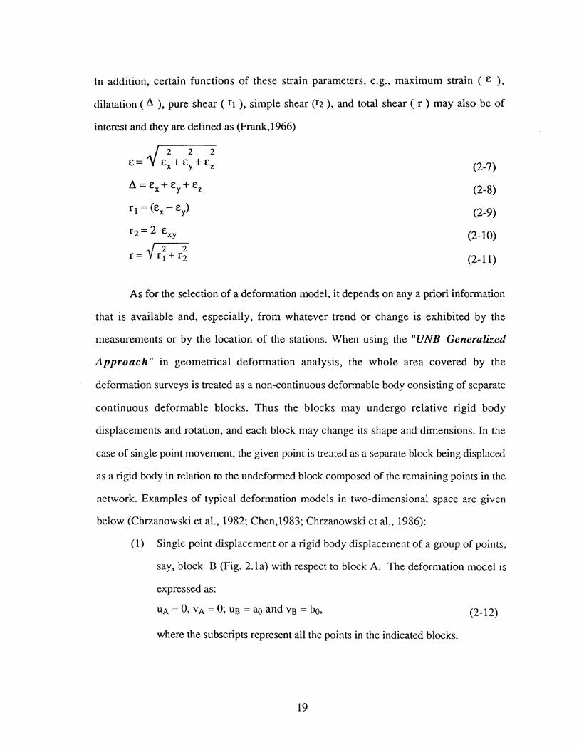
In addition, certain functions of these strain parameters, e.g., maximum strain ( e ),
dilatation ( 11 ), pure shear ( r1 ), simple shear (r2 ), and total shear ( r ) may also be of
interest and they are defined as (Frank, 1966)
_/ 2 2 2 E= 'V Ex+ey+Ez
11 = ex+ ey + e 2
r 1 =(ex- ey)
r2 = 2 exy
r= V ri + r;
(2-7)
(2-8)
(2-9)
(2-10)
(2-11)
As for the selection of a deformation model, it depends on any a priori information
that is available and, especially, from whatever trend or change is exhibited by the
measurements or by the location of the stations. When using the "UNB Generalized
Approach" in geometrical deformation analysis, the whole area covered by the
deformation surveys is treated as a non-continuous deformable body consisting of separate
continuous deformable blocks. Thus the blocks may undergo relative rigid body
displacements and rotation, and each block may change its shape and dimensions. In the
case of single point movement, the given point is treated as a separate block being displaced
as a rigid body in relation to the undeformed block composed of the remaining points in the
network. Examples of typical deformation models in two-dimensional space are given
below (Chrzanowski et al., 1982; Chen,1983; Chrzanowski et al., 1986):
(1) Single point displacement or a rigid body displacement of a group of points,
say, block B (Fig. 2.la) with respect to block A. The deformation model is
expressed as:
llA = 0, VA = 0; Us = <l{) and VB = bo, (2-12)
where the subscripts represent all the points in the indicated blocks.
19

(2) Homogeneous strain in the whole body and differential rotation (Fig. 2.1 b),
the deformation model is
U = Ex X + Exy y - (l) y
V = Exy X + Ey y +(l) X (2-13)
where the physical meaning of the coefficients is defined in Eq.(2-4) to (2-6)
with roz in Eq.(2-6) being replaced by ro.
(3) A deformable body with one discontinuity (Fig. 2.1c), say, between blocks
A and B, and with different linear deformations in each block plus a rigid
body displacement of B with respect to A. Then the deformation model is
written as
U A= ExA X + Exy A Y - (!)A y
VA= ExyAX +£yAY+ (l)A X
and
u B = ao +Exs< x - xo)+ExyB( Y - Yo) - roB (y -yo)
vB = b0 +ExyB( x - x0)+EysC y- y0) + ffis (x -x0)
where xo, Yo are the coordinates of any point in block B
(2-14)
(2-15)
The components ~ui and~ vi of a total relative dislocation at any point i located on
the discontinuity line between blocks A and B can be calculated as
~ui = us(xi,Yi)- uA(xi,yi)
~vi= vs(xi.Yi)- v A(xi·YD
20
(2-16)

y
a) b) c)
~ ~I B 1~ A A,B L _ __ _j
~ A 7~ ---X
Fig. 2.1: Typical deformation models (after Chrzanowski et al., 1983)
Usually, the actual deformation model is a combination of the above simple models
or, if more complicated, it is expressed by non-linear displacement functions which require
the fitting of higher order polynomials or other suitable functions. If time dependent
deformation parameters are sought, then the above deformation models will contain time
variables. For instance, in the model of homogeneous strain, if a linear time dependence is
assumed, the model becomes:
u(x , y , t) = Ex x t + Exy y t - W y t
v(x , y , t) = Exy x t + f.y y t + W x t
2.2 Geodetic and Non-Geodetic Methods for Deformation Monitoring
(2-17)
Acquisition of deformation parameters is one of the main goals of deformation
monitoring. Different methodologies and techniques have been used for this purpose. As
compared with other types of surveys, deformation measurements have the following
characteristics ( Chen, 1983):
(i) Higher accuracy requirement;
21

For example, in engineering projects, an accuracy of± 1 mm or higher might
be a typical requirement
(ii) Repeatability of obseiVations;
The periods of resurveys range from seconds to years, depending on the rate
of deformation
(iii) Integration of different types of obseiVations;
Here not only geodetic methods should be considered but also non
geodetic instrumentation, e.g., pendula, tiltmeters, strainmeters, mechanical
and laser alignment, hydrostatic levels and others in order to get more
complete information
(iv) Network may be incomplete, scattered in space and time;
(v) Sophisticated analysis of the acquired data in order to avoid the
misinterpretation of measuring errors as deformation and local phenomena as
a global status.
Geodetic methods, which include terrestrial geodetic methods, photogrammetric
methods, and space techniques, are used to monitor the magnitude and rate of horizontal
and vertical deformations of structures, the ground surface, and accessible parts of
subsurface instruments in a wide variety of construction situations. Frequently, these
methods are entirely adequate for deformation monitoring. In non-geodetic methods, we
have geotechnical and specialized monitoring devices. They are required only if greater
accuracy is sought or if measuring points are inaccessible to geodetic methods. However,
in general, whenever non-geodetic instruments are used to monitor deformation, geodetic
methods are also used to relate measurements to a reference datum.
Up to now, there are hundreds of available models of various geodetic and non
geodetic instruments for deformation measurements. The decision on which instruments
should be used and where they should be located leads to the need for a proper design and
22

optimization of a proposed measuring scheme which should be based on the best possible
combination of all the available measuring instrumentation. In discussing geotechnical
instrumentation for performance monitoring, Peck (in Dunnicliff, 1988) states that
" ... every instrument on a project should be selected and placed to assist answering a specific question, the wrong instruments in the wrong places provide information that may at best be confusing and at worst divert attention from telltale signs of trouble. Too much instrumentation is wasteful and may disillusion those who pay the bills, while too little, arising from a desire to save money, can be more than false economy: it can even be dangerous ... "
Therefore, the design of a monitoring scheme should satisfy not only the best geometrical
strength of the network of the observation stations, as is the case in geodetic positioning
surveys, but should primarily satisfy the needs of the subsequent physical interpretation of
the monitoring results, i.e., should give optimal results when solving for the deformation
parameters of the selected deformation model (Chrzanowski et al, 1986) and that is the
main topic of this research.
The Geodetic Methods
According to Chrzanowski (1981), in deformation measurements by geodetic
methods, whether they are performed for monitoring engineering structures or ground
subsidence in mining areas or tectonic movements, the monitoring networks can be divided
into relative networks and reference networks (see Fig. 2.2 and Fig. 2.3).
In relative networks, all the survey points are assumed to be located on the
deformable body, the purpose in this case is to identify the deformation model, i.e., to
distinguish, on the basis of repeated geodetic observations, between the deformations
caused by the extension and shearing strains, by the relative rigid body displacements, and
by the single point displacements. However, in reference networks, some of the points are,
or are assumed to be, outside the deformable body (object) thus serving as reference points
for the determination of absolute displacements of the object points.
23

Fig. 2.2: A Reference Monitoring Network
Fig. 2.3: A Relative Monitoring Network
24

Table 2.1: The geodetic methods for deformation monitoring
Methods
i) Elevations by optical levelling
ii) Distance measurements with tapes or wires
iii) Offsets from a baseline using theodolite and scale
iv) Traversing
v) Triangulation
vi) Electronic distance Measurement (EDM)
vii) Trigonometric levelling
viii) Photogrammetric methods
(ix) Space techniques
VLBI SLR GPS
Achievable accuracy (cr)
0.1 mm over a few tens of metres to about 1 mm over long distance
0.1 mm over a few metres to about 2 ppm over a few hundred metres
0.3 - 2 mm
1/30,000 - 1/150,000
1/30,000 - 1/1,000,000
0.2 mm or 0.1 ppm to 5 ppm
2 mm Ykm
l/5000 - 1/100,000
0.01 ppm 0.01 ppm O.lppm - 2 ppm
25

Table 2.2: The Non-Geodetic Methods for Deformation Monitoring
Types of deformation Methods and sample Typical accuracy instruments
a) Wire and Tape extensometers
* ISETH Distometer 0.05 mm * CERN Distinvar 0.05 mm *Rock Spy 0.02 - 0.2 mm
b) Rod and Tube Extensions and strains extensometers
* Single-point 0.01 - 0.02 mm ex tensometers * Multi-point 0.01 - 0.02 mm extenso meters * Torpedo type
ex tensometers 0.1 mm
c) Michelson type laser interferometers
* Laser strain meters 0.0004 ppm
a) Precision tiltmeters * High precision
mercury tiltmeter 0.0002" *Electrolcvel 0.25" * Talyvel 0.5''
Tilts and inclinations b) Hydrostatic levelling *Elwaag001 0.03 mm/40 m * Nivomatic
telenivelling system 0.1 mm/ 24 m
c) Suspended and Inverted Pendulum 0.1 mm
a) Mechanical Methods * Steel wire alignment 0.1 mm * nylon line alignment 0.035 mm - 0.070 mm
Alignment b) Direct Optical alignment 1- 10 ppm c) Alignment with laser
diffraction gratings 0.1 - 1 ppm
26

A list of the most commonly used geodetic methods for deformation monitoring and
their associated approximate accuracies is given by Table 2.1. Over the last 20 years the
availability of increasingly reliable and accurate EDM equipment has radically changed
conventional surveying practices. EDM devices require fewer personnel than conventional
optical instruments, are faster to use, and are more accurate. Therefore, horizontal
triangulation monitoring networks have been gradually replaced by trilateration or
triangulateration networks. Depending on the models, an EDM instrument can have a range
of a few meters to several tens of kilometres. Recent progress in distance measurements
includes the develop~ent of the multiple wavelength EDM to reduce the effect of
tropospheric refraction internally, e.g., Terrarneter (Hugget, 1982) and the EDM with high
modulation frequencies, e.g. Kern ME 5000. The former can achieve an accuracy in the
order of 0.1 ppm over distance of several kilometres while the latter can give 0.3 mm
standard deviation over a few hundred meters.
Trigonometric levelling is much more economical than conventional geodetic
levelling when third-order accuracy is adequate and measuring points are physically
inaccessible. According to Chrzanowski (1983), even the first order and second order
accuracy can be achieved by a modified trigonometric levelling i.e. the leap-frog OI:"
reciprocal trigonometric levelling. This method is especially advantageous in mountainous
areas.
Both terrestrial and aerial photogrammetry have been extensively used in the
determination of deformations of large structures (e.g. Faig, 1978), and ground
subsidence(Faig and Armenakis, 1982). In terrestrial photogrammetry, an example is to use
phototheodolites to take successive photographs from a fixed station along a fixed baseline.
Movements are identified in a stereocomparator by stereoscopic advance or recession of
pairs of photographic plates in relation to stable background elements. The procedure
defines the components of movements taking place in the plane of the photograph. The
27

photogrammetric methoo has the advantage that hundreds of potential movements are
recorded on a single stereo photographic pair, allowing an appraisal of the overall
displacement pattern in a minimum time.
Ge<Xietic space techniques, e.g. VLBI(Very Long Base Line Interferometry), SLR
(Satellite Laser Ranging), and GPS (Global Positioning System) can provide deformation
data of global extent, such as polar motion, variation of the earth's rotation, and relative
motion between tectonic plates.
The Non-Geodetic Methods
The ge<Xietic methoos, through interconnections among the monitoring stations, can
provide very useful information on the global deformation status of the monitored object
and, in most cases, can also provide information on its rigid booy translations and rotations
with respect to reference points located outside the deformation area. However, as
mentioned above, geodetic methods are limited only to open areas, they require
intervisibility between the survey stations, or between the monitoring stations and the
satellites, or between the object points and the cameras. The deformations inside the
deformable body e.g. in foundations or foundation rocks of large engineering structures
and relative movements of different layers of soil or rock formations in slope stability
studies, etc, can only be approached by non-geodetic methods.
Non-geodetic methods include geotechnical instrumentation and other specialized
monitoring devices. For instance, borehole inclinometers, extensometers, are examples of
geotechnical instruments, while inverted pendula, hydrostatic levels, laser interferometers,
and diffraction aligning equipment, are made for some specialized monitoring purposes.
Geotechnical instrumentation does not require intervisibility between the stations and can be
easily adapted for continuous and telemetric data acquisition with an instantaneous display
of the deformations which is very advantageous in comparison with slow, labour intensive,
geodetic surveys. Non-geodetic methods are usually used to measure three types of
28

deformations, i.e. extensions and strains; tilts and inclinations; and alignment. Typical
examples of Non-Geodetic Instruments with their associated accuracies are listed in Table
2.2 (Chrzanowski, 1986).
One has to remember that the non-geodetic methods, despite their indisputable
advantages, also have weak points: a) the measurements are very localized and they may be
affected by local disturbances which do not represent the actual deformations; b) since the
local observables are not geometrically connected with observables at other monitoring
stations, and global trend analysis of the deformations is much more difficult than in the
case of geodetic surveys unless the observing stations are very densely spaced
(Chrzanowski, 1986).
2.3 Estimation of Deformation Models and the Design Problem
2.3.1 The functional relationship between the deformation models and the observed
quantities.
Any observation, geodetic or non-geodetic measurement made in deformation
surveys, will contribute to the determination of deformation parameters and should be fully
utilized in the analysis(Chrzanowski et al., 1986; Teskey, 1987). The functional
relationships between different observable types and the selected deformation model are
given below using a local geodetic coordinate system (Chen, 1983)
(1) Observation of coordinates of point i, for instance, the coordinates derived
from photogrammetric measurements or obtained using space techniques:
( Xj(t) l (Xi(to)l (Uj l Yi(t) = Yi(to) + Vi Zj(t) Zj(tQ) Wj
(2-18)
29

(2) Observation of coordinate differences between points i and j, e.g., height
difference (levelling) observation, pendulum (displacement) measurement,
and alignment survey:
(Xj(t)- Xi(t) ) ( Xj(to)- Xi(to)) ( Uj- Uj) Yj(t)- Yi(t) = Yj(to)- Yi(to) + Vj- Vi
Zj(t)- Zi(t) Zj(l{))- Zi(to) Wj- Wj
(2-19)
If the components of the displacement obtained from a pendulum observation
do not coincide with the coordinate axes, a transformation to the common
coordinate system has to be performed. Similarly, a coordinate transformation
may be required in alignment surveys which provide a transverse
displacement of a point with respect to a straight line defined by two base
points.
(3) Observation of azimuth from point i to point j
(2-20)
where ~ij and Sij are the vertical angle and spatial distance from point i to
point j, respectively. The observation of a horizontal angle is expressed as the
difference of two azimuths.
( 4) Observation of the distance between points i and j:
(2-21)
(5) Observation of strain along the azimuth a and vertical angle J3 at point i:
30
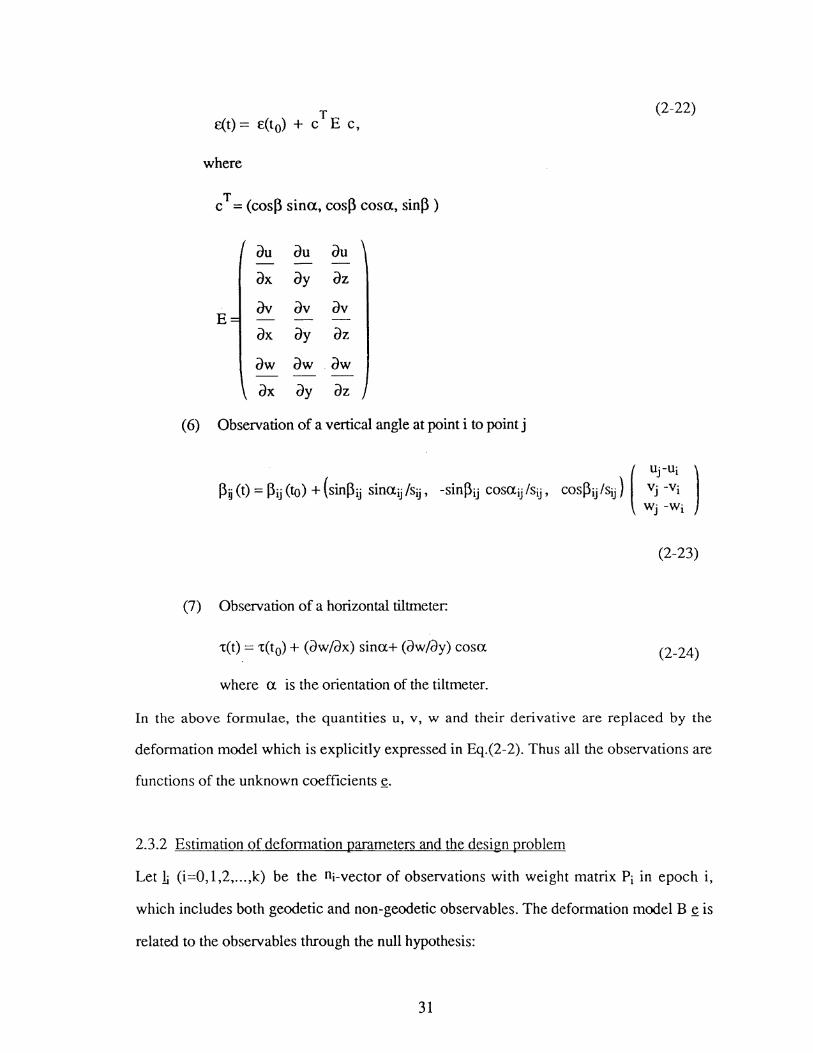
T E(t) = E(t0) + C E C,
(2-22)
where
c T = (cosJ3 sin a, cosJ3 cosa, sinJ3 )
au au au
ax ay az
E av av av
ax ()y dZ
aw dW . dW
dX ()y az
(6) Observation of a vertical angle at point i to point j
(2-23)
(7) Observation of a horizontal tiltmeter:
-r(t) = -r(t0) + (aw/ax) sina+ (iJw/ay) cosa (2-24)
where a is the orientation of the tiltmeter.
In the above formulae, the quantities u, v, w and their derivative are replaced by the
deformation model which is explicitly expressed in Eq.(2-2). Thus all the observations are
functions of the unknown coefficients ~-
2.3.2 Estimation of deformation parameters and the design problem
Let 1 (i=O, 1,2, ... ,k) be the ni-vector of observations with weight matrix Pi in epoch i,
which includes both geodetic and non-geodetic observables. The deformation model B ~ is
related to the observables through the null hypothesis:
31

Ho: E(hl=E(_lo)+~ ~ ~ (2-25)
where ~ is the configuration matrix which relates the observables to deformation model;
Bi is the coefficient matrix of deformation model, it is a function of position and
time; and
~ is the vector of deformation parameters.
The parameters~ may be estimated from the following mathematical model
lo h
.Yo
+ Yl
I I (!) (2-26)
with~ being a vector of nuisance parameters and the weight matrix (assuming there is no
correlation between epochs)
Po 0 0 0 0 p1 0 0
P= (2-27) 0 0 pk-1 0 0 0 0 pk
Applying the least squares criterion to the above model and eliminating 5_ allow the vector
of deformation parameters ~ and its accuracy to be calculated from
1 1
k TT k TT k 1k *("B·A·P·l·-"B·A·P·("P·)- "P·l·) £... I I I I £... 1 1 I £... 1 £... I -1
(2-28)
1 1 0 0
k k k k
I T T I T T I -li -1 n-=( B·A·P·.A·B·- B-AP·( P·) P-AB·) '<!;< 1 1 i:' '1 1 1 1 1 1 1 1 1 (2-29)
1 1 0 1
32

In the design phase it is justified to assume that the observation schemes are the
same for all the epochs (i.e. Ai=A, Pi = P, for all i). And the expression for the estimation
and accuracy of the estimated deformation parameters can be obtained by considering only
two epoches. Therefore,
~=(BTATPABtlBTATP(h- h)
~=2(BTATPAByt
(2-30)
(2-31)
When B=l (identity matrix), then the deformation monitoring reduces to determine the
displacements of object points. In this case, the cofactor matrix of the displacements can be
expressed by
Qg=2(ATPAt (2-32)
The design problem involves how to find the best configuration matrix (A) and the weight
matrix (P) in order to attain the required accuracies of the deformation parameters or
displacements in the mosteconomical way.
33


CHAPTER 3
QUALITY CONTROL MEASURES AND OPTIMALITY
CRITERIA FOR DEFORMATION MONITORING SCHEMES
Generally, the quality of a monitoring scheme may be characterized by precision,
reliability, sensitivity and economy. Precision, as expressed by the a posteriori covariance
matrix of the coordinates, displacements, or deformation parameters, etc, is the measure of
the scheme's characteristics in propagating random errors; reliability describes the ability of
the redundant observations to check observation errors; sensitivity describes the scheme's
ability to detect postulated displacements or deformation parameters of certain magnitude;
and finally, economy is expressed in terms of the observation program. Thus the
optimization of a monitoring scheme may be said to design a precise-, reliable- and
sensitive enough scheme which can also be realized in an economical way. But how
precise, reliable, sensitive and cheap should the scheme be? A quantification of the
demands is obviously indispensable. This chapter will discuss various measures and
criteria for these different indicators of the quality of a monitoring scheme, and this serves
as the foundation for the optimization.
34

3.1 Measures and Criteria for Precision
3.1.1 Scalar precision functions
A great deal of work has been carried out in the field of user precision requirements
for geodetic networks. In the case of integrated monitoring schemes with geodetic and non
geodetic instruments, since the displacements or deformation parameters to be monitored
can be derived from changes in point coordinates, thus a good knowledge of the ways to
quantify the precision of geodetic networks is fundamental for us to properly establish
precision measures and criteria for monitoring schemes.
The precision in geodetic networks is expressed in terms of the variance-covariance
matrix of the point coordinates Cx or of estimable quantities derived from coordinates Cr.
The purpose for which a network must serve is decisive for the determination of the
precision required. In the case of multi-purpose networks (such as national control
networks whose purpose may not be specified), it is difficult to establish a link between
social values (related with the purpose) and geodetic numerical indicators of quality, while
it is much easier for networks with limited and specific purposes. For instance, when
defining a geodetic network for setting out an engineering structure, for controlling the
breakthrough of tunnelling or for providing photogrammetric control, there may be quite
special requirements e.g. the accuracy of certain functions pertaining to specific points or
group of points. Thus to quantify the required precision is often quite straightforward. In
the case of the general purpose networks, however, the precision requirements cannot be
specified so easily. In such cases it is necessary to have some concepts of " ideal "
networks. These ideal precision criteria can either be based on theoretic results, such as
those of Grafarend(1972), on homogeneous and isotropic networks (Taylor-Karman
Structure), or they can be derived from empirical studies with real networks.
One measure of precision takes the form of a scalar function of the elements of the
covariance matrix of the coordinate variates. The purpose is to fill the need for an overall
35

representation of the precision of a network. A scalar function may be one of the
following(Grafarend, 197 4)
i) N-Optjmality
f= II ~II --> min
with II · II denoting the norm of a matrix;
ii) A-Optimality
f =Trace(<;_) =A. 1 + A. 2 + ··· + "-r -->min
with A. 1 , A. 2 , ... , "-r the non-zero eigenvalues of the matrix C.!;
iii) E-Optimality
f= "-max -->min
with A. max the maximum eigenvalue of matrix C.!;
iv) S-Optimality
f= (A. - A. . ) -->min max mm
with C"-max- "-min) the spectral width of matrix Cli;
v) D-Optimality
f = Det( Cr)= A. 1 * A. 2 * ... * "-r -->min
(3-1)
(3-2)
(3-3)
(3-4)
(3-5)
where Cr = diag(A. 1 , ... , ').._r) with A. 1 , ... , "-r the non-zero eigenvalues of the
covariance matrix eli·
If we demand some certain function f of coordinates x..
f=cT X - _, (3-6)
to have the highest precision, then a criterion may be written as
cr= ~T Cx ~ -->min (3-7)
where ~ is a vector of constants.
There may be other scalar precision measures, depending on the purpose of the designed
networks.
36

The advantage of trace, determinant, and eigenvalues of a covariance matrix is that
they all are datum-independent quantities. However, the disadvantage is that an overall
precision criterion does not control individual values. In addition, on account of correlation
between the coordinate variates of different points, coordinate variances alone are not
capable of representing variances of operational variates such as angles or distances. For
instance, Mittermayer (1972) shows that the small coordinate variances produced by a
minimum trace matrix can be deceptive. In his example of a trilateration network, the
variances of adjusted distances will be the same whether they are computed from the
minimum trace matrix or from a covariance matrix based on any other correct reference
system. Sc~ar measures are rather coarse characteristics of the covariance matrix. They can
be used as criteria for the comparison of different designs and for minimization, but they
are difficult to be used as an absolute criterion, whose numerical value is, for instance,
required not to surpass a certain pre-assigned value related to the purpose of the network.
Therefore, the application of scalar precision measures in practice is limited.
3.1.2 Criterion matrices
A much more detailed control of precision is provided by a criterion matrix. A
criterion matrix is an artificial variance-covariance matrix possessing an ideal structure,
where "ideal" means that it represents the optimal accuracy situation in the planned
network. If, instead of a scalar risk function, a criterion matrix is introduced in an optimal
design procedure, the solution to the optimization problem must approximate it as closely
as possible.
The structure of the criterion matrix for general purpose networks, such as the
control networks for regional or national mapping, has been extensively studied by
Grafarend (1972) and Baarda (1973). The results are in the form of the general Tayler
Karman structured criterion matrix or its chaotic structure.
37
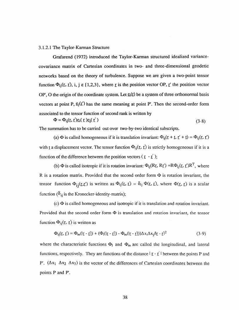
3.1.2.1 The Taylor-Karman Structure
Grafarend (1972) introduced the Taylor-Karman structured idealized variance-
covariance matrix of Cartesian coordinates in two- and three-dimensional geodetic
networks based on the theory of turbulence. Suppose we are given a two-point tensor
function <l>ij(!:, r), i, j E ( 1,2,3}, where r is the position vector OP, r' the position vector
OP', 0 the origin of the coordinate system. Let~(!) be a system of three orthonormal basis
vectors at point P, ~j(r') has the same meaning at point P'. Then the second-order form
associated to the tensor function of second rank is written by
<l> = <l>ij(£, r)~C r )~j( i ) (3-8)
The summation has to be carried out over two-by-two identical subscripts.
(a) <l> is called homogeneous if it is translation invariant: <l>ij(I + 1, r' +!) = <l>ij(I. r')
with! a displacement vector. The tensor function <l>ij(I, r) is strictly homogeneous if it is a
function of the difference between the position vectors ( r -i ); (b) <l> is called isotropic if it is rotation invariant: <l>ij(Rr, Rr') =R <l>ij(r, r')R T, where
R is a rotation matrix. Provided that the second order form <I> is rotation invariant, the
tensor function <l>ijCr..r.') is written as <l>ij(r., r) = Oij <l>(r., r.), where <l>(r, r) is a scalar
function (Oij is the Kronecker-identity-matrix);
(c) <1> is called homogeneous and isotropic if it is translation and rotation invariant.
Provided that the second order form <1> is translation and rotation invariant, the tensor
function <I>ij(L r.) is written as
(3-9)
where the characteristic functions <l>j and <I>m are called the longitudinal, and lateral
functions, respectively. They are functions of the distance I I- r' I between the points P and
P'. (~xl ~x2 ~x3) is the vector of the differences of Cartesian coordinates between the
points P and P'.
38

Eq.(3-9) has been named after Taylor (1935) and Karman (1937) and was
introduced to geodesy by Grafarend(1972). By applying the two- point tensor function on
geodetic networks, for the special case of homogeneity and isotropy, an expression for the
submatrix of cross-covariance between points Pi and Pj on the plane within the TK-
structured criterion matrix equals to (Grafarend, 1972):
4d2 4d where «<> (s) =- -2 k0(s/d) - - k 1(s/d)
m 2 S s
4d2 4d 2s <I> 1(s) =--2 +2k0(s/d)+ -s-k 1(s/d)~k 1(s/d)
s
s =I ri- rj I =1 (xi-xj)2 + (yi-Yj)2
(3-11)
(3-12)
(3-13)
in which ko and kt are the modified Bessel functions of the second degree and of zeroth
and first order, d is the characteristic length. The magnitude of the characteristic distance d
of a network still remains a problem. For example, according to Schmitt(l980), d should
be chosen smaller than the minimum distance between any arbitrary two points of the
network, while Wimmer(l982) recommends the maximum distance (or diameter) of the
network as an upper bound for 10 d.
3.1.2.2 The Chaotic Structure
Eq.(3-10) leads to an error situation characterized by identical error circles at the
netpoints. However, Baarda(l973) and Alberda (1974) proposed to use a special case of
this structure called the "chaotic structure". In that case, the relative error ellipses are
39

also circles with a radius which depends on the distance between the points to which they
refer. They adopted the following relation
<I>m(s) = <l>t(s) = d2 - r2s, r2>0 (3-14)
for a suitable constant r2. The submatrix of cross-covariance between points Pi and Pj on
the plane is
0 d2-dij 0
d2 0 d2- d7. lJ
(3-15)
symmetric d2 0
d2
where d2 =constant; and
d~ = d~ =f(li) is a positive monotonic non-decreasing function of the side length
lij· The d2 and d~ should be chosen so that C is positive definite. However, the variance
covariances of all kinds of coordinate differences do not have anything to do with d2. For
example, fori, j :;t:l:
(3-16)
(3-17)
From Eq. (3-16) and (3-17), we can see that by subtracting x1 and Yl from all other Xi and
Yi we obtain new coordinate variates whose covariance matrix does not contain d2 any
more. So it plays no role in the formulation of the criterion matrix for precision, only the 2
function dij is important. It is called the "Choice function" because one can choose this
function to set a criterion. This function should be defined so that the transformed criterion
matrix referred to aS-base Cs is positive definite. Baarda (1973) proposed that
40

(3-18)
This function has been used in Netherlands for network reconnaissance. Alternative
choices are ( Karadaidis, 1984; Meissl, 1976)
or
2 2 lij 2 dij = c 1 c2 In { 1 ~} + c0
c2 (3-19)
(3-20)
Other choices are possible too. The actual choice of the function depends on the type of the
network. Once a choice has been made, the parameters Co, Ct and c2 can be used to set the
actual criterion for precision. This may depend on the class of network e.g.: densification
level, terrain type, etc.
3.1.2.3 Modification of the Present Covariance Matrix
For special purpose networks such as met in civil engineering and deformation
measurements, the elements of the criterion matrix can be computed from user
requirements, such as the shape of error ellipses or the accuracy of derived quantities. In
this respect, an example was given by Koch (1982). He suggested to construct a criterion
matrix by modifying the present covariance matrix of coordinates of geodetic netpoints in
the following way:
" " Let (xi, y j) and (x j• y j) be the estimates of the projected coordinates of two points
of a two-dimensional network and let their variance-covariances be given by
41

By the law of error propagation the covariance matrix of the coordinates differences
(~i• y) and (~j• Y} of the two points follow
symmetric
O'xiYi- O'xi)';- O'x;yi + O'x;y; l <fyi +<fyi -20'y;yi
A confidence ellipse of circular shape follows for the first point from the equality
1 1 2 2
(ax;-O'Y~ + (2axy~ =0
which is satisfied by
1 2
ax.= ay_and ax.,.=O l 1 Ill
and for the second point by
If, in addition
a = a and a =- a X/<-i YYi Yl<-i xy,
(3-22)
(3-23)
(3-24)
(3-25)
then a relative confidence ellipse of circular shape is obtained for the coordinate differences
of the two points.
Let C.!. be the covariance matrix of the coordinates of the network to be optimized,
the elements of the covariance matrix for the points to be optimized are then changed
according to Eq.(3-23)- (3-i5) so that smaller confidence ellipses with circular shapes for
the coordinates and the coordinate differences of these points are obtained. This changed
covariance matrix is then used as the criterion matrix for the optimization.
In deformation monitoring, the parameters of interest are usually displacements@
or deformation parameters ~) derived from observations in the monitoring scheme as
expressed by
42

..... with the corresponding covariance matrices for d • a obtained from
~ =C!1 + C!2 =2Cx (in the design phase)
(in the design phase)
(3-26)
(3-27)
(3-28)
(3-29)
where x1 , & represents the estimates of the vector of coordinates in two different
measurement epoches; a. and ~ are the vector of displacements and deformation parameters
respectively; and B is the coefficient matrix of the deformation model.
At first, the scalar precision measures of geodetic networks may be directly adopted
for monitoring schemes by substituting Cg_ and Cs:. for~ in Eq. (3-1) - Eq.(3-7), i.e.,
i) f= II Cg_ or C.s;..ll --> min;
ii) f = Trace( Cg_ or Cs;. ) --> min;
iii) f= A. max -->min
with A. max being the maximum eigenvalue of matrix Cg_ or C~;
iv) f= (A. max- A. min) -->min
with (A max- A. min) being the spectral width of matrix Cg_ or C!1;
v) f = Det( C-)
- A. A. A. -->min - 1* 2*•••* r
(3-30)
(3-31)
(3-32)
(3-33)
(3-34)
where Cr = diag(A. 1, ... , A.r) with A. 1, ••. , A.r the non-zero eigenvalues of the
covariance matrix Cd or Ce · - _,
vi) if we demand that some certain function f of d or ~ '
f= c T d or c T e - - - -' (3-35)
43

has the highest precision, then a criterion may be in the form:
Cf = ~T Cd ~ or ~T Ce ~ -->min (3-36)
where £ is a vector of constants
There may be many more other scalar precision measures, depending on one's purpose.
The criterion matrix for displacements and deformation parameters can be
approached in different ways. At ftrst, if the criterion matrix for point coordinates q is
established, then from Eq.(3-28) and Eq.(3-29) we have the criterion matrix for
displacements Cd and deformation parameters G as
Cd=2 ex Q=2 (BT(qyt BYl
(3-37)
(3-38)
where q may take the form of homogeneous and isotropic precision or may be constructed
by modifying the present covariance matrix of coordinates. The problem for this approach
is that the precision of deformation parameters is not controlled, since good precision of
coordinates may ensure good precision of displacements but may not ensure good precision
of deformation parameters. Thus the criterion matrix for deformation parameters may also
be obtained by modifying the present covariance matrix q of deformation parameters
according to the required precision for each individual parameter e;. (i=1, ... , u). Once the
criterion matrix for deformation parameters is properly defined, and since
(3-39)
then a solution for the criterion matrix of displacements and coordinates can be (Schaffrin et
al., 1977; Schaffrin and Grafarend, 1982):
Cg = ((BT)+ ~~ s+ )·
= (B (BTBy1 ~~ ( BT BY1 BT)- (if BTB is non-singular)
and from Eq. 3-37), we have
44
(3-40)

(3-41)
Obviously this corresponds to a minimum norm solution of the system of equations (3-39).
Another approach to construct the criterion matrix for displacements was studied by
Sprinsky(l978),Wimmer(1981), and Crosilla(l982;1983). They proposed to construct a
criterion matrix for displacements to be monitored by contracting the eigenvalue spectrum
of the covariance matrix of the adjusted network coordinates and/or by rotating the m-
dimensional error ellipsoid to redistribute the allocated variance. A review of this technique
is given below:
Referring to Eq.(3-26) and Eq.(3-28), an estimated (m-dimensional) displacement ,..
vector~ may be defined as the difference between two estimated coordinate vectors and
relating to different measurement epoches:
with covariance matrix
In the hypothesis of a least-squares minimum norm solution for a free net
rank(Cd} = h< m (3-42)
The quadratic form
r.
with g the expectation of~ (3-43) r.
corresponds to the equation of an h-dimensional error ellipsoid, centered in~ in which the
length of the semi-axes and their directions are given by the square root of the eigenvalues
greater than zero, and the corresponding eigenvectors of c;; respectively:
(3-44)
45

where A1 = diag ( A. 1, A.2 , ... , A.h)
with A. 1 ~ A. 2 ~ ... ~ A.h > 0
(3-45)
V1 and V2 are the submatrices of the eigenvectors relating to the non-zero
eigenvalues and zero eigenvalues respectively.
At the first stage, the contraction of the eigenvalue spectrum may be accomplished
using a "contraction parameter t", with 0 ~ t ~ 1, arbitrary but fixed in two different
formulations
(3-46)
A.i =min (A.i, A. 1) fori= 2, ... , h ( Sprinsky,1978; Wimmer, 1982)
(3-47)
At the second stage, if a deformation is defined by means of a prediction method,
the worst directions to detect point movements are those which correspond to the direction
of the greater semi -axes of the error ellipsoid, that is, the eigenvectors relating to the greater
eigenvalues of c;; . According to the conceived deformation model, it might be useful to
proceed with some rotations of the component pairs of the essential eigenvector in such a
way that they would be oriented as close as possible along a direction orthogonal to that of
the movement predicted by the deformation model. For a sound statistical study of the ~
displacement vector Q_, based on the analysis of the principal components(Niemeier, 1982) it
is necessary to investigate a total variance percentage equal to 40- 60% of tr(c:J ).
Whenever 'A 1 alone represents such a value it is sufficient to rotate only the component
pairs of the first eigenvector. Otherwise, account must be taken of all the eigenvectors
relating to the greatest eigenvalues for which L 'Ai is equal to 40- 60% of tr(Cd ).
One rotation technique involves the rotation equal to an angle <i'x,y of all the pairs of
eigenvector components relating to the coordinates xi, Yi of q netpoints (1 $ q$ m/2):
46

(3-48)
This follows from the fact that in order to ensure the orthogonality of all the h vectors Yt of
V it is necessary to perform the same rotation for all the pairs of elements of the h
eigenvectors relating to the coordinates Xi • Yi of the netpoints.
Another rotation technique is the so-called procrustean transformation of the V 1
112 eigenvector matrix or of the factorial matrix A V~. With the procrustean transformation
each pair of h eigenvector components can be rotated independently. This is of particular
importance in case in which the first eigenvalue A1 does not represent 40 - 60% of the total
variance and it is, therefore, necessary to take more than one eigenvector into consideration
in order to satisfy, from the statistical point of view, the condition of orthogonality between
the pairs of essential eigenvector components and the predicted direction of the movement.
From the independent rotations of each couple of eigenvector components, the resulting
matrix- that is the target matrix Yo, is no longer constituted by orthogonal eigenvectors.
The procrustean transformation (Schonemann, 1966) is to find an orthogonal matrix T
which satisfies the approximation
(3-49)
from the least squares point of view. ......
Finally, the criterion matrix for the displacement vector ~ resulting from the
procrustean transformation technique and from the contraction of the eigenvalue spectrum
can be written as
(3-50)
where A 1 is the matrix of contracted eigenvalues
47

T = X yT with X, Y from the results of the singular value decomposition of matrix
T V1 Yo 1.e.
(3-51)
3.1.3 The datum problem for criterion matrix
The Taylor-Karman structured criterion matrix Eq.(3-10) and Eq.(3-15) refer to a
point field where all coordinates are stochastic. In principle, the criterion matrix should be
created independently of any linear model connecting the sought parameters to certain
observations. However that is not possible in real point fields where a network datum for
coordinates should be defined. In order to make the criterion matrix comparable with a
"real" covariance matrix which has a defined datum, the criterion matrix should be
transformed with the same datum parameters. This transformation may be accomplished
by executing a proper S-transformation (Baarda, 1973; Schaffrin, 1985)
S =I- H (DT H )-1 DT
CTrans. = s c sT (3-52)
where C and CTrans. are the criterion matrices before and after transformation respectively;
I is the identity matrix; H is a matrix satisfying A H =0 with A the configuration matrix of
the network and D characterizes the datum of the network with datum equation D T K =0
and rank(D)= datum defects of the network.
However, if a criterion matrix for datum-independent deformation parameters such
as relative block movements, strain parameters and their derivative is defined in the
optimization procedure, it can be directly used to fit the inverse of the normal equation
matrix of the deformation parameters.
One should remember that although deformation stricti y means change of shape and
dimension, detection of scale changes, rotations and displacements must also be included.
48

In many cases, the deformation parameters are derived from changes in coordinates of the
object points as a result of survey observations made at two or more epoches. The changes
in coordinates (i.e., displacements) of points are the quantities that geodesists and
surveyors like to work with because they allow for an easy identification of the deformation
model for further geometrical analysis (Chrzanowski et al., 1982). However, the use of
"coordinates of points" introduces problems associated with the way in which those
coordinates are defined. i.e., the coordinates are datum-dependent. Although the estimation
of the deformation parameters using the "UNB Generalized Approach" does not
depend on the choice of datum, careful selection of a datum will provide a picture of the
displacement field, which makes it easier to identify the deformation model in the space
domain or to identify the suspected unstable points of a reference network.
At the design phase, the a priori knowledge of the expected deformation is of much
help for the definition of an appropriate datum. Such information comes from a study of the
relevant physical, geomechanic, and/or structural properties of the object. In the absence of
any a priori reliable data about the likely behaviour of points on and around the object it is
necessary in the first instance to assume that all points are subject to deformation, and some
sophisticated techniques can be used to define an appropriate datum at the stage of post
processing of the data (Chrzanowski et al. 1983; Chen 1983; Chrzanowski et al. 1986).
3.2 Measures and Criteria for Reliability
Deformation analysis involves two types of errors: the errors of observations, and
the errors in deformation models. In order to avoid a misinterpretation of systematic errors
or outliers in the observations as deformation phenomena, screening of the observations for
outliers or systematic errors should be done prior to the estimation of the deformation
parameters. This is why in the "UNB Generalized Approach" for deformation
49
analysis, the adjustment of the geodetic monitoring network for the detection of outliers and
systematic errors, whenever possible, occupies the first position.
The concept of reliability of geodetic networks originates from Baarda(1968).
Generally, it refers to the ability of a network to resist against gross errors in the
observations. In this respect, usually the "internal reliability" and "external
reliability" are distinguished. The internal reliability of a network is its ability to allow the
detection of systematic errors by tests of hypothesis made with a specific confidence level
(1- a) and power (1-p), while the external reliability of a network is related to the effect of
undetected errors on the estimated parameters and on their functions.
The reliability of a network depends on the geometry of the network i.e. the
configuration matrix and on the weight matrix of observations, not on the actual
observations. Thus the problem of reliability should be considered at the design stage to
ensure the detection of gross errors as small as possible and to minimize the effects of the
undetected ones on the estimated parameters.
3.2.1 Gross errors and hypothesis testing
From the least squares parametric adjustment of a geodetic network with nc
observables one obtains the estimates of parameters and residuals as
g = (AT P At1 AT Pl
y =(A(A T P At1 AT P - 1)1
(3-53)
(3-54)
where A, P, and 1 represent the configuration matrix, weight matrix and the observations
vector respectively.
Let us assume that the observational value li (i=1, ... , nc) is erroneous by Vli, and
T introduce the vector, V) = ( 0, 0, ···,VIr 0, ... , 0), containing zeros except for Vli at the
i-th position. Thus the observation vector lis changed by Vi l. If the vector Vi l is full it
50

describes a systematic effect on the obserVations. In this case there are two possible
hypothesis:
null hypothesis: H 0 : E(liHo) =Ax_
alternative hypotheses: Ha : E(liHa) = A K + hi Vli (3-55)
with the vector hi describing the effect of the error source on the observation. If we have a
T blunder Vli in li then hi is a unit vector hi = ( 0 • 0 • · · · • 1 • 0 • · · · • 0). If the error source
leads to a systematic effect, hi is full in general and Vli. will be a single additional
parameter, say Sj.
The effect of errors in the observations as described by the alternative hypothesis on
the different estimates is:
Vig= (AT P A)-1ATPVil
ViY~= (A(AT P At1AT P -I)Vil
Since the expectation ,....
E(v) =0
(3-56)
(3-57)
(3-58)
of ~ is known, in contrast to E(~ ), the effect V &,_ of the error onto the residuals can be
easily seen. By studying the effect of an error onto the residuals, we are able to obtain an
estimate for the size of a gross error which then can be used to estimate its influence onto
the unknown parameters.
By denoting R =(I- A(A T P At1 AT P), Eq.(3-57) reads
VV=- R v l (3-59)
The index is omitted here, as the equation holds for general V 1. The matrix R, in general,
is a full matrix. It contains the full information on the geometry of the design with respect
to the influence of observational errors onto the residuals. The effect Vi ~i of an error Vli
in observation li onto the corresponding residual is determined by the i-th diagonal element
ofR:
51
v.~·=-r· v1. 1 1 1 1 (3-60)
where r is the total redundancy of the system. The diagonal elements of Rare obviously
decisive for our analysis. As they sum up to the total redundancy of the system, we call
them " redundancy numbers", i.e., ri can be seen as the contribution of the observation
lito the total redundancy r of the system. And since ri always is between 0 and 1, only a
possibly small part of an error shows in the residuals. On the other hand if we have an ......
indication that observation li is erroneous then from the residual vi we can obtain an --estimate Vli for the size of the error (assuming Vi = V iYi in the presence of gross errors ):
-- V· Vl·=--1
1 r· 1 --The standard deviation of ~. and Vl· are :
1 1
ov, = -lfi <rt;
av=at.f-lfi 11 I
(3-61)
(3-62)
(3-63)
Statistical tests serve to determine whether or not anything has gone wrong with
some basic postulate. In our context, a statistical test must tell whether the residuals give an
indication that a certain prespecified observation is erroneous or not. The test is based on
the test statistic wi which is a function of the observed values 1. The probability density
function, specifically the expectation and the variance of the test statistic, has to be known
for the case where the null hypothesis Ho is true. Good test statistics use all information,
i.e., are sufficient and lead to the best distinction between the null and alternative
hypothesis. According to Baarda(1968), the best test statistic for blunder detection is
-h:r Pv w·- -1 -
1- a0 vfh[ PQyy Phi
(3-64)
which for uncorrelated observations reduces to the standardized residual
...... - v·
W.- 1 1 -
-lfi <rt; (3-65)
52

The influence of an error Vli in li onto the test statistic w i is
v~. 0~ = Vw· =- 1 =
1 1 r:-0'}. ·•lfj
I
VI--If: 1 1 (3-66)
and leads tO a Shift Of the probability density function of Wj by Oj. Oi is Called the non-
centrality parameter. Assuming that the observational errors are normally distributed under
the null hypothesis, then the probability function of wi , under the null and alternative
hypotheses Ho and Ha , is central and non-central normal distribution respectively:
Wi I Ho )!. n (0,1) (3-67)
(3-68)
From Eq.(3-66) we can conclude that the weaker the geometry (i.e. the smaller ri) the
smaller is the influence of a blunder onto the test statistic w i. thus the more difficult it will_
be to discern between Ho and Ha.
Carrying out of the test is shown in Fig. 3.1. The boundary values - w a/2 and
+ w a/2, divide the w-axis into two regions V and W with the following test procedure:
cj>(wjHo) cj>(wiHa)
-Wall +wall
Fig. 3.1 Density functions of test statistic w i
1) If Wi E W i.e. lwi I ~ Wa/2 then accept Ho
2) If Wi E V i.e. lwi I > Wa/2 then reject Ho
53
(3-69)
(3-70)

(3-80)
can be considered as a measure of the reliability of the estimated coordinates.
2 Substituting a 0 from Eq.(3-77) and using the vector hi, Eq.(3-79) becomes
2 1 A.. 0 =30 r-=--1)
1, 'r· 1
(3-81)
Similarly, the influence of undetectable gross errors Vli on the solution of
deformation parameters can be defmed by:
" T T -1 T T Vi . 0 ~ = 2 (B A P A B ) B A PV o, ~ , (3-82)
- 1 " T -1 " J... o =- (Vo · ~ Q (Vo · ~)
1, 2 ,1 ~ ,1
(3-83)
and
A. 0 =max 0-i. 0) (3-84)
A.o is used as a measure of the reliability of the estimated deformation parameters.
Replacing o5< BT AT p A Btl by one half of the criterion matrix of deformation
parameters, i.e., ~ a5 ~ and approximating ri by an average value of r = rfc (Chen et
al., 1983) with r being the total redundancy and IlG the number of geodetic observations in
the geodetic network, we obtain
- s:2 A.o . = uo nc (A B Qc BTAT p )·· .• r !< 11 (3-85)
3.2.3 The optimality criteria
57

Thus gross error larger than the boundary value can be detected. Otherwise, they are not
detectable.
From Eq.(3-77) we can see that the boundary value V o li depends on the precision
of the observation described by the standard deviation O'I;; the geometry of the design of the
measuring procedure described by the redundancy number ri; and the significance level <lo
and the required minimum power ( 1 - 13 o) comprised in the lower bound <>o for the non-
centrality parameter. The smaller the redundancy number ri of the observation, the larger a
gross error has to be in order to be detectable. The case of ri=l occurs only if the true value
of the observation is known. If ri=O then a test of the observation is not possible: the
boundary value is infinite.
3.2.2.2 External reliability
External reliability relates to the maximum effect of possibly undiscovered
observational gross errors VIi on the estimates of unknown parameters (e.g. coordinates,
deformation parameters). The influence of VIi on coordinates i.e. V o, i i. is given by
(3-78)
Since V o, i i. is datum dependent, Baarda (1976) proposed a new standardized variate
1 ,..... T -1 ,..... /.... o=-(Vo -~ Qy (Vo -x)
I , 2 , I .a , I (3-79)
which is invariant with respect to the coordinates defined. However, one is interested
mainly in the maximum value of this variate which is related to the minimum deviation from
the null hypothesis that can be detected with a certain probability Po. So the following
variate (Baarda, 1976)
56

It is possible that this test leads to a wrong decision, which is called an error of Type I or
Type II. The probabilities for these errors are given by
Type I error: a =p{ Wi E VIHo} = 2 ( 1-<l>(wa/2)
Type II error: (3 =p{ Wi E W IHa } = <l>(wa/2- Oi)- <1>(- Wa/2- Oi)
where <l>(w) is the normal distribution function.
(3-71)
(3-72)
Physically, a is the probability that the observation is error free but one may
conclude from I Wi I> ~N(O,l). 1-a./l that it contains an error, and is called the significance
level. (3 is the probability that the observation is erroneous but one may conclude from
I Wi I ~ ~N(O,t),l-<tfl that the observation is correct 1- (3 is called the power of the test. Since
the actual value Vli of a gross error and thereby the non-centrality parameter oi is not
known, the probability (3 can not be computed in practice. Baarda(1968) proposed to invert
the relation between the power of the test and the non-centrality parameter and use
o =o ((3, a) (3-73)
For a preset power of the test, Eq.(3-73) gives the distance between H 0 and Ha. i.e. the
size of the error which can be detected with that power. If we now require that an
alternative, i.e. an error has to be detected with a probability of 1- (3 which is larger than a
prescribed bound 1-(30 then the distance o between Ho and Ha has to be larger than the
bound Oo i.e.
1 - (3 > 1 - 13o --> o >oo, oo = o(J3o, ao) (3-74)
As for the calculation of Oo, from Eq.(3-72), the second term is usually very small if
Oi > 0. If Oi is larger than Waf2 then the term can be neglected and we obtain
(3-75)
When ao, J3o are fixed, the noncentrality parameter can be computed from
-1 Oo = wao 12 - <1> ( J3o ) (3-76)
54
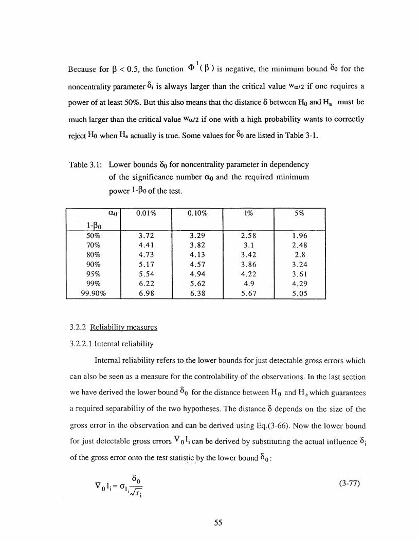
Because for p < 0.5, the function <l>-1 ( P ) is negative, the minimum bound oo for the
noncentrality parameter Oi is always larger than the critical value Waf2 if one requires a
power of at least 50%. But this also means that the distance o between ~ and Ha must be
much larger than the critical value Wa/2 if one with a high probability wants to correctly
reject Ho when Ha actually is true. Some values for Oo are listed in Table 3-1.
Table 3.1: Lower bounds 8o for noncentrality parameter in dependency
of the significance number ao and the required minimum
power 1-Po of the test.
ao 0.01% 0.10% 1% 5%
1-Po 50% 3.72 3.29 2.58 1.96 70% 4.41 3.82 3.1 2.48 80% 4.73 4.13 3.42 2.8 90% 5.17 4.57 3.86 3.24 95% 5.54 4.94 4.22 3.61 99% 6.22 5.62 4.9 4.29
99.90% 6.98 6.38 5.67 5.05
3.2.2 Reliability measures
3.2.2.1 Internal reliability
Internal reliability refers to the lower bounds for just detectable gross errors which
can also be seen as a measure for the controlability of the observations. In the last section
we have derived the lower bound Oo for the distance between H 0 and Ha which guarantees
a required separability of the two hypotheses. The distance o depends on the size of the
gross error in the observation and can be derived using Eq.(3-66). Now the lower bound
for just detectable gross errors V o li can be derived by substituting the actual influence oi of the gross error onto the test statistic by the lower bound 80 :
Bo Vol·=ai-1 . ~
•-vri
~ ... ·. "'
(3-77)
55

At the design stage, a monitoring scheme should be designed such that
i) Gross errors should be detected and eliminated as completely as possible. An
undetected gross error A i in an observation li should be small in comparison with the
standard deviation O"I; of li
ii) The effect of an undetected error A ion the solution of deformation parameters
should be as small as possible.
From Eq.(3-77), (3-81), and (3-83) we can see that the larger the redundancy
number ri the smaller is the size of the undetectable gross errors as well as its influence on
the estimated coordinates or deformation parameters. Thus a general criterion for the
internal- and external reliability can be stated respectively as
llrll -->maximum (3-86)
and
II A. II -->minimum (3-87)
where r = ( r1 , r2 , ... , rno )T;
~ = ( A.o, 1 , A.o, 2 , ···• A.o, no )T. and '
II · II represent the norm of a vector.
However, Baarda(1968) argues that it is desirable to have approximately a constant value
for all ri (i=l, ... , no) so that the ability of detecting gross errors is the same in every part
of the network. If certain observation variates have larger boundary values, then they are
insufficiently checked and the network should be improved locally. With this in mind, a
special reliability criterion can be of the type (Van Mierlo, 1981 ):
min ( ri ) = max (3-88)
or
max ( A. o. i ) = min (3-89)
58

3.3 Measures and Criteria for Sensitivity
At the design stage of a monitoring scheme, postulated displacements or
deformation parameters, based on the particular mechanism causing the deformation, can
be made. The network should then be designed so that the postulated displacements or
deformation parameters, if they occur, can be detected with specified probabilities a and f3.
This is called the sensitivity of the design.
One way to approach the sensitivity problem for displacement monitoring was
described by Niemeier( 1982). It is based on the following global congruency test
(Pelzer ,1971)
,....T + ......
d~d (I) = -
2 (3-90)
,.... ..... ...... where d = K2- Kt is the estimated displacement vector,
Qd= Q;l-+Q;2= 2 Q;. -,
r d = rank( Qd'J· and _,
2
ao =the a priori variance factor.
Under the null hypothesis
(3-91)
(I) would follow the central F-distribution Frd, ""·However, for an alternative hypothesis
(3-92)
OJ would follow a non-central F-distribution Frd,ro;, ()(with the non-centrality parameter
(3-93)
59
The power of a test is defined as the probability (1-~) that .di will result in a rejection of the
null hypothesis H 0 with a significance lev~l a.. Having fixed values of a. and ~. the critical
value (1)0 for the non-centrality parameter is given by a complicated function
(3-94)
The values of ~can be found in tables given in Pearson and Hartley (1951) or
Pelzer,l971). Thus all the alternative hypotheses, which have non-centrality parameters
(3-95)
will lead to a rejection of the null hypothesis with the preset probabilities a.o and ~o. We
say, then the corresponding displacements .di are detectable.
Let .di = ai ki, where ai is a scalar and ki is a normalized factor. The vector .di can
be obtained if
(3-96)
i.e. if
(3-97)
By this inequality we compute for each variant network the minimum (critical) values for ai
so that Eq.(3-97) is fulfilled. These scale factors allow for a comparison of different
network designs.
Crosilla (1983) considered the sensitivity problem in the construction of the
criterion matrix for displacements. Since the cofactor matrix of the displacements can be
decomposed into
rd
Q~=2Q~=2 v A VT =2 LA(Y.{Y; j = l
60
(3-98)

where A and V correspond to the eigenvalues different from zeros and their eigenvectors
of the matrix Qi respectively. The displacement directions which are most unfavourable
from the point of view of getting real point movements are those which correspond to the
greatest eigenvalues ofQ~ and consequently ofQ~. The essential eigenvectors Yj (j=1, ... ,
s < r c ) therefore have to be substituted for the form vector k to calculate the scalar value 3.j
using Eq.(3-97) and consequently to define, with dj ~ aj Yj. the value of vectors dj which
can be effectively detected along the directions Yj (j=1, ... , s < rc ).
Substituting the s essential eigenvectors Yj for the form vector k.. the result is s
displacement vector
and since
T + 1 T -l T k· IV-k·=-v· VA V V· -j ~g-J 2 -J -J
under the condition of orthonormality of the matrix V, we obtain
T + 1 k· IV-k·=-j ~d-J - 2'A.
J
with Aj the j-th non-zero eigenvalue. Therefore, from Eq.(3-97)
2 a·
\ ~ _ __,_J_ 2
2 cro roo
(3-99)
(3-100)
(3-101)
(3-102)
Once the scale factor of the predicted movements has been ascertained or estimated and the
value of the scale a=aj (j=l, ... , s) fixed, it may happen that for a certain value of
2
cro and mo, the above inequality is not fulfilled. If this is the case, it becomes necessary to
61

contract the value of\ --> A.j (j=1, ... ,s) so that the inequality is fulfilled and construct a
criterion matrix according to the sensitivity analysis as
(3-103)
The disadvantage of the above methods is that they do not explicitly give any
suggestions on the geometry of the network configuration and the observation plan which
have to be satisfied in order to detect a displacement vector of certain magnitude. In the
following, a new sensitivity criterion is derived by the author. Assume a displacement
vector .d to be monitored is postulated. From Eq.(3-95), the vector .d is detectable if the
following inequality holds:
(3-104)
+ 1 + 1 T Replacing Q!! by 2 Q!i = 2< A P A) reduces Eq. (3-104) to
(3-105)
This inequality gives a requirement for the geometry of the network(i.e. the configuration
matrix A) and the weight matrix P in order that the displacement vector g be detectable.
If only a scale factor of the predicted movements is postulated, then following the
philosophy of Eq.(3-97), we have
2 T 2ro a
k. ATPA k·> 0 0 -1 -1
2 a. I
(3-106)
62

The sensitivity analysis for the detection of deformation parameters can be
approached in the same way. Since the significance of the estimated deformation
parameters is tested by(Chen,1983)
rn=~loi~ u cr5
where ~ - the vector of estimated deformation parameters;
Q~ - the cofactor matrix of the estimated deformation parameters;
2 <J 0 - the a priori variance factor; and
u - the number of identifiable deformation parameters.
Testing of the null hypothesis
Ho: E(~)=O
against the alternative hypothesis
gives the non-centrality parameter
rn = _1 eT.n-1 e e ifo-'-4<-
(3-107)
(3-108)
(3-109)
(3-110)
After fixing error probabilities a and 13, a critical value mo of rne can be found. This is the
value of rne at which the null hypothesis will just be rejected. Thus in order that an
estimated scale of deformation parameters .e. be detectable, the following inequality should
be satisfied
_1 eTn-1 e > rno ~-~- (3-111)
Replacing Oc,1 by} (BT AT P A B), we obtain
63

~T (BTAT P A B)~ > 2 o5 r.u0 (3-112)
Thus an optimality criterion for sensitivity can be expressed in the. form
(3-113)
3.4 Measures and Criteria for Economy
A monitoring scheme should be designed such that it satisfies the user precision,
reliability and sensitivity requirements with the least cost. It is then essential to write down
a general mathematical cost function involving the observations to be considered during the
design process. For instance, Cross and Whiting (1981) proposed to evaluate the cost of a
levelling network by
Cost = constant x length of levelling
thus minimizing cost amounts to minimizing the total length of levelling. However, cost
functions for a two- or three-dimensional networks can be much more complex. Since most
of the currently used analytical design techniques require the cost function to be primarily in
terms of observation precision and this, in practice is not usually the case. Also the
methods may require cost functions to be continuous, which again is unlikely to be true.
An approximate approach ( Schmitt, 1982) to bring cost criteria into a mathematical
form is to split the costs for the measurements into constant terms, e.g., cost of driving to
the stations, cost of setting up of the instruments, and cost of signalling the points. The
remaining free parameters are then the repetition numbers of the observations. Different
instrumentations can be considered in this concept by the introduction of special efficiency
numbers for these instruments or error formulas for a single measurement. By making the
64

assumption that the smaller the weight of an observation the less expensive it is to observe,
a simplified formulation for minimum cost criteria can be (Schaffrin, 1985)
II P II =minimum (3-114)
where II · II represents the norm of the ~eight matrix P.
It should be pointed out that in all the above derivations the author assumes the use
of GauP-Markov Model only. Theoretically, if we allow "random effects" to enter our
model, e.g .• deformation parameters with known expected magnitude, then a Mixed Model
(Schaffrin, 1985, 1986) should be used which reforms the basic matrix for any design
problem, i.e., equation (2-31) to
(3-115)
where Pe represents the a priori weight matrix associated with the expected values of the
deformation parameters. However, from the practical point of view, in the design phase of
a monitoring scheme, it is very difficult to evaluate the accuracy of the a priori information
about the deformation parameters predicted from a study of the relevant physical properties,
geophysical investigations, etc. Therefore, for the purpose of safety, it is justified to
assume that the predicted expected values of the deformation parameters are not accurate
enough to be given a proper weighting by setting
Pe = o. (3-116)
In this case, the Mixed Model reduces to the standard Gaup-Markov Model, and we are
erroring in the safe side. Otherwise, the above derived external reliability criterion
(equations (3-85; 87)) and sensitivity criterion (equations (3-112; 113)) should be modified
accordingly. This research will stick to the use of the GauP-Markov Model only.
65

CHAPTER 4
OPTIMIZATION AND DESIGN OF
DEFORMATION MONITORING SCHEMES
4.1 Design Orders of a Monitoring Scheme
Following the convention of design orders for geodetic networks by
Grafarend(1974), one may consider the same classification of the desihgn orders for
deformation monitoring schemes. There are, however, significant differences in the design
problems in positioning networks versus monitoring schemes.
First of all, there is no Zero Order Design (WD) problem in monitoring schemes.
For instance, in the case of a reference network, correct displacements can be obtained only
by comparing coordinates at different epochs with respect to the same reference datum.
Hence not only the reference datum at the initial epoch has to be defined, but also its motion
at the subsequent epochs has to be identified. Therefore, the main problem here is not to
define an optimal datum for the initial epoch but to confirm the stability of the reference
frame at the initial epoch, and only the one which maintains the same position and
orientation at the subsequent epochs can be considered as the "optimal" datum for it.
Various techniques were developed for this purpose (Chrzanowski and Chen, 1986),
including the aforementioned "UNB Generalized Approach" which provides datum
independent deformation parameters. Thus the choice of the reference frame for the
deformation analysis is of no practical importance.
66

In regard to the First Order Design (POD), the shape of the network largely
depends on the topography covered by the network or the shape of the structures to be
monitored. Certain changes, however, of the positions of the points in the monitoring
scheme are always possible, and they should be used to optimize the configuration of the
network with respect to an optimality criterion. Generally, the location of the reference
points should be outside of the deformable body and outside of the zone of the acting
forces which produce the deformation. In contrast, the object points should be distributed
over the area which is considered important from the safety point of view and in which the
most obvious deformations (maximum values of the deformation parameters) are expected
to occur. The existing prediction theories and methods such as finite element method can
help in identifying the stable versus the most unstable areas. Since the parameters of
interest in monitoring schemes are not the coordinates (positions) themselves but their
variation (displacements) with time and other deformation parameters, all other isolated
observations such as tiltmeter, strainmeter, pendula and repeated accurate measurements of
baselines and angles not belonging to a geodetic network, must be integrated in order to
obtain an optimally designed monitoring scheme. The geodetic network can be seen in this
case not as a means of obtaining the absolute positions of the displaced points with the
higher accuracy, but rather as a means of providing good spatial correlation between
various observables and providing information on the global deformation trend. The
location of geotechnical and other non-geodetic instrumentation should be selected where it
represents the general trend of the deformation or where the maximum deformations are
expected. Therefore in the FOD for monitoring schemes, the optimal positions for both
geodetic and non-geodetic instrumentation should be solved for simultaneously.
The Second Order Design (SOD) problem for monitoring schemes is to find
accuracies of both the geodetic and non-geodetic observables or weight matrix P which
leads to accuracies of estimates of all unknown parameters as close as possible to some
given idealized counterparts, e.g., the criterion matrix. The matrix P derived from the
67

solution of the SOD problem may give directions for the choice of instrumentation or
observational procedures.
The Third Order Design (TROD) problem of improvement of existing networks
might be very useful for monitoring schemes. When at some epoch it is realized that
accuracies of displacements or deformation parameters are unsatisfactory or the observed
deformations do not follow the expected trend, the monitoring scheme must be improved
by additional observables or additional points in future epochs.
Finally, the Combined First Order and Second Order Design problem appears if
neither the monitoring configuration nor the weights of observations are known and they
have to be optimally solved for simultaneously.
4.2 Identification of Unknown Parameters to Be Optimized
Generally, as it is clear from the above section, in the optimization of a monitoring
scheme, the free parameters are the configuration matrix A, characterized by the positions
of both the geodetic and non-geodetic instrumentations, and the weight matrix P consisting
of accuracies of both geodetic and non-geodetic observables. We say that a solution for
these free parameters is optimal if it satisfies the optimality criteria adopted to define the "
quality of the monitoring scheme" and it lies within the range defined by their physical
properties, i.e., the parameters should be physically realizable.
Let us assume, for the convenience of mathematical modelling later on, that we
have a monitoring scheme to be optimized as shown by Fig. 4.1. This scheme consists of
a three-dimensional terrestrial geodetic network with rna points plus some isolated non
geodetic instrumentations with ml'U points in order to estimate the deformation model B~
with u deformation parameters. Denote the design matrix of the geodetic network by Ao
with no all possible geodetic observables lo, and the design matrix of non-geodetic
68

instruments as Am with all possible nNo observables lm. The weight matrix for geodetic
and non-geodetic observables are designated as Po and PNG respectively.
e Deformable Body
Terrestrial Geodetic points
~~~-- Non-Geodetic points
Fig. 4.1: A deformation monitoring scheme
Let
A={~)
p = ( Po 0 ) 0 PNo
!=( ~ ) m = Ill(; + mNo
n =no + nNo
(4-1)
(4-2)
(4-3)
(4-4)
(4-5)
Then the deformation parameters and their cofactor matrix in the design phase may be
approximated by
69

T T T T -1 T T T T = (B AG Pc ~ B+B ANG PNG ANc B) (B AG Pc lc + B ANG PNG lNc )
(4-6)
(4-7)
In the design phase, the optimization procedure must give optimal matrices A, Pin
order to achieve required accuracies of deformation parameters. Note that the matrix A is a
function of the positions of each netpoints, thus the above requirement is equivalent to
solving for the optimal positions for all the geodetic and non-geodetic points characterized
by coordinates (xi , Yi , Zi , i= 1, ... , m) and optimal weights for all the geodetic and non-
geodetic observables (pi , i= 1, ... , n).
The word "optimization" has rather recently come into use in geodesy to indicate
designing networks based on well-specified quantitative considerations and techniques; it
suggests planning for the best solution, as brought out by the following quotation from
Alberda (1974):
" ... in particular with respect to terrain difficulties and the choice of methods of measurement, the planning of networks means in practice that one starts with a solution that is feasible under the given circumstances and available material means, and then introduces improvements until the plan is not too expensive and good enough. "
In the light of this quotation it is the improvements that will be identified as the unkown
parameters to be optimally solved for at the design stage. As discussed in the above
section, from the practical point of view, the specific positions of instruments in
deformation monitoring are rather suggested by landform in the network area in connection
with mutual observability conditions. That is, the general configuration of a monitoring
scheme is usually fixed by topography of the surface of the earth covered by the
deformable body, or by the shape of the buildings or the constructions, or suggested by the
position where the maximum deformation for object points or minimum deformation for
reference points may be expected based on the deterministic deformation analysis or other
70

external evidences. As aforementioned, certain changes of the position of netpoints, which
may vary in magnitude from point to point, are always possible, and they should be used to
optimize the configuration of the network. Assume that an approximate monitoring
configuration with approximate coordinates CxP. yp, zP. i=l, ...• m) was selected from a
reconnaissance according to the topography and/or stability condition. The configuration of
the monitoring scheme can be optimized by introducing improvements
(~xi , ~Yi , ~zi> i=l, ... , m) in the coordinates of each point. As for the solution of
weights of observations, we can also start with a set of approximate weights
PP ( i=l, ··· , n) which can be realized with the least efforts, then introduce improvements
~Pi ( i=l, ... , n) in order to achieve the design target Thus finally, we obtain the optimal
positions and weights by
and
Xi= xP +~Xi
Yi = yp + ~Yi
21 = zP + ~Zi
i=l, ... , m
i=l, ... , n.
4.3 Basic Requirements for An Optimal Monitoring Scheme
(4-8)
(4-9)
As discussed above, the parameters to be optimized in the optimization of a
monitoring scheme can be the improvements in positions and weights. We say that a
solution for these parameters is optimal if it satisfies the optimality criteria adopted to define
the quality of the monitoring scheme and they are physically realizable. According to the
discussions made in Chapter 3, the quality of a monitoring scheme is represented by
71

precision, reliability, sensitivity, and cost. Following this line of thought, the basic
requirements for the solution of the parameters can be formulated as follows.
4.3.1 Precision requirement
Refer to Eq. ( 4-7),
~=2(BT ATPABt1 .
This is the starting equation for the optimal design of the configuration matrix (A) and the
weight matrix (P) in order to attain the required accuracies of the deformation parameters.
Assuming crQ<l is the criterion matrix for deformation parameters, the design
problem seeks an optimal configuration (A) and weights (P) such that it can be best
approximated by crOQg. This basic relation can be expressed by
2 2 ao (2(B TA TPAB) -I)= cro q (4-10)
or
(4-11)
Using canonical formulation (Schaffrin, 1981 ), Eq. ( 4-11) can be rewritten as
(4-12)
where 2(~t1 has been decomposed by similarity transformation as
2(Qgy1 =E DE 1 (4-13)
with E and D being the orthonormal matrix consisting of the normalized eigenvectors of
2(~Y1 and the eigenvalues of 2(~t1 respectively.
Eq. ( 4-12) is usually inconsistent. In this case, one has to approximate the equation
"from one side" in order to (Schaffrin, 1981):
(a) Assure that the solution of A, P yields a "better" variance-covariance matrix in
some sense than the presupposed criterion matrix a5 ~. i.e.,
72

vecdiag( ET BTAT P ABE)~ vecdiag (D) (4-14)
and
(b) avoid that some of the unknown parameters becomes disproportionally "better"
than the others, i.e.
II ET BT AT P A B E - D II = minimun A,P
or alternatively
with II · II the norm of a matrix and Vp the measure for improvement.
Denote
(4-15)
(4-16)
(4-17)
Note that elements of matrix N are linear functions of weights (pi,i=1, ... ,n), but non-linear
functions of configuration (A) characterized by coordinates (xt. Yi Zi , i = 1, ... , m) of
netpoints. However, as discussed above, since the general shape of the configuration is
fixed, the configuration is optimized by introducing small changes in positions. Therefore
matrix N can be approximated by Taylor series restricted to linear term as
(4-18)
where
(4-19)
73
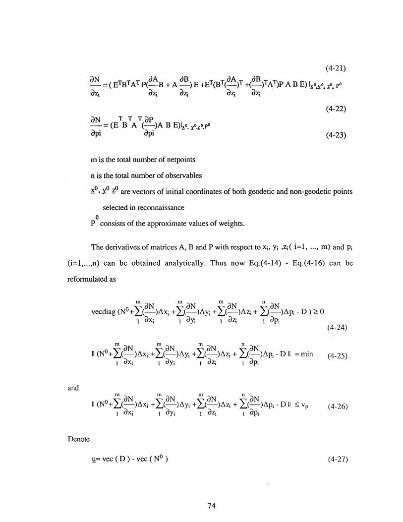
(4-21)
oN =(ETBTATP(oAB+A oB)E+ET(BT(oA)T +(oB)TAT)PABE)I~o..xo£~£pO 021 021 021 021 021 .
(4-22) oN T T ToP - = (E B A (-)A B E)l.!o. :xo~o,po opi opi (4-23)
m is the total number of netpoints
n is the total number of obsezvables
~0 ' tJ.tJ are vectors of initial coordinates of both geodetic and non-geodetic points
selected in reconnaissance 0
P consists of the approximate values of weights.
the derivatives of matrices A, Band P with respectto Xi, Yi ,zi( i=l, ... , m) and Pi
(i=l, ... ,n) can be obtained analytically. Thus now Eq.(4-14) - Eq.(4-16) can be
reformulated as
(4-25)
and
(4-26)
Denote
y= vee ( D ) - vee ( N° ) (4-27)
74
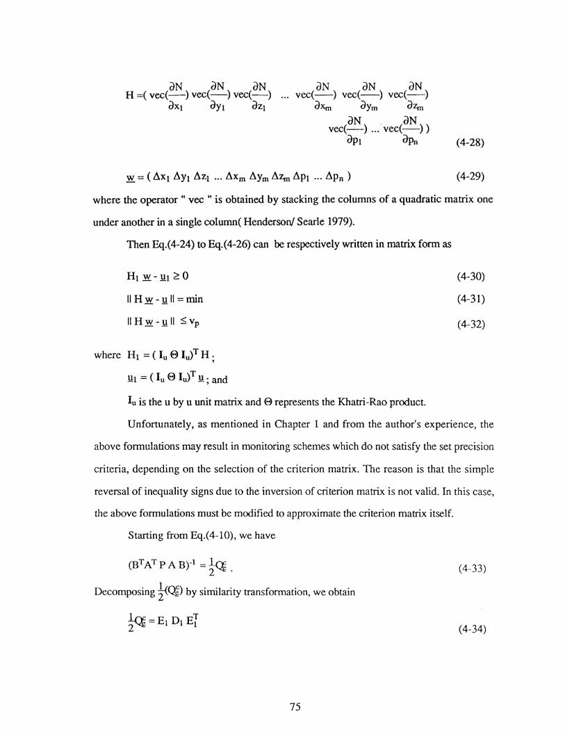
aN aN aN H =(vee(-) vee(-) vee(-)
axl an azl aN aN aN
vee(-) vee(-) vee(-) aXm aym d1ffi
aN , aN vee(-) ... vee(-) )
ap1 aPn (4-28)
(4-29)
where the operator " vee " is obtained by stacking the columns of a quadratic matrix one
under another in a single column( Henderson/ Searle 1979).
Then Eq.(4-24) to Eq.(4-26) can be respectively written in matrix form as
IIHw-yll=min
II Hw-yll ~vp
where Ht = ( lu E> lu)T H. ,
(4-30)
(4-31)
(4-32)
luis the u by u unit matrix and E> represents the Khatri-Rao product.
Unfortunately, as mentioned in Chapter 1 and from the author's experience, the
above formulations may result in monitoring schemes which do not satisfy the set precision
criteria, depending on the selection of the criterion matrix. The reason is that the simple
reversal of inequality signs due to the inversion of criterion matrix is not valid. In this case,
the above formulations must be modified to approximate the criterion matrix itself.
Starting from Eq.(4-10), we have
(BTAT p A Btl =In: 2'4;.
Decomposing !"<~) by similarity transformation, we obtain
75
(4-33)
(4-34)

with E1 and D1 the orthonormal matrix consisting of the normalized eigenvectors of!<~)
and the eigenvalues of -}<qg) respectively. And it can be shown that
E1 =E
Dt =D-1.
In this case, Eq.(4-33) changes to
ET (BTATP A B)-1 Et =Dt.
Denoting Nt = BTAT P A B,
and approximating N 1 by Taylor series of linear form, we have
0 m, n, ~.0, y_0 tJ, and p mean the same as before.
76
(4-35)
(4-36)
(4-37)
(4-38)
(4-39)
(4-40)
(4-41)
(4-42)
(4-43)
(4-44)

The inverse of the nonnal equation matrix N 1 can be expressed as:
(4-45)
Here, the first term on the right hand side of the equation may again be approximated by
applying the Neumann series restricted to linear tenn as:
[ ~ -tdNt ~ -tdNt ~ -1dN1 ~ -1dN1 ] = I- .LJ N0 --ilxi- .LJ N0 --ilyi- .LJ N0 --ilz;.- .LJ N0 ~Pi 1 dXi 1 dYi 1 dz;_ 1 dpi .
(4-46)
Finally, we get
(4-47)
And Eq.(4-37) leads to
(4-48)
Now, another set of formulations in regard to the precision criteria can be obtained as:
77

Hu w - .!!11 ::;; .Q
II H1 w - .!!1 1!. = min
II H1 w - !!1 1!.::;; Vp
where !!1 =vee <D1) - vee (ET <Nil )E1
!!11 = ( luE> lu )T !!1
T -1 dNt -1 Nzi = E1 N0 --N0 E1 ( i=l, · · ·, m) dZi
T -1 dN1 -1 Npi = E1 N0 --N0 E1 ( i=l, · · ·, n)
dPi
luis the u by u unit matrix and E> represents the Khatri-Rao product.
4.3.2 Internal reliability requirement
(4-49)
(4-50)
(4-51)
(4-52)
(4-53)
(4-54)
(4-55)
(4-56)
(4-57)
(4-58)
(4-59)
Traditionally, the internal reliability criterion works for the geodetic monitoring network
only. However, if in some cases the geotechnical instruments provide for geometric loop
closures or other redundancies, a similar treatment can be made. From Chapter 3, a general
internal reliability criterion for optimization can be
llrll =max (optimal internal reliability) (4-60)
or
78

llrll ~r1 (internal reliability control) (4-61)
where the redundancy numbers ri are defined as
1J. = ( I - Ao( A6 Po Aot1 A{; Po) i i. (i=1, ... , no) (4-62)
Replacing oij(A[; Po Ao)-1 by the criterion matrix of coordinates oij Qi, we have
Ti = ( 1- AoQiA{;Po) i i. (4-63)
Note that ri are nonlinear functions of coordinates but linear functions of weights. The
Taylor series expansion ofri can be expressed as
(4-64)
(4-65)
(4-66)
(4-67)
(4-68)
(4-69)
~can be obtained by Eq.(3-40) and (3-41) if the criterion matrix of deformation
parameters has been defined. Alternatively, it can also be approximated by
79

In this case, the above derivatives Eq.(4-66)- Eq.(4-69) can be reformulated as
(4-70)
(4-71)
(4-72)
(4-73)
(4-74)
(4-75)
(4-76)
(4-77)
(4-78)
(4-79)
(4-80)
(4-81)
Finally, if written in vector form, thevectorr= (r1 r2 ... rno )T can be expressed as
80
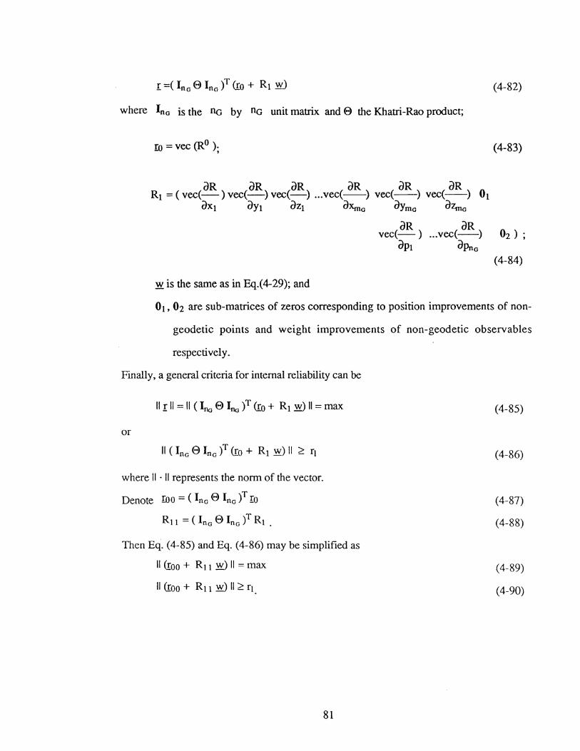
(4-82)
where Ina is the no by no unit matrix and 8 the Khatri-Rao product;
ro = vee (R0 ). '
(4-83)
aR aR aR aR aR aR R1 = (vee(-) vee(-) vee(-) ... vee(--) vee(--) vee(--) 01
dXt dYl dZt dXm.0 dYmo dZm0
aR aR vee(- ) ... vee(-) 02 ) ;
dPt dPno (4-84)
w is the same as in Eq.(4-29); and
01, 02 are sub-matrices of zeros corresponding to position improvements of non-
geodetic points and weight improvements of non-geodetic observables
respectively.
Finally, a general criteria for internal reliability can be
llrii=II(IIIGS~)T<ro+ Rtmll=max
or
where II · II represents the norm of the vector.
Denote roo= (Ina 8 Ina )T !o
R11 = (Ina 8 Ina f Rt .
Then Eq. ( 4-85) and Eq. ( 4-86) may be simplified as
II <roo + R11 W II =max
II <roo+ R11 Y!) II~ rt
81
(4-85)
(4-86)
(4-87)
(4-88)
( 4-89)
(4-90)

4.3.3 External reliability criteria
In the consideration of external reliability, only the influences of gross errors in
geodetic observations on the solution of deformation parameters will be considered here.
However, the formulations developed below can be easily extended to include also the
influences of gross errors in non-geodetic observations. From Chapter 3, a general external
reliability criteria for the estimation of deformation parameters can be
II A_ II =min {optimal external reliability) (4-91)
or
(external reliability control) (4-92)
where Am is the given maximum allowable value and
(4-93)
Here again, A o. i (i=l, ... , no) are nonlinear functions of positions but linear functions of
weights. Using Taylor series expansion, we have
(4-94)
where
(4-95)
(4-97)
82

(4-98)
(4-99)
Again, if written in vector form, the vector A. = ( A o, 1 A o, 2 ••• A o, no ) T can be expressed as
2 ~ =00 rno( Ina 8 Ina )T {go+ Gt W
where Ina is the no by no unit matrix and 8 the Khatri-Rao product. '
go =vee (0°)
ao ao ao ao ao ao G1 = (vee(-) vee(-) vee(-) ... vee(-) vee(-) vee(-)
OXt OYt OZt OXm OYm ozm aa aa
vee(- ) ... vee(-) ) opt aPn
w is the same as in Eq.(4-29).
Thus, a general criteria for external reliability can be
or
where II · II represents the norm of the vector.
let !!OO = ( Ino 8 Ino )T go
Gtt = ( In0 8 Ino )T Gt .
Then Eq. (4-103) to (4-104) may be written more compactly as
II (goo+ G11 .Yi) II= min
and
83
(4-100)
(4-101)
(4-102)
(4-103)
(4-104)
(4-105)
(4-106)
(4-107)
(4-108)
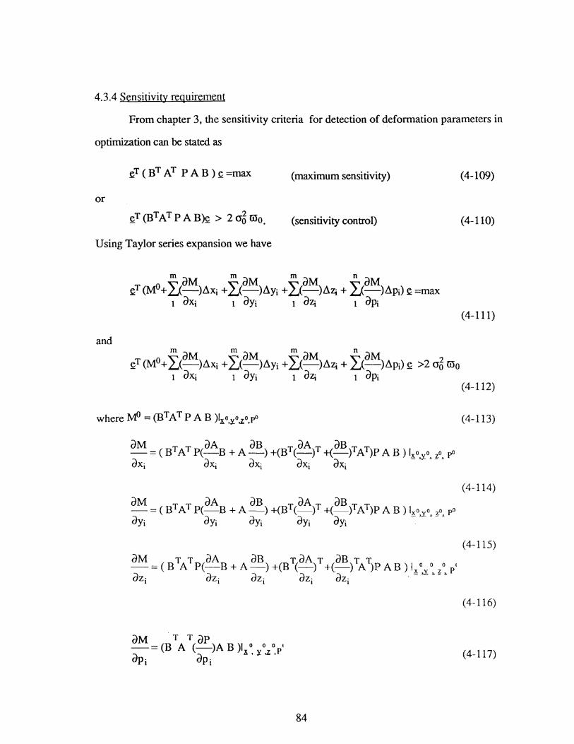
4.3.4 Sensitivity requirement
From chapter 3, the sensitivity criteria for detection of deformation parameters in
optimization can be stated as
(maximum sensitivity) (4-109)
or
(sensitivity control) (4-110)
Using Taylor series expansion we have
m dM m dM m dM n dM !.!T {MJ+ ll-)Axi + ll-)Ayi + ll-)Azt + ll-)APi)!.! =max
1 dXi 1 dYi 1 dz;_ 1 dPi (4-111)
and
(4-113)
(4-114)
(4-116)
(4-117)
84

Let T 0
s 0 =~ M ~ (4-118)
aM aM k~Mk aM aM aM ~=(kT_k kT_k kT __ k kT_k kT_k
axl ay1 azl aXm aym a21n
aM ~T-~
aM ~T-~ ) (4-119)
aP1 aPn
Then Eq:( 4-111) to Eq.(4-112) reduce to
so+ .s.Tw= max (4-120)
or
(4-121)
where w is the same as in Eq.(4-29), and
(4-122)
4.3.5 Cost requirement
A simplified cost criterion for optimization can be
IIPII= min (minimum cost) (4-123)
or
IIPII~ Cm (cost control) (4-124)
where P is the weight matrix of observations and II · II represents the norm of a matrix.
When using Taylor series expansion, matrix P can be expressed as
(4-125)
where pO is the approximate weight matrix. Considering P is a diagonal matrix, we have
II P II = II vecdiag (P) II n aP
=II (In e In )T (vec(pO) + I vee(- ).1.pj) II apj
(4-126)
85

Thus Eq.(4-123) to Eq.(4-124) can be reformulated as
ll£oo + C 11 w II= min (4-127)
or
(4-128)
where
(4-129)
(4-130)
w is the same as in Eq.(4-29);
In is then by n unit matrix and e the Khatri-Rao product; and
0 is the sub-matrix of zeros corresponding to position improvements.
4.3.6 Physical constraints
(a) Datum consideration
Since a translation, rotation and scaling of the monitoring scheme does not change
the shape of the scheme, the position improvements to be introduced for the netpoints
should be constrained such that no translation, scalling and differential rotation with respect
to the scheme to be optimized are introduced i.e.
(4-131)
where oT =( DJ oT) with De the datum matrix used to calculate the coordinates of
netpoints; 0 is a sub-matrix of zeros corresponding to weight improvements; and w is the
same as in Eq.(4-29).
86

(b) Realizability
At first, the position improvements to be introduced should be bounded by the
topography and/or other considerations, i.e.
bt iS Ayi S b2 i
c1 i S AZi S c2 i
(i= 1, ... , m) (4-132)
where the boundary values [ a1 i , a2 J , [bi i ' b2 J , and [ c1 i ' c2 J may be established in
the field by reconnaissance.
As for the weight changes APi (i=1, ... , n) to be introduced, the weights of
observations should be non-negative and be bounded by the maximum achievable accuracy
of the available instruments, i.e.,
(4-133)
or
0 ~ 0 -pi S Api S 2 -Pi =(Apikax (O'i)min
(i=l, ... , n) (4-134)
where PP (i=1, ... , n) are the approximate values for weights Pi
ifo is the a priori variance factor; and
(ai)~in (i=l, ... , n) are the minimum variance which can be achieved for each
observable li (i=l, ... , n).
Combining Eq.(4-132) and Eq.(4-134) and written in matrix form we have
Aoo w Shoo
where Aoo = r-II) with I the (3m+n) by (3m+n) unit matrix; and
boo= (a21 b21 C21 ... a2m ~ C2m (Apt)max ... (APn)max.
-an -bn - Cn ... -alm -blm -Clm P? ... p~ )T.
87
(4-135)
(4-136)
(4-137)

4.4 Formulation of Mathematical Models for Optimization
Mathematically, optimization means determining the maximum or minimum of a
target function under a number of constraints ( equalities or inequalities or both ). For our
purpose -- the optimization of a monitoring scheme, the target function will be one which
represent the quality of the monitoring scheme. As discussed before, the four general
measures used to evaluate this quality are precision, reliability, sensitivity and economy. A
monitoring scheme should be designed in such a way that it can realize the required
precision of the deformation parameters; can be resistant to gross errors in the observations
and minimize the effects of undetected gross errors on deformation parameters; can allow
testing of special hypothesis with higher significance; and can satisfy certain cost limit
Therefore, from the suggestion of Schaffrin (1985), our target function will be of the type:
<Xp (precision)+ O.r (reliability)+ O.s (sensitivity)+ O.c (cost )-1 =max (4-138)
for suitably chosen weight coefficients a.p, O.n O.s, and O.c • This is a multi-objective
optimization problem. If we let one of the coefficients go to infinity, we obtain some
extreme cases of the target function (Schaffrin, 1985):
Case (1): O.c --> oo ==>cost= min
precision ~ constant
reliability ~ constant
sensitivity~ constant
Here the cost is optimized while we have to control the precision, reliability,
and sensitivity.
Case (2): O.p --> oo ==>precision= max
reliability ~ constant
sensitivity ~ constant
cost ~ constant
88

Here the precision is optimized while we have to control reliability, sensitivity,
and cost.
Case (3): <Xr --> oo ==> reliability = max
precision ~ constant
sensitivity ~ constant
cost :5; constant
Here the reliability is optimized while cost, precision, and sensitivity are
controlled.
Case ( 4): <ls --> oo ==> sensitivity = max
precision ~ constant
reliability ~ constant
cost :5; constant
Here the sensitivity is optimized while precision, reliability, and cost are
controlled.
Thus, depending on which alternative we choose, the mathematical models for the
optimization of a monitoring scheme can be established by combining a number of the basic
requirements out of the ones discussed in the above section.
Model 1: Best approximation of the criterion matrix
II H w - !! II = min
Subject to: H1 w- !!1 ~ 0
II <roo + R11 W II ~ r1
II (goo + G11 w) II ~ Am
11 .9>0 + C 11 W 11:5; Cm
SO+ ~Tw >Sm
nTw=O
Aoo w :5; hoo
89
(I-1)
(I-2)
(I-3)
(I-4)
(I-5)
(I-6)
(I-7)

Model II: Maximizing the internal reliability
- II <roo + R11 ~ II =min
Subject to: Ht w- !!1;;::: 0 (II-1)
II H w -!! II $; Vp (II-2)
II {goo + Gu ~ II ~Am (II-3)
li9Jo + C 11 w II~ Cm (II-4)
SO+ :iTW >Sm. (II-5)
nTw=O (II-6)
Aoo w ~hoo (II-7)
Model III: Maximizing the external reliability
II <zoo + G11 W II =min
Subject to: H1 w- !!1;;::: 0 (III-1)
II H w-!! II ~ Vp (111-2)
II Croo + Ru w II ~ r1 (111-3)
11 910 + C 11 W II~ Cm (III-4)
SO+ :iT W >Sm (III-5)
nTw=O (111-6)
Aoo w ~hoo (111-7)
90

Model IV: Maxjmjzine the sensitivity
-(so + ~T Yi. )= min
Subject to: H1 w- .Y.1 ~ 0 (IV-1)
II H w - yll !5; Vp (IV-2)
II <roo + R11 W II ~ r1 (IV-3)
II {goo + Gu ro II !5; Am (IV-4)
11 9>0 + C 11 W 11!5; Cm (IV-5)
nTw=O (IV-6)
Aoo w !5; .b.oo (IV-7)
Model V: Minimizine the cost of observations
11 £oo + C 11 w II = min
Subject to: H1 w- !!1 ~ 0 (V-1)
II H w - !! II !5; Vp (V-2)
II <roo + R11 W II ~ r1 (V-3)
II {goo + Gu ro II !5; Am (V-4)
SO+ ~T W >Sm (V-5)
nTw=O (V-6)
Aoo w !5; .b.oo (V-7)
91
4.5 Solution of the Mathematical Models
4.5.1 The choice of norm
Up to now, the mathematical models for the optimization of a monitoring scheme
have been established except that all the norms of matrices and vectors in the models were
not defined. Depending on the choice of norm, the whole problem gets a different
formulation and, as a consequence, we have to apply a different algorithm in order to find
its solution. If, for instance, we allow for general norms within the models, we would
obtain general mathematical programming problems with linear and non-linear constraints.
A mapping of a linear vector space :X over 1R. into 1R. is called "norm", and its
value for~ e :X is denoted by II ~ II, iff it holds:
(1) II ~ II ~ 0 for~ e :X
(2) ll~+yll~ ll~ll+llyll for~. ye :X
(3) II a. ~ II = la.l II ~ II for ~ e :X, a. e lR
(4) I X II =0 ==> ~=0 .
A "matrix norm" can be defined in terms of a vector norm. Given a vector norm II · II and a
matrix A, consider II Ax II for all vectors such that II~ II =1. The matrix norm induced by
the vector norm is given by
flAil= max IIA~II 11~11=1
(4-139)
Typical examples are the IP- norms for finite dimensional vector spaces as defined with
respect to some algebraic basis by
(4-140)
for any arbitrary chosen number p with 1~ p ~ oo. For p =1,2, and oo, the
11-norm , 12 -norm, and 100-norm are defined respectively as
92

n
II ( X 1, X 2, .. . , Xn) ll1 = L I Xi I 1
~ 2 l/2 II ( x 1, x 2, ••. , xn) 11 2 = ( Li xi )
1
ll(x1,X2, ... , Xn)lloo =max{lxi I, i=1, ..• , n)
The 100-norm is also called " uniform norm" or " Tschebycheff norm".
(4-141)
(4-142)
(4-143)
On the other hand, for any space of matrices with arbitrary, but specified size we
may obtain a matrix norm simply by identifying
II A II = II vee (A) II (4-144)
for a certain vector norm, where the "vee" operator stacks one column of the matrix under
the other.
As for the "choice of norm" for network optimization, it has been argued by
Schaffrin (1981) that a choice of p with 1~ p<2 would be less suitable for fitting a criterion
matrix because of the loss of smoothing power while for cost requirement p should not
exceed 2. Van Mierlo"(l981) suggested 100-norm for reliability. Therefore, as a typical case,
we will use 12-norm, 11-norm, and 100-norm for the best fitting of the criterion matrix, for
the minimum cost, and for the maximum reliability requirements respectively. And use 1
1 -norm for precision control Eq.(4-32). Under these considerations, the above proposed
mathematical m<Xiels <n to (V) become:
93

Model 1: Best approximation of the criterion matrix
Minimize ( w T HT H w - 2!! T H w + .Y. T !!)
Subject to: H1 w- 111 ~ 0 (1-1)
<roo + R11 .W ~ n (1-2)
{goo + G11 .W ~ Am (1-3)
'J.T 9>0 +'J.T C 11 W ~ Cm (1-4)
SO+ ~Tw>Sm (1-"5)
nTw=O (1-6)
Aoo w ~ .b.oo (1-7)
where "i. is a (3m+n) by 1 vector of constants;
n is the I1G by 1 vector with all elements being I'J.;
Am is the IlG by 1 vector with all elements being Am.
Model II: Maximizin1: the internal reliability
Minimize max { - Croo + R11 Wi ,i=1, ... ,na}
Subject to: H1 w- 111 ~ 0 (11-1)
-v ~Hw-u~ v ..!..p - - -P (11-2)
(goo + G11 .W ~ .&n (11-3)
"i.T 9>0 +'J.T C 11 W ~ Cm (11-4)
SO+ ~Tw >Sm (11-5)
oTw=O (11-6)
Aoo w ~.2oo (11-7)
where Yp is a u2 by 1 vector with all elements being Yp.
94

Model III: Maximizing the external reliability
Minimize max { (goo+ Gu ~i , i =1, ... , no}
Subject to: Ht w- .Yt ~ 0 (111-1)
-Yp~Hw-y~ Yp (ll-2)
<roo + Ru w ~ n (ll-3)
·:l9>o +'J.T C 11 w ~ Cm (111-4)
SO+ ~Tw>Sm (111-5)
nTw=O (111-6)
Aoo w ~hoo (111-7)
Model IV: Maximizing the sensitivity
so+ .s.T w = max
Subject to: H1 w- !!1 ~ 0 (IV-1)
-Yp ~Hw-y~ Yp (IV-2)
<roo + Ru w ~ n (IV-3)
{goo + Gu w ~ &n (IV-4)
;l 9>0 +'J.T C 11 W ~ Cm (IV-5)
nTw=O (IV-6)
Aoo w ~hoo (IV-7)
95

Model V: Minimizing the cost of observations
Minimize 'l9>o +':t.T C 11 w
Subject to: H1 w- .!.!1 ~ 0 (V-1)
-Yp~Hw-y~ Yp (V-2)
<roo + Ru .W ~ n (V-3)
{goo + Gu .W ~ &n (V-4)
SO+ ~Tw>Sm (V-5)
oTw=O (V-6)
Aoo w ~D.oo (V-7)
4.5.2 The Solution methods
As is clear from the above discussion. obtaining the solutions of the above
mathematical models can be summarized as solving one of the following standardized
approximation problems with linear equality or inequality constraints:
(1) 11 -approximation
Minimize II M w- f ll1
Subject to En w ~ fu
(2) 12-approximation
Minimize II M w - f 1!2
Subject to E22 w ~ fn
(3) !""-approximation
Minimize II M w - f 1100
Subject to Eoo w ~ L
Model I is the 12-approximation solvable by Quadratic Programming (QP); Model II and
Model ill are the !""-approximation solvable by Dual Linear Programming (DLP) or by QP;
96

and finally Model IY and Model Y are the 11 -approximation solvable by linear
programming (LP). Standard software for Linear- or Quadratic Programming, if available,
can be used to obtain the solutions for the mathematical models. Also, Schaffiin (1981)
introduced the Linear Complementary Algorithm (LCA) or Parametric Linear
Complementary Algorithm (PLCA) to solve the QP or LP problems, since the former may
improve numerical stability and therefore are very efficient. The purpose of PLCA is to
allow the infeasible constraints to be transformed into feasible ones by introducing
additional parameters. Basic theories of QP, LP, and LCA will be discussed in appendix II.
4.6 Analysis of Solvability and the Multi-Objective
Optimization MOdel (MQQM)
4.6.1 The Concept of Multi-Objective Optimization
The study of the multi-objective optimization is a well established branch in
operations research. The mathematical theories involved are quite sophisticated. In the
following a brief explanation of the problem statement and the solution concepts is given in
order to apply this theory to solving our problems.
A Multi-Objective Optimization Problem (MOOP) is defined as:
Minimize f(K) = (ft (x), ... , fp{K))T
Subject to K EX = (K: g(K) = (gtU), ... , gmU))T s; 0 }
where fi (i=l; ... , p) are the individual objective functions and gj (j=l, ... , m) the
constraint functions. Here all the functions are assumed to be continuously differentiable.
This kind of problem is also called a vector optimization.
Unlike traditional mathematical programming with a single objective function, an
optimal solution that minimizes all the objective functions simultaneously does not
necessarily exist. The final decision should be made by taking the total balance of
97

objectives into account. Thus the decision maker's value is usually represented by saying
whether or not an alternative~ is preferred to another alternative x', or equivalently whether
or not f(x) is preferred to f(x'). For this purpose, a scalar-valued function u(ft. · · ·,fp)
representing the decision maker's preference called preference function has to be defined.
Once we obtain such a preference function, our problem reduces to the traditional
mathematical programming:
Maximize u(ft. · · ·,fp)
Subject to 2£ eX= {t£: g(K) = (gt (2£), •.. , gm W)T ~ 0 } .
Instead of strict optimality, the notion of efficiency is introduced in multi-objective
optimization. A vector f® is said to be efficient if there is no fW <2£ e X) preferred to f®.
Mathematically, the most fundamental kind of efficient solution is usually called a Pareto
optimal solution or noninferior solution. A point x EX is said to be a Pareto optimal
solution( or noninferior solution) to the problem MOOP if there is no x EX such that
fW::; f@. The final decision is usually made among the set of efficient solutions. There
are a number of ways to characterize the efficiency of a solution. One characterization is
taken as the best approximations to the ideal point. Consider the multi-objective
optimization problem MOOP, an ideal point f = <ft • · · ·, fp)T is defined as:
fi = inf{fiW: X eX} > -oo, i=l, · · ·, P. (4-145)
However, we might take another ideal point f as f::; f. A solution i is efficient if
d = II f(X) - f II = inf{ llfW - f II } X E X ( 4-146)
where II · II represents the norm of a vector. It can be the lp -norms as defined by
(4-147)
or the one introduced by Dinkelbach and Iserrnann(1973)
98

p
II flip =II flloo + j_ (L I J.li fil ), p e [1, oo) p i=l
(4-148)
where J! = (JJ.t. J.12, · • ·, J.lp )T is the weighting vector. Intuitively, if the ideal point is
unattainable, d=llfW - f II represents the distance between fW and f and can be considered
as a measure of regret resulted from unattainability of fW to f . An efficient solution is to
minimize this regret. In order to apply this idea in practice, the following problems have to
be solved:
(i) How to choose the distance function?
(ii) How to decide the weighting vector? and
(iii) How to make a common scale for the different objective functions?
At first. Sawaragi et. al. (1985) suggests that it suffices to use the lp -norms with p ~ 1 to
evaluate the distance. The solution to problem (ii) is quite subjective, since that is closely
related to the decision maker's preference attitudes to some specific objective functions.
Thus, one used to adopt the weight based on his experience. If the same weight is selected
for each objective function, then the resulting solution is the one that improves equally. in
some sense, each criterion as much as possible. Dyer(1972) suggested a numerical method
for deciding the weights under interaction with decision makers. The method is complicated
and difficult to use in practice. Finally, if the lp -norms distance function is used, it is
important to make a common scale for the objective functions. For example, if the positive
and negative values of the objective functions are mixed, or if their physical units and
numerical orders are different from each other, then some of the objective functions are
sensitive and others not. One approach to make a common scale for objective functions is
to use the relative degree of the non-attainability of fi(x) to the ideal value fi 1.e.
(fiW- fi)/fi as new objective functions. This enables us to ignore the need to pay extra
attention to the difference among the dimension and the numerical order of the different
objective functions.
99

4.6.2 The Multi-Objective Optimization Model (MQQM) for Monitoring schemes
In the above sections, the mathematical models for the optimization of a monitoring
scheme have been established. For practical applications, depending on the aspects of the
problem we prefer, we may choose one of the formulations Models I to V to obtain the
optimal configuration and observation plan of a monitoring scheme. Since the objective
function in Model I is strictly convex for a positive-definite matrix HTH, it has a unique
minimizing solution if and only if the constraints in Eq.(l-1) to Eq.(I-7) are consistent. In
Models II to V, the objective function are convex, they have unique minimizing solutions if
and only if their respective constraints in Eq.(i-1) to Eq.(i-7) (i=II, III, IV, V) are
consistent and no rank deficiency exists for the coefficient matrix of the whole set of
constraints of each model. Therefore, the consistency of constraints is decisive for the
solution of each of the mathematical models. The possibility of inconsistency of constraints
in Eq.(l-1) was discussed by Schaffrin (1980). He proposed to approach the inconsistency
by "parameterization" i.e. by adding a certain negative value at the right hand side in order
to generate consistency and thus the existence of the desired solution. The problem with
that approach is that through the "parameterization", the original constraints in Eq.(I-1)
become in fact redundant.
An analysis of the constraints in Eq.(I-1) to Eq.(I-7) indicates that the physical
constraints in Eq.(I-6) to Eq.(I-7) are compulsory. They represent the physical
environment in which we can optimize our monitoring scheme. In most cases, the
precision, reliability, sensitivity and cost constraints (Eq.(I-1) to Eq.(I-5)) may be
contradictory, i.e., the best monitoring scheme simultaneously which would satisfy the
objective function and all the constraints may not exist. That can be understood in this way:
once the maximum precision of instrumentation, the total expenditure, and the topographic
conditions are given, the maximum precision, reliability, and sensitivity attainable are
limited. Thus if the criterion matrix of deformation parameters <io Qg, the criterion vector
for internal and external reliability n ... &n, and the criterion number for sensitivity Sm, are
100

not defined properly, i.e. if they exceed the reality, then the constraints in Eq.(I-1) to
Eq.(l-5) will be inconsistent, and no solution exists. This analysis is applicable to all the
other four Models II to V. Therefore, to ensure a universally applicable optimization
procedure, a unified mathematical model, called the Multi-Objective Optimization Model
(MOOM), is proposed, in which instead of approximating the constraints in Eq.(l-1) to
Eq.(l-5) "from one side", an approximation "from both sides" is permitted. The point is to
minimize the differences between the precision, reliability, sensitivity, cost and their
respective ideal counterparts simultaneously, subject to the physical constraints. This model
includes all the intentions of Models I to V, and can be described as:
Minimize II H Y!. -!! II + II Rtt Y!. -( n -roo) II 1 II G11 Y!. -( .lian-goo) II + II y II II n - roo II l!Am-gooll
+II yT C 11 Y!. -(em- yT ~o) II +II ~T Y:!..- (Sm-so )II
II Cm- yT £oo 1! II Sm-SO II (4-149)
Subject to: D T w = 0
Aoo w ~boo. (4-150)
By applying 12 - norm from the point of view of computational benefit, the above model
may be simplified as
where
Mi · · (wTU'!'How-2uTHow+uTnn) mrruze - ... .o.u - .!!0 - .!!0 ~
Subject to: nT w = 0
Aoo w ~boo
H/YyTy
Ru /-../yJyl
Ho = G11 I ,.f!{fi; yT c11 1 ~u3· u3
~TI~lJ4· \Lt
yiYyTy_
!!1 I -J !!T!!t
!!o = !12 I ,.f!{fi;
101
u3 I ~u3· u3
141~14'14
(4-151)
(4-152)
(4-153)

lll = n- roo
1!2 = And~OO
U3 = Cm - 'i.T 9>0
114 = Sm-So.
In fact, this mathematical model corresponds to the solution of the multi-objective
optimization problem(Eq.(4-138)) under the concept of "ideal point" with specified "ideal
point" representing precision, internal and external reliability, sensitivity and cost being Y....
(n- roo), <Am- goo), !Crn -'i.T £oo), (Sm- so) respectively. Interpreting this intuitively,
this model tries to best approximate equally the precision, reliability, sensitivity, and cost
criteria under the given geography and instrumentation condition in the sense of least
squares. If an appropriate weighting vector!!= (<Xpre.• <Xirelia.,(lerelia. <lsens.• <lcos. )T with
elements for precision, internal reliability, external reliability, sensitivity, and cost
respectively is selected, the selection of which is based on the specific problems to be
solved and to a large extent subjective, then the decision maker desires to improve some of
the criteria with larger weights more strongly than the others. This practical meaning
encourages us to accept easily the obtained solution. This model has a unique minimizing
solution if and only if the matrix HJ'Ho is positive definite. For practical applications, some
of the quality criteria may be omitted in the objective function. In this case the model tries to
best approximate the ones which appear in it. The rule which governs the solution does not
change.
However, if there is a case where all the design criteria of precision, reliability, and
sensitivity must be satisfied whatever the total expenditure of the project is, then the above
mathematical model must be modified by approximating the design criteria "from one side",
I.e.
102

Minimize ~Tfl60Hoow- 2.YJoHoow + !!&'o!!Oo) (4-154)
Subject to Au~~ Qll
DTw=O (4-155)
Aoow ~!roo
where
Ht/../yflh· ytf.../ yfyl
-Rttl..f YIY.2 Y.2t...f Y.IY.2
Hoo= Glt/.../yJYJ YOO = YJ/.../yJYJ (4-156)
·:l CuNll4 ~ 114 U4rr;;;;:;;; -~ T t-J Uy Us us,..r;;;:;;;
Hu
-R11
( YH ) A11 =
blt= ~ (4-157)
Gn
-§T
H1, Y1 , and H11. !!11 are defined in Eq. (4-49) and (4-50);
Y2 =roo- II;
Y3 = Am -goo· ,
ll4 = Cm -yT ~o; and
US= so- Sm.
This model will result in a monitoring scheme in which the achievable precision, reliability,
and sensitivity will be better or at least equal to the specified values. However, here the
upper limits regarding the weights in vector boo have to be put large enough so that all the
constraints are feasible.
It should be noted that all the solutions to the above mathematical models should be
iterative since Taylor series of linear form is used. A Fortran-77 computer program using
Quadratic Programming to solve the above proposed mathematical models was completed
by the author. The simulation study and its applications will be discussed in Chapter 5.
103

4.7 Summary of the Optimization Procedures
~· Identification of the deformation parameters to be detected.
First of all, to establish a monitoring scheme, one has to clearly
know the purpose it is to serve, i.e., what kind of deformation parameters is
to be detected. At the design stage, the deformation model is usually not
fully understood. Therefore, except for the case where the deformation
model has been specified by the users or derived from previous
observations, the construction of the deformation model may be based on a
study of the relevant physical properties of the object and on the knowledge
of the acting forces (deterministic modelling).
~· Field reconnaissance
Once the purpose of the monitoring scheme is clarified, one has to
perform the field reconnaissance. The purpose of the reconnaissance is to
select locations for both geodetic and non-geodetic survey points; and to
determine all possible types of both geodetic and non-geodetic instruments
which would be suitable for the detection of the expected deformations.
Then the approximate coordinates of the selected survey points are
determined in an appropriate local coordinate system. The possible
coordinate changes to be introduced for the initially selected survey points
may also be determined from the topography and/or other conditions.
~· Definition of the design criteria
The design criteria include precision, reliability, sensitivity, and
economy. The methodology for the determination of these criteria is
described in Chapter 3.
104
Step 4. Solution of the optimal configuration and observational weights of the
monitoring scheme
The optimal configuration and observational weights of the
monitoring scheme can now be solved for using the methodology developed
in Chapter 4. The solution gives the optimal coordinate changes to be
introduced to the initially selected survey points and optimal weight changes
to be introduced to the initially adopted approximate weights. The selection
of the initial weights may be arbitrary. Therefore, the optimal values of both
coordinates and weights are obtained by adding the optimal changes, as
obtained from the solution, to their corresponding approximate values.
~· Finalization of the monitoring configuration and observation plan
The survey marks can now be monumented according to the solved
optimal coordinates of all the initially selected points. As far as the
observation scheme is concerned, all the observables which from the
optimization in Step 4 obtained zero or close to zero weights can be
eliminated from the final design of the monitoring scheme. Check the design
criteria to make sure that all the criteria have been satisfied.
Figure 4.2 shows the computation flowchart.
105
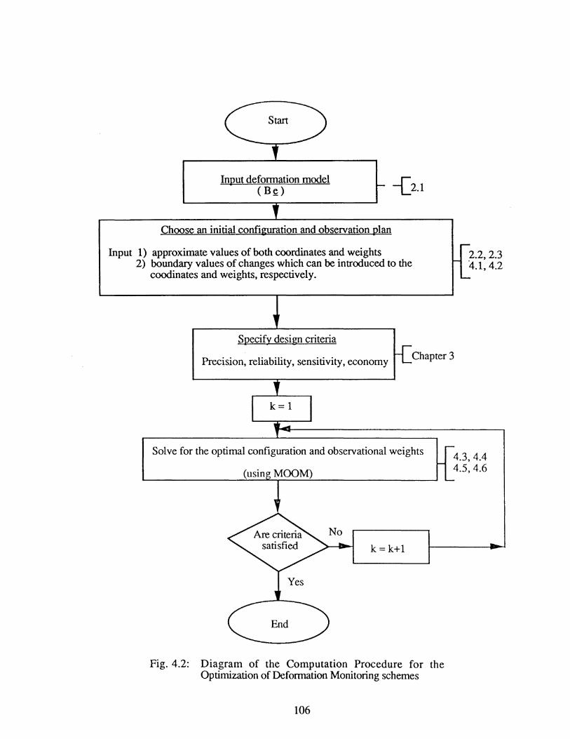
Input defonnation model ( B~)
Choose an initial configuration and observation plan
Input 1) approximate values of both coordinates and weights
-[2.1
2) boundary values of changes which can be introduced to the coodinates and weights, respectively.
Specify design criteria
Precision, reliability, sensitivity, economy Chapter 3
Solve for the optimal configuration and observational weights
(usin MOOM)
k=k+1
Fig. 4.2: Diagram of the Computation Procedure for the Optimization of Defonnation Monitoring schemes
106


CHAPTERS
SIMULATION STUDIES AND OPTIMIZATION EXAMPLES
5.1 Simulation Studies
In order to test the validity of the above developed methodology, simulation studies
have been performed using two examples. The simulated example No. 1 confirms the
correctness of the developed mathematical model MOOM. Simulation study No. 2
illustrates the significance of applying relatively small position changes of netpoints for the
optimal solution of observation weights.
5.1.1 Simulation study No. 1: verification of the correctness of the developed
mathematical models
Let us consider a simple monitoring scheme (Fig. 5.1) established for the purpose
of detecting creep between two tectonic blocks along fault and strain accumulation. This
scheme consists of a fault-crossing geodetic network plus some isolated strainmeters placed
near each of the geodetic stations with the same orientations of 45 degrees. The desired
coordinates of geodetic netpoints are listed in Table 5.1. The shortest and longest distances
of the network are 2.00 km and 3.61 km respectively.
Assuming the deformation model includes a relative rigid body translation between
Block II and Block I plus a homogeneous strain field over the whole area, it can be
expressed as
107

Table 5.1: Desired coordinates for the geodetic netpoints
Point
1
2
3
4
5
6
y
x (m)
500.00
500.00
2500.00
2500.00
5500.00
5500.00
y (m)
600.00
2600.00
600.00
2600.00
600.00
2600.00
;.
I l Block II i '
1 ~----,l'"""r--']-, ----~L'\. '
/'discontinuity f f
[ill Strainmeters
6. Geodetic points
Fig. 5.1: The simulated monitoring scheme
108
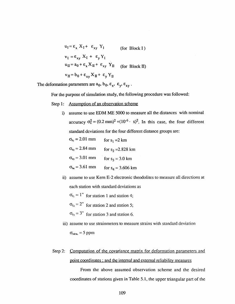
ul= Ex XI+ Exy YJ
v1 =Exy XI+ Ey y 1
(for Block I )
u II= ao + Ex X II+ Exy y II (for Block IT)
vii=b0 +ExyXII+ EY YII
The defonnation parameters are ao, ho, Ex, EY, Exy.
For the purpose of simulation study, the following procedure was followed:
Step 1: Assumption of an observation scheme
i) assume to use EDM ME 5000 to measure all the distances with nominal
accuracy a'f = (0.2 mm)2 +(10-6 · s)2• In this case, the four different
standard deviations for the four different distance groups are:
0'51 = 2.01 mm
0'52 = 2.84 mm
0'54 = 3.61 mm
for s1 =2 km
for s2 =2.828 km
for s3 = 3.0 km
for s4 = 3.606 km
ii) assume to use Kern E-2 electronic theodolites to measure all directions at
each station with standard deviations as
1" O'rt = for station 1 and station 4;
~f2 = 2" v for station 2 and station 5;
3" O'r3 = for station 3 and station 6.
iii) assume to use strainmeters to measure strains with standard deviation
O'stra. = 5 ppm
Step 2: Computation of the covariance matrix for deformation parameters and
point coordinates : and the internal and external reliability measures
From the above assumed observation scheme and the desired
coordinates of stations given in Table 5.1, the upper triangular part of the
109

c.~=
covariance matrix of the deformation parameters ce can be obtained from
mm2 Eq.(4-7) as (unit: mrn.2 for translations, and m2 for strains)
6.59 -030 -1.19 . 10·3 5.51. w-5 5.70- 10"5
32.07 6.53. w·5 -2.31· 10"3 1.00· 10-4
4=2· 4.04-10"7 -1.52. 10-8 -5.81· 10-8
Symmetric 4.05. 10"7 -1.29. 10-8
2.80- 10"7
Without loss of generality, the covariance matrix for point
coordinates of the geodetic monitoring network can be obtained by
assuming point 1 and point 2 fixed as (unit mm2):
3.55 2.13 -0.30 1.84 3.48 7.40 -0.19 7.40 10.08 -1.79 8.32 2.40 15.39 -1.68 15.44
3.58 -2.15 -0.21 -7.60 3.57 -7.58 10.01 1.86 15.88 -2.48 15.83
10.71 13.26 -1.21 12.86 65.91 -13.28 63.89
Synunetric 10.97 -13.65 65.76
These matrices Ce and Cx will be used as the criterion matrices for
deformation parameters and point coordinates respectively in the
following optimization procedure.
The vector I 1 of redundancy numbers representing internal reliability
and the vector Am for external reliability under the assumption of
a.o = J3o=0.05 (i.e. 8o = 3.61) are listed in Table 5.6 and Table 5.7
respectively. Here it should be noted that, to avoid the introduction of
station orientation parameters for direction measurements, all the
directions at each station are replaced by appropriate correlated angles.
110

Step 3: Application of the mathematical model MOOM
To test the proposed mathematical model, we assume that the
parameters to be optimized are the positions of geodetic points 4, 5 and 6
and the weights or standard deviations of all the above proposed
observables. The positions of all the other geodetic netpoints and
strainmeters are not supposed to change. The input approximate
coordinates of the netpoints 4, 5 and 6 are listed in Table 5.2 which are
obtained by purposely shifting certain values as given in Table 5.3 from
the desired coordinates listed in Table 5.1; the input initial weights are
Pi = 1.0 for all observables.
In order to use the mathematical model MOOM, Cc and Cx are used
as the criterion matrices for the deformation parameters and the point
coordinates, respectively; The vectors I 1 and 2k m are used as the boundary
values for internal and external reliability respectively. Assume the vector
of magnitude of deformation parameters (ao, bo, Ex, f:xy, and Ey) to be
detected is ~T = [16.00(mm) 40.0(mm) 4 ppm 4 ppm 4 ppm], then
the boundary value for sensitivity (Eq. (4-110)) is Sm = 663.3721. The
minimum cost criteria is not considered.
After using the proposed optimization procedure, a comparison of
the simulated values and the optimization results is given in Table 5.3 -
Table 5.7. From Table 5.3 we can see that the maximum difference
between simulated position shifts and the optimized position correction is
0.57 rn, and Table 5.4 - Table 5.7 indicate that the differences between
the simulated weights, standard deviations, internal and external reliability
measures and their corresponding optimized values are practically zero as
expected. Also, the optimization procedure gives the same value for
sensitivity criterion sm as specified before.
111

To check the goodness of fitting of the criterion matrix, the difference matrix
between the covariance matrix of deformation parameters as calculated from the optimized
values and the criterion matrix is listed as follows:
8.36· w-6 -3.38· 10-4 -2.40. w-7 1.19· w-7 7.03· w-8
-7.76· w-6 2.18· w-7 1.49· w-7 4.05· w-8
8.64· w-11 -3.39· w-11 -1.43· w-11
Symmenic -2.05· w-11 -1.24· w-12
1.52· w-12
An analysis of the above results indicates that by starting with a set of approximate
coordinates of geodetic points and weights of observables, and given the optimality criteria
for precision, reliability, and sensitivity, the developed optimization model MOOM can give
us their corresponding optimal values which are practically the same as their true values.
These results unbiguously confirm the correctness of the proposed mathematical model.
112

Table 5.2: The input approximate coordinates of geodetic netpoints
Point x (m) y (m)
1 500.00 600.00
2 500.00 2600.00
3 2500.00 600.00
4 2550.00 2690.00
5 5560.00 680.00
6 5570.00 2660.00
Table 5.3: Comparison between the simulated position shifts and the optimized position corrections
Simulated Optimized Point position position
shifts corrections
~Simu. (m) -~Opti. (m) ~s· -(- ~Op. unu. tJ.
~X 50.00 50.44 -0.44 4
ll.y 90.00 89.57 0.43
ll.x 60.00 60.44 -0.44 5
~y 80.00 79.43 0.57
~X 70.00 70.15 -0.15 6
~y 60.00 60.32 -0.32
113
)

Table 5.4: Comparison between the simulated weights and the optimized weights
Simulated Optimized Observables weights weights (psimu. - Popti)
(Psimu.) (Popti.)
1 - 2 0.24768 0.24770 -0.00002 1 - 3 0.24768 0.24770 -0.00002 1 - 4 0.12409 0.12410 -0.00001 2- 3 0.12409 0.12410 -0.00002
distances 2-4 0.24768 0.24770 -0.00002 3 - 4 0.24768 0.24770 -0.00002 3 - 5 0.11058 0.11060 -0.00002 3 - 6 0.07672 0.07672 0.00000 4-5 0.07672 0.07672 0.00000 4- 6 0.11058 0.11060 -0.00002 5 - 6 0.24768 0.24770 -0.00002
station 1 1.00000 1.00012 -0.00012 station 2 0.25000 0.24999 0.00001 station 3 0.11111 0.11105 0.00006
directions station 4 1.00000 1.00012 -0.00012 station 5 0.25000 0.24999 0.00001 station 6 0.11111 0.11105 0.00006 strain. 1 4.00000 3.99995 0.00005 strain. 2 4.00000 3.99995 0.00005 strain. 3 4.00000 3.99995 0.00005
strainmeters strain. 4 4.00000 3.99995 0.00005 strain. 5 4.00000 3.99995 0.00005 strain. 6 4.00000 3.99995 0.00005
114

Table 5.5: Comparison between the simulated standard deviations and the optimized values
Simulated Optimized Observables standard standard
deviations deviations ( asimu. - aOpti. (asimu.) (Cfopti.)
1 - 2 2.01(mm) 2.01(mm) 0.00 1 - 3 2.01(mm) 2.01(mm) 0.00 1 - 4 2.84(mm) 2.84(mm) 0.00 2- 3 2.84(mm) 2.84(mm) 0.00
distances 2-4 2.01(mm) 2.01(mm) 0.00 3- 4 2.01(mm) 2.01(mm) 0.00 3- 5 3.01(mm) 3.01(mm) 0.00 3- 6 3.61(mm) 3.61(mm) 0.00 4-5 3.61(mm) 3.61(mm) 0.00 4- 6 3.01(mm) 3.01(mm) 0.00 5-6 2.01(mm) 2.01(mm) 0.00
station 1 1.00" 1.00" 0.00 station 2 2.00" 2.00" 0.00 station 3 3.00" 3.00" 0.00
directions station 4 1.00" 1.00" 0.00 station 5 2.00" 2.00" 0.00 station 6 3.00" 3.00" 0.00 strain. 1 5 ppm 5 ppm 0.00 strain. 2 5 ppm 5 ppm 0.00 strain. 3 5 ppm 5 ppm 0.00
strainmeters strain. 4 5 ppm 5 ppm 0.00 strain. 5 5 ppm 5 ppm 0.00 strain. 6 5 ppm 5 ppm 0.00
115

Table 5.6: Goodness of fitting of the internal reliability
The The simulated optimized
redundancy redundancy <n-ri) Observables numbers numbers
(n) (Ir) 1 - 2 1.0000 1.0000 0.0000 1 - 3 0.1208 0.1208 0.0000 1 - 4 0.4238 0.4238 0.0000 2- 3 0.4184 0.4184 0.0000
distances 2- 4 0.1127 0.1127 0.0000 3 - 4 0.1482 0.1482 0.0000 3 - 5 0.1930 0.1930 0.0000 3 - 6 0.3689 0.3689 0.0000 4- 5 0.3688 0.3688 0.0000 4- 6 0.1815 0.1815 0.0000 5 - 6 0.03931 0.03931 0.0000
1 - 2 - 4 0.9862 0.9862 0.0000 1 - 2 - 3 0.9465 0.9465 0.0000 2 - 4 - 3 0.9967 0.9967 0.0000 2 - 4 - 1 0.9866 0.9866 0.0000 3 - 1 - 2 1.0000 1.0000 0.0000 3 - 1 - 4 0.9962 0.9962 0.0000
Correlated 3 - 1 - 6 0.9903 0.9903 0.0000 angles 3 - 1 - 5 0.9861 0.9861 0.0000
4 - 6 - 5 1.0000 1.0000 0.0000 4 - 6 - 3 0.9520 0.9520 0.0000 4 - 6 - 2 0.8859 0.8859 0.0000 4 - 6 - 1 0.9309 0.9309 0.0000 5 - 3 - 4 0.9989 0.9989 0.0000 5 - 3 - 6 0.9779 0.9779 0.0000 6 - 5 - 3 0.9967 0.9967 0.0000 6 - 5 - 4 0. 9931 0.9931 0.0000
Sum 19.0000 19.0000 0.0000
116

Table 5.7: Goodness of fitting of external reliability
The The simulated optimized
Observables exter. retia. exter. retia. - -. am- ll.m) - -. (k) (Am)
1 - 2 5.1813 5.1812 0.0001 1 - 3 7.5408 7.5411 -0.0003 1 - 4 10.8922 10.8915 0.0006 2- 3 10.9207 10.921 -0.0004
distances 2-4 7.5373 7.5376 -0.0003 3- 4 5.1837 5.1836 0.0001 3 - 5 6.335 6.3351 -0.0001 3 - 6 11.4933 11.4934 -0.0001 4- 5 11.5367 11.5361 0.0006 4- 6 6.335 6.3353 -0.0003 5 - 6 5.1765 5.1763 0.0002
1 - 2 - 4 0.1041 0.1041 0.0000 1 - 2 - 3 0. 7052 0.7053 -0.0001 2- 4- 3 0.026 0.026 0.0000 2 - 4 - 1 0.1763 0.1763 0.0000 3 - 1 - 2 0.00138 0.00138 0.0000 3 - 1 - 4 0.0496 0.0496 0.0000
Correlated 3 - 1 - 6 0.1008 0.1008 0.0000 angles 3 - 1 - 5 0.1614 0.1614 0.0000
4 - 6 - 5 0.0667 0.0667 0.0000 4 - 6 - 3 0.5833 0.5833 0.0000 4 - 6 - 2 1.4738 1.4741 -0.0003 4 - 6 - 1 0.8062 0.8062 0.0000 5 - 3 - 4 0.00345 0.00346 0.0000 5 - 3 - 6 0.2336 0.2337 -0.0001 6 - 5 - 3 0.02547 0.02547 0.0000 6 - 5 - 4 0.0802 0.0801 0.0001
117
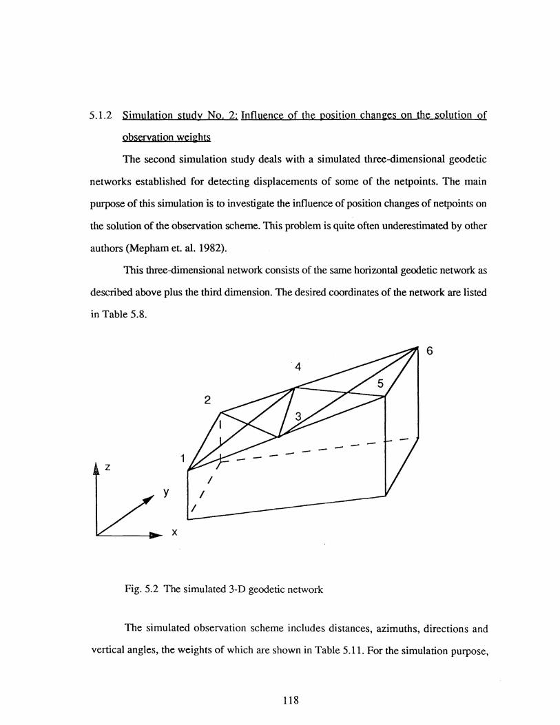
5.1.2 Simulation study No. 2: Influence of the position changes on the solution of
observation weights
The second simulation study deals with a simulated three-dimensional geodetic
networks established for detecting displacements of some of the netpoints. The main
purpose of this simulation is to investigate the influence of position changes of netpoints on
the solution of the observation scheme. This problem is quite often underestimated by other
authors (Mepham et al. 1982).
This three-dimensional network consists of the same horizontal geodetic network as
described above plus the third dimension. The desired coordinates of the network are listed
in Table 5.8.
6
1 z
y
X
Fig. 5.2 The simulated 3-D geodetic network
The simulated observation scheme includes distances, azimuths, directions and
vertical angles, the weights of which are shown in Table 5.11. For the simulation purpose,
118
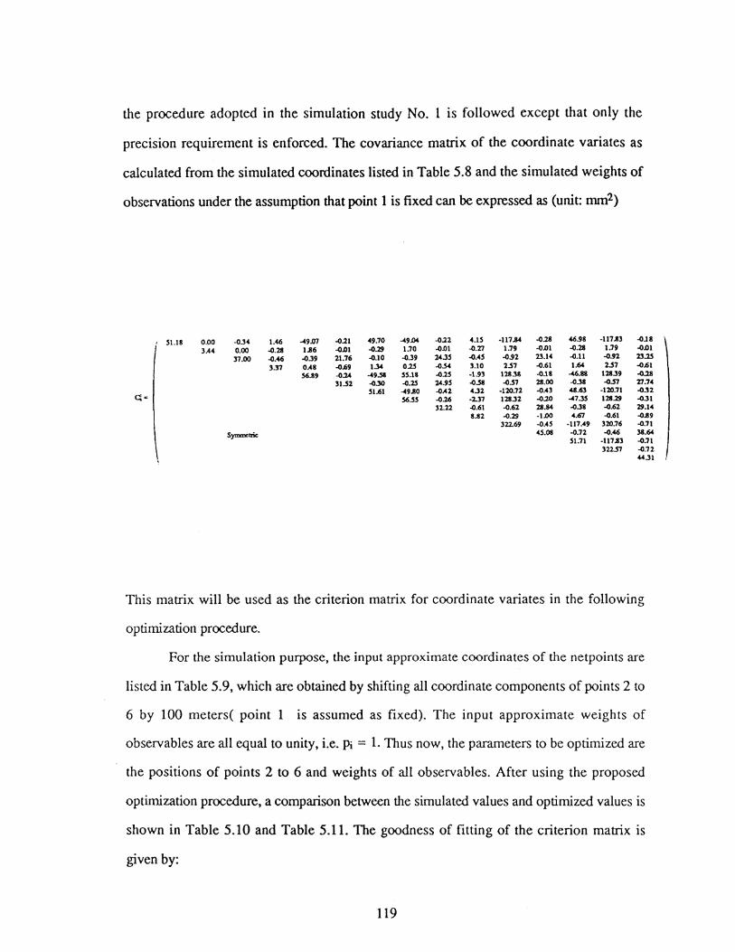
the procedure adopted in the simulation study No. 1 is followed except that only the
precision requirement is enforced. The covariance matrix of the coordinate variates as
calculated from the simulated coordinates listed in Table 5.8 and the simulated weights of
observations under the assumption that point 1 is fixed can be expressed as (unit: mm2)
' 51.18 0.00 -0.34 1.46 -49.177 -0.21 49.70 -49.04 -0.22 4.15 ·117.84 -0.28 46.98 -117..83 -OJ I
3.44 0.00 -0.28 1..86 -0.01 -0.29 1.70 -0.01 -0.11 1.79 -0.01 -0.28 1.79 -0.01
37.00 -0.46 -0.39 21.76 -0.10 -0.39 14.35 -0.45 -0.91 13.14 -0.11 -0.91 13.25
3.37 0.48 -0.69 1.34 0.25 -0..54 3.10 2..57 -0.61 1.64 1..57 -0.61
56.89 -0.24 -49..58 5s.t8 -0.25 -1.93 128.38 -OJ8 -46.88 128.39 -0.28
31.52 -0.30 -0.15 14.95 -0..58 -0..57 28.00 -0.38 -0..57 17.74 51.61 -49..80 -0.42 4.32 -120.72 -0.43 4U3 -120.71 -0.32
q~ S6.SS -0.26 -2.37 128.32 -0.20 -47.35 128.29 -0.31 32.22 -0.61 -0.62 28.84 -0.38 -0.62 29.14
8.82 -0.29 -1.00 .4.67 -0.61 -0..89 322.69 -0.45 -117.49 320.76 -0.71
S:ymmctric 45.08 -0.72 -0.46 38.64 51.71 -117..83 -0.71
322.57 -0.72 44.31
This matrix will be used as the criterion matrix for coordinate variates in the following
optimization procedure.
For the simulation purpose, the input approximate coordinates of the netpoints are
listed in Table 5.9, which are obtained by shifting all coordinate components of points 2 to
6 by 100 meters( point 1 is assumed as fixed). The input approximate weights of
observables are all equal to unity, i.e. Pi = 1. Thus now, the parameters to be optimized are
the positions of points 2 to 6 and weights of all observables. After using the proposed
optimization procedure, a comparison between the simulated values and optimized values is
shown in Table 5.10 and Table 5.11. The goodness of fitting of the criterion matrix is
given by:
119

-4.94 0.30 0.11 0.$1 6.25 0.11 ·S.l6 6.14 ..O.ll 0.43 1].07 0.26 -4.$5 ll.47 ..0.04 ..O.Ol .0.01 .0.30 .0.05 0.22 ..0.26 -o.os .0.07 ..Q.67 ..0.07 0.11 ..0.64
0.07 0.04 ..O.Il 0.31 0.19 ..O.ll 0.11 0.01 -o.JS 0.11 0.2A ..0.$4 .0.01 -o.,. 0.01 0.$1 ..0.$6 0.14 0.00 ·1.31 ..0.01 0.$1 ·1.34
-1.11 ..0.20 6.71 -7.$3 0.20 .0.45 -ltl.ll ..O.ll 5.76 -15.74 0.40 0.30 ..0.17 O.lS 0.01 .0.11 0.00 0.34 ..0.94
-5.61 6.19 ..0.14 0.31 1].$0 0.30 -4.76 ll.89
c.-q· -7.11 0.19 .0.39 ·U.M ..0.29 5.$1 -15.17 0.31 0.01 0.11 0.00 ..O.Ol 0.01
0.11 ·1.15 ..O.Q6 0.60 -1.11 ·]l.40 ..0.&7 11.19 -30.ll
Syuano>trio: ..0.4] 0.46 -1.41 .].69 10.17
-11.41
From the above results we can see that the fitting of the criterion matrix is perfect, i.e. the
covariance matrix of the optimized network is in fact the same as that of the simulated
network. From Table 5.11, all the optimized weights of observables are practically the
same as the simulated weights. Table 5.10 shows, however, that except in the z-direction,
some of the position shifts in x- andy-direction are not correctly back shifted. It means that
the precision of the network is mostly affected by changes in positions in the z-direction
while position changes of certain values in some of the positive x- and/or y-direction of
some points do not contribute to the improvement of the precision. This finding obviously
reflects the importance of optimization of the geometric configuration of a network.
However, some authors may advocate that small changes in relative positions of stations
have no significant effect on the accuracy and thus there is no need for the optimization of
the configuration. This point of view is not pertinent. For instance, if in this example we
neglect all the simulated position shifts in x-, y-, and z-directions and if we would apply the
Second Order Design instead of the simultaneous First Order and Second Order Designs,
then a comparison between the simulated weights and the optimized weights is shown in
120
..0.1]
..O.D6 O.l6 ..0.01 0.09 0.07 ..O.G9 0.10 . IQ-13 0.04 ..0.04 0.15 ..0.46 ..0.()4 ..0.11 -o.n

Table 5.12. The results show that by neglecting changes of positions we would obtain an
observation scheme which would be much different from the simulated observation
scheme, and the fitting of the criterion matrix would be very bad, as reflected by the
following matrix (the variance-covariance matrix of coordinates minus the criterion matrix):
i 12.30 -2.93 -0.15 3.25 -12.06 -0.91 12.01 ·12.02 -0.73 3.90 -:1.4.30 -0.83 11.36 ·24.30 0.23 -1.7l -0.22 2.92 ·l.o7 -2.88 2.91 ·1.14 -0.38 6.69 ·IJO -2.72 6.69
6.77 -1.12 -1.32 6.55 -0.61 -1.25 U2 -1.04 -1.15 5.39 -0.68 -1.85 0.7:1 -3.50 -1.57 3.25 ·3.44 -1.19 0.42 -7.77 ·1.39 3.09 -7.77
11.46 ·1.116 -11.n 11.45 -1.10 -4.14 22.85 -1D7 ·1l.CJ7 22.86 6.79 -0.81 -0.99 4.37 ·1.46 ·1.85 5.83 -0.93 -1.85
U.73 -11.68 -0.65 3.19 -n.s5 -0.74 11.119 -23.55 C.•qE 11.44 ·1.07 -4.08 22.86 -1.02 -11.04 22.87
2.24 -1.11 -1.71 3.04 -0.71 -1.71 0.65 -9.02 -1.31 3.68 -9.03
44.93 -1.74 -22.29 44.94 Symmclric 5.03 -0.85 -1.74
10.52 -22.29 44.96
Here we can see that the maximum difference between the elements of the criterion
matrix and that of the covariance matrix calculated from the optimization results reaches to
44.96 rnm2. Therefore, this example shows that the influence of even 4% changes in
relative positions of stations on the improvement of network precision can be very
significant. Generally, different configurations may give quite different optimal solutions
for weights of observations. In this example, the constraints of Eq.(4-30) are not applied.
A good fitting of the criterion matrix of coordinate variates can be achieved only by
significantly increasing the weights of observations if changes of the configuration are
neglected. This point of view will be further elaborated in the following optimization
example.
121
-0.80 -1.11 5.31 -1.37 -1.119 5.13 -0.71 -1.05 2.96 -1.28 -1.78 4.76 -0 . .82 -1.78 4.52

Table 5.8:
Point
1
2
3
4
5
6
Desired coordinates for the three-D. geodetic network
x (m) Y (m) z(m)
500.00 600.00 550.00
500.00 2600.00 650.00
2500.00 600.00 700.00
2500.00 2600.00 700.00
5500.00 600.00 800.00
5500.00 2600.00 800.00
Table 5.9: The input approximate coordinates for the three-D. geodetic network
Point x (m) v (m) z(m)
1 500.00 600.00 550.00
2 600.00 2700.00 750.00
3 2600.00 700.00 800.00
4 2600.00 2700.00 800.00
5 5600.00 700.00 900.00
6 5600.00 2700.00 900.00
122
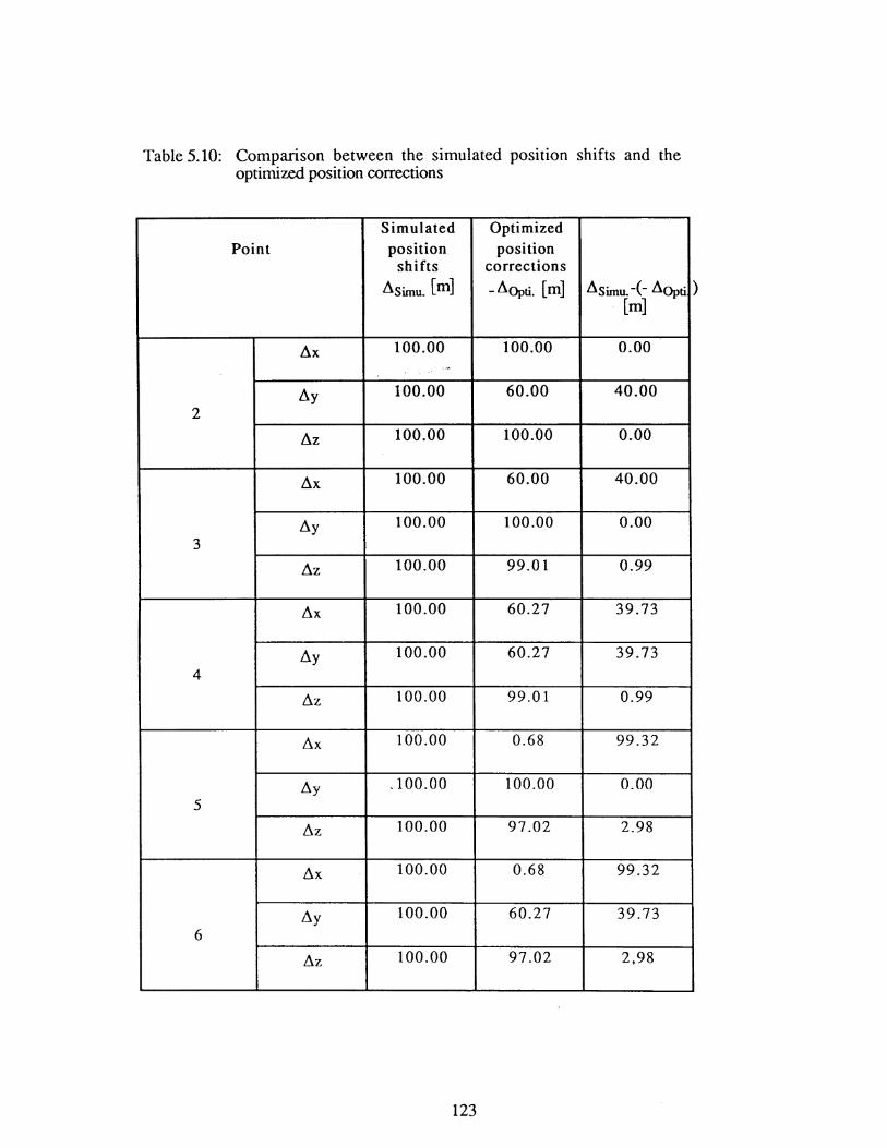
Table 5.10: Comparison between the simulated position shifts and the optimized position corrections
Simulated Optimized Point position position
shifts corrections
.1simu. [m] -.10pti. [m] .1simu. -(- .1apu . [m]
.1x 100.00 100.00 0.00 ,,.
.1y 100.00 60.00 40.00
2
.1z 100.00 100.00 0.00
.1x 100.00 60.00 40.00
.1y 100.00 100.00 0.00 3
.1z 100.00 99.01 0.99
.1x 100.00 60.27 39.73
.1y 100.00 60.27 39.73 4
.1z 100.00 99.01 0.99
.1x 100.00 0.68 99.32
.1y .100.00 100.00 0.00 5
.1z 100.00 97.02 2.98
.1x 100.00 0.68 99.32
.1y 100.00 60.27 39.73 6
.1z 100.00 97.02 2,98
123
)

Table 5.11 :· Comparison between the simulated weights and the optimized weights
Simulated Optimized Observables weights weights (psimu. - POpti.
( PSimu.) ( POpti. )
1 - 2 0.24768 0.24768 0.00000 1 - 3 0.24768 0.24768 0.00000 1 - 4 0.12409 0.12409 0.00000 2 - 3 0.12409 0.12409 0.00000
distances 2- 4 0.24768 0.24768 0.00000 3 - 4 0.24768 0.24768 0.00000 3 - 5 0.11058 0.11058 0.00000 3 - 6 0.07672 0.07672 0.00000 4- 5 0.07672 0.07672 0.00000 4- 6 0.11058 0.11058 0.00000 5 - 6 0.24768 0.24768 0.00000 1 - 2 1.00000 1.04012 0.04012
azimuth 5 - 6 1.00000 1.04012 0.04012
1 - 2 1.00000 1.04012 -0.04012 1 - 3 1.50000 1.56019 -0.06019 1 - 4 2.00000 2.08025 -0.08025 2 - 3 2.50000 2.60031 -0.10031 2- 4 3.00000 3.12037 -0.12037
vertical 3 - 4 3.5000.0 3.64043 -0.14043 angles 3 - 5 4.00000 4.1605 -0.1605
3 - 6 4.50000 4.68056 -0.18056 4- 5 5.00000 5.20062 -0.20062 4- 6 5.50000 5. 72068 -0.22068 5 - 6 6.00000 6.2407 5 -0.24075
station 1 1.00000 1.04012 -0.04012 station 2 1.50000 1.56019 -0.06019 station 3 2.00000 2.08025 -0.08025
directions station 4 2.50000 2.60031 -0.10031 station 5 3.00000 3.12037 -0.12037 station 6 3.50000 3.64043 -0.14043
124

Table 5.12: Comparison between the simulated weights and the optimized weights (SOD only)
Simulated Optimized Observables weights weights (Psimu. - Popti.
( PSimu.) ( POpti. )
1 - 2 0.24768 0.24073 0.00695 1 - 3 0.24768 0.25406 -0.00638 1 - 4 0.12409 0.13198 -0.00789 2- 3 0.12409 0.12392 0.00017
distances 2-4 0.24768 0.24628 0.00140 3- 4 0.24768 0.24903 -0.00135 3- 5 0.11058 0.10535 0.00523 3 - 6 0.07672 0.07455 0.00217 4-5 0.07672 0.07659 0.00013 4- 6 0.11058 0.10869 0.00189 5-6 0.24768 0.24866 -0.00098 1 - 2 1.00000 0.64888 0.35112
azimuth 5 - 6 1.00000 1.46813 -0.46813
1 - 2 1.00000 0.46274 0.53726 1 - 3 1.50000 0.02951 1.47049 1 - 4 2.00000 4.50279 -2.50279 2- 3 2.50000 3.61813 -1.11813 2- 4 3.00000 2.90386 0.09614
vertical 3- 4 3.50000 3.28663 0.21337 angles 3 - 5 4.00000 4.88663 -0.88663
3 - 6 4.50000 7.15309 -2.65309 4- 5 5.00000 2.61994 2.38006 4- 6 5.50000 5.08790 0.41210 5 - 6 6.00000 5.64983 0.35017
station 1 1.00000 0.69075 0.30925 station 2 1.50000 2.34522 -0.84522 station 3 2.00000 1.92279 0.07721
directions station 4 2.50000 2.18637 0.31363 station 5 3.00000 2.82130 0.17870 station 6 3.50000 3.55782 -0.05782
125

5.2 Optimization Examples
In the previous sections, the simulated study No. 1 show the validity of the
developed mathematical models. Study No. 2 illustrated the significance of applying
position changes of netpoints to the optimal solution of observation ~eights. The latter
point is further elaborated in the following optimization example No. 1, where the practical
significance of the newly developed methodology is illuminated by approaching a practical
design problem. Through a comparison of the results obtained by different methods, the
advantages of the new approach over the others are easily identified.
The application of the developed optimization algorithm goes to a practical geodetic
network established to assist in deformation monitoring and analysis of the structures of a
hydro-power generation station in Mactaquac, N.B., Canada.
5.2.1 Example No. 1: Optimal design of a monitoring network- Comparison of different
approaches.
Suppose we are given a monitoring network to be optimally designed as shown by
Fig. 5.3. The approximate coordinates of the netpoints are listed in Table 5.13. The
minimum and maximum side lengths of the network are approximately 1.7 km and 5.9 km,
respectively. Assume that the deformation model to be detected includes a homogeneous
strain field over the whole area plus single point movements of points 3, 4 and 5. That is,
the vector of deformation parameters to be detected can be expressed as:
~ = (dx3 dy3 dX4 dy4 dxs dys Ex Exy Ey)T
where dxi, dyi (i=3, 4, 5) represent the displacements of points 3, 4 and 5 in x- and y
directions respectively, and Ex, Ey and Exy the normal strain and shear strain parameters
respectively. The deformation model can be expressed as:
126

3
X
Fig. 5.3: The monitoring network
Table 5.13: The approximate coordinates of the monitoring network
Point x(m) y(m)
1 1125.00 1625.00
2 4625.00 375.00
3 6250.00 4625.00
4 3250.00 5875.00
5 3375.00 1500.00
6 4375.00 4625.00
127

Ui = Ex Xi + Exy Yi
Vi = Exy Xi + Ey Yi
Uj =dxj + Ex Xj + Exy Yj
Vj =dyj + Exy Xj + Ey Yj
for i=l, 2, 6; and
for j=3, 4, 5.
To simplify the computation, only the precision criterion is considered here. A diagonal
matrix:
~ = 2· Diag{(0.5 mm)2 · · · (0.5 mm)2 (O.lppm)2 ••• (0.1ppm)2 }
is adopted as the criterion matrix of the deformation parameters for the optimization. That
is, the standard deviations to be achieved for the detection of the displacements are
respectively 0.71 mm, and those for strain parameters are 0.14 ppm.
To achieve the above set precision criteria, the optimal configuration of the network
and optimal weights of observations have to be solved for. Assume that all the distances
will be measured with EDM instruments with achievable accuracies ranging from
cr1 = (lmm)2 + (1 ppm s)2 to cr1 = (0.1 ppm s)2 , and assume that the positions of points 1
and 2 cannot be changed, while the possible changes of positions for points 3, 4, 5 and 6
range from -200 m to +200 m in both x- and y-directions respectively. The input
approximate weights for distances are calculated from the initial accuracy of instruments
i.e. cr1 = (lmm)2 + (1 ppm s)2 and are listed in Table 5.15. Therefore, the unknown
parameters to be optimally solved for include the position changes to be introduced to
points 3, 4, 5, and 6, and changes to the weights of all the distances.
To approach the above optimal design problem, the following different possible
methods may be applied:
Method I-- Analytical Second Order Design CSQD) only;
128

Method II-- The conventional approach: To perform the First Order Design
(FOD) by trial and error first, and then apply the analytical Second
Order Design;
Method III-- The modified conventional approach: To perform analytical First
Order Design first~ and then do analytical Second Order Design;
Method N -- The newly developed approach: To perform the simultaneous First
Order and Second Order Design analytically.
At first, Method I is used since one used to underestimate the significance of
relatively small position changes of netpoints for the optimal design problem. Therefore,
for most of the real world design problems of engineering or monitoring networks, only
SOD is carried out. Method II is hard to follow. Since no fully analytical FOD algorithm
exists, one used to optimize the configuration of a network by trial and error, and,
therefore, to some extent subjective. The decision about how to change the configuration is
made through one's intuitive evaluation of the geometry of the network or by comparison
of the resulting variance-covariances matrix of the unknown parameters interactively with a
computer. Nevertheless, the exact numerical values of the position changes to be
introduced for the netpoints are very difficult to decide. The above difficulties may be the
main reason why the FOD did not deserve proper attention before. Although Koch ( 1982)
tried to develop an analytical algorithm for FOD, the derivatives needed in his mathematical
modelling are also provided by numerical method. In this case, the obtained derivatives will
be influenced by the selection of the step lengths needed. Therefore, instead of the
conventional approach, the modified conventional approach i.e., Method III is applied for
this example. Here, the developed fully analytical modelling in this research is used for the
FOD with the weights of observations fixed as the input approximate values, then the
desired weights of observations are solved for by fixing the resulting configuration of the
network. Finally, Method IY is the simultaneous FOD and SOD as developed in this
129

research. Here the all the unknown position changes of netpoints and obseiVation weights
are optimally solved simultaneously.
The results of applying Method I, Method III, and Method IY to the same design
problem are listed in Tables 5.14 to 5.16.
Table 5.14 shows that all the three methods have satisfied the set precision criteria.
However, from Table 5.15, we can see that to achieve the same objective, Method IV
requires the minimum weights. The total weight required from Method I is 15% larger than
that from Method Ill, and is 25% larger than that from Method IV. By identifying weights
as an indicator of cost, the obseiVation scheme as obtained from Method IV requires the
minimum cost. This shows once again that introducing even relatively small position
changes of netpoints has significance for the optimal design of a network. They should not
be neglected. Table 5.16 shows the possible position shifts of netpoints and the actual
shifts from method III and method IV.
!here is a serious problem with the modified conventional approach i.e., the
separate analytical FOD and SOD. Since at the FOD stage the weights of obseiVations have
to be fixed, the solution for position changes depends on the initially adopted approximate
values of the weights. This leads to different solution for the desired weights of
observations at the SOD stage for different approximate values of the weights adopted at
the FOD stage. This problem is overcome when the simultaneous FOD and SOD is
performed. Whatever initial approximate weights are adopted, they do not influence the
obtained results. This is illustrated by the numerical example. Tables 5.17 to 5.19 show the
results obtained by the separate FOD and SOD approach, and the Simultaneous FOD and
SOD approach when the maximum achievable weights are used as the approximate
weights. From Table 5.17, Table 5.18, and Table 5.19, one can see that to achieve the
same objective, after changing the input approximate weights of obseiVations, method IV
gives practically the same results as those obtained before. However, the results from
130
method III are quite different from those obtained before. The total weight amounts to
99.35, which is nearly twice as much as that given by method IV. Obviously this method is
not recommendable.
From the above discussion and numerical example, the following conclusions are
easily drawn:
1) If both the configuration of a network and weights of observations are to be
optimized, it is not recommended to perform SOD alone. By introducing
position changes of netpoints, a stronger geometry of the network can be
established. That .will lead to saving of effort in the field observation
campaign,.i.e., saving of money. In this example, if only 200 metres position
changes are considered, which amount to a 5% of the relative positions of the
network (the average side length of the network is 3.8 km), then such relatively
small changes in configuration have reduced the total weight by 25% as
compared to the case when these position changes are not introduced (i.e. SOD
only). Furthermore, if we allow the maximum possible coordinate changes for
each point up to± 400 meters, i.e. around 10% of the relative positions of the
network, then one can see from Table 5.20 that the required total weight as
obtained by the approach of simultaneous FOD and SOD is 47.43, which is
only 68% of that obtained by SOD only.
2) Because of the awkward procedure of the trial and error method, the
conventional separate FOD and SOD approach should be avoided.
3) By applying the fully analytical separate FOD and SOD approach, it is found
that the results of this approach are dependent on the input approximate weights
of observations. Different input approximate weights adopted at the FOD stage
will lead to different position changes to be introduced for the netpoints.
Therefore, they lead to different desired weights solved at the SOD stage.
Theoretically, this approach should lead to stable results only by performing a
131

number of FOPs and SODs iteratively. However, this cumbersome procedure
can now be avoided by the newly developed simultaneous POD and SOD
approach, the results of which are independent of the selection of the input
approximate weights.
4) From the above discussion, one may conclude that the approach of
simultaneous FOD and SOD' is the optimal approach to the optimal design
problem. Although this approach is induced by the concept of "introducing
relatively s~l position changes", large changes can actually be accommodated
by increasing the number of iterations during the solution procedure.
132
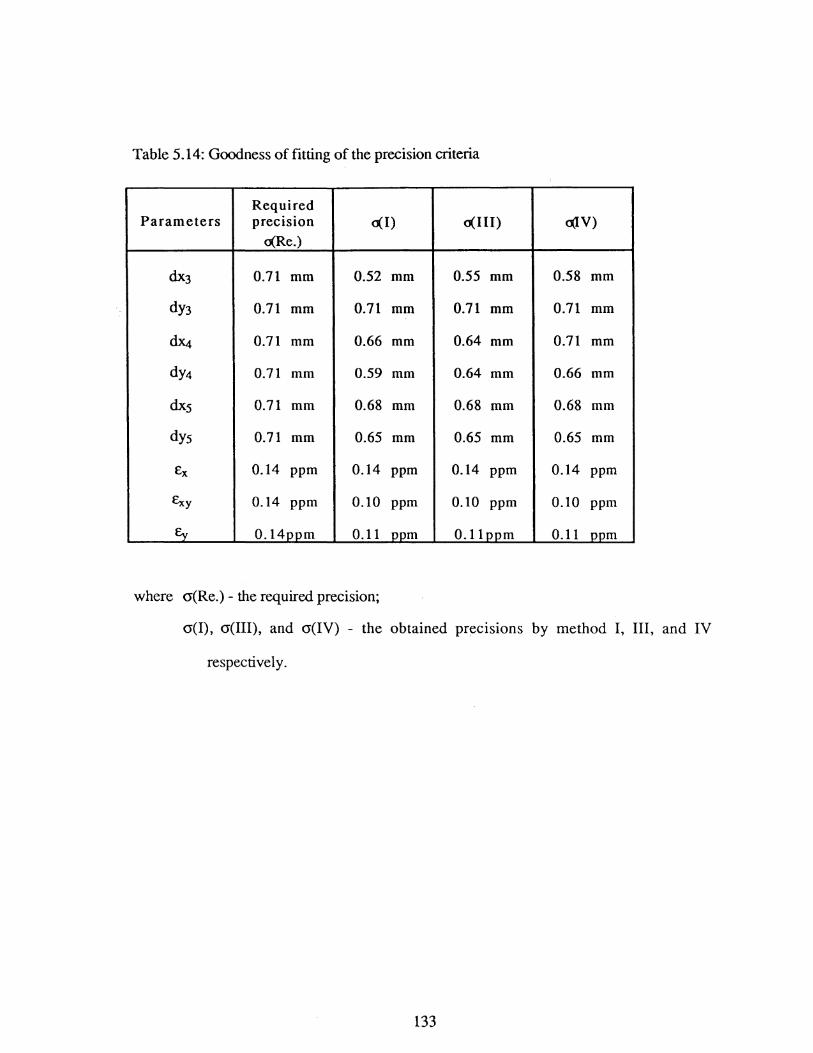
Table 5.14: Goodness of fitting of the precision criteria
Required Parameters precision o(I) o(III) aJV)
o(Re.)
dx3 0.71 mm 0.52 mm 0.55 mm 0.58 mm
dy3 0.71 mm 0.71 mm 0.71 mm 0.71 mm
dX4 0.71 mm 0.66 mm 0.64 mm 0.71 mm
dy4 0.71 mm 0.59 mm 0.64 mm 0.66 mm
dxs 0.71 mm 0.68 mm 0.68 mm 0.68 mm
dys 0.71 mm 0.65 mm 0.65 mm 0.65 mm
Ex 0.14 ppm 0.14 ppm 0.14 ppm 0.14 ppm
Exy 0.14 ppm 0.10 ppm 0.10 ppm 0.10 ppm
Ey 0.14ppm 0.11 ppm 0.11ppm 0.11 ppm
where o(Re.)- the required precision;
o(l), o(III), and o(IV) - the obtained precisions by method I, III, and IV
respectively.
133

Table 5.15: The desired weights of the observations obtained by different approaches
Distances o(Aoorox.) p(l) o(III) o(IV) p(Max.)
1 - 2 0.06751 5.01637 4.84161 4.80926 7.23982
1 - 3 0.02757 2.83562 2.83562 2.83562 2.83562
1 - 4 0.04241 4.42907 4.01781 4.35522 4.42907
1 - 5 0.16452 2.46406 2.20997 1.97162 19.69231
1 - 6 0.04863 5.11182 5.11182 5.11182 5.11182
2- 3 0.04608 4.83019 4.83019 4.83019 4.83019
2-4 0.03017 3.11133 3.11133 3.11133 3.11133
2- 5 0.26122 1.70221 1.84226 1.84898 35.35911
2- 6 0.05229 5.51724 5.51724 5.51724 5.51724
3- 4 0.08649 9.46745 7.46287 3.33546 9.46745
3- 5 0.05255 3.13335 3.02009 2.55709 5.54593
3 - 6 0.22145 7.63964 4.5133 4.11555 28.44444
4-5 0.04961 1.21321 1.02701 1.43396 5.22023
4- 6 0.26122 10.94819 6.96372 4.13256 35.35911
5 - 6 0.08499 2.50626 2.79949 2.93194 9.28882
Sum 1.49671 69.926 60.10433 52.89784 181.45249
where p(Approx.) - the input approximate weights;
p(Max) - the maximum achievable weights of observations;
p(I), p(III), and p(IV)- the solved weights by method I, III, and IV respectively.
134
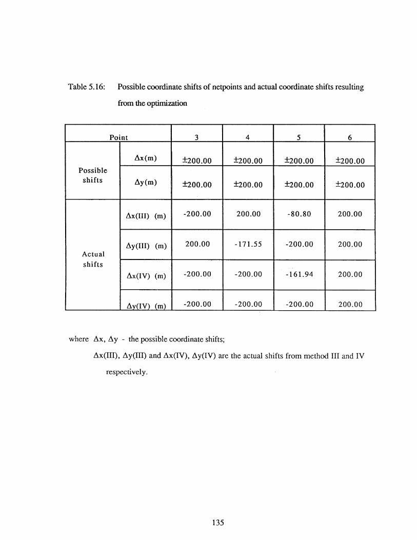
Table 5.16: Possible coordinate shifts of netpoints and actual coordinate shifts resulting
from the optimization
Point 3 4 5 6
Ax(m) ±200.00 ±200.00 ±200.00 ±200.00 Possible
shifts Ay(m) ±200.00 ±200.00 ±200.00 ±200.00
Ax(III) (m) -200.00 200.00 -80.80 200.00
Ay(III) (m) 200.00 -171.55 -200.00 200.00 Actual shifts
Ax(IV) (m) -200.00 -200.00 -161.94 200.00
i\y(IV) (m) -200.00 -200.00 -200.00 200.00
where Ax, Ay - the possible coordinate shifts;
Ax(III), Ay(III) and Ax(IV), Ay(IV) are the actual shifts from method III and IV
respectively.
135
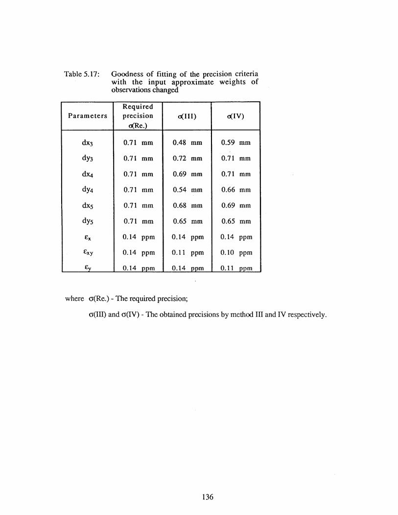
Table 5.17: Goodness of fitting of the precision criteria with the input approximate weights of observations changed
Required Parameters precision a( III) o(IV)
o(Re.)
dx3 0.71 mm 0.48 mm 0.59 mm
dy3 0.71 mm 0.72 mm 0.71 mm
dX4 0.71 mm 0.69 mm 0.71 mm
dy4 0.71 mm 0.54 mm 0.66 mm
dxs 0.71 mm 0.68 mm 0.69 mm
dys 0.71 mm 0.65 mm 0.65 mm
Ex 0.14 ppm 0.14 ppm 0.14 ppm
Exy 0.14 ppm 0.11 ppm 0.10 ppm
~ 0.14 ppm 0.14 ppm 0.11 ppm
where a(Re.)- The required precision;
a(III) and a(IV)- The obtained precisions by method III and IV respectively.
136

Table 5.18: The desired weights of observations with the input approximate weights of observations changed
Distances p(Approx.) p(lll) oliV) p(Max.)
1 - 2 7.23982 5.35699 4.80878 7.23982
1 - 3 2.83562 2.83562 2.83562 2.83562
1 - 4 4.42907 4.42907 4.33216 4.42907
1 - 5 19.69231 3.72786 1.92265 19.69231
1 - 6 5.11182 5.11182 5.11182 5.11182
2- 3 4.83019 4.83019 4.83019 4.83019
2- 4 3.11133 0.00000 3.11133 3.11133
2 - 5 35.35911 0.80252 1.88681 35.35911
2 - 6 5.51724 3.59146 5.51724 5.51724
3 - 4 9.46745 9.46745 3.37011 9.46745
3- 5 5.54593 2.61856 2.5296 5.54593
3 - 6 28.44444 17.07175 4.17594 28.44444
4 - 5 5.22023 1.54274 1.44492 5.22023
4 - 6 35.35911 35.35911 4.1002 35.35911
5 - 6 9.28882 2.6063 2.9281 9.28882
Sum 181.45249 99.35145 52.90548 181.45249
where p(Approx.) - the input approximate weights;
p(Max) - the maximum achievable weights of observations;
p(III), and p(IV)- the solved weights by method ill and IV respectively.
137

Table 5.19: Possible coordinate shifts and actual coordinate shifts with the input
approximate weights of observations changed
Point 3 4 5 6
Ax(m) ±200 ±200 ±200 ±200 Possible
shifts Ay(m) ±200 ±:200 ±:200 ±200
Ax(III) (m) 200.00 -200.00 200.00 -200.00
Ay(III) (m) 200.00 200.00 -200.00 -200.00 Actual shifts
Ax(IV) (m) -200.00 -200.00 -172.49 200.00
Ay(IV) (m) -200.00 -200.00 -200.00 200.00
where Ax, Ay - the possible coordinate shifts;
Ax(III), Ay(III) and Ax(IV), ~y(IV) are the actual shifts from method III and IV
respectively.
138

Table 5.20: Results of Method IV when the maximum possible position shifts can be up
to± 400 meters
The obtained precision Position shifts The optimized weights
Ax (IV)
Parameters o(IV) point Av (IV) distances
dx3 0.69 mm 1 - 2
-400.00 1 - 3
dy3 0.71 mm 3 1 - 4
-400.00 1 - 5
dX4 0.71 mm 1 - 6
4 -400.00 2- 3
dy4 0.69 mm 2- 4
-400.00 2- 5
dxs 0.69 mm 2- 6
5 -394.80 3 - 4
dys 0.71 mm 3 - 5
-400.00 3 - 6
Ex 0.13 ppm 4- 5
400.00 4 - 6
Exy 0.10 ppm 6 5 - 6
Ey 0.11 ppm 400.00 Sum
where o{IV)- the obtained precision by method IV;
Ax(IV), Ay(IV)- the actual position shifts from method IV; and
p(IV) - the obtained weights by method IV
139
p(IV)
7.23982
2.83562
3.41254
1.88894
5.11182
2.90403
3.11133
1.90803
5.51724
0.42232
1.25491
3.42277
1.45609
3.9237
3.01779
47.42695

5.2.2 Example No. 2: Optimization of the Mactaguac Monitoring Network
The Mactaquac generating station was constructed on the St.John River near
Fredericton, New Brunswick, between 1964 and 1968. It is comprised of a rock-fill dam,
a sluice-way, a 42 m high concrete gravity dam(intake and spillway), and a power house
with six power generating units connected to the intake structure via six penstocks of steel
plate encased in concrete. An illustration of the layout of the Mactaquac generating station is
shown in Fig. 5.4. A few years ago, some irregular deformations of the intake and power
house were noticed in addition to predicted seasonal expansions and contractions of the
structure. In order to find the source of the deformations a geodetic horizontal monitoring
network was established as part of the deformation monitoring scheme. It is a trilateration
network (Fig. 5.5) of 27 stations measured annually since 1983 using precision electronic
distance meters, i.e. Kern Mekometer ME3000 and Tellurometer MA200. Five object
points of the network, PR-1, PR-2, PR-3, TR-1, and TR-2, are located on the power
house, two, TK-1, and TK-7, on the top deck of the intake, and one point, M-1, is located
on the top of the spillway. The approximate coordinates of both the reference and object
points are listed in Table 5.21. The UNB Generalized Method was applied to determine
absolute displacements of the geodetic stations from various combinations of pairs of
survey campaigns. A report by Chrzanowski et al.(l988) has indicated systematic
downstream movement of points TR-1 and TR-2 at the average rate of 3 mrn/year, while
the roof points PR-1, PR-2, and PR-3 at a slower rate of about 2 mrn/year over the period
between 1985 and 1987. Most of the other stations exhibit significant, though random,
movements. This information has played an important role in the overall trend analysis of
the deformations.
In the 1989 campaign, an inverted pendulum, called INVP-B, near the object point
TR-1 on the power house was also included in the geodetic network. Thus the main
geodetic network now has 28 stations. The problem with the original observation scheme
140
is that accuracies of displacement detection for object points TR-1, TR-2, INVP-B and
some reference points such as C-200, C-555, etc. are not satisfactory to detect
displacements in the order of 2 - 3 mm/year. Also too many redundancies of distance
observations have been made. The author's approach has been applied to optimize the
observation scheme to enable the detection of movements of 2 mm/year of object points
with the available instrumentations and with the minimum effort. The configuration of the
monitoring network was not supposed to change.
Using the above developed optimization algorithm, and a diagonal matrix with all
diagonal elements being 0.36 mm2 (i.e., the standard deviations of all coordinates
components being 0.6 mm and the semimajor axises of the 95% point error ellipses being 2
mm) adopted as the criterion matrix, the following procedure was followed.
a) The datum of the monitoring network was selected as:
Fixed point C-400
Fixed Azimuth C-400--> 1-3
b) The optimization started with the original trilateration scheme (use EDM
ME3000, input accuracy oi = (0.3 mm)2 +( 2 ppm· s (mm))2) which consisted of
measuring 176 distances. These distances are shown in Fig. 5.5. The station 95% error
ellipses for this observation scheme are shown in Fig. 5.10.
c) Mter applying the optimization algorithm, 31 distances could be deleted because
they obtained zero values for their weights, i.e., they did not contribute to the improvement
of the network accuracy. The deleted distances are graphically shown in Fig. 5.6. The
station 95% error ellipses after deleting these distances. are shown in Fig. 5.11. From the
comparison between Table 5.22 and Table 5.23, one can see that deleting these 31
distances causes the semi-major axis of station 95% error ellipse of reference point C-200
to increase only by 0.3 mm, and the semi-major axes of station 95% error ellipses of all the
object points are effected by 0.1 mm at the maximum. This result shows that measuring the
141

31 distances could not add to the improvement of accuracies of displacement detection for
both the reference and object points. The optimized trilateration observation scheme is
shown in Fig. 5.7. The weights for all these distances are adopted as the ones achievable
using EDM ME3000.
d) From the original and optimized trilateration scheme the accuracies of points C-
100, C-200, C-555, REF-201, REF-202, TR-1, TR-2, INVP-B have not been
satisfactory, with the maximum semi-major axes of station 95% error ellipses being 6.1
mm and 5.4 mm for reference and object points, respectively. Thus roughly, in the worst
case, displacements less than 7.6 mm and 8.5 mm for object and reference points
respectively could not be detected. To improve the accuracies, the optimization algorithm
was applied again to optimize the monitoring network by adding to it direction
measurements.
Assuming the use of Kern E-2 electronic theodolite with minimum achievable
standard deviation of direction observation being 0.7", we have input all 28 possible
stations with total 352 directions as shown in Fig. 5.8. The optimization procedure has
shown that only 14 stations with a total of 88 directions would be good for the
improvement of the accuracies of the above mentioned points. The standard deviations of
direction observations given by the optimization algorithm for these stations are all 0.7".
These directions are graphically represented in Fig. 5.9. The station 95% error ellipses after
adding these directions are shown in Fig. 5.12. From Table 5.24, one can see that the
maximum semi-major axes corresponding to this optimized triangulateration observation
scheme are 2.9 mm and 2.2 mm (at 95%) for reference and object points, respectively.
Displacements larger than 4.1 mm and 3.1 mm for reference and object points respectively
would be detectable.
e) The optimization algorithm has also been used assuming that one's aim would be
to improve only the accuracies of object points TR-1, TR-2 and INVP-B. The optimization
procedure has indicated that only 5 stations with a total of 36 directions have to be
142

measured. These directions are graphically shown in Fig. 5.13. Table 5.25 shows that the
maximum semi-major axis of object points corresponding to this observation scheme is
also 2.2 mm (at 95% ). Thus Displacements larger than 3.1 mm are possible to be detected.
Fig. 5.14. shows a picture of station 95% error ellipses corresponding to this observation
scheme.
143

Table 5.21: The approximate coordinates of the Mactaquac monitoring network
Stations x(m) y(m)
C-400 864.511 576.27 1-3 1009.078 1180.25
REF-200 1152.051 1068.975 REF-100 738.534 1069.058
C-600 481.324 576.131 C-500 739.652 591.885 C-200 1584.227 1431.552 C-301 951.443 576.76 C-100 1143.233 558.283
REF-201 1273.949 1138.799 REF-202 1204.666 1200.884
C-555 958.596 1433.629 S-252A 360.764 813.886 S-251A 388.256 900.093 S-250A 432.046 979.683
DS-1 532.996 1078.807 DS-2 604.105 1138.284 1-1 887.909 1282.613 I-2 941.425 1231.489
PR-1 1043.291 986.334 PR-2 967.139 986.3 86 PR-3 903.871 986.275 M-1 816.993 1069.183 TK-7 914.345 1066.457 TK-1 1061.602 1066.493 TR-1 1055.058 981.482 TR-2 923.8 981.494
INVP-B 1031.826 982.221
144

Table 5.22: Station 95.000 % confidence ellipses for the original observation scheme (Factor used for obtaining these ellipses from standard error ellipses =2.4484)
Semi-major Semi-minor Azimuth of Stations axis axis Semi-major
axis (m) (m)
(o ' n)
1-3 0.0010 0.0001 13 27 39 REF-200 0.0015 0.0008 340 58 37 REF-100 0.0012 0.0008 1 27 40
C-600 0.0014 0.0009 335 46 17 C-500 0.0010 0.0008 354 30 19 C-200 0.0058 0.0016 326 59 42 C-301 0.0009 0.0008 1 46 58 C-100 0.0033 0.0011 69 36 12
REF-201 0.0031 0.0012 324 24 19 REF-202 0.0031 0.0014 294 47 55
C-555 0.0042 0.0013 303 25 29 S-252A 0.0016 0.0012 349 34 11 S-251A 0.0016 0.0011 351 5 57 S-250A 0.0016 0.0011 346 11 3
DS-1 0.0014 0.0010 354 5 16 DS-2 0.0013 0.0010 9 39 33 I- 1 0.0012 0.0010 56 47 6 I -2 0.0011 0.0008 33 9 49
PR-1 0.0011 0.0009 67 22 58 PR-2 0.0010 0.0010 284 20 9 PR-3 0.0011 0.0011 296 16 25 M-1 0.0012 0.0008 3 47 29 TK-7 0.0010 0.0008 10 18 2 TK-1 0.0009 0.0008 21 20 32 TR-1 0.0034 0.0013 290 57 28 TR-2 0.0030 0.0013 277 25 14
INVP-B 0.0053 0.0014 295 50 55
Total area of station ellipses= 0.19571D-03
145

Table 5.23: Station 95.000 % confidence ellipses after deleting 31 distances (Factor used for obtaining these ellipses from standard error ellipses =2.4484)
Semi-major Semi-minor Azimuth of Stations axis axis Semi-major
axis (m) (m)
(o ' n)
1-3 0.0011 0.0001 13 27 39 REF-200 0.0017 0.0009 340 47 19 REF-100 0.0012 0.0009 358 50 38
C-600 0.0016 0.0013 322 39 03 C-500 0.0011 0.0008 357 16 49 C-200 0.0061 0.0018 329 11 28 C-301 0.0010 0.0008 4 15 31 C-100 0.0035 0.0012 69 44 41
REF-201 0.0032 0.0012 324 21 18 REF-202 0.0032 0.0015 295 17 48
C-555 0.0043 0.0014 303 40 36 S-252A 0.0017 0.0012 349 13 35 S-251A 0.0016 0.0012 351 38 14 S-250A 0.0016 0.0011 347 31 52
DS-1 0.0015 0.0011 336 49 40 DS-2 0.0013 0.0011 10 12 46 1-1 0.0013 0.0011 52 9 20 I -2 0.0012 0.0008 24 7 52
PR-1 0.0012 0.0010 71 18 34 PR-2 0.0011 0.0010 283 30 14 PR-3 0.0012 0.0011 293 4 49
. M-1 0.0013 0.0010 16 8 13 TK-7 0.0011 0.0009 18 28 23 TK-1 0.0010 0.0009 19 33 34 TR-1 0.0035 0.0013 291 18 26 TR-2 0.0031 0.0013 277 37 57
INVP-B 0.0054 0.0014 295 49 51
Total area of station ellipses = 0.219650-03
146

Table 5.24: Station 95 % confidence ellipses for the optimized observation scheme (Factor used for obtaining these ellipses from standard error ellipses =2.4484)
Semi-major Semi-minor Azimuth of Stations axis axis Semi-major
aXIS (m) (m)
(o , ,)
1-3 0.0010 0.0001 13 27 39 REF-200 0.0010 0.0008 345 32 38 REF-100 0.0011 0.0008 357 19 27
C-600 0.0014 0.0012 319 23 54 C-500 0.0008 0.0007 318 50 48 C-200 0.0029 0.0015 328 49 19 C-301 0.0009 0.0007 7 19 19 C-100 0.0019 0.0010 67 7 16
REF-201 0.0014 0.0010 323 48 7 REF-202 0.0013 0.0010 309 33 27
C-555 0.0029 0.0013 301 18 57 S-252A 0.0015 0.0011 343 3 9 S-251A 0.0015 0.0011 345 45 44 S-250A 0.0015 0.0011 341 47 28
DS-1 0.0014 0.0011 329 0 52 DS-2 0.0012 0.0010 4 54 26 I- 1 0.0012 0.0011 70 19 51 I -2 0.0011 0.0008 26 40 34
PR-1 0.0011 0.0009 77 58 51 PR-2 0.0010 0.0009 287 54 56 PR-3 0.0011 0.0010 298 39 51 M-1 0.0012 0.0010 18 7 44 TK-7 0.0010 0.0008 17 33 53 TK-1 0.0009 0.0008 7 52 58 TR-1 0.0018 0.0012 292 59 42 TR-2 0.0017 0.0012 277 5 11
INVP-B 0.0022 0.0013 295 28 31
Total area of station ellipses= 0.12698D-03
147

Table 5.25: Station 95.000 % confidence ellipses for the optimized observation scheme (aim at improving accuracies of object points only, factor used for obtaining these ellipses from standard error ellipses =2.4484)
Semi-major Semi-minor Azimuth of Stations axis axis Semi-major
axis (m) (m)
( 0 I If)
1-3 0.0011 0.0001 13 27 39 REF-200 0.0016 0.0009 339 49 33 REF-100 0.0012 0.0009 356 43 54
C-600 0.0015 0.0012 318 22 33 C-500 0.0009 0.0008 316 7 47 C-200 0.0046 0.0017 329 17 51 C-301 0.0009 0.0008 5 51 18 C-100 0.0031 0.0011 70 58 37
REF-201 0.0023 0.0011 326 3 27 REF-202 0.0024 0.0014 295 4 9
C-555 0.0037 0.0013 303 1 42 S-252A 0.0016 0.0012 344 12 3 S-251A 0.0015 0.0011 347 6 30 S-250A 0.0015 0.0011 344 5 44
DS-1 0.0015 0.0011 331 1 26 DS-2 0.0012 0.0011 8 34 39 I- 1 0.0012 0.0011 63 58 11 I -2 0.0012 0.0008 25 3 56
PR-1 0.0012 0.0009 74 2 36 PR-2 0.0011 0.0009 281 35 45 PR-3 0.0012 0.0010 290 4 18 M-1 0.0012 0.0010 18 12 23 TK-7 0.0011 0.0009 21 46 7 TK-1 0.0010 0.0009 21 0 15 TR-1 0.0020 0.0013 292 10 38 TR-2 0.0018 0.0012 276 40 53
INVP-B 0.0022 0.0013 295 16 52
Total area of station ellipses= 0.164220-03
148

. :=.. ... : .::....:. .:--."
··-~'<
0 o:)O lOO
Fig. 5.4: Layout of the Mactaquac Generating Station
149
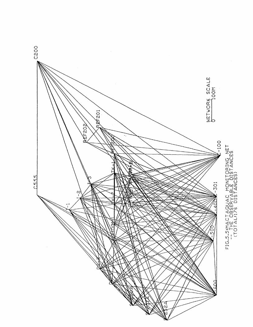
0 0 (\]
u
w _J
<l: U:L (})0
0
[

csss
os-2
s-250A
-100 ~ Jvv C-BOoJ::-30\
FIG.5.G:MAC1 AO\.JAC MONIIOR!NG NEI -- THE OELEIED DISTANCES BY
QPilMlZA TlON<IOI ALt3D
C200
ifJET'WOR-\ SCALE - OOM

~~~~------------------------------~C200
FIG.5.7:MACT AQUAC MONITORING NET -- THE OPTIMIZED TRILA TERA TION
~ETWOR~ SCALE lOOM

~C555 ~C200
F\G.S.B•MACT AGUAC MONITORING NET -- THE OBSERVABLE DIRECTIONS
TOTAL.: 352 DIRECTIONS
lfiET'WOR~ SCALE lOOM

r--............................. _______________ ~ C200
-100
F'IG.5 .9:MAC T AQUAC MONITORING NET --THE PROPOSED DIRECTIONS BY
OPTIMIZA TION<TOTAL:88)
~ETWOR\ SCALE OOM

~S-2
~S-1 c§l.EF'10~-1
c§-250A
c§-251A
j-252A
&-600 &-500
~555
d-1
J-2 .
J-3 \5EF'202
~EF'201
~00
JK-7 JK-1 <§EF'200
8cr~-~~1.B
C-400 ~-301
F'IG.5.10: 95% ERROR ELLIPSES THE ORIGINAL OBSERV. SCHEME
MACT AQUAC MONITORING NET
~TOR SCALE
~8~LE 0 MM (}-100
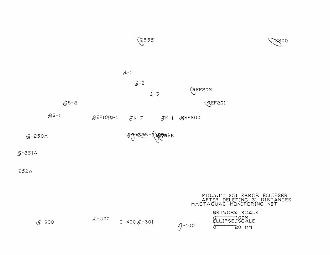
c9JS-2
c§IS-1 8EF'10~-1
c§-250A
:§-251A
252A
c§-600 &-500
~555
d-1
J-2
J-3 (5EF202
~EF'201
~00
cJK-7 JK-1 c§EF'200
8()W&f'-~Rl..B
C-400 &~301
F'IG.5.11: 95t ERROR EL.L.IPSES APTER DELETING 31 DISTANCES
MACT AQUAC MONITORING NET
· rTIIOR1 SCALE L.LIPSE &8~LE
0 MM (}-100

\5555 \S200
d-1
J-2
J-3 8EF202
£JS-2 8EF201
cQS-1 8-EFl0~-1 JK-7 JK-1 a,EF200
c§-250A ea-~-~l-s
c§-251A
~-252A
FIG.5.12: 95% ERROR ELLIPSES THE OPTIMIZED OBSERV. SCHEME
MACT AQUAC MONITORING NET
<§-600 &:-500
C-LWO ~-301 ~TOR SCALE
~8~LE 0 MM o:-100

DS-2
DS-1
S-250A
C555
I-1
I-2
-3
RE'.F10(}1-1
-100
F\G.s.l3•MACT AOUAC MONJTOF\JNG NET --THE PROPOSED DIRECTIONS BY
QPTIMlZA TlON<TOT AL:36)
lflET\.JOR~ SCALE -100M
C200

\5555 ~00
d-1
J-2
J-3 QJEF'202
£!S-2 ~EF'201
&S-1 8EF'l0~-1 cJK-7 (TK-1 c§EF'200
<§-250A ea--w£R-~~s
<§-251A
~-252A
F'IG.5.14: 95t ERROR ELLIPSES THE OPTIMIZED OBSERV. SCHEME
MACTAQUAC MONITORING NET
<§-600 &-500
C-L100 &-301 ~TOR SCALE
&8~LE 0 MM o-100


CHAPTER 6
SUMMARY OF RESULTS AND CONCLUSIONS
The objective of this study has been achieved. As a result of this research, some
conclusions and recommendations can be drawn.
The necessity of detecting, monitoring, and interpreting deformations is mainly
dictated by safety and scientific reasons. It is obvious that continuous and rigorous
monitoring of the natural or man-made environment is vital in predicting and preventing a
future disaster. The precise determination of variations of a body can support and aid in
improving new design theories by providing information about the load-deformation
relationship. The body knowledge on deformation mechanisms can also be enhanced,
which leads to the development of more sophisticated and refined procedures.
The aim of a monitoring scheme is to determine a set of deformation parameters
which characterize the changes of a deformable body in its dimensions, shape, and
position. Different methodologies and techniques, which may be classified as geodetic and
non-geodetic, can be used for this purpose. The selection of monitoring techniques
depends mainly on the type, magnitude, and rate of the expected deformation. Since each
method has advantages and disadvantages, the integration of different systems is highly
recommended to provide a more complete and more accurate picture of the deformable
body.
Before any deformation measurement campaign is started, the geodesists should
know about the result of their work according to the set objectives. This leads to the need
for the optimization and design of deformation monitoring schemes. Essentially, the
160

purpose for the optimization and design of monitoring schemes is to prevent the
deformation measurement campaigns from failing. It enables. us to make decisions on
which instruments should be selected from the hundreds of available models of various
geodetic and non-geodetic instruments and where they should be located in order to
estimate the unknown parameters and achieve the desired criteria derived from and
determined by the purpose of the monitoring scheme. It is for this reason that a
methodology for the optimization and design of deformation monitoring schemes has been
developed in this research.
In general, the unknown parameters to be optimized for a monitoring scheme
include the optimal positions for each geodetic and non-geodetic point characterized by
coordinates and optimal weights for each geodetic and non-geodetic observable. However,
from the practical point of view, since the specific positions of instruments in deformation
monitoring are rather suggested by landform in the monitoring area in connection with
mutual observability conditions and/or stability considerations, the unknown parameters to
be optimized for a monitoring scheme can be the "improvements" to the approximate
coordinates of both geodetic and non-geodetic points which are obtained by reconnaissance
in the field and the "improvements" to the approximate weights of the observations which
can be realized with the least effort. The optimal positions and weights are obtained then by
adding the solved "improvements" to their respective approximate values. The criteria of
optimization for monitoring schemes include precision, reliability, sensitivity, and
economy. The optimization of a monitoring scheme means to design a precise-, reliable-,
and sensitive enough scheme which can also be realized in an economical way. Precision is
a measure of the variance and covariance of the estimated parameters; reliability refers to the
measure to detect, localize and eliminate outlying observations; sensitivity refers to the
detection of minimum magnitude of parameters; and finally economy is a measure of cost
and benefit of the project. These criteria must be fulfilled for the different design problems
of a monitoring scheme. For the purpose of optimization, all the optimality criteria of
161

precision, reliability, sensitivity, and economy have to be expressed in terms of the
"improvements" to the approximate positions and weights. In addition, the "improvements"
to be. optimized are also subject to physical constraints constructed according to the
topography and/or stability conditions as well as the maximum achievable accuracies of
instruments. The proposed multi-objective optimization mathematical model can be applied
to solve for the optimal values of the "improvements" to be introduced.
As compared with the existing approaches for network optimization, the newly
developed methodology for the optimization and design of deformation monitoring
schemes has the following features:
(1) Any type of geodetic and non-geodetic observables can be considered to
construct an integrated deformation monitoring scheme. These may be the
coordinate observables from geodetic space techniques and photogrammetry,
individual terrestrial geodetic observations such as distances, directions,
azimuths, horizontal and vertical angles, levelling, etc, or any physical
mechanical measurements of tilts, strains, alignment observations, etc.
(2) The methodology can be used to design a monitoring scheme which will give
optimal results when solving for any type of deformation parameters. This is
reflected by the unspecified deformation model B ~. Following the concept of
the "UNB Generalized Approach" for deformation analysis, the whole
area covered by the deformation survey is treated as a non-continuous
deformable body consisting of separate continuous deformable blocks. Thus,
the blocks may undergo relative rigid body displacements and rotations, and
each block may change its shape and dimensions. In the case of single point
movement, the given point is treated as a separate block to be displaced as a
rigid body. Therefore, the methodology can be used to design a monitoring
scheme aiming at either displacement detection of unstable area or detection of
rigid body movements between blocks and the strain components. However, if
162

the deformation model B ~ to be detected consists of general polynomials, then
a monitoring scheme can be designed for the optimal solution of the unknown
coefficients in the polynomials. In the design phase, the a priori knowledge
about what deformation will take place may be used for the selection of an
appropriate deformation model. Such information will come from a study of
the relevant physical properties of the object; geomechanics for crustal
movement and structural analysis for deformation of dams, bridges and other
large structures, etc.
(3) Essentially, an QPtimization procedure tries to maximize or minimize some
kind of target function under a number of constraints( equalities or inequalities
or both). Formerly, it was very difficult, if not impossible, to construct such a
target function that contained parameters expressing precision, reliability,
sensitivity, and cost of observations all in the same utility unit. This difficulty
can now be overcome by introducing the theory of multi-objective
optimization. Rather than the "trial and error" method, all the criteria of
precision, reliability, sensitivity, and economy can now be expressed
analytically in terms of the unknown parameters to be optimized. Based on the
theory of multi-objective optimization, a suitable target function that includes
all the criteria can be formulated under a common scale and the multi-objective
optimization mathematical model (MOOM) for the optimization and design of
monitoring schemes is established. Thus it is now possible to consider all the
quality aspects i.e. precision, reliability, sensitivity and economy of a
monitoring scheme simultaneously.
(4) By identifying the unknown parameters to be optimized for a monitoring
scheme as the optimal positions for each geodetic and non-geodetic point
characterized by coordinates and optimal weights for each geodetic and non
geodetic observable, the developed methodology can analytically perform the
163

Combined First Order and Second Order Design (Vanicek and Kraki wsky,
1986) i.e. the simultaneous optimization of the geometrical configuration and
weights of heterogeneous observables in a monitoring scheme. For practical
applications, after appropriate optimality criteria for deformation parameters or
displacements are established, the optimization model MOOM gives us the
desired weights or standard deviations for each observable and it can also give
the desired position shifts of the initially selected netpoints in reconnaissance in
order to obtain the best configuration. From the given simulation studies and
practical examples one can see that even relatively small changes in
configuration may significantly contribute to the solution of an optimal design
problem. They can be used to establish a monitoring configuration with
stronger geometry, which may lead to significant savings of effort in the field
observation campaign. Conventionally, for positioning or monitoring
networks, one used to ignore small changes in relative positions of stations
assuming that they would have no significant contribution to the improvement
of the accuracy. This point of view has now been proved to be impertinent.
Although this methodology is induced by the concept of "introducing relatively
small position changes", relatively larger changes can actually be
accommodated by increasing the number of iterations during the solution
procedure.
If the positions of the netpoints selected in reconnaissance can not be
changed, the developed optimization model MOOM reduces to the Second
Order Design. On the other hand, if the measurement instrumentation and
accuracy for the given job are fixed, then the model reduces to the First Order
Design. Finally, if positions of some points and weights of some observables
have to be optimized, this model reduces to the Third Order Design. Therefore,
one can see that the conventional different Orders of Design Problem are
164

embeded in the proposed mathematical model. The author believes that the
optimization procedure developed in this research is the most practical and
flexible one for the optimal design of monitoring schemes or geodetic networks
established for engineering purposes. All the solutions are automatic thus
removing the need for the method of "trial and error".
(5) The developed methodology can be used for the optimal design of either one-,
two-, or three-dimensional monitoring schemes. The·developed mathematical
models can also be easily modifed to treat the optimization problems with the
Mixed Models, and the application of the methodology to the optimal design of
any geodetic networks for engineering purposes is quite straight forward
The examples with simulated and real data have shown that the developed
methodology is correct and works well. Further research is suggested to continue and
expand the practical applications of the developed methodology.
165

REFERENCES
Abbreviations
A VN :Algemeine Vennessungs-Nachrichten
Bull. Geod. :Bulletin Geodesique
CIS
DGK
JASA
'ZFV
: The Canadian Institute of Swveying
: Deutsche Geodatische Kommission
: Journal of American Statistics Association
: Zeitschrift fur Vermessungswesen
ALBERTA, J.E. (1974). "Planning and optimization of networks: Some general considerations." Boll. Geo<l. Sci. Aff. No. 33, pp. 209-240.
ALBERTA, J.E. (1980). A review of analysis techniques for engineering survey control schemes. Paper presented at the Industrial and Engineering Survey Conferences, London, UK.
BAARDA, W. (1962). "A generalization of the concept Strength of Figure." Publ. of the Computing Center of the Geodetic Inst., Delft.
BAARDA, W. (1967). "Statistical concepts in geodesy." Neth. Geod. Com .. publ. on Geodesy. New Series 2, No.4, Delft, Netherlands.
BAARDA, W. (1968). "A testing procedure for use in geodetic networks." Neth. Geod. Com .. publ. on Geodesy, New Series 2, No.5, Delft, Netherlands.
BAARDA, W. (1973). "S- Transformations and Criterion matrices." Neth. Geod. Com .. publ. on Geodesy, New Series 5, No. 1, Delft, Netherlands.
BAARDA, W. (1976). Reliability and precision of networks. VII International Course for Engineering Surveys of High Precision, Darmstadt, pp. 17-27.
BARAN, W. (1982). Some new procedures of sequential adjustment. Int. symp. on geodetic networks and computations ( 1981 ), DGK, Munchen, VIII: 69-79.
BOOT, J.C.G.(1964). "Quadratic Programming", North-Holland, Amsterdam, 1964.
BOEDECKER, G. (1977). The development of an observation scheme from the variance covariance matrix of the unknowns. Proc. Int. Symposium on optimization of design and computation of control networks. Sopron.
BOSSLER, J., E. GRAFAREND and R. KELM (1973). "Optimal design of geodetic nets 2." Journal of Geophysical Research, vol. 78, no. 26.
166

CHEN, Y.Q. (1983). Analysis of Deformation Surveys- A generalized method. Technical Report No. 94, Dept of Surveying Engineering, UNB, Canada.
CHEN, Y.Q., KA VOURAS M. and SECORD J.M. (1983). Design considerations in deformation monitoring. FIG XVII International Congress, Sofia, Bulgaria, Paper No. 608.2
CHEN, Y.Q., A. CHRZANOWSKI (1986). An overview of the physical interpretation of deformation measurements. at the Deformation Measurements Workshop, M.I.T., Cambridge, Mass. 31 October- I November 1986
CHRZANOWSKI, A. (1981). A comparison of different approaches into the analysis of deformation measurements. Proc. of FIG XVI International Congress, Montreux, Paper No. 602.3, August 9-18.
CHRZANOWSKI, A. (1983). Economization of vertical control surveys in hilly areas by using modified trigonometric levelling. Presented at the 1983 ACSM-ASP Convention, Washington, D.C., March.
CHRZANOWSKI, A., Y.Q. CHEN, J.M. SECORD (1983). "On the strain analysis of tectonic movements using fault crossing geodetic surveys." Tectonophysics, 97, pp. 295-315.
CHRZANOWSKI, A., and J.M. SECORD (1983). Report of the 'ad hoc' Committee on the Analysis of Deformation Surveys. Presented at the FIG-17th International Congress, Paper 605.2, Sofia, June 19-28.
CHRZANOWSKI, A. (1986). Geotechnical and other non-geodetic methods in deformation measurements. at the Deformation Measurements Workshop, M.LT., Cambridge, Mass. 31 October-1 November 1986
CHRZANOWSKI, A., Y.Q. CHEN, P. ROMERO, J.M. SECORD (1986). "Integration of geodetic and geotechnical deformation surveys in geoscience." Tectonophysics, 130, pp. 369-383.
CHRZANOWSKI, A., Y.Q. CHEN, J.M. SECORD, G.A. THOMPSON and Z. WROBLEWICZ ( 1988). Integration of geotechnical and geodetic observations in the geometrical analysis of deformations at the Mactaquac Generating Station. Conference 1988 on deformation surveys, Fredericton, Canada.
CONZETT, R., FRANK A. and MISSLIN C. (1980). Interactive triangulation. VIII Int. Kurs fur Ingenieurermessung, ZUrich.
COTTLE, R.W. AND G.B. DANTZIG (1968). "Complementary pivot theory of mathematical programming." Linear Algebra Application No. 1 (1968), 103-125.
CROSILLA, F. (1982). "Geodetic network optimization for the detection of crustal movements using a mekometer." Bollettino di Geo<lesia eSc. Affini.
CROSILLA, F. (1983a). "A criterion matrix for the second order design of control networks." Bull. Geod. 57:226-239.
167

CROSILLA, F. (1983b). "Procrustean transformation as a tool for the construction of a criterion matrix for control networks." Manuscripta Geodetica 8: 343-370.
CROSILLA, F. (1985). "A criterion matrix for deforming networks by multifactorial analysis" in Optimization and desi~n of ~eodetic networks edited by Grafarend and Sanso. Springer: Berlin etc. pp. 429-435.
CROSS, P.A. and B.M. WHITING (1980). The design of national vertical control networks. Proc. 2nd Int. Symposium On Problems Related to the Redefinition of Nonh American Vertical Geodetic Networks, Ottawa, Canada.
CROSS, P.A. and K. THAPA (1979). "The optimal design of levelling networks." Survey Review, vol. XXV, No.192, pp.68-79.
CROSS, P.A. and B.M. WHITING (198la). On the design of vertical geodetic control networks by iterative methods. VI International Symposium On Geodetic Computations, Munich.
CROSS, P.A. (1981b). The geodetic suite. Working paper 4, North East London Polytechnic, Department of Land Surveying, 92 pp.
CROSS, P. and A. FAGIR (1982). Procedures for the First and Second Order Design of vertical control networks. Proc. Survey Control Networks, Heft 7, Munch en.
CROSS, P.A. (1985). "Numerical methods in network design." in Optimization and design of geodetic networks edited by Grafarend and Sanso. Springer: Berlin etc. pp. 429-435.
DANTZIG, G.B.(1963). Linear programming and extensions. Princeton University Press, Princeton, N.J., 1963.
DERMANIS, A. (1985). "Optimization problems in geodetic networks with signals." in Optimization and design of geodetic networks edited by Grafarend and Sanso. Springer: Berlin etc. pp. 221-256.
DINKELBACH, W., H. ISERMANN (1973). "On decision making under multiple criteria and under incomplete information." in Multiple Criteria Decision Making, J.L. Cochrane and M. Zeleny, (eds.), Univ. of South Carolina Press, Columbia, South Carolina.
DUNNICLIFF, JOHN (1988). Geotechnical instrumentation for monitoring field performance. John Wiley & Sons, New York/ Chichester/ Brisbane/ Toronto/ Singapore/
DYER, J.S. (1972). "Interactive goal programming." Management Science, No. 19, pp. 62-70.
FAIG, W.(1978). The utilization of photogrammetry of deformations of structural parts in the shiping building industry. Proc. of the II international Symposium of deformation measurements by geodetic methods, Bonn, West Germany, Konrad Wittwer, stuttgart.
168

FAIG, W. and C. ARMENAKIS (1982). Subsidence monitoring by photogrammetry. Proceedines of the Fourth Canadian Symposium On Minine surveying and deformation measurements, Bannf, Alberta, June, CIS 197-208.
FRANK, C.F. (1966). "Deduction of earth strain from survey data." Bulletin Seismoloei<;al Society of America, 56 (1):35-42.
FRANK, A., MISSLIN C. (1980) INTRA: a programme for interative design and adjustment of geodetic networks. Institute flir Geodasie und Photogrammetrie, Eidgen6ssische Technische Hochschule ZUrich, Bericht 43, 11 pp.
GRAFAREND, E. (1972). "Genauigkeitsmasse geodatischer Netze." DGK-publ. A-73, Munch en
GRAFAREND, E.W. (1974). "Optimization of geodetic networks." Bolletino di Geodesia a Science Affini. Vol. 33, No.4, pp.351-406.
GRAFAREND, E.W. and B. SCHAFFRIN (1979). "Kriterion-matrizen 1-zweidimensional homogene und isotrope geodatische netze." ZFY, No.4, pp.133-149.
GRAFAREND, E.W., HEISTER. H., KELM R., KROPFF H. and SCHAFFRIN B. (1979). Optimierung geodetischer messoperationen. Karlsruhe
GRAFAREND, E.W. (1985). "Criterion matrices for deforming networks." in Optimization and design of geodetic networks edited by Grafarend and Sanso. Springer: Berlin etc. pp. 363-428.
GRAFAREND, E.W., F. KRUMM and B. SCHAFFRIN (1986). "Kriterion-matrizen III -zweidimensional homogene und isotrope geodatische netze." ZFV, No.5, pp.197-207.
HELMERT, F.R. (1868): "Studien tiber rationelle Vermessungen im Gebiet der hoheren Geodllsie." Z. Math. Phys. SchH:>milch vol. 13 (1868), pp. 73-120, 163-168.
HENDERSON, H.V, S.R. SEARLE (1979). "Vee and Vech operators for matrices with some uses in Jacobians and multivariate statistics." Canadian Journal of statistics 7,65-81
HUGGET, G.R. (1982). A Terrameter for deformation measurements. Proceedings of the Fourth Canadian Symposium on Mining Surveying and Deformation measurements, Banff, Alberta, June 7-9, CIS, 179.
ILLNER, M. (1986). "Anlage und Optimierung von Verdichtungsnetzen." DGK, C-317, Munich.
ILLNER, M. (1988). "Different models for the sequential optimization of geodetic networks." Manuscripta Geodaetica 13. (1988), 306-315.
JAGER, R. (1988). "Analyse und Optimierung geodatischer Netze nach spectralen Kriterien und mechanische Analogien." DGK, C-342, Munich, 1988.
169

JAGER, R. (1989). "Optimum positions for GPS-points and supporting fixed points in geodetic networks." Proc. lAG General Meeting (Edinburgh, 1989), Springer Lect. Notes, 1990.
JAGER, R., H. KALTENBACH (1990). "Spectral analysis and optimization of geodetic networks based on eigenvalues and eigenfunctions." Manuscripta Geo<laetica 15. ( 1990), 302-311.
JUNG, I. (1924). "Uber die gunstigste Gewischitsverteilung in Basisnetzen." Akadem. Ah.h. Uppsala 1924
KARADAIDIS, D. (1984). "A substitute matrix for photogrammetrically determined point fields." ITC-Joumal, 1984-3.
KARMAN, T. (1937). "On the statistical theory of turbulence." Proc. Natl. Acad. Sci. USA, 23.
KOCH, K.R. (1982a). "Optimization of the configuration of the geodetic networks." DGK, B, 258/III, 82-89, Munchen, 1982.
KOCH, K.R. ( 1985). "First Order Design: Optimization of the configuration of a network by introducing small position changes". in Optimization and design of geodetic networks edited by Grafarend and Sanso. Springer: Berlin etc. pp. 56-73.
KOCH, K.R. and D. FRITSCH (1981). "Multivariate hypothesis tests for detection of crustal movements." Tectonophysics, 71, pp. 301-313.
KUANG S.L. (1986). Study on the Post-Analysis of Positioning Data for Marine Geophysical Exploration. M.Sc.E thesis, Wuhan Technical University of Surveying and Mapping(WTUSM), April, 1986.
KUANG S.L. (1988). "Study of Outlier Detection and Position Estimation for Point Positioning in Marine Surveying." Journal ofWuhan Technical University of Surveying and Mapping(WfUSM), pp. 85-97, Vol. 12, No.4, 1988.
KUANG S.L. (1989) "Using Minimax Principle to Estimate Surveying Parameters and Perform Accuracy Analysis." Journal ofHohai University, pp. 16-23, Vol.17, No.3, 1989.
LIEW, C.K. and J.K. SHIM (1978). "Computer program for inequality constrained least squares estimation." Econometrica, vol. 46, pp 237.
MEISSL, P. (1976). "Strength analysis of two-dimensional Angular Anblock networks." Manuscripta Geodetica, Vol. 1, No.4.
MEPHAM, M.P.A., MACKENZIE A.P., KRAKIWSKY E.J. (1982). Design engineering and mining surveys using Interactive Computer Graphics. Presented at the 4th Canadian Symposium on Mining Surveying and Deformation Measurements, Banff, Canada.
170

MEPHAM, M.P.A., KRAKIWSKY E.J. (1983) Description of CANDSN: a computer aided survey network design and adjustment system. Presented at the 76th Annual meeting of the Canadian Institute of Surveying, Victoria, Canada.
MIERLO, J.VAN (1981). "Second Order Design: precision and reliability aspects." .A.YN. pp.95-101.
:MITfERMA YER, E. (1972). "Adjustment of free networks." ZFV, No. 11, pp. 481-489.
MOLENAAR, M. (1981). "A further inquiry into the theory of s-transformations and criterion matrices." Netherlands Geodetic commission. Publications on twodesy. New series, vol. 7, No. 1, Delft 1981
MULLER, H. (1986). Zur Berucksichtigung der Zuverlassigkeit bei der Gewichtsoptimierung geodatischerNetze." 'ZJ'V 111 (1986), 157-169
NICKERSON, B.G. (1979). Horizontal network design using computer graphics. M.sc. Eng. Thesis, Dept. of Surveying Engineering, UNB, Fredericton, Canada.
NIEMEIER, W. and G. ROHDE (1981). On the optimization oflevelling nets with respect to the determination of crust movements. lAG Symposium on Geodetic networks and computations, Munich.
NIEMEIER, W. (1982). Principal component analysis and geodetic networks-some basic considerations. Proc. of the meeting of FIG study Group 5B.
PEARSON, E.S., and H.O. HARTLEY (1951). "Charts of the power Function of the analysis of variance tests, derived from the non-central F-distribution." Biometrika, vol. 38, pp.112-130.
PELZER, H. (1971). Zur Analyse Geodatischer Deformationsmessungen, DGK, C 164, Munchen
RAMSAY, J.G. (1967). Folding and Fracturing of Rocks. McGraw-Hill, New York, 568 pp.
RAO, C.R. (1973). Linear statistical Inference and its applications. John Wiley & Sons, New York.
SAWARAGI, Y., H. NAKAYAMA AND T. TANINO (1985): Theory of multi-objective optimization. Academic Press, Inc. Orlando San Diego New York London Toronto Montreal Sydney Tokyo.
SCHAFFRIN, B. (1977). A study of the Second Order Design problem in geodetic networks. Proceedings of the International Symposium on Optimization of Design and Computation of control Networks, Sopron, 1977, pp. 175-177.
SCHAFFRIN, B., E.W. GRAFAREND, G. Schmitt (1977). "Kanonisches Design geodatischer Netze 1." Manuscripta Geodaetica 2 (1977) 263-306.
SCHAFFRIN, B., F. KRUMM and D. FRITSCH (1980). Positive diagonale genauigkeitsoptimierung von realnetzen uber den komplementaritatsalgorithms. VIII International Kurs Fur Ingenieurvermessung, Zurich
171

SCHAFFRIN 8.(1981). "Some proposals concerning the diagonal Second Order Design of geodetic networks." Manuscripta Geodetica, vol. 6, No.3, p.303-326
SCHAFFRIN, B. and GRAFAREND, E.W. (1982). "Kriterion-Matrizen 11-Zweidimensionale homogene und isotrope geodatische Netze." ZFV, Tei Ila, No. 5, pp. 183 - 194, Tei lib, No. 11, pp. 485 - 493, 1982.
SCHAFFRIN, B. (1983). "On some recent modifications regarding the optimal design of geodetic networks." Geo<iezja (Krakow) 1!l (1983), 43-56.
SCHAFFRIN, B. (1985a). "On design problems in geodesy using models with prior information." Statistics and Decision, Suppl. Issue 2 (1985), 443-453
SCHAFFRIN, B. (1985b). "Aspects of network design." in Optimization and design of geodetic networks edited by Grafarend and Sanso. Springer: Berlin etc. pp. 548-597.
SCHAFFRIN, B. (1986). "New estimation/prediction techniques for the determination of crustal deformations in the presence of geophysical prior information." Tectonophysics llQ (1986), 361-367.
SCHAFFRIN, B. (1988). Tests for random effects based on homogeneously linear predictors, in H. Lauter (ed.), Proc. of the Intl. Workshop on "Theory and Practice in Data Analysis", Acad. of Sci. of GDR, Report No. R-MATH-01/89, Berlin (East), pp. 209-227.
SCHMITT, G. (1977). Experience with the second order design of geodetic networks. Proc. International Symposium of Design and Computation of Control Networks, Sopron, Hungary.
SCHMITT G. (1978). Numerical problems concerning the second order design of geodetic networks. Second International Symposium Related to the Redefinition of North American Geodetic Networks, Washington.
SCHMITT G. (1980). "Second Order Design of free distance networks considering different types of criterion matrices." Bull. Geod. 54 pp. 531-543.
SCHMITT G. (1982). "Optimal design of geodetic networks." DGK, B, 258/III, 82-89, Munchen, 1982.
SCHMITI G. (1985). "A review of network designs, criteria, risk functions and design ordering." in Optimization and design of geodetic networks edited by Grafarend and Sanso. Springer: Berlin etc. pp. 6-10.
SCHMITI G. (1985). "Second Order Design". in Optimization and design of geodetic networks edited by Grafarend and Sanso. Springer: Berlin etc. pp. 74-121.
SCHMITT G. (1985). "Third Order Design". in Optimization and design of geodetic networks edited by Grafarend and Sanso. Springer: Berlin etc. pp. 122-131.
SCHONEMANN, P.H. (1966). "The generalized solution of the orthogonal procrustes problem." Psychometrica 31: 1-16.
172

SCHREIBER 0. (1882). "Anordnung der winkelbeobachtung im Gottinger Basisnetz." ZFY 11 (1882), 129-161
SECORD, J. M. (1985). Implementation of a generalized method for the analysis of deformation surveys. Technical Report No. 117, Dept. of Surveying Engineering, University of New Brunswick, Fredericton, N.B., Canada.
SECORD, J. M. (1986). Terrestrial survey methods for precision deformation measurements. at the Deformation Measurements Workshop, M.I.T., Cambridge, Mass. 31 October-1 November 1986
SOKOLNIKOFF, I.S. (1956). "Mathematical Theory of Elasticity." McGraw-Hill, New York.
SPRINSKY, W.H., (1978). "Improvement of parameter accuracy by choice and quality of observation." Bulletin Geodesique 52, 269-279.
TARLOR, G.I. (1935). "Statistical theory of turbulence." Proc. R. Soc. London, Ser. A, 151-421.
TANG, H.W.C. (1990). "Optimum design of geodetic network using integer linear programming and rank one updating procedure." M.Eng. thesis. Dept. of Surveying Engineering, Fredericton, UNB, Canada.
TESKEY, W.F. (1987). Integrated analysis of geodetic, geotechnical, and physical model data to describe the actual deformation behaviour of earthfill dams under static loading. Institute flir Anwendungen der geodllsie im Bauwesen. UniversiW.t Stuttgart, May, 1987.
TEUNISSEN, P.J.G. (1985)."Zero Order Design: Generalized inverses, Adjustment, the Datum problem and S-Transformations " in Optimization and design of geodetic networks edited by Grafarend and Sanso. Springer: Berlin etc. pp. 11-55.
TEUNISSEN, P.J.G. (1985)."Quality control in geodetic networks." in Optimization and design of geodetic networks edited by Grafarend and Sanso. Springer: Berlin etc. pp. 526-547.
VANICEK, P., E.J. KRAKIWSKY (1986). Geodesy: The Concepts. North-Holland publishing company.
VANICEK, P., A. KLEUSBERG, D. WELLS and R. LANGLEY (1986). "GPS survey design." in Guide to GPS positioning, Chapter 14. Canadian GPS associates. Printed in Fredericton, N.B.,.Canada by UNB Graphic Services.
WELLS, D.E., and E.J. KRAKIWSKY (1971). The method of least squares. Dept. of Surveying Engineering, University of New Brunswick, Fredericton, N.B., Canada.
WEMPNER, G.(1973). Mechanics of Solids with applications to thin bodies. McGrawHill, New York, 623 pp.
WHITTEN, A. (1982). Monitoring Crustal Movement, Lecture Notes used in P.R. China.
173

WHITTLE, P. (1954). "On stationary processes in the plane." Biometrika 41 (1954), pp. 434-449.
WIMMER, H. (1981). Second order design of geodetic networks by an iterative approximation of a given criterion matrix. VI International Symposium on geodetic computations, Munich.
WIMMER, H. (1982a). "Ein Beitrag Zur Gewichtsoptimierung geodatischer Netze." Pul. I2QK c -269, Munchen.
WIMMER, H. (1982b). "Second Order Design of geodetic networks by an iterative approximation of a given criterion matrix." DGK. Reihe B, Heft 258/III: 112-127.
WOLF, H. (1961). "Zur Kritik von Schreibers Satz uber die Gewichtsverteilung in Basisnetzen." ZEY 86 ( 1961 ), 177-179
174


APPENDIX I
NOMENCLATURE
1.1 General Conventions
1. Vectors are lowercase letters underscored, e.g., a.
2. Matrices are uppercase letters, e.g., A, or letters in parentheses, e.g., (a;.j); or
diag { a1, a2 · · ·} in the case of diagonal matrix with diagonal elements being
a1, a2 ···,or diag {A1, A2, ···}in the case of block diagonal matrix with A.j being
a submatrix.
3. Terminologies are consistent with
i) Wells and Krakiwsky (1971) for the least squares adjustment;
ii) Baarda (1968) and Rao (1973) for statistics;
iii) Chrzanowski (1981a) and Chen(1983) for deformation analysis;
iv) Grafarend (1974) for the optimization of networks.
1.2. Symbol Definition
E
I
e vee
is an element of
equal by definition
identity matrix
Khatri-Rao product
an operator obtained by stacking the columns of a quadratic matrix
one under another in a single column
175

1.3
1.4
vech an operator obtained by stacking the columns of a. quadratic matrix
one under another in a single column starting each column at its
diagonal element
Notations and Operations on Matrices A and B
AT transpose of A
IAI determinant of a sq~ matrix
A.l a matrix of maximum rank such that AT A .l =0
A- any generalized inverse of A (g-inverse) such that
AA-A=A
A+ pseudo-inverse or Moore-Penrose inverse such that
AA+A =A, A+AA+=A+, (AA+l =AA+, (A+A)T =A+A
r{A} rank of A
S(A) linear vector space generated by the columns of A
rd{A} rank defect of A
Tr(A} trace of A, equal to L ati
PNB projection operator onto S(A) along S(B)
Notations and Operations on vectors and Random Variables
11~11
<~.y_>
K,fl
E{~}
D{K}
V(~}
pr{~ > ~}
the norm of, or the length of~
inner product of~ and y_
~ is distributed as
expected value of~
dispersion matrix of~
variance of random variable ~
probability when ~ > ~
176

APPENDIX II
The Problems of OP. LP. JLCP
This appendix describes the problems of Quadratic programming(QP), Linear
Programming(LP), and the Linear Complementary Problem(LCP). For the details of the
solution methods, some references are suggested.
1) The Problem QP
Generally, the standardized form of the problem of Quadratic Programming can be
stated as:
Minimizel_ xT H x + cT x 2- - --
Subject to A~ ~ h
x~Q
Where x, ~ are n by 1 vectors;
H is a symmetric n by n matrix;
.b. is a m by 1 vector, and
A is a m by n matrix
(II -1)
(II-2a)
(II-2b)
When introducing a n+m by 1 vector Y = ( v'f, vi,···, v&-tn )T ~ Q of slack variables as
well as the vector of Lagrangian multipliers b.. the Lagrangian function can be set up as:
(II-3)
With I the n by n identity matrix. The minimum value of L1 ~. y_, b.) can be obtained by
setting the partial derivatives to zeros
177

dLt ( T ] -=Hx+~+ A -1 ~=Q dX (II-4)
dLl = [ A ] x + v { Q ] = 0 dA -I - - Q -
aL1 -= 2 Ai Vi for i=l, · · ·, m+n dVi (II-6)
Eq.(ll-6) may be reformulated as
AT y = .Q with A~ .Q and Y ~ !! (II-7)
Eq. (II-4)- Eq.(II-6) are the famous Kuhn-Tucker conditions for Quadratic programming,
which are necessary and efficient to get feasible solutions x for the problem QP. The
problem QP has a unique minimizing solution when H is positive definite and the
constraints (II-2) are feasible. Algorithm for the solution of a Quadratic Programming
problem can be obtained from Boot (1964). Alternatively, the above set of Kuhn-Tucker
conditions may be rewritten as
y=Ml!::+~
!} y = .Q with A~ .Q andy~ !!
k =(A H-I ~ + Q) H -I - £
)
(II-8a)
(II-8b)
This is called the Linear Complementarity Problem (LCP), which will be discussed later.
2) The Problem LP
The standardized form of the problem of Linear Programming is written as
Minimize Q. T X (II-9)
Subject to At X = .b.t (II-lOa)
178

~x:5:Jn
x~Q
Where .26 £ are the n by 1 vectors;
At. A2 are the m1 by n and lll2 by n matrices respectively; and
ht. h2 are the m1 by 1 and Illl. by 1 vectors respectively.
(II-lOb)
(II-10c)
The~e are different ways to approach the solution of a linear programming problem, in
which the Simplex Method due to G. Dantzig is firstly recommended. Details of the
approach refers to G. Dantzig(1963).
3) The Problem LCP
The problem of LCP is defmed as
Find y, f.. ~ Q.
Such that y=MA+k
yT_A=O
(II-lla)
(II-llb)
From Eq.(II-8), we can see that every Quadratic Programming can be transformed into an
equivalent LCP. In order to solve LCP, the Complementary Pivot Theory is applied.
Details of the method can be obtained from Cottle and Dantzig(l968), Lemke(l968). Liew
and Shim(1978) created a computer program suitable for the solution of this problem.
179

VITA
Candidate's full name: Kuang Shan-long
Place and date of birth: Jiangxi, P.R. China October 21, 1962
Permanent address:
Schools attended:
University attended:
Publications:
Department of Geology and Surveying Hohai University 1 Xikang Road, Nanjing P.R. China
J uxi Elementary School 1969- 1974
Wushu Middle School 1974- 1979
Wuhan Technical University of Surveying and Mapping 1979- 1983 B.Sc.E. 1983- 1986 M.Sc.E.
"Study on the Post-Analysis of Positioning Data for Marine Geophysical Exploration", M.Sc.E thesis, Wuhan Technical University of Surveying and Mapping(WTUSM), April, 1986.
"Study of Outlier Detection and Position Estimation for Point Positioning in Marine Surveying", Journal of Wuhan Technical University of Surveying and Mapping(WTUSM), pp. 85-97,
· Vol. 12, No.4, 1988.
"Using Minimax Principle to Estimate Surveying Parameters and Perform Accuracy Analysis", Journal of Hohai University, pp. 16-23, Vol.17, No.3, 1989.