deformation and fracture – lab course the bauschinger …

Lab Course on Deformation and Fracture – Bauschinger Effect 1

DEFORMATION AND FRACTURE – LAB COURSE

Autumn semester 2014

The Bauschinger Effect

Gabriella Tarantino

text by A. Rossoll (translated from French by D. Watson and A. Rossoll)

1. Definition of the Bauschinger effect The Bauschinger effect (BE) can be observed during tension–compression conditions and is associated with a decrease of the yield stress when the loading direction is reversed (Fig. 1). Such behaviour may have different origins: for instance, if due to residual macroscopic stresses, it is not a true Bauschinger effect. Macroscopic residual stresses may result from heat treatment or from cold work during manufacture. Two other causes exist. One of them, the principal cause, is related to the dislocation structure in the work-hardened metal. As deformation occurs, the dislocations accumulate at barriers (precipitates, grain boundaries) and form dislocation pile-ups and tangles. Two types of mechanisms are used to explain BE. First, local back stresses, which oppose the applied stress on the slip plane, are produced by dislocations pile-ups on slip planes at barriers (pile-up of dislocations at grain boundaries and Orowan loops around strong precipitates). Back stresses assist the movement of dislocations in the reverse direction due to their favourable orientation to the stress axis. Thus, the dislocations can move easily in the reverse direction and the yield strength of the metal is lowered. Secondly, when the slip direction is reversed, dislocations of opposite sign may be created at the same source that produced the slip-causing dislocations in the initial direction. Since dislocations of opposite sign attract and annihilate each other, the net effect is a further softening of the lattice. The other cause, known as “composite effect”, is due to zones of different yield strength inside the material, on a microscopic scale. This case is sometimes referred to as a pseudo-Bauschinger effect. The Masing or generalized Saint-Venant model describes this behaviour. Figure 2 shows a rheological model for two phases differing by their flow stress. Figure 3 shows the resulting behaviour.


Figure 1 Stress-strain curve demonstrating a Bauschinger effect. After load inversion, plastic deformation sets in at a lower stress (in absolute values) in compression than during the previous load cycle (stress at the reversal point).

Figure 2 Rheological model of the Masing or generalized Saint-Venant model, for two phases.


Figure 3 a Behaviour of individual phases of the model exposed in Fig. 2 (for E1 = E2), and b behaviour of the complete model. 2. Work hardening and hardening laws Plastic deformation of a material often induces work hardening (increase of flow stress). This is caused by the reduction of the dislocation mobility (dislocations interacting with each other and with barriers). Calculation of the plastic deformation of a structure then requires a description of the phenomenon with a suitable law. Two extreme cases may be distinguished: 2.1 Isotropic hardening The load surface undergoes a homothetic enlargement (dilation), Fig. 4a. Such hardening corresponds to the hindering of dislocation movement—whatever the direction—by increasing the number of barriers (formation of sessile dislocations). The von Mises yield criterion, well suited for plasticity of metals and polycrystalline alloys, is then written, very generally,

f J2(!) "! y (# pleq )( ) = 0, where

J2 designates the 2nd invariant of the deviatoric component of the stress tensor

! ;

! pleq is the equivalent accumulated plastic

deformation; and

! y (" pleq ) is the flow stress that increases with work hardening.

! y (" pleq ) is often

described by a power law, for example

! y = k + K(" pleq )n where k is the yield stress.


Figure 4 a Purely isotropic hardening; b purely kinematic hardening, for load surfaces projected in two dimensions. 2.2 Kinematic hardening (Bauschinger Effect) The load surface undergoes a translation in the direction of the load, Fig. 4b. The entire work hardening is thus covered by the load inversion, which leads to the Bauschinger effect. A general formulation for this, still for the von Mises criterion, is

f J2(!) " X( ) = 0. The tensor X represents translation of the load surface, where X = 0 is the neutral state. The simplest formulation, Prager’s linear kinetic work hardening law, Fig. 5, is written, for the von Mises criterion,

f = J2(! " X) " k = 32( # ! " # X ) : ( # ! " # X )$

% & '

1/ 2

" k (1)

The evolution of X is described as follows:

dX =23C ! d" pl where

! pl is the plastic deformation

tensor. A nonlinear formulation may often give a better description. It can be formulated by introducing a term that reflects an evanescent (fading) memory of the deformation path

dX =23C ! d" pl # $ !X ! d" pl

eq (2)

2.3 Mixed hardening Most materials present a combination of both types of hardening. However, in general one may often accurately describe low strain deformation with purely kinematic hardening laws, and large strain deformation with purely isotropic hardening laws. Note that other complications may arise


in real materials, like anisotropic plasticity already present before loading, or dependence of the plastic flow on the deformation rate, and so on.

Figure 5 Sketch of a linear and b non-linear kinematic hardening during a tension-compression load cycle. 3. Parameter identification for a kinematic work hardening law Parameter identification for a linear work hardening law is quite simple. It can be done from a simple tensile test. The plasticity criterion becomes

f = ! " X " k = 0 and the plastic flow

d!11pl = d! pl = d" (attention in the case of load inversion). The hardening modulus is then

constant and equals C, and

! = X ± k = C "# pl ± k . For non-linear work hardening, a flow potential different from the expression for the load surface f is chosen:

F = J2(! " X) +3 #$4 #C

X :X" k = f +3 #$4 #C

X :X (3)


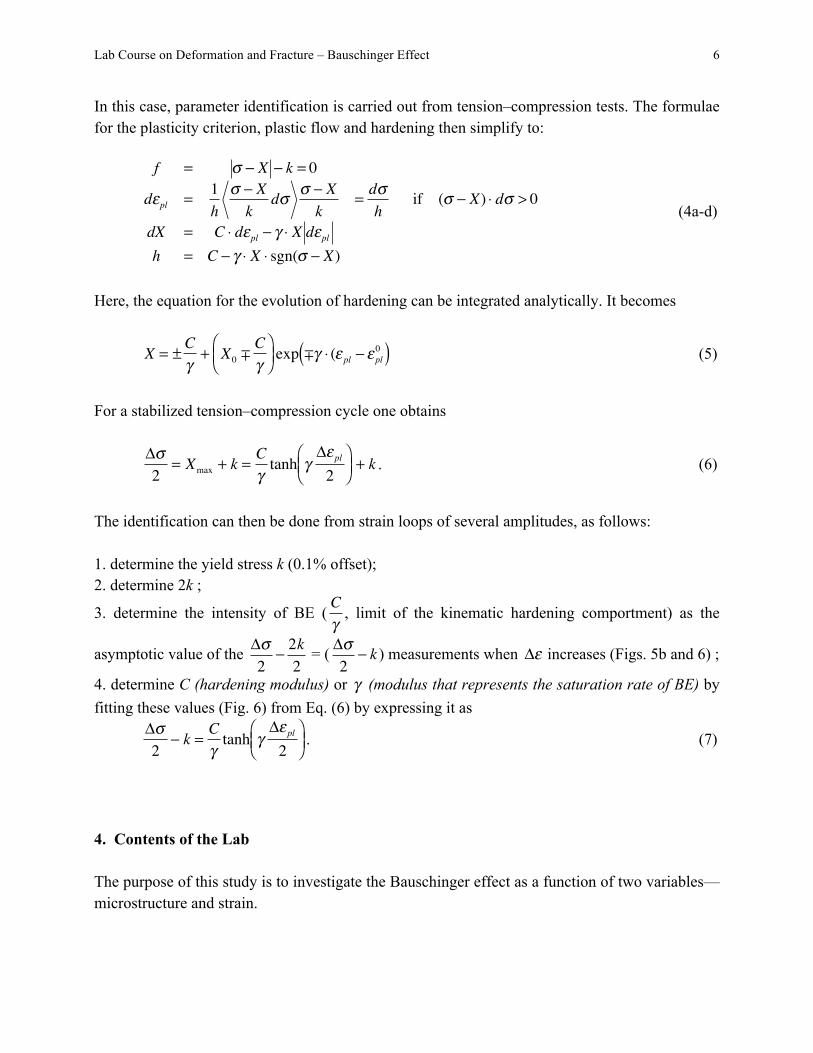
In this case, parameter identification is carried out from tension–compression tests. The formulae for the plasticity criterion, plastic flow and hardening then simplify to:

f = ! " X " k = 0

d#pl = 1h

! " Xk

d! ! " Xk

= d!h

if (! " X) $ d! > 0

dX = C $ d#pl " % $ X d#plh = C " % $ X $ sgn(! " X)

(4a-d)

Here, the equation for the evolution of hardening can be integrated analytically. It becomes

X = ±C!

+ X0 !C!

" # $

% & ' exp !! ( () pl * ) pl

0( ) (5)

For a stabilized tension–compression cycle one obtains

!"2

= Xmax + k =C#tanh #

!$ pl2

% & '

( ) * + k . (6)

The identification can then be done from strain loops of several amplitudes, as follows: 1. determine the yield stress k (0.1% offset); 2. determine 2k ;

3. determine the intensity of BE (

C!

, limit of the kinematic hardening comportment) as the

asymptotic value of the

!"2

# 2k2

= (

!"2

# k ) measurements when

!" increases (Figs. 5b and 6) ;

4. determine C (hardening modulus) or

! (modulus that represents the saturation rate of BE) by fitting these values (Fig. 6) from Eq. (6) by expressing it as

!"2

# k =C$tanh $

!% pl2

& ' (

) * + . (7)

4. Contents of the Lab The purpose of this study is to investigate the Bauschinger effect as a function of two variables—microstructure and strain.


Figure 6 Identification of coefficients C and

! , here from three tension–compression cycles of different strain amplitudes. 4.1 Materials and samples A classical aluminium alloy as frequently used in aerospace applications will be studied. Although it is normally commercialized as sheet metal, the samples have been machined from drawn bars of circular cross-section. The alloy is 2015 (4.2Cu-1Sn-0.9Mg-0.6Mn-0.3Bi), which is a lead-free alloy dedicated for free machining and will be tested with the following heat treatments: as delivered (T3: solutionizing, drawing plus natural aging), in the T8 condition (T3 plus artificial aging for 16 hours at 190 °C), and overaged (T3 plus aging for 16 hours at 350 °C). The temperature for solutionizing is 500 °C. Figure 7 shows the geometry of the test specimens. Microstructures at different stages during aging of the studied alloy: T3: Al matrix and coherent Cu-rich GP zones + little fraction of coherent !'' precipitates; T8: Al matrix + coherent !'' and semi-coherent !' precipitates; overaged : Al matrix + incoherent ! precipitates.


4.2 Equipment A Schenck Trebel electromechanical universal tensile machine of 63 kN capacity, equipped with hydraulic grips and a built-in extensometer.

Figure 7 Specimen geometry.

4.3 Testing Cyclic tension–compression cycles of several amplitudes have to be carried out until a stationary regime is reached. The target plastic deformation levels should be about ±0.7%, ±1%, ±1.5% and ±2%. WARNING: At maximum amplitude, for a strongly work hardened material, the sample can undergo necking in tensile deformation and buckling in compression. 4.4 Parameter identification The aim of this lab is to determine the parameters of a fairly complex constitutive material law from mechanical testing. Once the

! " # pl curves are available, follow the previously explained procedure and fill the Table 1 for each treated alloy (T3, T8, overaged) and Table 2 with the obtained parameters for the three samples. The used parameters could then, in principle, be used for input into a constitutive law used in numerical analysis, for instance. Table 1. Test results.

"#= "#el+"#pl

"$

"#pl/2

k

0,7% 1% 1,5% 2%

!!!"#$%!!!&#$'!!!"#$'

()*+,-./+0-

102!3!456+7!()-)6).8960:;/

10!<;**+-

%=>#?>%#@A

%!3!@BCD;77; 1E!(;**+-

:;F<+!%=!*;G/;2H6;!%#@A!@A3I=3A'!CD<;-;6;

B<+/+0-

960:;/

J./+K6;!3!L7F!%#@I(+2;-*+0-!3!M!@#!N!O#BG60FP;//;!Q.F*CD+-,;6

!"#$$%&'(%()($*+'$,-(./%-)0 !""

1H>!G+KC;!3!@

R07)6.-C;*!,)-)6.7;*!STU!%V=O"2

@!W.!!A$%

!X Y

!%#!!W=!

@#!

!O#!

!

!=!


Table 2. Summary of obtained parameters.

Sample C /% C % T3 T8

Overaged

4.5 Interpretation of results What seems to be the link between the mechanical behaviour of these samples and their heat treatment (focus on the microstructure)? 5. Bibliography R.J. Asaro, Elastic-plastic memory and kinematic-type hardening, Acta Metall. 23, 1255-1265, 1975. M. F. Ashby, H. Shercliff, D. Cebon, Materials. Engineering, science, processing and design, Butterworth-Heinemann. W. D. Callister, Fundamentals of Materials Science and Engineering. An integrated approach, Wiley. J. Lemaitre and J.-L. Chaboche, Mécanique des matériaux solides, Dunod, Paris, France, 1988. A. Mortensen, Course notes on « Déformation et Rupture », vol. 1, chapter 5, 1999.

2k


Appendix: Overview over (some) hardening mechanisms 1. Imperfections in crystals Crystals are seldom perfect; typical imperfections are these:

Vacancies (a) and (b) foreign (solute) atoms (b) are point-defects (0-D). Dislocations (c) are 1-D (delimiting line of an extra half-plane of atoms). Grain boundaries (d) are 2-D.

Vacancies

(a)

Substitutionalsolute

Interstitialsolute

(b)

Dislocation Extra half-plane

Slipplane

(c)

Grain boundary

(d)


2. Dislocations Dislocations are defined by their Burgers vector b, which describes the closing error of the Burgers circuit: - if the Burgers vector is normal to the dislocation line: edge dislocation; - if the Burgers vector is parallel to the dislocation line: screw dislocation. In general, dislocations are of mixed character (curved).

S

S

Screw dislocation

line

Slipped area

Slip vector b

Slip plane

Extra half-plane

Edgedislocation

line

Slipped area

bSlip vector

(a)

Slip plane

Extra half-planeb

Slip vector

(b)

Slip plane


3. Movement of dislocations Dislocations are the predominant carriers of plastic deformation. This is because the movement of a dislocation requires the breaking of atomic bonds only along one single line (at a given time) instead of along an entire plane! Therefore plastic slip can operate at stresses far below the theoretical strength of the material!

Plastic slip operates by shear.

(a)

(b) (c) (d)

(e)

τ τ τ

b b

γ


4. Obstacles to dislocation motion Hardening of a metallic material is typically achieved by blocking the movement of dislocations, i.e. by introducing obstacles that will slow down or impede the movement of dislocations.

Such obstacles can be: - solute atoms (foreign atoms that provide solution hardening); - hard particles (introduced by dispersion or—more often—by precipitation); - other dislocations (introduced by cold work); - and others (such as grain boundaries).

Example: Cu alloys

(a) Perfect lattice, resistance fi (b) Solution hardening, resistance fss

Solute atoms

Precipitate particle

(c) Precipitate hardening, resistance fppt

Forest dislocation(with slip step)

(d) Work hardening, resistance fwh

1 10 10020

50

100

200

500

1000

2000

Yield

stren

gth σ

y, ten

sion (

MPa)

Elongation εf (%)

Pure, softcopper

Copper–beryllium alloys

Work hardening

Brass, work hardened

Brass, soft

Pure copper, work hardened

Solution hardening

Precipitation hardening


5. Precipitation hardening A quite elegant way to introduce particles acting as obstacles to dislocation motion inside a metallic material is via precipitation (otherwise it is quite difficult to achieve a fine and homogeneous distribution of small particles). The method necessitates a good solubility of alloy elements within the base metal at elevated temperature, and a significant decrease of solubility towards lower temperature (cf. precipitation of air humidity in the form of dew or frost during a cold night). In alloys, a fine precipitation is achieved by quenching the alloy from elevated temperature (which leaves the solute atoms in supersaturated solution within the alloy), and by tempering at some intermediate temperature (where the diffusivity is high enough such that atoms diffuse and form precipitates). Also required is, of course, a good mechanical resistance of these precipitates.

Tem

pera

ture

, T

Time, t

TmSolid solutionregion

dt

dT

Cooling rate = dT/d t

Ts

Tm

TsTwo-phaseregion

Solutionize

Precipitation

Quench

Single- phasegrains

Two-phasegrains:

Precipitates+ matrix

.

.

.

.

.. ... .

..

..

.

..

.

.

..

.

..

.

.

.

.

.

..

. .. .

. .. ..

.

.

.

..

. ..

...

100 µm

. ..

..

...

.

.

. ..

.. ...

.. .

.

..

... .. . .... .

..

.. .

.

..

... .. . .... .

..

.. .

.

..

... .. . ....

..

.

.. .

.

. .

. .

.

. ... .

..

.

.

. . ... .... . . ... .

.

..

. .. .. .

.

.

..

...

...

.

. . .

... .

..

.

.. ...

.

.

..

... .. .

.

...

.

.

.

..

.. .

.

..

.

...

. .... .

...

.

.

..

... .. . ..

1 µm

deformation and fracture – lab course the bauschinger …

Documents