Research ArticleDeformation Analysis of Granular Soilsunder Dynamic Compaction Based onStochastic Medium Theory

Jifang Du ,1 ShuaifengWu ,2 Sen Hou,3 and Yingqi Wei2

1Department of Transportation Science and Engineering, Beihang University, Beijing 100191, China2State Key Laboratory of Simulation and Regulation of Water Cycle in River Basin, China Institute ofWater Resources and Hydropower Research, Beijing 100048, China3The Engineering Research Base of China Airport Construction Corporation of CAAC, Beijing 100101, China

Correspondence should be addressed to Shuaifeng Wu; wusf@iwhr.com

Received 14 March 2019; Revised 2 June 2019; Accepted 16 June 2019; Published 2 July 2019

Academic Editor: Giovanni Garcea

Copyright © 2019 JifangDu et al.This is an open access article distributed under the Creative CommonsAttribution License, whichpermits unrestricted use, distribution, and reproduction in any medium, provided the original work is properly cited.

Dynamic compaction (DC) is widely used to improve themechanical properties of soils and other granular fill material uponwhichfoundations or other structures are to be built. To calculate the inner deformation induced by DC, a computational model based onstochastic medium theory was developed to deduce the amount of deformation in the fill from the geometry of the DC crater. Forthis model, the tamper-soil system was simplified to an axisymmetric geometry and the probability of any unit of material belowthe crater being deformed can be calculated. Subsequently, the deformation at any point can be obtained by integration. Inputparameters for the model were established by back analysis using the results from a DC field test and published data. Comparingthe model results to results from actual and simulated DC programs shows that the computational model is useful for calculatingdeformation induced by DC without the need to consider the constitutive model of the soil.

1. Introduction

Compacting the soil that will be under a foundation is anessential procedure to ensure the stability of the structure.Improving the soil beneath the foundation can be accom-plished by a number of different methods including staticor dynamic rollers and fiber reinforcement [1–3]. However,static or dynamic rollers are limited and can only compactthe soil to a relatively shallow depth (0.2–1.0 m) [4] and fiberreinforcement is expensive and not environment-friendly forlarge construction projects [5]. Compared with the abovemethods, dynamic compaction (DC) is a suitable methodwith the following advantages: (1) high density compactionto a considerable depth; (2) wide applicability in soils withdifferent soil properties and different water contents; (3)simplicity of operation using widely available and simpleequipment; (4) low cost. Menard [6] first introduced DC forconstruction and conducted systematically research on themethod. Dynamic compaction simply involves dropping a

tamper (10–40 t) from a height of 10–20 m onto the ground.Several blows are repeated until the ground under the tamperreaches the desired degree of soil improvement.

The extent of soil improvement is one of the mostimportant concerns for a DC project; it is the essentialindicator of the project’s success. The soil improvement canbe divided into two parts: the depth of improvement (DI) andthe lateral extent of improvement (LI).

The DI is a major issue facing the DC program designersand contractors [7]. The first equation for predicting DI wasproposed by Menard [6] and it can be expressed as 𝐷𝐼 =√𝑀𝐻, where M is the tamper weight in tones and H is thefalling height inmeters. Mayne [8] summarized 120 sites withdiverse soil properties andmodified this equation to the form:

𝐷𝐼 = 𝑛√𝑀𝐻 (1)

where n (commonly equal to 0.3–0.8) is an empirical constantrelated to soil properties. Subsequent researches by Leonards

HindawiMathematical Problems in EngineeringVolume 2019, Article ID 6076013, 10 pageshttps://doi.org/10.1155/2019/6076013

2 Mathematical Problems in Engineering

[9], Lukas [10], Rollins [11], Slocombe [12], and Luoguo[13] calibrated and determined different values for n andproposed other forms for the equation based on the energyapplied. However, these equations can only roughly evaluatethe DI and do not consider factors like soil properties andtamper radius. Although researchers like Chow [14] andSmits [15] proposed computational models that did considerthese factors, the parameters in their models are difficult tomeasure, and the values these factors have affect the results.

The LI is the maximum width the improvement extendshorizontally away from the tamper. It is an essential param-eter for determining the optimum distance between tampingpoints. There has been little research on how to calculate LI.Poran [16] discussed the factors that influence the degree ofimprovement and divided these factors into site-dependentfactors and equipment-dependent factors. Two equations,one for the input energy and one for the dimensions ofthe plastic zone, were derived to evaluate the depth andwidth of improvement. The plastic zone was assumed to besemispherical shape.

In recent years, the dynamic mechanisms of DC haveundergone further analysis and many simulations havebeen developed using finite or discrete element methods.For instance, Lee and Gu [17] proposed a method forestimating the degree and depth of improvement basedon a two-dimensional finite element model. Ma [4] usedthe PFC2D/PFC3D software (Itasca Consulting Group, Inc.,Minneapolis, MN, USA) to determine improvement and DIby analyzing porosity variations. Mostafa [18] conducted acomprehensive parametric study on the behavior of cohesivesoils. Jia [19] investigated the behavior of granular soilsduring DC using PFC/FLAC software (Itasca ConsultingGroup).However, preparing these computationalmodels andsimulations is very complicated and time-consuming and it isnot really feasible to use them in the field at construction sites.

During DC, the deformation can reflect the degree ofsoil improvement; this is a good indicator of how much thesoil has been compacted. In most cases, when the soil in thecrater is depressed less than a specified amounts per dropfor the final two drops, it can be assumed that the soil’sstrength has been improved enough to meet the project’sdesign requirements. The deformation in the soil can alsobe a reflection of the change in soil properties and used todetermine howmuch the soil has been reinforced by the DC.

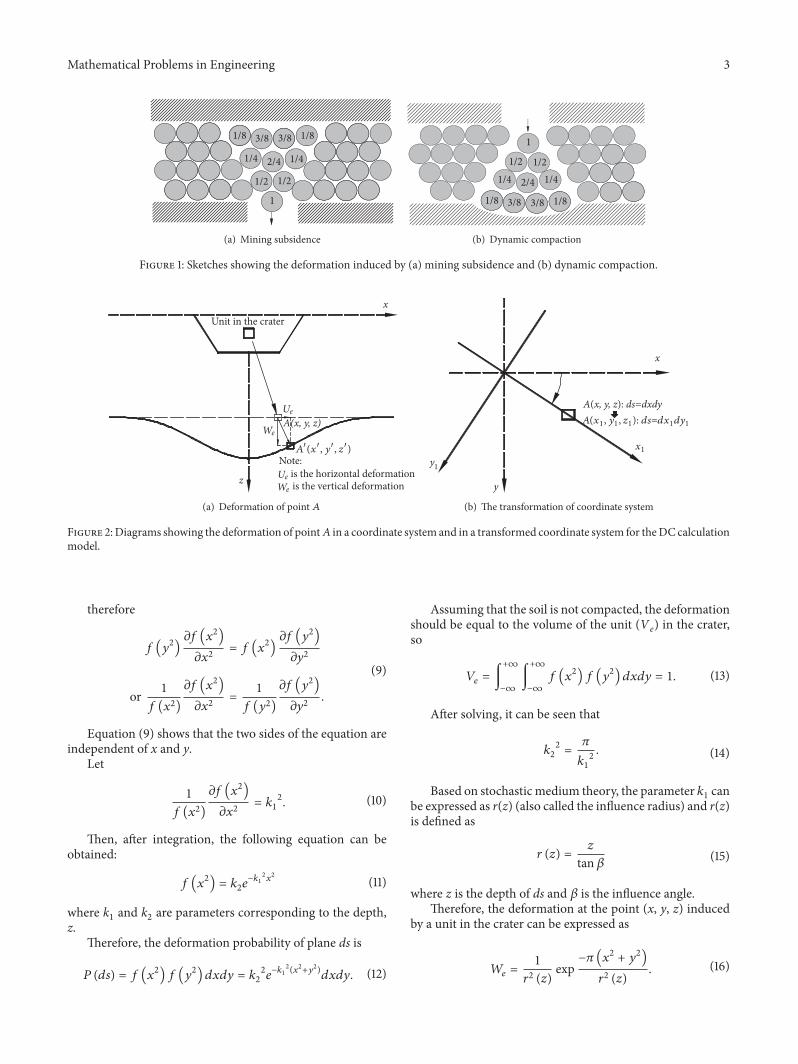
Stochastic medium theory was initially proposed byLitwiniszyn [20] and developed further by Liu et al. [21, 22].The stochastic medium in question is granular material likesand, gravel, and rock fragments. The excavation of under-ground space often causes deformation of the overlying strata[23, 24] and the theory is mainly used to calculate subsidenceafter an opening has been excavated. The subsidence causedby the excavation will be transferred to the overlying strata(Figure 1(a)). For DC, the settling is caused by the impactof the tamper. Figure 1(b) shows soil particles compressedby tamping. Comparing Figure 1(a) with Figure 1(b) showsthat the two kinds of settling are similar for noncohesivesoils.

In this paper, the deformation caused by the DC ismodeled using stochastic medium theory. A computational

model is proposed based on this theory and two parame-ters, a compression factor (determined by the type of DCequipment used) and an influence angle (a function of thesoil’s properties). Finally, the applicability of this model isexamined by comparing results calculated using the modelwith measurement made after a field test and with publisheddata. This study can provide a method for determining howwell a DC program is reinforcing the material upon which afoundationwill be installed andwill be valuable for the designand construction of DC projects.

2. Model for Dynamic Compaction

2.1. Introduction to Stochastic MediumTheory. In an Euleriancoordinate system, assume that the probability density fordeformation of dx is 𝑓(𝑥2) for the z-axis symmetry of thedeformation curve. The deformation probability P for dx canbe expressed as

𝑃 (𝑑𝑥) = 𝑓 (𝑥2) 𝑑𝑥. (2)

For an infinitesimal plane ds = dxdy centered at pointA(x,y,z), as shown in Figure 2(a), the deformation probabilityis

𝑃 (𝑑𝑠) = 𝑃 (𝑑𝑥) 𝑃 (𝑑𝑦) = 𝑓 (𝑥2) 𝑑𝑥𝑓 (𝑦2) 𝑑𝑦= 𝑓 (𝑥2) 𝑓 (𝑦2) 𝑑𝑠 (3)

If the coordinate system (x,y,z) is changed to (x1,y1,z) asshown in Figure 2(b), then (3) is transformed into

𝑃 (𝑑𝑠) = 𝑃 (𝑑𝑥1) 𝑃 (𝑑𝑦1) = 𝑓 (𝑥12) 𝑑𝑥𝑓 (𝑦12) 𝑑𝑦= 𝑓 (𝑥12) 𝑓 (𝑦12) 𝑑𝑠. (4)

If the x1 axis passes through the point A, then

𝑥12 = 𝑥2 + 𝑦2,𝑦1 = 0 (5)

𝑓 (𝑥12) 𝑓 (𝑦12) 𝑑𝑠 = 𝑓 (𝑥2 + 𝑦2) 𝑓 (0) 𝑑𝑠= 𝑐𝑓 (𝑥2 + 𝑦2) 𝑑𝑠 (6)

𝑓 (𝑥2) ⋅ 𝑓 (𝑦2) = 𝑓 (𝑥21) 𝑓 (𝑦21) = 𝑐 ⋅ 𝑓 (𝑥2 + 𝑦2) (7)

in which c is a constant.The derivation of (7) will yield:

𝑓 (𝑦2) 𝜕𝑓 (𝑥2)𝜕𝑥2 = 𝑐𝜕𝑓 (𝑥2 + 𝑦2)

𝜕 (𝑥2 + 𝑦2)𝜕 (𝑥2 + 𝑦2)

𝜕𝑥2= 𝑐𝜕𝑓 (𝑥2 + 𝑦2)

𝜕 (𝑥2 + 𝑦2)𝑓 (𝑥2) 𝜕𝑓 (𝑦2)

𝜕𝑦2 = 𝑐𝜕𝑓 (𝑥2 + 𝑦2)𝜕 (𝑥2 + 𝑦2)

𝜕 (𝑥2 + 𝑦2)𝜕𝑦2

= 𝑐𝜕𝑓 (𝑥2 + 𝑦2)𝜕 (𝑥2 + 𝑦2) ;

(8)

Mathematical Problems in Engineering 3

1/2

1

1/2 1/2

1/4 1/42/4

1/8 3/8 3/8 1/8

(a) Mining subsidence

1/2

1

1/2 1/21/4 1/42/4

1/8 3/8 3/8 1/8

(b) Dynamic compaction

Figure 1: Sketches showing the deformation induced by (a) mining subsidence and (b) dynamic compaction.

Unit in the crater

A(x, y, z)

x

z

Ue

Ue

We

We

Note:is the horizontal deformation is the vertical deformation

A(x, y, z)

(a) Deformation of point 𝐴

x

y

y1

x1

A(x, y, z): ds=dxdyA(x1, y1, z1): ds=dx1dy1

(b) The transformation of coordinate system

Figure 2:Diagrams showing the deformation of point𝐴 in a coordinate system and in a transformed coordinate system for theDC calculationmodel.

therefore

𝑓 (𝑦2) 𝜕𝑓 (𝑥2)𝜕𝑥2 = 𝑓 (𝑥2) 𝜕𝑓 (𝑦2)

𝜕𝑦2or 1𝑓 (𝑥2)

𝜕𝑓 (𝑥2)𝜕𝑥2 = 1𝑓 (𝑦2)

𝜕𝑓 (𝑦2)𝜕𝑦2 .

(9)

Equation (9) shows that the two sides of the equation areindependent of x and y.

Let

1𝑓 (𝑥2)𝜕𝑓 (𝑥2)𝜕𝑥2 = 𝑘12. (10)

Then, after integration, the following equation can beobtained:

𝑓 (𝑥2) = 𝑘2𝑒−𝑘12𝑥2 (11)

where k1 and k2 are parameters corresponding to the depth,z.

Therefore, the deformation probability of plane ds is

𝑃 (𝑑𝑠) = 𝑓 (𝑥2) 𝑓 (𝑦2) 𝑑𝑥𝑑𝑦 = 𝑘22𝑒−𝑘12(𝑥2+𝑦2)𝑑𝑥𝑑𝑦. (12)

Assuming that the soil is not compacted, the deformationshould be equal to the volume of the unit (Ve) in the crater,so

𝑉𝑒 = ∫+∞−∞

∫+∞−∞

𝑓 (𝑥2) 𝑓 (𝑦2) 𝑑𝑥𝑑𝑦 = 1. (13)

After solving, it can be seen that

𝑘22 = 𝜋𝑘12 . (14)

Based on stochastic medium theory, the parameter 𝑘1 canbe expressed as r(z) (also called the influence radius) and r(z)is defined as

𝑟 (𝑧) = 𝑧tan𝛽 (15)

where z is the depth of ds and 𝛽 is the influence angle.Therefore, the deformation at the point (x, y, z) induced

by a unit in the crater can be expressed as

𝑊𝑒 = 1𝑟2 (𝑧) exp−𝜋 (𝑥2 + 𝑦2)

𝑟2 (𝑧) . (16)

4 Mathematical Problems in Engineering

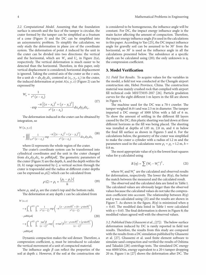
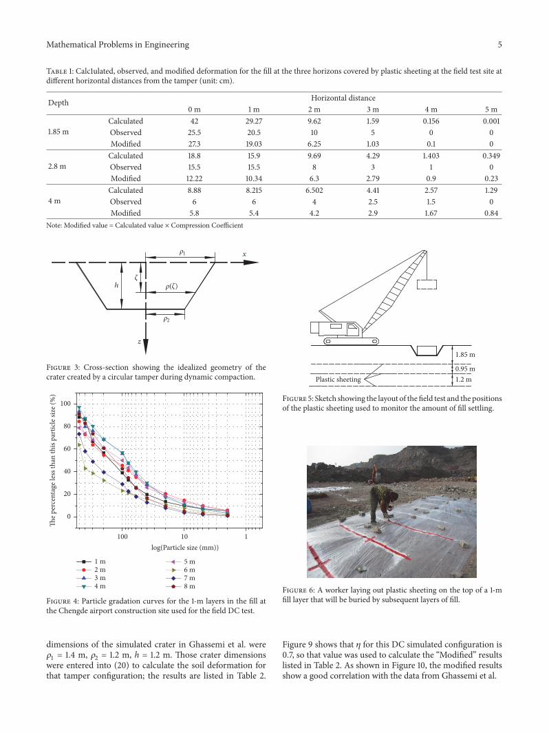
2.2. Computational Model. Assuming that the foundationsurface is smooth and the face of the tamper is circular, thecrater formed by the tamper can be simplified as a frustumof a cone (Figure 3) and the DC can be simplified intoan axisymmetric problem. To simplify the calculation, weonly study the deformation in plane zox of the coordinatesystem. The deformation of point A induced by the unit inthe crater can be divided into two directions: the verticaland the horizontal, which are We and 𝑈e in Figure 2(a),respectively. The vertical deformation is much easier to bedetected than the horizontal. Therefore, in this paper, onlyvertical displacement is considered; horizontal displacementis ignored. Taking the central axis of the crater as the z-axis,for a unit ds = dxedyedze centered at (xe, ye, ze) in the crater,the induced deformation at point A(x, y, z) (Figure 2) can beexpressed by

𝑊𝑒 = 1𝑟2 (𝑧 − 𝑧𝑒)⋅ exp −𝜋 [(𝑥 − 𝑥𝑒)2 + (𝑦 − 𝑦𝑒)2]𝑟2 (𝑧 − 𝑧𝑒) 𝑑𝑥𝑒𝑑𝑦𝑒𝑑𝑧𝑒.

(17)

The deformation induced in the crater can be obtained byintegration, so

𝑊(𝑥, 𝑦, 𝑧)= ∭

Ω

1𝑟2 (𝑧 − 𝑧𝑒) exp−𝜋 [(𝑥 − 𝑥𝑒)2 + (𝑦 − 𝑦𝑒)2]𝑟2 (𝑧 − 𝑧𝑒) 𝑑𝑥𝑒𝑑𝑦𝑒𝑑𝑧𝑒 (18)

where Ω represents the whole region of the crater.The crater’s coordinate system can be transformed into

cylindrical coordinates and the unit in the crater changedfrom 𝑑𝑥𝑒𝑑𝑦𝑒𝑑𝑧𝑒 to 𝜌𝑑𝜃𝑑𝜌𝑑𝜁. The geometric parameters ofthe crater (Figure 3) are the depth, h, and the depth within the(0, h) range represented by 𝜁; a vertical section through thecrater is trapezoidal and the radius at different crater depthscan be expressed as 𝜌(𝜁) which can be calculated from

𝜌 (𝜁) = 𝜌1 + (𝜌2 − 𝜌1) 𝜁ℎ (19)

where 𝜌1 and 𝜌2 are the crater’s top and the bottom radii.The deformation at any depth z can be calculated from

𝑊(𝑥, 𝑧)= 𝜂∫ℎ0∫𝜌(𝜁)0

∫2𝜋0

1𝑟2 (𝑧 − 𝜁) exp(−𝜋(𝑥 − 𝜌 cos 𝜃)2 + (0 − 𝜌 sin 𝜃)2𝑟2 (𝑧 − 𝜁) )

⋅ 𝜌𝑑𝜃𝑑𝜌𝑑𝜁= 𝜂∫ℎ0∫𝜌(𝜉)0

∫2𝜋0

tan2𝛽(𝑧 − 𝜁)2 exp(−𝜋 tan2𝛽(𝑥 − 𝜌 cos 𝜃)2 + (𝜌 sin 𝜃)2

(𝑧 − 𝜁)2 )⋅ 𝜌𝑑𝜃𝑑𝜌𝑑𝜁

(20)

Dynamic compaction makes the soil denser. Therefore, acompression coefficient, 𝜂, must be introduced to calculatethe vertical movement of a unit of compacted material.

The influence angle 𝛽 can reflect the properties of thesoil at depth z. However, if the soil at the construction site

is considered to be homogeneous, the influence angle will beconstant. For DC, the impact energy influence angle is themain factor affecting the amount of compaction. Therefore,the impact energy influence angle𝛽 is used in the calculationsin this paper. According to Yao [25], the DC impact influenceangle for gravelly soil can be assumed to be 30∘ from thehorizontal, so 30∘ is used as the influence angle in all thecalculations presented below. The subsidence at a specificdepth can be calculated using (20); the only unknown is 𝜂,the compression coefficient.

3. Model Verification

3.1. Field Test Results. To acquire values for the variables inthe model, a field test was conducted at the Chengde airportconstruction site, Hebei Province, China. The constructionmaterial was mainly crushed rock that complied with airportfill technical code MH/T5035-2017 [26]. Particle gradationcurves for the eight different 1-m layers in the fill are shownin Figure 4.

The machine used for the DC was a 70-t crawler. Thetamper weighed 16.8 t and was 2.5 m in diameter.The tamperimparted a DC energy of 1000 kNm with a fall of 6 m.To show the amount of settling in the different fill layerscaused by theDC, thin plastic sheeting was laid down at threedifferent horizons as the fill was being placed. The sheetingwas installed at depths of 1.85 m, 2.8 m, and 4 m belowthe final fill surface as shown in Figures 5 and 6. For thecalculations below, the geometry of the crater was simplifiedto make the crater a cylinder with a radius of 1.2 m and theparameters used in the calculations were 𝜌1 = 𝜌2 = 1.2 m, h =0.8 m.

Themost appropriate value of 𝜂 is the lowest least squaresvalue for 𝜂 calculated using

𝑅 (𝜂) = ∑(𝑊𝑖 − 𝑊∗𝑖 )2 , (21)

where𝑊𝑖 and𝑊∗𝑖 are the calculated and observed resultsfor deformation, respectively. The lower the 𝑅(𝜂), the betterthe match between the measured and the calculated result.

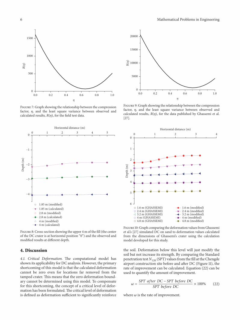
The observed and the calculated data are listed in Table 1.The calculated values are obviously larger than the observedvalues because the calculated values do not take the compres-sion coefficient into account. The relationship between 𝑅(𝜂)and 𝜂 was calculated using (21) and the results are shown inFigure 7. As shown in the figure, 𝑅(𝜂) is minimized when 𝜂= 0.65. The modified data listed in Table 1 were calculatedwith 𝜂 = 0.65.The final deformation is shown in Figure 8; themodified values agreed well with the observed values.

3.2. PublishedData (Ghassemi et al., [27]). Thebelow-surfacedeformation induced by DC is rarely reported in field testresults. Therefore, the results from this study are comparedwith the results from aDC simulation published byGhassemiet al. [27]. Ghassemi et al. used finite element software tosimulate sand compaction and verified the results of Oshimaand Takada’s [28] centrifuge tests. The simulated DC energywas 4000 kNm, energy equivalent to a 20-t tamper dropping20 m. Figure 1 in [27] shows the deformation after DC. The

Mathematical Problems in Engineering 5

Table 1: Calc1ulated, observed, and modified deformation for the fill at the three horizons covered by plastic sheeting at the field test site atdifferent horizontal distances from the tamper (unit: cm).

Depth Horizontal distance0 m 1 m 2 m 3 m 4 m 5 m

1.85 mCalculated 42 29.27 9.62 1.59 0.156 0.001Observed 25.5 20.5 10 5 0 0Modified 27.3 19.03 6.25 1.03 0.1 0

2.8 mCalculated 18.8 15.9 9.69 4.29 1.403 0.349Observed 15.5 15.5 8 3 1 0Modified 12.22 10.34 6.3 2.79 0.9 0.23

4 mCalculated 8.88 8.215 6.502 4.41 2.57 1.29Observed 6 6 4 2.5 1.5 0Modified 5.8 5.4 4.2 2.9 1.67 0.84

Note: Modified value = Calculated value × Compression Coefficient

x

h

1

2

z

()

Figure 3: Cross-section showing the idealized geometry of thecrater created by a circular tamper during dynamic compaction.

1 m2 m3 m4 m

5 m6 m7 m8 m

0

20

40

60

80

100

The p

erce

ntag

e les

s tha

n th

is pa

rtic

le si

ze (%

)

10 1100log(Particle size (mm))

Figure 4: Particle gradation curves for the 1-m layers in the fill atthe Chengde airport construction site used for the field DC test.

dimensions of the simulated crater in Ghassemi et al. were𝜌1 = 1.4 m, 𝜌2 = 1.2 m, h = 1.2 m. Those crater dimensionswere entered into (20) to calculate the soil deformation forthat tamper configuration; the results are listed in Table 2.

1.85 m

0.95 mPlastic sheeting 1.2 m

Figure 5: Sketch showing the layout of the field test and the positionsof the plastic sheeting used to monitor the amount of fill settling.

Figure 6: A worker laying out plastic sheeting on the top of a 1-mfill layer that will be buried by subsequent layers of fill.

Figure 9 shows that 𝜂 for this DC simulated configuration is0.7, so that value was used to calculate the “Modified” resultslisted in Table 2. As shown in Figure 10, the modified resultsshow a good correlation with the data from Ghassemi et al.

6 Mathematical Problems in Engineering

0

500

R(

)

1000

1500

0.2 0.4 0.6 0.8 1.00.0

Figure 7: Graph showing the relationship between the compressionfactor, 𝜂, and the least square variance between observed andcalculated results, 𝑅(𝜂), for the field test data.

1.85 m (modified) 1.85 m (calculated) 2.8 m (modified) 2.8 m (calculated) 4 m (modified) 4 m (calculated)

0 1 2 3 4 5Horizontal distance (m)

−4

−3

−2

−1

0

Dep

th (m

)

Figure 8: Cross-section showing the upper 4m of the fill (the centerof the DC crater is at horizontal position “0”) and the observed andmodified results at different depth.

4. Discussion

4.1. Critical Deformation. The computational model hasshown its applicability for DC analysis. However, the primaryshortcoming of this model is that the calculated deformationcannot be zero even for locations far removed from thetamped crater. This means that the zero deformation bound-ary cannot be determined using this model. To compensatefor this shortcoming, the concept of a critical level of defor-mation has been formulated.The critical level of deformationis defined as deformation sufficient to significantly reinforce

0

5000

R()

10000

15000

20000

0.2 0.4 0.6 0.8 1.00.0

Figure 9: Graph showing the relationship between the compressionfactor, 𝜂, and the least square variance between observed andcalculated results, 𝑅(𝜂), for the data published by Ghassemi et al.[27].

1.6 m (GHASSEMI) 1.6 m (modified)2.4 m (GHASSEMI) 2.4 m (modified)3.2 m (GHASSEMI) 3.2 m (modified)4 m (GHASSEMI) 4 m (modified)4.8 m (GHASSEMI) 4.8 m (modified)

0 1 2 3 4Horizontal distance (m)

6

5

4

3

2

1

0

Dep

th (m

)

Figure 10:Graph comparing the deformation values fromGhassemiet al.’s [27] simulated DC on sand to deformation values calculatedfrom the dimensions of Ghassemi’s crater using the calculationmodel developed for this study.

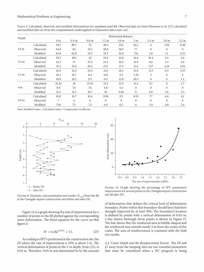
the soil. Deformation below this level will just modify thesoil but not increase its strength. By comparing the Standardpenetration testN120 (SPT) values from the fill at theChengdeairport construction site before and after DC (Figure 11), therate of improvement can be calculated. Equation (22) can beused to quantify the amount of improvement.

𝜔 = 𝑆𝑃𝑇 𝑎𝑓𝑡𝑒𝑟 𝐷𝐶 − 𝑆𝑃𝑇 𝑏𝑒𝑓𝑜𝑟𝑒 𝐷𝐶𝑆𝑃𝑇 𝑏𝑒𝑓𝑜𝑟𝑒 𝐷𝐶 × 100% (22)

where 𝜔 is the rate of improvement.

Mathematical Problems in Engineering 7

Table 2: Calculated, observed, and modified deformations for simulated sand fill. Observed data are from Ghassemi et al. [27]; calculatedand modified data are from the computational model applied to Ghassemi’s data (unit: cm).

Depth Horizontal distance0 m 0.4 m 0.8 m 1.2 m 1.6 m 2 m 2.4 m 2.8 m 3.2 m

1.6 mCalculated 94.1 89.7 75 49.3 24.1 10.2 4 1.58 0.48Observed 64.6 64 55.1 40.8 18.9 7.7 0 0 0Modified 65.8 62.8 52.5 34.5 16.9 7.14 2.8 1.1 0.33

2.4 mCalculated 50.3 48.1 42 33.6 24.6 16.6 10.4 6.1 2.6Observed 42.5 37 33.4 25.4 18.3 13.9 8.6 5.3 4.6Modified 35.2 33.6 29.4 23.5 17.3 11.6 7.27 4.26 1.84

3.2 mCalculated 26.8 26.2 24.4 21.6 18.3 14.8 11.5 8.5 4.55Observed 20.3 19.7 16.1 11.8 5.9 5.39 3 0 0Modified 18.8 18.3 17.1 15.1 12.8 10.4 8 6 3.2

4 mCalculated 16.26 16 15.35 14.3 12.9 11.4 9.7 8 4.7Observed 8.9 7.6 7.6 4.8 4.4 0 0 0 0Modified 11.4 11.2 10.7 10 9.06 8 6.8 5.6 3.3

4.8 mCalculated 10.8 10.7 10.4 9.94 9.3 8.55 7.7 6.8 4.1Observed 7 6 6 0 0 0 0 0 0Modified 7.56 7.5 7.3 6.9 6.5 6 5.4 4.8 2.9

Note: Modified value = Calculated value × Compression Coefficient

Before DC After DC

0 4 8 12 16 20N120

7

6

5

4

3

2

1

0

Dep

th (m

)

Figure 11: Dynamic cone penetration test results (N120) from the fillat the Chengde airport construction site before and after DC.

Figure 12 is a graph showing the rate of improvement for anumber of points in the fill plotted against the correspondinginner deformation. The fitted equation for the curve on thatfigure is

𝑊 = 0.28𝑒𝜔/0.65 + 3.5. (23)

According to SPT’s performed at the construction site, theDI where the rate of improvement is 50% is about 5 m. Thevertical deformation of points at the 5-m depth, from (22), is0.04 m. Therefore, 0.04 m was determined to be the amount

0

20

40

60

Inne

r def

orm

atio

n (c

m)

0.0 0.5 1.0 1.5 2.0 2.5 3.0 3.5−0.5The rate of improvement(×100%)

Figure 12: Graph showing the percentage of SPT penetrationimprovement for several points in the Chengde airport constructionsite fill after DC.

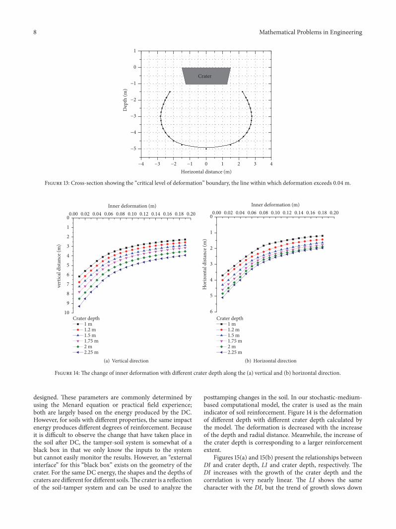
of deformation that defines the critical level of deformationboundary. Points within that boundary should have had theirstrength improved by at least 50%. The boundary’s locationis defined by points with a vertical deformation of 0.04 m;a line drawn thorough those points is shown in Figure 13.The line shows that the reinforced area is bubble-shaped andthe reinforced area extends nearly 3 m from the center of thecrater. The area of reinforcement is consisted with the fieldtest results.

4.2. Crater Depth and the Reinforcement Extent. The DI andLI away from the tamping sites are two essential parametersthat must be considered when a DC program is being

8 Mathematical Problems in Engineering

Crater

−5

−4

−3

−2

−1

0

1

Dep

th (m

)

210 3 4−2−3 −1−4Horizontal distance (m)

Figure 13: Cross-section showing the “critical level of deformation” boundary, the line within which deformation exceeds 0.04 m.

Crater depth1 m1.2 m1.5 m1.75 m2 m2.25 m

0.00 0.02 0.04 0.06 0.08 0.10 0.12 0.14 0.16 0.18 0.20Inner deformation (m)

10

9

8

7

6

5

4

3

2

1

0

vert

ical

dist

ance

(m)

(a) Vertical direction

Crater depth1 m1.2 m1.5 m1.75 m2 m2.25 m

0.00 0.02 0.04 0.06 0.08 0.10 0.12 0.14 0.16 0.18 0.20Inner deformation (m)

6

5

4

3

2

1

0

Hor

izon

tal d

istan

ce (m

)

(b) Horizontal direction

Figure 14: The change of inner deformation with different crater depth along the (a) vertical and (b) horizontal direction.

designed. These parameters are commonly determined byusing the Menard equation or practical field experience;both are largely based on the energy produced by the DC.However, for soils with different properties, the same impactenergy produces different degrees of reinforcement. Becauseit is difficult to observe the change that have taken place inthe soil after DC, the tamper-soil system is somewhat of ablack box in that we only know the inputs to the systembut cannot easily monitor the results. However, an “externalinterface” for this “black box” exists on the geometry of thecrater. For the same DC energy, the shapes and the depths ofcraters are different for different soils.The crater is a reflectionof the soil-tamper system and can be used to analyze the

posttamping changes in the soil. In our stochastic-medium-based computational model, the crater is used as the mainindicator of soil reinforcement. Figure 14 is the deformationof different depth with different crater depth calculated bythe model. The deformation is decreased with the increaseof the depth and radial distance. Meanwhile, the increase ofthe crater depth is corresponding to a larger reinforcementextent.

Figures 15(a) and 15(b) present the relationships betweenDI and crater depth, LI and crater depth, respectively. TheDI increases with the growth of the crater depth and thecorrelation is very nearly linear. The LI shows the samecharacter with the DI, but the trend of growth slows down

Mathematical Problems in Engineering 9

4

5

6

7

8

9

10D

I (m

)

1.0 1.5 2.0 2.5 3.00.5Crater Depth (m)

(a) DI

2.0

2.5

3.0

3.5

4.0

4.5

5.0

LI (m

)

1.0 1.5 2.0 2.5 3.00.5Crater Depth (m)

(b) LI

Figure 15: The relationship of crater depth and (a) DI, depth of soil improvement, and (b) LI, lateral extent of soil improvement.

with the increase of crater depth. When the crater depthincreases from 1 m to 2 m, the growth of LI is about 1.2m. However, the growth of LI is just 0.6 m when the craterdepth increases from 2 m to 3 m. Therefore, it can beconcluded that, increasing the crater depth, the DI can besignificantly expanded while LI increases consistently with aslowly decreasing rate (Figure 15(b)).

5. Conclusions

A computational model based on stochastic medium the-ory has been developed to determine how much dynamiccompaction (DC) reinforces the soil. This model is verifiedby comparing model results with the results from twocompaction programs, one on crushed rock fill and theother simulating a sand fill. The compression coefficientsfor these two programs are 0.65 for the crushed rock and0.7 for the sand. This method for establishing the degree ofreinforcement has several advantages when compared withtraditional methods. First, it takes the geometry of the craterinto account. The shape and depth of the crater can reflectthe DC energies and the soil properties and the crater’sdimension are easy to obtain at the construction site withno special equipment or personnel training required. Second,the model assesses the extent of the reinforcement bothlaterally and vertically instead of merely estimating the DI.Finally, the computation is simple and can be easily solvedusing commercially available programs. However, this modelis a prototype and more details should be studied. Additionalvalidation of the computational model is also needed beforesufficient confidence on themodel’s results can be established.

Data Availability

The data used to support the findings of this study areavailable from the corresponding author upon request.

Conflicts of Interest

The authors declare no conflicts of interest.

Acknowledgments

This research was supported by the National Basic ResearchProgram of China, grant number 2014CB047004. We thankDavid Frishman, Ph.D0, from Liwen Bianji, Edanz Group,China, for editing the English text of a draft of thismanuscript.

References

[1] Y.Wang, P. Guo, F. Dai, X. Li, Y. Zhao, and Y. Liu, “Behavior andmodeling of fiber-reinforced clay under triaxial compressionby combining the superposition method with the energy-basedhomogenization technique,” International Journal of Geome-chanics, vol. 18, no. 12, Article ID 04018172, 2018.

[2] Y.Wang, P. Guo, X. Li, H. Lin, Y. Liu, and H. Yuan, “Behavior offiber-reinforced and lime-stabilized clayey soil in triaxial tests,”Applied Sciences, vol. 9, no. 5, Article ID 900, 2019.

[3] Y. X. Wang, P. P. Guo, H. Lin et al., “Numerical analysis offiber-reinforced soils based on the equivalent additional stressconcept,” International Journal of Geomechanics, 2019.

[4] Z. Ma, F. Dang, and H. Liao, “Numerical study of the dynamiccompaction of gravel soil ground using the discrete elementmethod,” Granular Matter, vol. 16, no. 6, pp. 881–889, 2014.

[5] S.-J. Feng, K. Tan, W.-H. Shui, and Y. Zhang, “Densification ofdesert sands by high energy dynamic compaction,” EngineeringGeology, vol. 157, pp. 48–54, 2013.

[6] L. Menard and Y. Broise, “Theoretical and practical aspects ofdynamic consolidation,” Geotechnique, vol. 25, no. 1, pp. 3–18,1975.

[7] W.-L. Zou, Z. Wang, and Z.-F. Yao, “Effect of dynamic com-paction on placement of high-road embankment,” Journal ofPerformance of Constructed Facilities, vol. 19, no. 4, pp. 316–323,2005.

10 Mathematical Problems in Engineering

[8] P.W.Mayne, J. S. Jones Jr., and J. C.Dumas, “Ground response todynamic compaction,” Journal of Geotechnical Engineering, vol.110, no. 6, pp. 757–774, 1984.

[9] G. A. Leonards, W. A. Cutter, and R. D. Holtz, “Dynamiccompaction of granular soils,” Journal of the GeotechnicalEngineering Division, vol. 106, no. 1, pp. 35–44, 1980.

[10] R. G. Lukas, “Dynamic compaction for highway construction,Design and construction guidelines, Volume I,” Federal High-way Administration Report FHWA-RD-86-133, 1986.

[11] K. M. Rollins and J. Kim, “Dynamic compaction of collapsiblesoils based on U.S. case histories,” Journal of Geotechnical andGeoenvironmental Engineering, vol. 136, no. 9, pp. 1178–1186,2010.

[12] B. C. Slocombe, Dynamic Compaction. Ground Improvement,vol. 2, Glasgow, Chapman & Hall. Cap., 1993.

[13] V. Luongo, “Dynamic compaction: predicting depth ofimprovement,” Grouting, Soil Improvement and Geosynthetics,ASCE, pp. 27–939, 1992.

[14] Y. K. Chow, D. M. Yong, K. Y. Yong, and S. L. Lee, “Dynamiccompaction of loose sand deposits,” Soils and Foundations, vol.32, no. 4, pp. 93–106, 1992.

[15] M. T. Smits and L. De Quelerij, “The effect of dynamic com-paction on dry granular soils,” inProceedings of the InternationalConference on Soil Mechanics and Foundation Engineering, 12th,vol. 2, Rio de Janiero, Brazil, 1989.

[16] C. J. Poran and J. A. Rodriguez, “Finite element analysis ofimpact behavior of sand,” Soils and Foundations, vol. 32, no. 4,pp. 68–80, 1992.

[17] F. H. Lee and Q. Gu, “Method for estimating dynamic com-paction effect on sand,” Journal of Geotechnical and Geoenviron-mental Engineering, vol. 130, no. 2, pp. 139–152, 2004.

[18] K. F. Mostafa and R. Y. Liang, “Numerical modeling of dynamiccompaction in cohesive soils,” in Proceedings of the Geo-Frontiers Congress 2011, pp. 738–747, Dallas, Texas, UnitedStates, 2011.

[19] M. Jia, Y. Yang, B. Liu, and S. Wu, “PFC/FLAC coupledsimulation of dynamic compaction in granular soils,” GranularMatter, vol. 32, no. 4, Article ID 76, 2018.

[20] J. Litwiniszyn, “The theories and model research of movementsof ground masses,” in Proceedings of the European CongressGround Movement, pp. 203–209, Leeds, UK, 1957.

[21] B. C. Liu, “Ground surface movements due to undergroundexcavation in the People’s Republic of China,” Excavation,Support and Monitoring, pp. 781–817, 1993.

[22] J. S. Yang, B. C. Liu, and M. C. Wang, “Modeling of tunneling-induced ground surface movements using stochastic mediumtheory,” Tunnelling and Underground Space Technology, vol. 19,no. 2, pp. 113–123, 2004.

[23] P. Guo, X. Gong, and Y. Wang, “Displacement and forceanalyses of braced structure of deep excavation consideringunsymmetrical surcharge effect,” Computers & Geosciences, vol.113, Article ID 103102, 2019.

[24] Y. Wang, S. Shan, C. Zhang, and P. Guo, “Seismic responseof tunnel lining structure in a thick expansive soil stratum,”Tunnelling and Underground Space Technology, vol. 88, pp. 250–259, 2019.

[25] Y. P. Yao and B. Z. Zhang, “Reinforcement range of dynamiccompaction based on volumetric strain,” Rock and Soil Mechan-ics, vol. 9, Article ID 032, 2016 (Chinese).

[26] MH/T5035-2017, “Technical code for high filling engineeringof airport,” Civil Aviation Administration of China, 2017 (Chi-nese).

[27] A. Ghassemi, A. Pak, and H. Shahir, “A numerical tool fordesign of dynamic compaction treatment in dry and moistsands,” Iranian Journal of Science & Technology, Transaction B:Engineering, vol. 33, no. 4, pp. 313–326, 2009.

[28] A. Oshima and N. Takada, “Relation between compacted areaand ram momentum by heavy tamping,” in Proceedings ofthe International Conference on Soil Mechanics and FoundationEngineering-International Society for Soil Mechanics and Foun-dation Engineering, AA BALKEMA, vol. 3, pp. 1641–1644, 1997.

Hindawiwww.hindawi.com Volume 2018

MathematicsJournal of

Hindawiwww.hindawi.com Volume 2018

Mathematical Problems in Engineering

Applied MathematicsJournal of

Hindawiwww.hindawi.com Volume 2018

Probability and StatisticsHindawiwww.hindawi.com Volume 2018

Journal of

Hindawiwww.hindawi.com Volume 2018

Mathematical PhysicsAdvances in

Complex AnalysisJournal of

Hindawiwww.hindawi.com Volume 2018

OptimizationJournal of

Hindawiwww.hindawi.com Volume 2018

Hindawiwww.hindawi.com Volume 2018

Engineering Mathematics

International Journal of

Hindawiwww.hindawi.com Volume 2018

Operations ResearchAdvances in

Journal of

Hindawiwww.hindawi.com Volume 2018

Function SpacesAbstract and Applied AnalysisHindawiwww.hindawi.com Volume 2018

International Journal of Mathematics and Mathematical Sciences

Hindawiwww.hindawi.com Volume 2018

Hindawi Publishing Corporation http://www.hindawi.com Volume 2013Hindawiwww.hindawi.com

The Scientific World Journal

Volume 2018

Hindawiwww.hindawi.com Volume 2018Volume 2018

Numerical AnalysisNumerical AnalysisNumerical AnalysisNumerical AnalysisNumerical AnalysisNumerical AnalysisNumerical AnalysisNumerical AnalysisNumerical AnalysisNumerical AnalysisNumerical AnalysisNumerical AnalysisAdvances inAdvances in Discrete Dynamics in

Nature and SocietyHindawiwww.hindawi.com Volume 2018

Hindawiwww.hindawi.com

Di�erential EquationsInternational Journal of

Volume 2018

Hindawiwww.hindawi.com Volume 2018

Decision SciencesAdvances in

Hindawiwww.hindawi.com Volume 2018

AnalysisInternational Journal of

Hindawiwww.hindawi.com Volume 2018

Stochastic AnalysisInternational Journal of

Submit your manuscripts atwww.hindawi.com