defining the use of a resting and migratory area for

1

Defining the use of a resting and migratory area for baleen whales in a key

habitat (Geographe Bay) in Australia’s south-west

June, 2014

Prepared by Chandra Salgado Kent1, Chris Burton2, Angela Recalde-Salas1, Sarah Marley1, and Eric Kniest3

1Centre for Marine Science and Technology (CMST), Curtin University, GPO Box U 1987 Perth 6845, WA

2Western Whale Research, P.O. Box 1076, Dunsborough, WA 6281 3University of Newcastle, University Drive, Callaghan NSW 2308

Submitted to the International Fund for Animal Welfare

PROJECT CMST 1199

REPORT 2014-35 Contents

2

DEFINING THE USE OF A RESTING AND MIGRATORY AREA FOR BALEEN WHALES IN A KEY HABITAT (GEOGRAPHE BAY) IN AUSTRALIA’S SOUTH-WEST ........................................... 1

EXECUTIVE SUMMARY .......................................................................................................................... 6

1. INTRODUCTION............................................................................................................................ 10

2. METHODS ...................................................................................................................................... 10

2.1. OBSERVATION AND MEASUREMENT PLATFORMS ....................................................................................... 11

3. RESULTS ....................................................................................................................................... 19

3.1. ABUNDANCE OF BALEEN WHALES OVER THE PEAK OF THE BLUE WHALE MIGRATION PERIOD ............................... 19 3.2. CHANGES IN THE SOUNDSCAPE ENVIRONMENT DURING THE PEAK OF THE BLUE WHALE MIGRATION .................... 33 3.3. DISTURBANCE DURING THE PEAK OF THE BLUE WHALE SEASON .................................................................... 49

4. DISCUSSION AND CONCLUSIONS ........................................................................................... 50

4.1. ABUNDANCE ESTIMATIONS .................................................................................................................. 50 4.2. ACOUSTIC ANALYSIS ........................................................................................................................... 52 4.3. VESSEL INTERACTIONS ......................................................................................................................... 52

REFERENCES ........................................................................................................................................ 53

APPENDIX A: DATA ARCHIVING ....................................................................................................... 55

APPENDIX B: HEALTH SAFETY AND ENVIRONMENT AND PERMITS AND ETHICS APPROVALS .......................................................................................................................................... 55

APPENDIX C: PERSONNEL ................................................................................................................. 55

LIST OF PERSONNEL IN THE 2013 FIELD SEASON .................................................................................................... 55

APPENDIX D. PUBLICITY, MEDIA INTERACTION AND COMMUNITY ENGAGEMENT ............. 56

VISITORS ........................................................................................................................................................ 58

3

Table of Figures Figure 1. Approximate positions of acoustic recordings made by a noise logger (dark blue

circle), and the theodolite observation station (orange circle) with approximate detection ranges out to ~4 km where whale surfacings are expected to have a high probability of being detected (dashed orange line) and to ~9 km where maximum detection range is expected (dotted orange lines) within Geographe Bay. The black arrows indicate typical migration routes of whales migrating south along the coast of Australia on route to feeding grounds. .................................................................................................................................................................. 11

Figure 2. Four acoustic loggers and their moorings packed for transportation to Geographe Bay from Perth, Western Australia.............................................................................................................. 12

Figure 3. Locations of the acoustic loggers (green circles) deployed off Pt. Piquet, Geographe Bay (Western Australia) in 2013. Central acoustic logger position was the approximate position of acoustic loggers deployed in previous years.................................................................... 13

Figure 4. Land-based hill observation team. Depicted in the photos are: (A) two spotters and the theodolite operator, and (B) a spotter, the theodolite operator and the computer operator running Vadar software. ............................................................................................................... 15

Figure 5. Example of whale, vessel, and dolphin observations and tracks displayed in real time in Vadar over a ~4 hour period on the 21 November 2013 (pods are labelled with letters and have a blow or breach icon, and vessels are labelled with numbers). .................. 16

Figure 6. Diagram showing observer placement on vessel during surveys. .................................... 17 Figure 7. (A) Study area (shaded in red) with transects design (using Distance 6.0 and ArcGIS

10.0) to provide optimal transect travel time and coverage (~2km half strip width). (B) Transect lines plotted for inputting into vessel GPS. ........................................................................... 18

Figure 8. Distribution of humpback whale sightings (including positions of all surfacings captured with the theodolite of groups tracked) between 2010 and 2013. .............................. 20

Figure 9. Distribution of blue whale sightings (including positions of all surfacings captured with the theodolite of groups tracked) between 2010 and 2013. .................................................. 21

Figure 10. Total number of humpback (left panels) and blue (right panels) whales detected from the land-based platform during 2010, 2011, 2012 and 2013 field season. ..................... 22

Figure 11. Average number of humpback (left panels) and blue (right panels) whales detected per hour from the land-based platform during 2010, 2011, 2012 and 2013 field season. .. 23

Figure 12. Average number of humpback (left panels) and blue (right panels) whales detected per hour from the land-based platform over the survey field seasons during 2010, 2011, 2012 and 2013. .................................................................................................................................................... 24

Figure 13. Humpback whale abundance counts corrected for hours in a day (points), and estimated across unsurveyed days using a spline interpolation (dashed line) using Generalized Cross Validation (GCV) to assign a value for the parameter lambda. 95% confidence Intervals are indicated with the upper and lower dotted lines. Total estimate number of is indicated in the right hand upper corner of each figure. ......................................... 26

Figure 14. Blue whale abundance counts corrected for hours in a day (points), and estimated across unsurveyed days using a spline interpolation (dashed line) using Generalized Cross Validation (GCV) to assign a value for the parameter lambda. 95% confidence Intervals are indicated with the upper and lower dotted lines. Total estimate number of is indicated in the right hand upper corner of each figure. ............................................................................................. 26

Figure 15. Photos showing observers on the 5m Zodiac during surveys. ......................................... 27 Figure 16. Plot of weather conditions during main field work period and during vessel

surveys. Bars in blue and red are based in data collected from two weather stations close to the study area (daily average), bars in green are qualitative wind speed estimations made from the vessel. Wind speeds (mean knots) for each of the 5 surveys. .......................... 28

Figure 17. Map showing coverage of vessel surveys in relation to land-based observations in 2013, using the vessel survey track (dark blue circles) from the 16th of November 2013 as

4

an example of a typical track overlayed by land-based observations of surfacing groups of whales (light blue circles). .............................................................................................................................. 29

Figure 18. Example of boat tracks (dark blue) overlayed by positions at first detection of animals on a single survey day (16th of November 2013). Positions were calculated from the distance down from the horizon to the animals using photographs. .................................... 31

Figure 19. Percentages of sighting cues. ......................................................................................................... 32 Figure 20. (A) Blue whale left dorsal (LD) photo taken during Trip 12, and (B) blue whale LD

photo taken during Trip 13. ........................................................................................................................... 32 Figure 21. Power spectrum density of ambient noise averaged over 6-hour periods between

12 am and 12 pm of no wind (blue), high wind (green), and the maximum vessel noise (red) during one day in December 2008. The dotted lines show the standard deviation of fluctuations at different frequencies........................................................................................................... 34

Figure 22. Spectrogram of sea noise recorded on LF GB2008 over the first (top panel) and second (bottom panel) ten day periods of passive acoustic recording in Geographe Bay in 2008................................................................................................................................................................. ......... 35

Figure 23. Spectrogram of sea noise recorded on LF GB2008 over the third (top panel) and forth (bottom panel) ten day periods of passive acoustic recording in Geographe Bay in 2008.......................................................................................................................................................................... 36

Figure 24. Spectrogram of sea noise recorded on LF GB2010 over the first (top panel) and second (bottom panel) ten day periods of passive acoustic recording in Geographe Bay in 2010.......................................................................................................................................................................... 37

Figure 25. Spectrogram of sea noise recorded on LF GB2010 over the last eleven day period of passive acoustic recording in Geographe Bay in 2010. ....................................................................... 38

Figure 26. Spectrogram of sea noise recorded on LF 3070 over the first ten day period (top panel) of passive acoustic recording, and spectrogram (bottom, left panel) and waveform (bottom, right panel) of blue whale song recorded on the 17th of November 2011 at 09:05 in Geographe Bay. ............................................................................................................................................... 39

Figure 27. Spectrogram of sea noise recorded on LF 3070 over the second ten day period (top panel) and the last three (bottom panel) of passive acoustic recording in Geographe Bay in 2011................................................................................................................................................................. ......... 40

Figure 28. Spectrogram of sea noise recorded on LF 3186 over the first ten day period (top panel) of passive acoustic recording in Geographe Bay in 2012; spectrogram (left, middle panel) and waveform (right, middle panel) of blue whale non-song sounds produced on the 9th of November 2012 at 20:37; high time-resolution spectrograms of two of the non-song sounds from the middle panels (bottom panels). ....................................................................... 41

Figure 29. Spectrogram of sea noise recorded on LF 3186 over the second (top panel) and third (bottom panel) ten day periods of passive acoustic recording in Geographe Bay in 2012................................................................................................................................................................. ......... 42

Figure 30. Spectrogram of sea noise recorded on LF 3186 over the last ten day period of passive acoustic recording in Geographe Bay in 2012 (recordings after the 22nd are in air after recovery of the acoustic logger). ....................................................................................................... 43

Figure 31. Spectrogram of sea noise recorded on LF 3269 over the first ten day period (top panel) of passive acoustic recording in Geographe Bay in 2013, and spectrogram (left, bottom panel) and waveform (right, bottom panel) of example of multiple humpback whale songs produced simultaneiously on the 19th of November at 15:00. .............................. 44

Figure 32. Spectrogram (left panel) and waveform (right panel) of a recreational vessel recorded on the 20th of November 2013 at 15:00 in Geographe Bay. .......................................... 45

Figure 33. Spectrogram of sea noise recorded on LF 3269 over the second (top panel) and third (bottom panel) ten-day periods of passive acoustic recording in Geographe Bay in 2013.......................................................................................................................................................................... 46

Figure 34. Spectrogram of sea noise recorded on LF 3269 over the last ten-day periods of passive acoustic recording in Geographe Bay in 2013. ....................................................................... 47

Figure 35. Number of blue whales detected vocalising per day (in 2011, 2012, and 2013). .... 48

5

Figure 36. The percentage of blue whale groups of different group composition types observed during land-based observations in Geographe Bay (blue bars) during 2010, 2011, 2012, and 2013, and the percentage in each group composition category involved in one or more vessel interactions (red bars). ............................................................................................. 49

Figure 37. The number of pygmy blue whale groups involved in no interactions (0), interactions with one vessel (1), with two vessels (2), and with three vessels (3) during their use of Geographe Bay during land-based observations in 2010, 2011, 2012, and 2013................................................................................................................................................................. ......... 50

Figure 39. Screen capture of SouWEST blog featuring IFAW support. ............................................... 56 Figure 40. SouWEST blog visitation statistics. .............................................................................................. 57

Table of Tables

Table 1. Summary of sea noise logger deployment for all years. Times are those in WA (UTC + 8 hours). ......................................................................................................................................................... 13 Table 2. Noise logger settings and sampling regimes for all years of recording. ........................... 14 Table 3. Summary of land-based hill observation effort. ......................................................................... 19 Table 4. Abundance estimate based on spline interpolation. ................................................................. 27 Table 5. Summary of vessel surveys undertaken. Trips 1-3 were dedicated line-transect

surveys with ‘distance and bearing to pod’ measurements, trip 4 was dedicated to filming and photo-ID, and trip 5 was a dedicated line transect survey with photo-ID taken (without ‘distance and bearing to pod’ since a single observer was undertaking the survey). Blue shaded boxes = line transect surveys with ‘distance and bearing to pod’ measurements. On-transect data are in ‘()’, All data (on and off transect) appear without ‘()’. *Survey cancelled due to bad weather. .............................................................................................. 30

Table 6. Total species groups and individuals recorded during the 5 surveys. .............................. 30

Acknowledgements

This project received significant support from Sharon Livermore in field assistance, Malcolm Perry and David Minchin in the technical aspects of mooring and acoustic logger preparation, the continuing collaboration with Ron and Cindy Glencross and the Dunsborough Coast and Landcare group, Dunsborough Sea Rescue in deploying and retrieving noise loggers, Curtin University Spatial Sciences in supplying a theodolite and technical support, and Ian and Glenys Wiese in providing in-kind support in accommodation. Robert McCauley, Alec Duncan, and Alexander Gavrilov provided expert advice. Damien Morales, Shae Small and Susan Chalmers provided significant support in conducting the 2013 field work. Also, many other volunteers have been instrumental in collected key data. Collaboration with Luciana Möller and Catherine Attard (Flinders and Macquarie Universities) in previous years has also supported the research being undertaken.

6

Executive Summary Understanding the impacts of anthropogenic activities on marine fauna has become of increasing concern as the human population continues to expand its activities in the marine environment. Geographe Bay, south-western Australia, is one of the few known spots worldwide where pygmy blue whales (Balaenoptera musculus brevicauda) can be sighted from shore during their annual migration. This region is currently a relatively pristine area. However, the south-west is coming under increasing human pressures. Pygmy blue whales are generally found in deeper waters (Rennie et al., 2009; Gill et al., 2011). However, within Geographe Bay their coastal movements bring the whales into contact with inshore vessel activity.

The need for understanding the current status and trends of whales within Australia’s southwest and the long-term data set collected on blue, humpback and southern right whales, from vessel, aerial and land-based platforms from 1994 to present by Western Whale Research and the land-based work later supported by the Dunsborough Coast and Landcare (and ongoing) has formed the basis of the Southwest Whale Ecology Study (SouWEST) collaborative project (souwest.org). SouWEST aims to study the ecology of these great whales in finer detail and communicate the findings to the community (local and scientific), stakeholders, and government. The specific aims for this SouWEST project were to: (i) estimate the proportion of the blue whales using the southerly resting and migratory corridor (Geographe Bay) during peak migration on their journey to feeding grounds in the Southern Ocean, (ii) produce plots on soundscape change over half a decade during the peak blue whale migration period (November-December), and (iii) produce maps of whale distribution and abundance during the peak blue whale period. Furthermore, the disturbance through direct interaction of vessels within close proximity with blue whales was quantified. In addition to providing key research findings, the work here focused on increasing awareness through media, educational activities, and scientific publications. Media included updates on the SouWEST blog (souwest.org), assisting in the collection of film footage of whales and conducting interviews (taken by Sea Dog TV International Pty Ltd) for IFAW, and conducting radio interviews and community and scientific presentations. One peer reviewed scientific publication has also resulted from this year’s work (Recalde-Salas et al. 2014). The work provides information and awareness for improving conservation and management guidelines.

With these goals and objectives in mind, a field season was undertaken in November 2013 to complement previous field seasons undertaken as part of SouWEST in early to mid-November to early December in 2008, 2010, 2011, 2012, and 2013. The goal was to collate data from all years and provide a comparative overview of the principal findings. Three platforms were used including acoustic, land and boat surveys. In 2008, only acoustic measurements were made. In 2010, 2011, and 2012 acoustic measurements and land-based theodolite tracking from a 50m hill was undertaken. In 2013 all three platforms were used, including acoustics, land, and vessel surveys.

http://www.souwest.org/


7

On average, seven field researchers were involved in collecting the field data each year, and two technicians to prepare the field gear including the acoustic loggers and moorings. A comprehensive field work risk assessment and emergency management plan was prepared, reviewed, and signed off by all participants. In addition, a ‘Dieback Management Plan for Hill 50’ (the theodolite observation point) was developed in 2013 and approved by the Meelup Regional Park Management Committee to prevent the introduction of Phytophthora cinnamomi (‘dieback’) within the national park where the theodolite observation station is located. The project operated under Curtin University Animal Ethics approvals, and Department of Parks and Wildlife permits SF009326.

Land-based visual observations were carried out on 28 days of the 35-day field period in 2010, 13 days of the 18-day field period in 2011, 24 days of the 28-day field period in 2012, 13 days of the 14 day-field period in 2013. The total number of whales observed during the four years of land-based field surveys was 2061 in 1142 groups. Of these, 1952 whales (in 1077 groups) were humpbacks and 109 (in 65 groups) were blue whales. No southern right whales were sighted during land-based surveys, although these are regularly reported during the month of August and September, and occasionally during October. The total number of whales observed and distribution of the sightings varied among years, which was influenced by survey effort.

Non-parametric spline interpolation was used to estimate counts on days when surveys were not able to be conducted due to poor weather. This model was selected since no assumption of the shape of the curve over the survey period could be made. The smoothing parameter was selected through Generalized Cross Validation, and was fit to the average number of whales observed per hour multiplied by the number of hours in a day (24). Abundance estimation using spline interpolation (over surveyed and unsurveyed days) of expected whales per 24 hours resulted in estimates ranging from 1583 humpback whales over 14 days (in 2013) to 7344 over 35 days (in 2010). Blue whale abundance using the same methods was estimated only for 2011 and 2012 where relatively large numbers of sightings were made. Resulting estimates were between 424 over an 18 day survey period (in 2011) and 454 over a 28 day survey period (in 2012). Confidence intervals were fairly wide given the high variability in numbers counted on different survey days.

A rough conservative estimate of greater than 12% of the humpback whale population that migrates along the western Australian coast using the study area in Geographe Bay during the November/early December period was made. Since November is not the peak month for humpback whales in the area, and the migration of humpbacks through Geographe Bay occurs over a period longer than 3 months, a significantly larger proportion would be expected to use the bay during the entire southern migration period. To estimate the proportion over the entire migration season, a full-season study would need to be conducted.

For blue whales, a minimum of just under 50% of the number of animals that have been estimated for the Perth Canyon in 2004 can visit Geographe Bay in a season. While there is established connectivity between Geographe Bay and the Perth Canyon, it is unknown what the percentage of animals that use both locations in a single season is. Further photo identification is needed over many years to establish this. To establish the extent of the variability a longer field period is needed to be conducted over multiple years. A minimum of 1.5 months is recommended.

8

For both relative and absolute abundance estimates presented here, the effect of Beaufort conditions, swell, and glare on the detection of whales was not tested. We recommend that future work test these effects and if significant, be incorporated as covariates in models estimating abundance. Furthermore, non-parametric spline interpolation gives an estimate of the number of whales expected over survey days plus non-survey days during the field season, but these estimates do not correct for biases in the detectability due to animals not being available to be detected (at the surface of the water) and those available but not detected (due to a drop in detectability with range and/or perception bias). As a result, the estimates here are conservative. A greater whale abundance would have been estimated if detection bias were corrected for in the estimation process. A detection curve with number of animals detected as a function of range for correcting for those not detected was not undertaken since this would assume that the distribution is homogenous over the study area. Vessel surveys were trialled in 2013 with the intent of implementing these in future surveys to provide distributional information so that a correction for detectability can be made.

The trial of the vessel survey design proved to be effective in collecting the necessary information for double platform surveys (land and vessel) to account for detection bias. The key to double platform work would be to conduct the surveys simultaneously during a period of high numbers of whales in the same area covered by land-based surveys. Over five vessel trial days, a relatively high number of marine mega-fauna were sighted. A total of 6 species comprising 31 groups (76 individuals) of marine fauna were recorded. Humpback whales were the most frequently observed, followed by bottlenose and common dolphins, blue whales, and then by pinnipeds and penguins. Of the 29 groups of cetaceans, ~15 humpback and 2 blue whales were photo-identified. No matches were recorded with the Western Whale Research blue whale photo-ID catalogue (with photos from 1994 to 2010), which means that these are two individuals had not been photographed before in Geographe Bay.

Finally the acoustic component of the work identified the most marked change in the soundscape environment as biological acoustic energy, mainly from vocalising humpback and blue whales migrating through the bay, and the increase in vessel noise during weekends and holidays. These occurred over all years. When quantifying blue whale-vessel interactions within 300m distance, where vessel noise is expected to be most intense and Australian guidelines suggest either low travel speed or ‘no approach’ zones, there was a relatively high proportion of interactions recorded. 50% of blue whale groups observed had interactions at this close range. With almost 60% of interactions being with non-permitted recreational vessels, improving access to guidelines and educational material in the region is highly recommended. This can be in the form of informative and educational signs at all boat ramps and key whale observation areas visited by tourists and recreational users around the bay. Key whale observation areas can be fitted with spotting scopes and general information on behaviour, life history, and population status of the species.

The effectiveness of improved access to guidelines should be tested by continued monitoring of these interactions, as well as further assessment of the nature and extent of the changes in behaviour of whales involved in vessel interactions. An important component in assessing the extent of impact is to measure the response of whales to vessels moving at different speeds and changing directions. Research permits for example are given under strict ethical approvals, with requirements to minimise disturbance by approaching whales slowly (not

9

from the back or front of the travel direction of groups or erratically), and minimising the time of the interaction as much as possible.

As a final note, much of the data presented here (from multiple platforms) can be used to answer some of these outstanding questions, further quantify the underwater noise environment over time , and to progress the development of acoustic abundance estimation techniques. For example the acoustic component also resulted in counts of vocalising blue whales. By comparing detections between platforms, key parameters for abundance estimation can be estimated. Development of acoustic abundance estimation techniques would provide a powerful tool for long term trend estimation. While the data should be further analysed, it is also important to continue to collect information to monitor changes in the environment and how whales use it. Finally, improving awareness through involving the community in citizen science such as the research program run by Western Whale Research from 1994 and supported by the local Dunsborough Coast and Landcare group from 2005, and the collaboration with local businesses, government, and academia are all key to long-term management and conservation.

10

1. Introduction The overarching goal of the Southwest Whale Ecology Study (SouWEST; www.souwest.org) is to obtain key information that will contribute to securing the future of endangered and protected baleen whales, including pygmy blue, southern right, and humpback whales, migrating along Australia’s southwest coast. The specific aims for this SouWEST project are to: (i) estimate the proportion of the blue whales using the southerly resting and migratory corridor (Geographe Bay) during peak migration on their journey to feeding grounds in the Southern Ocean, (ii) produce plots on soundscape change over half a decade during the peak blue whale migration period (November-December), and (iii) produce maps of whale distribution and abundance during the peak blue whale period. The results will provide information for improving management guidelines. In addition the disturbance through direct interaction of vessels with blue whales was quantified. The work here includes analysis of data collected previously in 2008, 2010, 2011, and 2012 by the proponents in Geographe Bay, in addition to running a short field season in November 2013 to complement the previous four field seasons.

2. Methods Geographe Bay, Western Australia (Figure 1) was the target study site for this study since the location has large data sets on whale behaviour, ecology, and acoustics already collected (4 years of multi-platform data), and offers ideal conditions for a multi-platform and multi-species study, including topography necessary for a land-based station, the three species of baleen whales using the region, and an increasing human population and associated marine vessel traffic and whale-watch tourism. The period of the peak in the blue whale migration (early to mid-November to early/mid-December) was the target survey period. The period coincides with the second half of the humpback and the end of the right whale migration periods.


11

Figure 1. Approximate positions of acoustic recordings made by a noise logger (dark blue circle), and the theodolite observation station (orange circle) with approximate detection ranges out to ~4 km where whale surfacings are expected to have a high probability of being detected (dashed orange line) and to ~9 km where maximum detection range is expected (dotted orange lines) within Geographe Bay. The black arrows indicate typical migration routes of whales migrating south along the coast of Australia on route to feeding grounds.

Three survey methods were implemented simultaneously. These include vessel transects, land-based theodolite observations, and acoustic recordings. Existing data collected during previous survey years during the blue whale season included acoustic measurements undertaken in 2008, 2010, 2011, and 2012. Land-based survey data in previous years were collected in 2011 and 2012. These data were complemented by vessel transects, further land-based observations, and acoustic surveys conducted in 2013 as part of the deliverables of this work.

2.1. Observation and measurement platforms Acoustic survey observations The scope of work includes a fifth year (2013) of acoustic data collection to complement four years of existing acoustic data collected during the peak of the blue whale migration (2008, 2010, 2011, 2012). The acoustic component of the work provides soundscape information, including ambient noise, anthropogenic noise, and vocalising whales.

A single acoustic logger deployment was planned as part of the ‘Scope of the Work’ for the 2013 IFAW acoustic measurements, however, a strategic decision was made to deploy three additional acoustic loggers (CMST supported). The additional noise loggers allowed for an acoustic array to be put in place (Figure 2). These were deployed on the 14th of November 2013, and were collected on the 29th of January, 2014.

Geographe Bay

12

Figure 2. Four acoustic loggers and their moorings packed for transportation to Geographe Bay from Perth, Western Australia.

The four noise loggers were configured to make up a triangular array with an acoustic logger in the centre (Figure 3). Each ‘leg’ of the triangular array was approximately 800m in length. The mooring with the acoustic logger in the centre had a pinger that ‘pinged’ once every 24 hours. The pings were recorded on all noise loggers so that the difference in clock drift among the acoustic loggers can be used for triangulation if further funding for tracking of vocalising whales becomes available (this is outside of the scope of this project). The configuration of the array will allow tracking of whales up to several km from the array with relatively high accuracy. The location of the logger array was at the same location as loggers in previous seasons so that comparisons can be made between years. The exact locations and recording times of all four acoustic loggers are given in Figure 3 and Table 1.

13

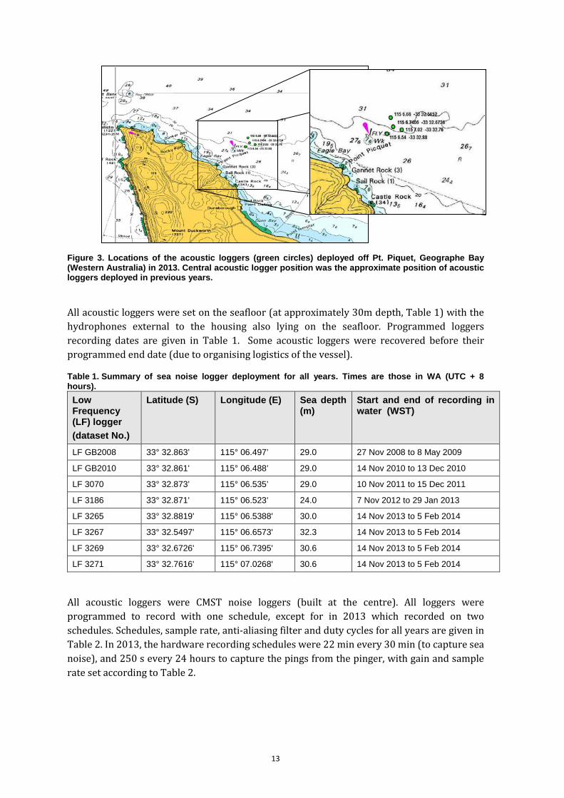
Figure 3. Locations of the acoustic loggers (green circles) deployed off Pt. Piquet, Geographe Bay (Western Australia) in 2013. Central acoustic logger position was the approximate position of acoustic loggers deployed in previous years.

All acoustic loggers were set on the seafloor (at approximately 30m depth, Table 1) with the hydrophones external to the housing also lying on the seafloor. Programmed loggers recording dates are given in Table 1. Some acoustic loggers were recovered before their programmed end date (due to organising logistics of the vessel).

Table 1. Summary of sea noise logger deployment for all years. Times are those in WA (UTC + 8 hours). Low Frequency (LF) logger (dataset No.)

Latitude (S) Longitude (E) Sea depth (m)

Start and end of recording in water (WST)

LF GB2008 33° 32.863’ 115° 06.497’ 29.0 27 Nov 2008 to 8 May 2009

LF GB2010 33° 32.861’ 115° 06.488’ 29.0 14 Nov 2010 to 13 Dec 2010

LF 3070 33° 32.873’ 115° 06.535’ 29.0 10 Nov 2011 to 15 Dec 2011

LF 3186 33° 32.871’ 115° 06.523’ 24.0 7 Nov 2012 to 29 Jan 2013

LF 3265 33° 32.8819' 115° 06.5388' 30.0 14 Nov 2013 to 5 Feb 2014

LF 3267 33° 32.5497' 115° 06.6573' 32.3 14 Nov 2013 to 5 Feb 2014

LF 3269 33° 32.6726' 115° 06.7395' 30.6 14 Nov 2013 to 5 Feb 2014

LF 3271 33° 32.7616' 115° 07.0268' 30.6 14 Nov 2013 to 5 Feb 2014

All acoustic loggers were CMST noise loggers (built at the centre). All loggers were programmed to record with one schedule, except for in 2013 which recorded on two schedules. Schedules, sample rate, anti-aliasing filter and duty cycles for all years are given in Table 2. In 2013, the hardware recording schedules were 22 min every 30 min (to capture sea noise), and 250 s every 24 hours to capture the pings from the pinger, with gain and sample rate set according to Table 2.

14

Table 2. Noise logger settings and sampling regimes for all years of recording. Deployment year

Schedule Total gain (dB)

Sample rate / anti-aliasing filter (kHz)

Duty cycle

2008-2009 Schedule 1 40 6/2.8 200 s every 900 s

2010 Schedule 1 40 12/5 800 s every 900 s



2013 Schedule 1 40 4 / 1.8 1380 s every 1800 s

2013 Schedule 2 (to capture Pinger)

40 20 / 9 25 s every 86400 s

The frequency response of all four noise loggers in ADC units per 1 µPa was calibrated before deployment and will be after recovery by inputting white noise of known level in series with the hydrophone and then correcting the recorded signal for the hydrophone sensitivity. The hydrophone signal was amplified using an impedance matching pre-amplifier of 20 dB gain and a channel amplifier with gain setting of 20 dB. Signals were high-pass filtered with a roll-off starting at 8 Hz so as to reduce the naturally high levels of low frequency sea noise and hence increase the dynamic range of the recording system. The amplified signals were low-pass filtered by an anti-aliasing filter and then fed to a 16-bit analogue-to-digital converter (ADC). Sampling rates and anti-aliasing filter settings are given in Table 2.

Land-based theodolite survey observations A land-based theodolite station was positioned at 51 meters above sea level at Pt. Piquet (‘Hill 50’ in Meelup Regional Park) to provide daily observations of habitat use, distribution, and behaviour of whales near-shore during all survey years. This platform allowed the collection of positional and behavioural information without disturbance to the whales by the observers. Main observation techniques include: 1) scan sampling to obtain relative abundance estimates, distribution (since the theodolite allows for obtaining accurate positions of the whales), group composition and size, and information about general local movements, direction and path of travel; and 2) focal follow sampling to describe locations, habitat use, orientations, speeds, surfacing-respiration-dive parameters, and other surface-visible behaviours (aggressive and non-aggressive) as a response to vessel traffic and approaches. In addition, tracking of the position and speed of vessels in the study area were done with the theodolite, including the whale watch vessels.

For land-based observations, all whales, other marine mammals, and vessels detected within a 10 km radius were recorded. All observations were conducted by teams of three to four observers, one to two dedicated to scanning up to the horizon, one dedicated to theodolite tracking, and the fourth dedicated to operating a computer linked to the theodolite and running Vadar (Visual Detection and Ranging at sea) software (E. Kniest, 2011; Figure 4 and Figure 5). Vadar has been designed for tracking whale and vessel movements and whale behaviour in real time as they pass through the study area (Figure 5). The target period for visual observations at the tracking station was of 6-8 hours a day, but varied depending upon weather conditions. Teams undertook observations in conditions of less than Beaufort 3 and

15

on the lower scale of Beaufort 4 (with the exception of a few hours where they operated on the low end of Beaufort 5). High Beaufort conditions introduced error in sightings due to white caps and white horses and observer fatigue. Teams rotated at mid-day to minimize fatigue. The first shift commenced at 7:30am and finished approximately at 11:00 to avoid the midday heat. Afternoon shifts commenced at 14:00 and finished at 17:45.

Figure 4. Land-based hill observation team. Depicted in the photos are: (A) two spotters and the theodolite operator, and (B) a spotter, the theodolite operator and the computer operator running Vadar software.

16

Figure 5. Example of whale, vessel, and dolphin observations and tracks displayed in real time in Vadar over a ~4 hour period on the 21 November 2013 (pods are labelled with letters and have a blow or breach icon, and vessels are labelled with numbers).

17

The study area was scanned continuously for sighting cues of whales, other marine fauna and vessels. When a sighting was made, the spotters measured the bearing and reticules from the horizon using reticule binoculars and reported these and the sighting cue, pod composition and species to the VADAR operator. The spotter directed the theodolite operator to locate the group so that more accurate positions could be recorded using the theodolite. Under ‘scan mode’, using spotter binoculars and the theodolite, groups of whales, other marine mammals, and vessels were tracked (positions, sighting cue, and group composition recorded) within the study area when they were within detectability. When there was a single group in the study area and the group was within 5 km range of the land-based observation station or when there was vessel interaction, a shift to ‘focal follow’ mode was made, and the theodolite operator tracked all surfacings and behaviours and attributed them to individuals within the group where possible. The spotter continued to scan the entire area for arrivals of new groups. Focal follows allowed for the collection of detailed information on group behaviour and vessel interactions. Data was analysed with the software R (V3.02) using RStudio (R Core Team, 2013).

Vessel survey observations Vessel work using a 5m Zodiac with 70hp engine were conducted during Beaufort sea states of 3 or less. Vessel-based visual surveys were only conducted in 2013, and followed pre-determined transects designed to provide equal effort across the southerly whale transit route of Geographe Bay. These data will complement the land-based visual observations to provide information on abundance, distribution, group size and environmental correlates of whales within Geographe Bay. Transects were designed to overlap with land-based surveys. Furthermore the boat-based surveys are the only means for providing information on photo-identification which provides information on connectivity, movements and site fidelity of widely spaced habitats such as the Perth Canyon and the Bonney Upwelling region.

Observations of all marine fauna were recorded by two observers on the vessel continuously scanning 180 degree of the ocean from the bow to stern; one on the port and the other on the starboard side Figure 6). The vessel transited transects at a velocity 10-12 knots.

Figure 6. Diagram showing observer placement on vessel during surveys.

Observer 1 viewing 180 degrees from bow to stern of port side

Observer 2 viewing 180 degrees from bow to stern of starboard side

18

Observer 1 working on the port side used a DSLR Pentax K30 camera fitted with a GPS accessory compass capability, and a 100-300 telephoto lens to collect bearing and allow for distance measurements by photographing the horizon. Calculations of distance were made using algorithms that use distances down from the horizon where the sightings were made in the equations. Observer 1 needed to be immediately ready to photograph to capture the first surfacing of the groups. This enables estimation of the detection function (with range from the vessel). Observer 2 on the starboard side steered the vessel on the track and recorded sighting data (cue, species, pod composition, time, position and date) and environmental data (wind direction and speed, cloud cover and water depth and temperature) onto a log sheet.

Line transect surveys were designed in Distance (6.0) to maximise equal probability of coverage effort over the study area. The surveys were then plotted in ArcGIS and vertices positions input into a hand-held GPS for use on the vessel. The survey consisted of 4 parallel lines running SE to NW along Cape Naturaliste adequately covering the general southward movement of migrating whales. The direction of transect coverage (from south west to northeast) and velocity of the vessel were selected to minimise the probability of double counting (Figure 7). The total distance over all transects was approximately 60km and were spaced 4 km apart (a half strip width of 2 km). The total study area was covered over a projected period of 3 - 4 hours of observation. This design allowed for time to break temporarily from transects when sightings were made to collect photo-identification information.

Figure 7. (A) Study area (shaded in red) with transects design (using Distance 6.0 and ArcGIS 10.0) to provide optimal transect travel time and coverage (~2km half strip width). (B) Transect lines plotted for inputting into vessel GPS.

19

3. Results 3.1. Abundance of baleen whales over the peak of the blue whale migration period Relative Abundance from Land-based Surveys Land-based visual observations effort ranged from 124.75 hours during 28 survey days over a 38 day field season in 2010 to 57.2 hours during 13 survey days over a 18 day field season in 2011, 24 days over a 28 day field season in 2012, and 13 days over a 14 day field season in 2013 (effort for all years is presented in Table 3). During the survey days, the hours of observation was weather dependent, and varied among years.

Table 3. Summary of land-based hill observation effort. Year Field dates

Number of days of surveys (of total

days in the survey period)

Number of hours of survey (hrs)

2010 4 Nov to 6 Dec 28 (35) 124.8

2011 13 Nov to 29 Nov 13 (18) 57.2

2012 5 Nov to 2 Dec 24 (28) 103.2

2013 15 Nov to 28 Nov 13 (14) 57.9

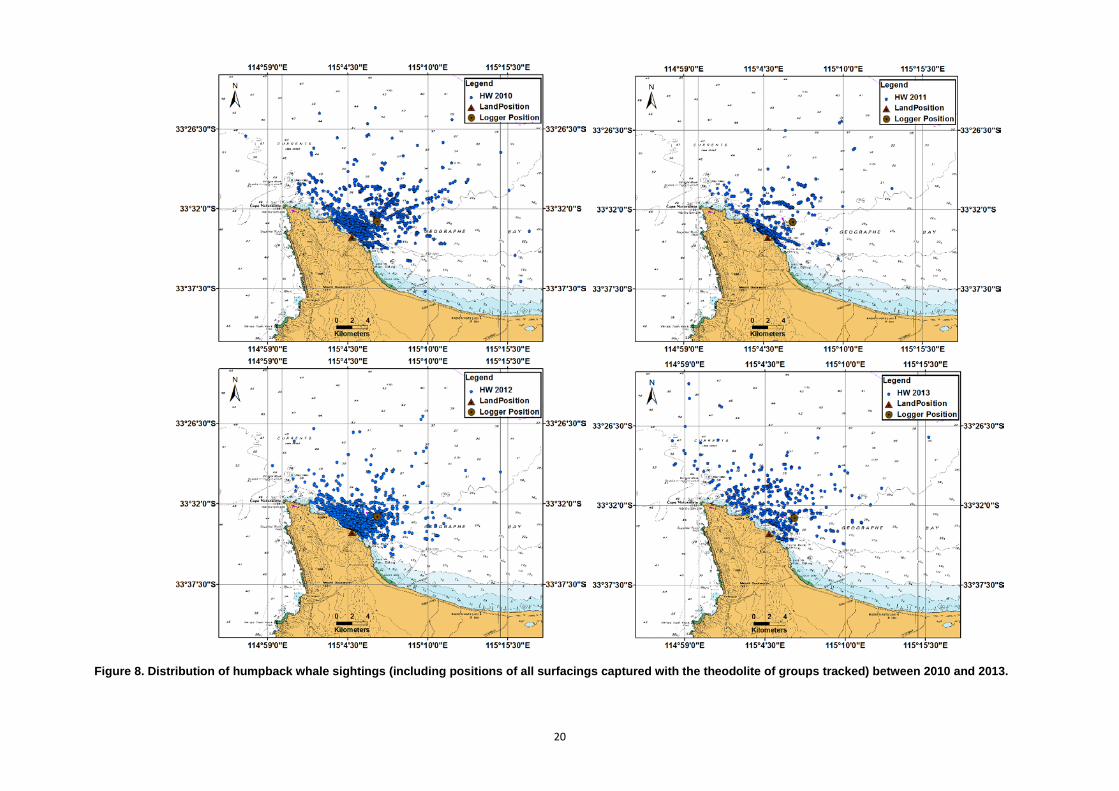
The total number of whales observed during the four years of land-based field surveys was 2061 in 1142 groups. Of these, 1952 whales (in 1077 groups) were humpbacks and 109 (in 65 groups) were blue whales. No southern right whales were sighted during land-based surveys, although these are regularly reported during the month of August and September, and occasionally during October. The total number of whales observed and distribution of the sightings varied among years, which was influenced by survey effort (Figure 8, Figure 9). One minke whale group composed of a mother and calf was sighted in 2010 (November 24th). Humpback whales were observed from the land-based observation platform as far as the detection range allowed indicating that they use the entire range within detection, and certainly use that outside the range of detection. Blue whales were detected closer to the Pt. Piquet, tracking the coast from a south-easterly to a north-westerly direction. The detection range was much smaller than for humpback whales, but this is likely due to more subtle surface behaviours than those of humpback whales. Blue whales do not breach or slap their pectoral fins on the surface of the water.

20

Figure 8. Distribution of humpback whale sightings (including positions of all surfacings captured with the theodolite of groups tracked) between 2010 and 2013.

21

Figure 9. Distribution of blue whale sightings (including positions of all surfacings captured with the theodolite of groups tracked) between 2010 and 2013.

22

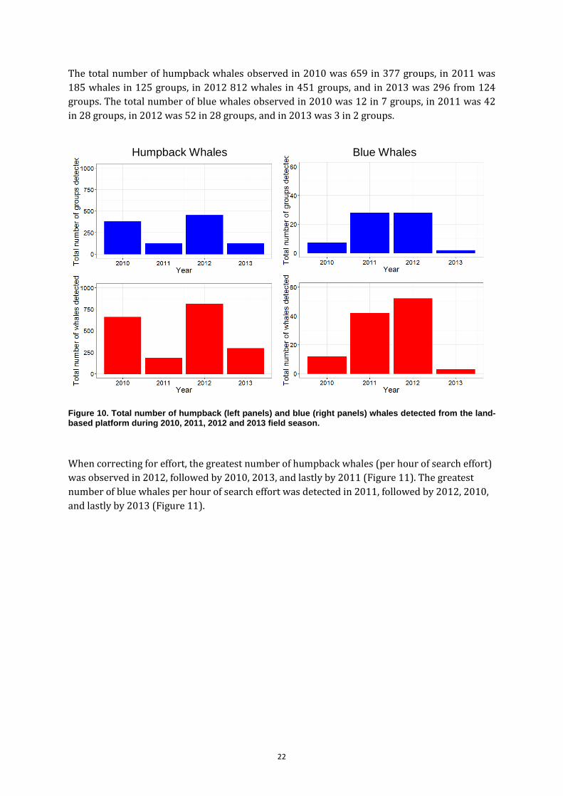
The total number of humpback whales observed in 2010 was 659 in 377 groups, in 2011 was 185 whales in 125 groups, in 2012 812 whales in 451 groups, and in 2013 was 296 from 124 groups. The total number of blue whales observed in 2010 was 12 in 7 groups, in 2011 was 42 in 28 groups, in 2012 was 52 in 28 groups, and in 2013 was 3 in 2 groups.

Figure 10. Total number of humpback (left panels) and blue (right panels) whales detected from the land-based platform during 2010, 2011, 2012 and 2013 field season.

When correcting for effort, the greatest number of humpback whales (per hour of search effort) was observed in 2012, followed by 2010, 2013, and lastly by 2011 (Figure 11). The greatest number of blue whales per hour of search effort was detected in 2011, followed by 2012, 2010, and lastly by 2013 (Figure 11).

Humpback Whales Blue Whales

23

Figure 11. Average number of humpback (left panels) and blue (right panels) whales detected per hour from the land-based platform during 2010, 2011, 2012 and 2013 field season.

The numbers of whales per hour detected over the survey dates also varied over the years (Figure 12). In 2010, the number of humpback whales detected per hour dropped from the first survey day in early November to the last survey day in early December. This drop in overall numbers per hour of effort searching was consistently seen over all years. In 2010, there was a rise and drop in numbers per hour detected around the third week of November. This same peak appeared to occur in 2012 and 2013. In 2011 a number of survey days around this period were missed due to bad weather.

For blue whales, a peak in numbers per hour of search effort was evident in 2011 and 2012 from around the 7th to the 29th of November. In contrast, very low numbers were observed in 2010 and 2013 during this period (Figure 12).


24

Figure 12. Average number of humpback (left panels) and blue (right panels) whales detected per hour from the land-based platform over the survey field seasons during 2010, 2011, 2012 and 2013.


25

Absolute Abundance from Land-based Surveys

Non-parametric spline interpolation was used to estimate counts on days when surveys were not able to be conducted due to poor weather. The smoothing parameter (λ) was selected based on a performance criteria of the model which minimises the expected error. This was done by using Generalized Cross Validation (GCV). The model was fit to the average number of whales observed per hour multiplied by the number of hours in a day (24). The number of whales expected per day on survey days plus those estimated with the non-parametric model on non-survey days over the field season gave the total estimated whales that would have been observed during the field season if surveys could have been done continuously day and night and on bad weather days (Figure 13 and Figure 14). These estimates do not correct for detectability of the animals - that is, the number of whales that were not available to be detected (moved through the study area for a brief period of time without surfacing) and those available but were not detected (due to lower visibility at larger ranges or perception bias). Therefore the estimates here are conservative in that a greater number of whales would have been estimated if detectability were included in the estimation process. A detection curve with number of animals detected as a function of range for correcting for those not detected was not undertaken since this would assume that the distribution is homogenous over the study area. Vessel surveys were trialled in 2013 with the intent of implementing these with greater effort in future surveys to provide distributional information so that a correction for detectability can be made.

26

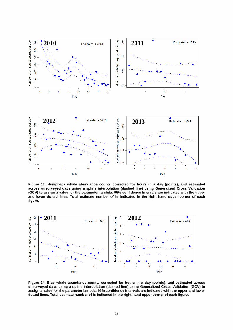
Figure 13. Humpback whale abundance counts corrected for hours in a day (points), and estimated across unsurveyed days using a spline interpolation (dashed line) using Generalized Cross Validation (GCV) to assign a value for the parameter lambda. 95% confidence Intervals are indicated with the upper and lower dotted lines. Total estimate number of is indicated in the right hand upper corner of each figure.

Figure 14. Blue whale abundance counts corrected for hours in a day (points), and estimated across unsurveyed days using a spline interpolation (dashed line) using Generalized Cross Validation (GCV) to assign a value for the parameter lambda. 95% confidence Intervals are indicated with the upper and lower dotted lines. Total estimate number of is indicated in the right hand upper corner of each figure.

2010 2011

2012 2013

2011 2012

27

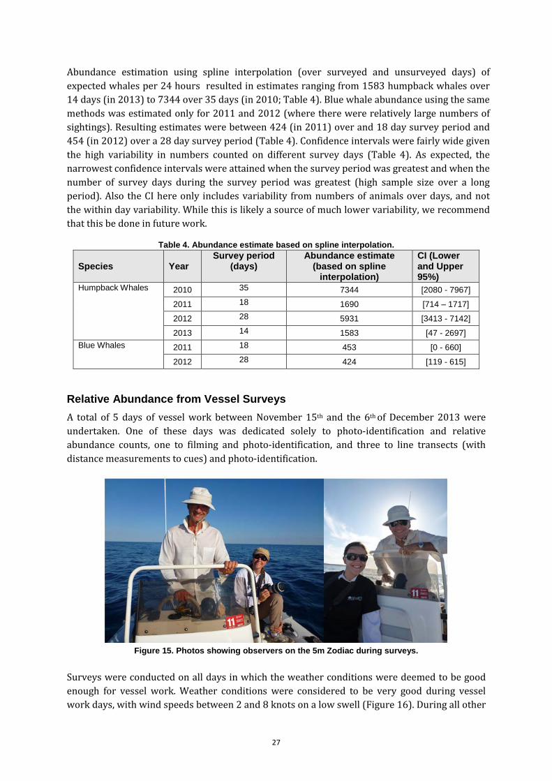
Abundance estimation using spline interpolation (over surveyed and unsurveyed days) of expected whales per 24 hours resulted in estimates ranging from 1583 humpback whales over 14 days (in 2013) to 7344 over 35 days (in 2010; Table 4). Blue whale abundance using the same methods was estimated only for 2011 and 2012 (where there were relatively large numbers of sightings). Resulting estimates were between 424 (in 2011) over and 18 day survey period and 454 (in 2012) over a 28 day survey period (Table 4). Confidence intervals were fairly wide given the high variability in numbers counted on different survey days (Table 4). As expected, the narrowest confidence intervals were attained when the survey period was greatest and when the number of survey days during the survey period was greatest (high sample size over a long period). Also the CI here only includes variability from numbers of animals over days, and not the within day variability. While this is likely a source of much lower variability, we recommend that this be done in future work.

Table 4. Abundance estimate based on spline interpolation.

Species Year Survey period

(days) Abundance estimate

(based on spline interpolation)

CI (Lower and Upper 95%)

Humpback Whales 2010 35 7344 [2080 - 7967]

2011 18 1690 [714 – 1717]

2012 28 5931 [3413 - 7142]

2013 14 1583 [47 - 2697] Blue Whales 2011 18 453 [0 - 660]

2012 28 424 [119 - 615] Relative Abundance from Vessel Surveys A total of 5 days of vessel work between November 15th and the 6th of December 2013 were undertaken. One of these days was dedicated solely to photo-identification and relative abundance counts, one to filming and photo-identification, and three to line transects (with distance measurements to cues) and photo-identification.

Figure 15. Photos showing observers on the 5m Zodiac during surveys.

Surveys were conducted on all days in which the weather conditions were deemed to be good enough for vessel work. Weather conditions were considered to be very good during vessel work days, with wind speeds between 2 and 8 knots on a low swell (Figure 16). During all other

28

days, weather conditions ranged from 14 to 18 knots. Line transect surveys conducted on good weather days covered a total distance of 165km over 13 hours observation effort (Table 5).

Figure 16. Plot of weather conditions during main field work period and during vessel surveys. Bars in blue and red are based in data collected from two weather stations close to the study area (daily average), bars in green are qualitative wind speed estimations made from the vessel. Wind speeds (mean knots) for each of the 5 surveys.

The survey transects effectively overlapped the study area covered by the land-based platform (Figure 17). As a trial for future double platform work where the distribution of whales recorded by the vessel survey can be used to correct for detectability as a function of range for land-based observations, the survey design was found to be effective.

29

Figure 17. Map showing coverage of vessel surveys in relation to land-based observations in 2013, using the vessel survey track (dark blue circles) from the 16th of November 2013 as an example of a typical track overlayed by land-based observations of surfacing groups of whales (light blue circles).

Over the small number of vessel trial days a relatively high number of marine mega-fauna were sighted, with humpback whales being the most abundant of these (despite the survey period being outside of the peak humpback whale migration period; Table 5 and Table 6). Several blue whale sightings were also made, despite significantly lower overall numbers of blue whales during the two week survey period than in 2011 and 2012.

30

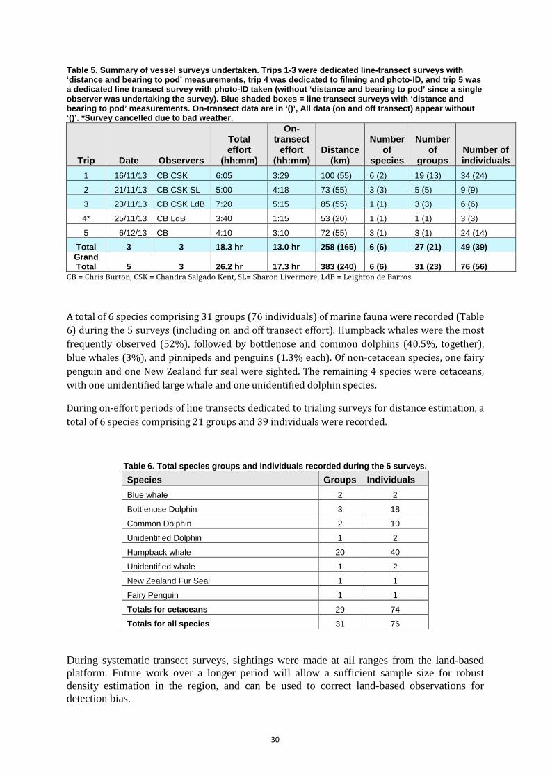
Table 5. Summary of vessel surveys undertaken. Trips 1-3 were dedicated line-transect surveys with ‘distance and bearing to pod’ measurements, trip 4 was dedicated to filming and photo-ID, and trip 5 was a dedicated line transect survey with photo-ID taken (without ‘distance and bearing to pod’ since a single observer was undertaking the survey). Blue shaded boxes = line transect surveys with ‘distance and bearing to pod’ measurements. On-transect data are in ‘()’, All data (on and off transect) appear without ‘()’. *Survey cancelled due to bad weather.

Trip Date Observers

Total effort

(hh:mm)

On-transect

effort (hh:mm)

Distance (km)

Number of

species

Number of

groups Number of individuals

1 16/11/13 CB CSK 6:05 3:29 100 (55) 6 (2) 19 (13) 34 (24)

2 21/11/13 CB CSK SL 5:00 4:18 73 (55) 3 (3) 5 (5) 9 (9)

3 23/11/13 CB CSK LdB 7:20 5:15 85 (55) 1 (1) 3 (3) 6 (6)

4* 25/11/13 CB LdB 3:40 1:15 53 (20) 1 (1) 1 (1) 3 (3)

5 6/12/13 CB 4:10 3:10 72 (55) 3 (1) 3 (1) 24 (14) Total 3 3 18.3 hr 13.0 hr 258 (165) 6 (6) 27 (21) 49 (39)

Grand Total 5 3 26.2 hr 17.3 hr 383 (240) 6 (6) 31 (23) 76 (56)

CB = Chris Burton, CSK = Chandra Salgado Kent, SL= Sharon Livermore, LdB = Leighton de Barros

A total of 6 species comprising 31 groups (76 individuals) of marine fauna were recorded (Table 6) during the 5 surveys (including on and off transect effort). Humpback whales were the most frequently observed (52%), followed by bottlenose and common dolphins (40.5%, together), blue whales (3%), and pinnipeds and penguins (1.3% each). Of non-cetacean species, one fairy penguin and one New Zealand fur seal were sighted. The remaining 4 species were cetaceans, with one unidentified large whale and one unidentified dolphin species.

During on-effort periods of line transects dedicated to trialing surveys for distance estimation, a total of 6 species comprising 21 groups and 39 individuals were recorded.

Table 6. Total species groups and individuals recorded during the 5 surveys. Species Groups Individuals Blue whale 2 2

Bottlenose Dolphin 3 18

Common Dolphin 2 10

Unidentified Dolphin 1 2

Humpback whale 20 40

Unidentified whale 1 2

New Zealand Fur Seal 1 1

Fairy Penguin 1 1

Totals for cetaceans 29 74 Totals for all species 31 76

During systematic transect surveys, sightings were made at all ranges from the land-based platform. Future work over a longer period will allow a sufficient sample size for robust density estimation in the region, and can be used to correct land-based observations for detection bias.

31

Figure 18. Example of boat tracks (dark blue) overlayed by positions at first detection of animals on a single survey day (16th of November 2013). Positions were calculated from the distance down from the horizon to the animals using photographs. Cues were recorded as part of the trial since these are used for correcting biases in detection due to some cues being more easily detected than others. Of the cues (the first behaviour observed which was the ‘cue’ to the sighting) during line transect surveys with distance measurements, ‘body’ (where a part of the body was observed) and ‘blow’ represented 56% and 33% of the total cues, respectively (Figure 19). Blue and unidentified large whales sighting cues were ‘blow’ only, while humpback whales were sighted with both ‘blow’ and ‘body’ cues. All dolphins were sighted by a ‘body’ cue.

32

Figure 19. Percentages of sighting cues.

Of the 29 groups of cetaceans, ~15 humpback and 2 blue whales (Figure 20) were photo-identified during the surveys. Both blue whales were checked with the WWR blue whale photo-id database (updated recently to include dates from 1994 to 2010), and no matches were recorded. Further database updates to the catalogue are required to compare photos to those taken during 2011-2013 (this work is currently outside of the scope of this project).

Figure 20. (A) Blue whale left dorsal (LD) photo taken during Trip 12, and (B) blue whale LD photo taken during Trip 13.

33

3.2. Changes in the soundscape environment during the peak of the blue whale migration

During the first year of acoustic surveys, recordings were made over approximately a five month period from the 27th of November 2008 to the 8th of May 2009. In 2010 recordings were made only over the peak period of the blue whale migration in Geographe Bay, from the 14th of November to the 13th of December. Peak periods for humpback whales and blue whales were estimated based on data previously collected by volunteers from Western for Whale Research and Dunsborough Coast and Land Care Community group at Pt. Piquet (Burton abd Glencross 2014, Pers. comm.). Similarly, recordings in 2011 were made only over the peak period of blue whale migration, from the 13th of November to the 15th of December. In 2012 recordings were made over a slightly longer period, from the 7th of November to the 21th of December, and in 2013 from the 14th of November 2013 to the 29th of January 2014. Here we presents results from November and December for each year – data coinciding with the peak of the blue whale migration period.

Spectrograms from recordings in 2008 are presented in Figure 22 and Figure 23, from 2010 in Figure 24 and Figure 25, in 2011 in Figure 26 and Figure 27, from 2012 in Figure 28, Figure 29, and Figure 30, and 2013 in Figure 31, Figure 32, Figure 33, and Figure 34.

Ambient and anthropogenic noise sources Ambient noise in Geographe Bay typically ranged from 65-75 dB re 1 µPa2 Hz-1 in the absence of vessels to 110 dB re 1 µPa2 Hz-1 when vessels were near the noise logger. Physical noise was dominated by wave and wind activity which also often had a diurnal pattern (Figure 25), reflecting the pattern of the incoming, afternoon seabreeze. Intense periods occurred early in December in all years, and during other periods as weather fronts moved in (i.e. mid December in 2013). Physical noise driven by wind or breaking waves generated differences in the power spectrum density of ambient noise. These differences are shown in Figure 21 during two different time periods of 6 hours during one typical day in December in 2008 (at night between 11pm and 5am and in the afternoon between 12am and 8pm). It is clear that the afternoon breeze forcing wind waves increases the noise level noticeably over the entire frequency range between 10 Hz to 3 kHz. The increase is more significant at frequencies greater than 50 Hz.

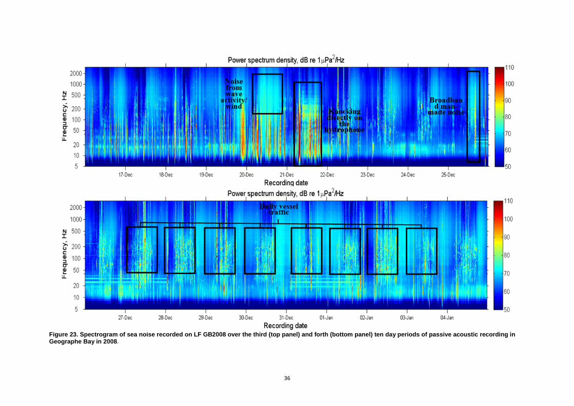
Underwater noise from anthropogenic sources over all years was dominated by vessels primarily fishing and recreational vessels. Vessel noise was most frequent and intense during December in all years, and in particular between mid-December and the Christmas holidays which is evident in recordings that extended to these dates in 2008 and 2013. Diurnal (day/night) patterns were evident during these intense periods, with the most frequent vessel noise often around midday. An example of this intense diurnal pattern is shown in the ten-day spectrogram beginning on the 26th of December 2008 (bottom panel of Figure 23). Vessel noise changed the noise environment substantially in the area, adding more than 20 dB to the ambient noise. This occurred on most days, with particularly large contributions on weekends during good weather periods.

34

Other sources of low frequency man-made noise was detected in the sea noise at times. Sources were identified using a Power Spectrum Density (PSD) analysis. PSD is the power expressed in spectral level units (dB re 1 µPa per Hz). The value is normalised so that the intensity is presented in the equivalent of a 1-Hz bandwidth. These units are used widely in underwater acoustics and are useful for comparing the energy content of different sources as the units can be directly overlain, even if, for example, the power spectral frequency resolution differs.

Here, low-frequency noise was evident in late December in 2008 and had a maximum PSD of more than 100 dB at frequencies between 20 Hz and 40 Hz. This level is much higher than the regular noise level at those frequencies, even for the busiest vessel traffic period.

Figure 21. Power spectrum density of ambient noise averaged over 6-hour periods between 12 am and 12 pm of no wind (blue), high wind (green), and the maximum vessel noise (red) during one day in December 2008. The dotted lines show the standard deviation of fluctuations at different frequencies. Biological noise sources Underwater noise from biological sources recorded during the peak of the blue whale migration (during November and December) in all years in which recordings were made (2008, 2010, 2011, 2012, and 2013) were dominated by baleen whales, fish and snapping shrimp (Figure 22 to Figure 34). Blue and humpback whale vocalisations dominated the biological sounds (examples are given in Figure 22, Figure 23, Figure 24, Figure 25, Figure 26, Figure 28, and Figure 31). Blue whale vocalisations are lower in frequency than the most humpback whale vocalisations (see example of non-song sounds in Figure 28 and Figure 31), and can be distinguished by their steriotypical calls (Gavrilov et al., 2012) as well as their non-song sounds (Recalde-Salas et al., 2014).

35

.

Figure 22. Spectrogram of sea noise recorded on LF GB2008 over the first (top panel) and second (bottom panel) ten day periods of passive acoustic recording in Geographe Bay in 2008.

Vessels

36

Figure 23. Spectrogram of sea noise recorded on LF GB2008 over the third (top panel) and forth (bottom panel) ten day periods of passive acoustic recording in Geographe Bay in 2008.

37

Figure 24. Spectrogram of sea noise recorded on LF GB2010 over the first (top panel) and second (bottom panel) ten day periods of passive acoustic recording in Geographe Bay in 2010.

38

Figure 25. Spectrogram of sea noise recorded on LF GB2010 over the last eleven day period of passive acoustic recording in Geographe Bay in 2010.

39

Figure 26. Spectrogram of sea noise recorded on LF 3070 over the first ten day period (top panel) of passive acoustic recording, and spectrogram (bottom, left panel) and waveform (bottom, right panel) of blue whale song recorded on the 17th of November 2011 at 09:05 in Geographe Bay.

40

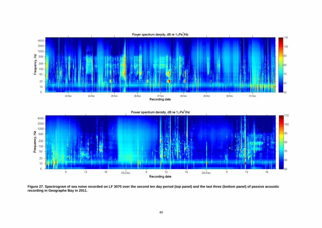
Figure 27. Spectrogram of sea noise recorded on LF 3070 over the second ten day period (top panel) and the last three (bottom panel) of passive acoustic recording in Geographe Bay in 2011.

41

Figure 28. Spectrogram of sea noise recorded on LF 3186 over the first ten day period (top panel) of passive acoustic recording in Geographe Bay in 2012; spectrogram (left, middle panel) and waveform (right, middle panel) of blue whale non-song sounds produced on the 9th of November 2012 at 20:37; high time-resolution spectrograms of two of the non-song sounds from the middle panels (bottom panels).

42

Figure 29. Spectrogram of sea noise recorded on LF 3186 over the second (top panel) and third (bottom panel) ten day periods of passive acoustic recording in Geographe Bay in 2012.

43

Figure 30. Spectrogram of sea noise recorded on LF 3186 over the last ten day period of passive acoustic recording in Geographe Bay in 2012 (recordings after the 22nd are in air after recovery of the acoustic logger).

44

Figure 31. Spectrogram of sea noise recorded on LF 3269 over the first ten day period (top panel) of passive acoustic recording in Geographe Bay in 2013, and spectrogram (left, bottom panel) and waveform (right, bottom panel) of example of multiple humpback whale songs produced simultaneiously on the 19th of November at 15:00.

45

Figure 32. Spectrogram (left panel) and waveform (right panel) of a recreational vessel recorded on the 20th of November 2013 at 15:00 in Geographe Bay.

46

Figure 33. Spectrogram of sea noise recorded on LF 3269 over the second (top panel) and third (bottom panel) ten-day periods of passive acoustic recording in Geographe Bay in 2013.

47

Figure 34. Spectrogram of sea noise recorded on LF 3269 over the last ten-day periods of passive acoustic recording in Geographe Bay in 2013.

48

Humpback whale song was most intense in early to mid-November during all years (with multiple singers singing simultaneiously). Humpback whale song dropped off dramatically between late November and early December.

Since blue whales were the focus of this study, counts were made of vocalising blue whales by counting acoustic cues. Counts were made with the assumption that blue whales travel through the study area and outside of acoustic detection within an hour. Multiple non-overlapping signals attributed to blue whales were assumed to be from a single animal. This assumption was based on observations of blue whale groups tracked with the theodolite through the study area (multiple groups within the study area were extremely rare (occurring once in the four years of theodolite tracking) and the time taken for them to traverse the acoustic range (estimated in Salgado Kent et al 2012) was less than an hour. The number of blue whales detected during the recording period varied over the years of recording with overall numbers greatest in 2011 (an estimated 56 individuals were detected vocalising in 2011, 24 in 2012, and 13 in 2013, Figure 35). The peak in number of vocalisations per hour also varied over years, in that there was a clear peak in mid to late November in 2011, but this was less marked or absent in 2010, 2012, and 2013 (Figure 35).

Blue whale acoustic cues can be directly compared to land-based survey counts in future work to estimate detection bias to further develop acoustic abundance estimation

Figure 35. Number of blue whales detected vocalising per day (in 2011, 2012, and 2013).

Night time fish choruses were also evident (example over the ten-day spectrogram in Figure 25), and snapping shrimp occurred in all recordings. Fish choruses were most clearly distinguished in November and December 2008.

49

3.3. Disturbance during the peak of the blue whale season Because blue whales were the focus of this study, disturbance from vessel interactions with blue whales was quantified. While vessel interactions occurred at varying distances, those occurring within recommended slow or no approach zones by the Australian whale-watching regulations were quantified. Australian whale-watching regulations recommend that within 300m of whales vessels must use caution and travel at low speed, and a zone of 100m is a “no approach” zone without a permit (Australian Government, 2005). Based on these recommendations, vessel interactions within 300m of blue whales were quantified.

The land-based theodolite surveys were used to extract distances of vessels to whale groups. Whale group composition, behaviour and surfacing locations were recorded and mapped in real-time in Cyclops, and vessel type, activity and movements were also recorded.

During the months of November-December between 2010 and 2013, 50 pygmy blue whale groups (92 individuals) were tracked during 341.9 hours of observation. 50% were involved in at least one vessel interaction. This amounted to 25 groups being involved in 36 whale-vessel interactions (since some involved multiple vessels interacting with a single whale group). The 36 recorded whale-vessel interactions involved 58% recreational, 32% research, and 10% tourism boats.

The proportion of vessel interactions varied among group composition with cow-calf pairs (MC) having the most vessel interactions (9 groups out of 12) whilst multiple adult groups had the least (7 groups out of 17; Figure 36).

Figure 36. The percentage of blue whale groups of different group composition types observed during land-based observations in Geographe Bay (blue bars) during 2010, 2011, 2012, and 2013, and the percentage in each group composition category involved in one or more vessel interactions (red bars). Of the 25 groups involved in vessel interactions, 9 groups were involved in multiple vessels interacting with them during their use of the bay (Figure 37).

50

Figure 37. The number of pygmy blue whale groups involved in no interactions (0), interactions with one vessel (1), with two vessels (2), and with three vessels (3) during their use of Geographe Bay during land-based observations in 2010, 2011, 2012, and 2013.

4. Discussion and Conclusions 4.1. Abundance Estimations The numbers of whales using the resting and migratory study area within Geographe Bay on their journey south to feeding grounds during the peak of the blue whale migration revealed high variability among years and within survey periods. Humpback whales observed per hour fluctuated from day to day, which corresponds to known ‘pulses’ in the migration of this species. There was a consistent trend of decreasing numbers of humpback whales towards December among all years (2010-2013) coinciding with the end of the humpback whale migration through the study area. No consistent peak in numbers was detected in humpback whale numbers during the survey periods across years. This is likely because the peak occurs during September and October (WWR and D-CALC unpublished community-collected 9-year data set). Right whales were not observed during the survey period, however they were present in Geographe Bay in the leading up to the survey period (WWR and D-CALC unpublished community-collected 9-year data set; Ian Wiese pers. comm.). Minke whales were seen on one occasion.

Based on 19th and 20th century whaling data (Glencross and Burton, 2012 – reference to Seymour diaries) minke whales have historically been sighted in Geographe Bay, although in fewer numbers than humpback and blue whales. Blue whales observed per hour varied dramatically among survey periods in different years. While the peak in blue whales occurred in mid to late November in 2011 and 2012, the peak in 2013 occurred earlier (before the survey period had begun; WWR and D-CALC unpublished community-collected 9-year data set). Because of the variability in the peaks and the different timing of the peaks of the different species, a longer survey period over several years is required to more accurately define this variability, and relate this to changes in the environment.

51

Estimates of abundance of whales passing through the study area over the entire survey period, including during day and night time hours (24 hours) and during non-survey, bad-weather days revealed variable estimates due to the length of the survey period as well as the variability in numbers of whales moving through the area. Based on the last estimates of the population size of Breeding Group D humpback whales (which migrate along the west coast of Australia) in 2008 of approximately 33,000 (33,333 estimated by Salgado Kent et al., 2012 and 33,850 estimated by Hedley et al. 2011), we can obtain a rough idea of the minimum proportion of the population that can move through Geographe Bay in a season during the period surveyed. If the population has not plateaued, and increase rates of 10% per annum (Salgado Kent et al., 2012) are still reasonable, then the current population would be expected to be over 50,000 animals. A rough estimate would be that greater than 12% (greater, since detectability was not incorporated in the estimate) of 50,000 animals can move through the study area in the November/early December period. Since November is not the peak month for humpback whales in the area, and the migration of humpbacks through Geographe Bay occurs over a period longer than 3 months, a significantly larger proportion would be expected to use the bay during the entire southern migration period. To estimate the proportion over the entire migration season, a full-season study would need to be conducted.

For blue whales, the only abundance estimates currently available for the east Indian Ocean population that have been undertaken are from un-published photo-ID work and from acoustic measurements in 2004 in the Perth Canyon off the coast of Western Australia (McCauley & Jenner, 2010). Both estimates are reported to be similar (McCauley and Jenner, 2010), with acoustic measurements resulting in a mean of 1,110 animals (with a range between 662 and 1559). This is considered to be a fraction of the total pool of the population. While the main migratory corridors have been mapped out (McCauley and Jenner, 2010), it is not clear what proportion of the whales visit key areas during their migration such as the Perth Canyon, Geographe Bay, and the Bonney Upwelling region. Over the peak of the southern blue whale migration period in Geographe Bay a minimum of just under 50% of the number of animals that have been estimated for the Perth Canyon can visit Geographe Bay in a season. While there is established connectivity between Geographe Bay and the Perth Canyon (from photo-ID comparisons by Burton and Jenner), it is unknown what percentage of animals use both locations in a single season, and how this varies over seasons. Further photo identification is needed collected over many years to establish this. The timing of visitation and numbers within Geographe Bay also varies. To establish the extent of the variability a longer field period is needed conducted over multiple years.

For the relative and absolute abundance estimates presented here, the effect of Beaufort conditions, swell, and glare on the detection of whales was not tested. We recommend that future work test these effects and if they are significant, they should be used as covariates in models estimating abundance. In addition to this, the effect of detection bias as a function of range from the observers, availability of the animals for detection, and perception bias of observers was not incorporated in abundance models here. However, as part of the scope of the work, we tested vessel surveys for future work to include double platform surveys (land and vessel) to measure these biases, and incorporate correction factors into abundance models. The

52

vessel surveys with observers using GPS-fitted cameras (with bearing and GPS position recorded in the metadata) allows for the position of the animals in relation to the vessel to be mapped, and the range at the time of detection to be calculated. The range from the vessel is calculated based on the distance of the animals down from the horizon. This technique will allow future vessel-based density estimates of whale groups in the area with known (correctable) range-dependent detection bias. Density estimates can then be used to correct for land-based detection bias. Vessel surveys also provide an effective means of collecting high quality photos for identification of individual whales to enable connectivity among different key blue whale habitats to be determined.

4.2. Acoustic Analysis The acoustic component of the work allowed for the documentation of the soundscape in Geographe Bay and its change over time. The most marked change was the biological acoustic energy, mainly from vocalising humpback and blue whales migrating through the bay, and the increase in vessel noise during weekends and holidays. During the period of whale migration, humpback and blue whales were the dominant sound source in the recordings. By the end of the season, noise from vessels became the dominant source. These occurred over all years. Further analysis is needed to establish dial patterns for blue and humpback whales.

Further seasonal underwater noise recordings will allow for continued monitoring of change in the sound environment, including increases in the anthropogenic energy from changes in human use of the bay. Current acoustic data can also be further queried to produce more detailed information on anthropogenic (and biological) input into the underwater noise environment. The acoustic component also allowed for a count of blue whales based on acoustic cues. More work is required to develop acoustic detections into absolute abundance estimates, which would provide a powerful tool for long-term monitoring whale abundance in Geographe Bay (and elsewhere). Much of the data presented here (from multiple platforms) can be used to progress the development of this technique.

4.3. Vessel Interactions When quantifying whale-vessel interactions within 300m distance, where vessel noise is expected to be most intense and Australian guidelines suggest either low travel speed or ‘no approach’ zones, a relatively high proportion of interactions was recorded. 50% of blue whale groups had interactions at this close range. Cow-calf pairs had proportionally higher interactions, most likely because they are more visible than singletons or adult pairs since they travel more slowly and tend to be at the surface of the water for longer periods. With almost 60% of interactions being with non-permitted recreational vessels, we highly recommend increased access to guidelines and educational material in the region. This can be in the form of informative and educational signs at all boat ramps and key whale observation areas visited by tourists and recreational users around the bay. Key whale observation areas can be fitted with spotting scopes and general information on behaviour, life history, and population status of the species. The effectiveness of improved access to guidelines should be tested by continued monitoring of these interactions, as well as further assessment of the nature and extent of the changes in behaviour of whales involved in vessel interactions.

53

An important component in assessing the extent of impact is to measure the response of whales to vessels moving at different speeds and changing directions. Research permits for example are given under strict ethical approvals, with requirements to minimise disturbance by approaching whales slowly (not from the back or front of the travel direction of the groups or erratically), and minimising the time of the interaction as much as possible. As a final note, improving community awareness through involving the community in citizen science such as the community research program run by Western Whale Research and Dunsborough Coast and Landcare groups, and collaborating with local businesses and government is key to long-term management and conservation.

Finally, in addition to providing key research findings, the work here focused on increasing awareness through media and educational activities. Media included updates on the SouWEST blog (souwest.org), assisting in the collection of film footage of whales by Sea Dog TV International Pty Ltd for IFAW, and discussing the work and whale conservation on radio, as well as through community and scientific presentations. SouWEST is also on Facebook and Twitter. One peer reviewed scientific publication has also resulted during the short period of the work (Recalde-Salas et al. 2014).

References

Gavrilov, A.N., McCauley, R. D., Salgado Kent, C., Tripovich, J. and Burton, C. 2011. Vocal characteristics of pygmy blue whales and their change over time. J. Acoust. Soc. Am. 130(6), 3651-3660.

Glencross, R.N. & Burton, 2013. Nineteenth century whale population of Geographe Bay compared with that of the early 21st century. Third Biennial South West Marine Conference, Bunker Bay, Western Australia. Hedley, S.L., Bannister, J.L. and Dunlop, R.A. 2011. Abundance estimates of Breeding Stock ‘D’ humpback whales from aerial and land-based surveys off Shark Bay, Western Australia, 2008. J. Cetacean Res. Manage. (special issue 3): 209-21

McCauley, R & Jenner, C. 2010. Migratory patterns and estimated population size of pygmy blue whales (Balaenoptera musculus brevicauda) traversing the Western Australian coast based on passive acoustics. Report to the International Whaling Commission Scientific Committee (SC/62/SH26) 9pp.

R Core Team. 2013. R: A language and environment for statistical computing. R Foundation for Statistical Computing, Vienna, Austria. URL: http://www.R-project.org/.

Recalde-Salas, A., Salgado Kent, C.P., Parsons, M.J.G., Marley, S.A., and McCauley, R.D. 2014. Non-song vocalizations of pygmy blue whales in Geographe Bay, Western Australia. J. Acoust. Soc. Am. 135(5), EL213-EL218.


54

Salgado Kent, C., Jenner, C., Jenner, M., Bouchet, P. and Rexstad, E. 2012. Southern hemisphere Breeding Stock D humpback whale population estimates from North West Cape, Western Australia. J. Cetasean Res. Manage. 12(1): 29-38.

Salgado Kent, C., C.P., Gavrilov, A.N., Recalde-Salas, A., Burton, C.L.K., McCauley, R.D., and Marley, S. 2012. Passive acoustic monitoring of baleen whales in Geographe Bay, Western Australia. Proceedings of Acoustics 2012 (Australian Acoustical Society) – Fremantle.

Seymour, F.W. (no date). Castle Rock diary of Frederick William Seymour. Unpublished manuscript, Battye Library. Microfiche acc. No 2838 A1 & 2.

Thomas, L., S.T. Buckland, E.A. Rexstad, J. L. Laake, S. Strindberg, S. L. Hedley, J. R.B. Bishop, T. A. Marques, and K. P. Burnham. 2010. Distance software: design and analysis of distance sampling surveys for estimating population size. Journal of Applied Ecology 47: 5-14. DOI: 10.1111/j.1365-2664.2009.01737.x

55

Appendix A: Data Archiving Raw data were transferred to 2 TB or Seagate 4Tb portable rugged hard desktop drives as a primary location for the data. All data are backed-up on the Curtin University Server and separate hard-drives, except for the photo-ID data which are backed up on separate 3Tb hard drives at a separate location to the primary hard-drives.

Appendix B: Health Safety and Environment and Permits and Ethics approvals A field work risk assessment and emergency management plan was prepared, reviewed, and signed off by all participants. The risk assessment included a job hazard assessment with appropriate controls identified, and a check list for preparation of field work, hazard matrix, list of participant emergency contacts, trip itinerary, communication plan, and emergency response plan identified.

In addition to this, a ten page ‘Dieback Management Plan for Hill 50’ (the theodolite observation platform) was developed to provide field staff and volunteers participating in the 2013 land-based whale tracking component of the Southwest Whale Ecology Study (SouWEST), with explicit management requirements for preventing the introduction of Phytophthora cinnamomi to Hill 50 in the Meelup Regional Park (south-western Australia). This was submitted to the Meelup Regional Park Management Committee and approved before the field season began.

The project operated under Curtin University Animal Ethics approvals, and WWR vessel based surveys operated under the WA Department of Parks and Wildlife (DPaW) research licence permit SP009326.

Appendix C: Personnel List of Personnel in the 2013 Field Season The project is supported by 11 researchers and technicians. Seven field researchers were involved in collecting data in the field, two technicians prepared the field gear including the acoustic loggers and moorings. Analysis of the data is currently being carried out by four researchers specialising in ecology, acoustics, and statistics.

Project Staff: Principal Investigators Dr. Chandra Salgado Kent, Deputy Director, CMST, Curtin University Mr. Chris Burton, Director, Western Whale Research Dr. Christine Erbe, Director, CMST, Curtin University Coordinators Ms. Angela Recalde-Salas, PhD student, CMST, Curtin University Ms. Sarah Marley, PhD student, CMST, Curtin University Engineers & OH&S staff:

56

Mr Mal Perry, Senior technician & HSE Officer, CMST, Curtin University Mr Dave Minchin, acoustics technician, CMST, Curtin University Media Coordination Ms. Sarah Marley, PhD student, CMST, Curtin University Additional Experienced Volunteer Observers: Damien Morales, CMST, Curtin University Shae Small, CMST, Curtin University Susan Chalmers, Western Whale Research

Appendix D. Publicity, Media Interaction and Community Engagement The SouWEST blog (souwest.org), running since November 2011, featured IFAW support in the ‘News’ on the 21st of November 2013 (Figure 38).

Figure 38. Screen capture of SouWEST blog featuring IFAW support.


57

Since the site was created in Nov 2011, the SouWEST blog has received a total of 10,,136 visitors. The majority of our visitors are from within Australia (55%; 5,525 views). However, we also have a number of visitors from the US (847 views), UK (458), France (248), Canada (173) and Germany (115). The majority of these visitors are directed to our site by search engines, our Facebook and Twitter pages, and the Curtin University CMST website. Our Facebook page currently has 157 likes and we have 41 followers on Twitter and 333 You Tube views of a video showing tracks of blue and humpback whales migrating through Geographe Bay.

Figure 39. SouWEST blog visitation statistics.

The SouWEST website is maintaining popularity, with approximately 200 visitors per month viewing the site. The website generally receives its highest visitor rates during the field season due to more frequent blog posts, which generate increased traffic. Site visits have been particularly high over the last month due to a scientific article being published in the Journal of the Acoustical Society of America, which received some media attention thus generating higher than usual site traffic for this month.

The most immediate feature of these data is the worldwide nature of visitors to souwest.org. Marine conservation is a topic of growing international significance, and this is reflected both in the origin of visitors to our site and their search terms (see next section). This project uses multiple research platforms to study large, free-ranging species which travel large distances across multinational waters. This makes the project of interest to other marine research groups, and our ‘Research Methods’ section one of the most popular parts of the site.

In 2013 Leighton De Barros from Sea Dog TV International Pty Ltd joined the project for 3 days to acquire whale footage during boat surveys, operational footage during Hill 50 land-based theodolite work and conduct interviews for media presentations. Leighton and Jodie De Barros run the experienced television production company based in Perth, Western Australia, with the primary focus of expanding relationships within the television industry and producing high quality documentary programs.

Dunsborough Coast and Land Care (D-CALC), a local volunteer community group, is a key member of SouWEST. Established over ten years ago by Ron and Cindy Glencross, and initially formed in response to coastal erosion and development on the Dunsborough foreshore, D-CALC has worked with Western Whale Research (WWR) coordinating a long-term land-based


58

research project monitoring humpback and blue whales near Cape Naturaliste over the past nine years. Through community engagement such as D-CALC, a broad education and awareness campaign is possible.

Visitors The project hosted several visitors during field work, including Sharon Livermore (International Fund for Animal Welfare) who visited the project for approximately a week. Also, Professor Darlene Ketten whom has moved recently from Woods Hole to Curtin University under a Western Australia Fellowship and Leighton de Barros, Producer/Director Seadog TV International, joined the vessel work over two days to take whale footage. A number of other researchers and students also visited the project during the two weeks of field work.

defining the use of a resting and migratory area for

Documents