Defining Stress Changes Ahead of a Tunnel Face and

Design of a Data Acquisition System

Michael M. Murphy

Thesis submitted to the faculty of the Virginia Polytechnic Institute and State University in partial fulfillment of the requirements for the

degree of

Master of Science in

Mining and Minerals Engineering

Committee Members:

Dr. Erik Westman, Chair

Dr. Mario G. Karfakis Dr. Marte S. Gutierrez

December 13th, 2005 Blacksburg, Virginia

Keywords: data acquisition, instrumentation, laboratory testing, stress redistribution, tomography, tunneling

Defining Stress Changes Ahead of a Tunnel Face and Design of a Data Acquisition System

Michael M. Murphy

ABSTRACT

With increasing world population, demand for underground construction is expected to accelerate in the future. Design of tunnels in rock is still largely empirical, while rock failure in underground mines and tunnel construction continues to claim lives. A seismic method to aid in increasing safety during excavation is tomography. Seismic tomography is a non-invasive technique to map the stress changes induced by mining ahead of the active face. Seismic tomography maps the velocity distributions of elastic waves traveling through a rock mass. The velocity distributions mapped in the tomograms can relate to anomalies in the rock such as fracture zones and highly concentrated stresses. In order to develop a relationship between stress and elastic wave velocity, laboratory tests in a controlled environment are required. In the current study tomographic tests were conducted on Berea sandstone and Five Oaks limestone samples. The stress redistribution in the sandstone samples could be imaged by mapping velocity distributions. On an unconfined test the sandstone sample acted much like a coal mine pillar where the stress redistributes to the least confined area. On a sandstone test where the sample was indented by a steel platen the velocity contrast was seen directly under the load and the velocity remained almost unchanged over the rest of the sample. For the limestone tests, the stress redistribution could not be mapped in the tomograms. The ability to map the stress distribution in the tomograms were attributed to the elastic and non-elastic characteristics of the stress-strain curve. For sandstone, a porous rock, the stress redistribution could be mapped and for limestone, a stiff rock, the stress redistribution could not be mapped. A field data acquisition system to apply tomography to ground control problems in a mine was designed and calibrated. Data acquisition hardware were assembled and programmed in LabVIEW to collect seismic data in a mine. The design of a geophone array that will fit into a miniature ( )incm 208.5 diameter borehole is presented.

III

ACKNOWLEDGEMENTS I would like to thank the Department of Mining and Minerals Engineering at Virginia Tech and the National Science Foundation for the funding and opportunity to contribute to the AMADEUS project. I would like to thank my advisor Dr. Erik Westman for his guidance and support for both my undergraduate and graduate academic career. Thanks to my committee members Dr. Mario Karfakis and Dr. Marte Gutierrez for their guidance and wisdom throughout my project. I would also like to thank Dr. Alfred Wicks for his assistance during my project. Thanks to Jim Waddell for his help on creating prototypes during the project. Thank you the following graduate students Wesley Johnson, Kray Luxbacher, Rudrajit Mitra and Gautham Ramakrishna for their help and support during my research. Thanks to the other members of the AMADEUS project Alfred Antony, Dr. Doug Bowman, Jeramy Decker, Dr. Joseph Dove, Dr. Matthew Mauldon, Andrew Ray, and Sotirios Vardakos for their input. I would like to thank my parents for giving me their love and support through my whole life which has allowed me to succeed. Thanks to the Chi Alpha Christian Fellowship for their prayers throughout the past year and half. Above all I would like to thank God for giving me the strength and knowledge to complete this research project. Through Him all things are possible.

IV

TABLE OF CONTENTS

Abstract..............................................................................................................................II Acknowledgements ......................................................................................................... III List of Figures .................................................................................................................... V List of Tables ................................................................................................................. VIII Chapter 1 – Introduction.................................................................................................. 1

1.1 Statement of the Problem.......................................................................................... 1 1.2 Proposed Solution ..................................................................................................... 2 1.3 Scope of the Project .................................................................................................. 3

Chapter 2 – Literature Review ........................................................................................ 5 2.1 Principles of Seismic Tomography........................................................................... 5 2.2 Elastic Wave and Rock Properties............................................................................ 7

2.2.1 Acoustic Impedance........................................................................................... 7 2.2.2 Elastic Wave Velocity........................................................................................ 8 2.2.3 Porosity .............................................................................................................. 9 2.2.4 Young’s Modulus............................................................................................. 11 2.2.5 Stress-Strain Curve .......................................................................................... 13 2.2.6 Elastic Wave Frequency .................................................................................. 14

2.3 Applications of Tomography .................................................................................. 15 2.4 Data Acquisition ..................................................................................................... 17 2.5 Five Oaks Limestone Indentation Test ................................................................... 19

Chapter 3 – Laboratory Testing .................................................................................... 24 3.1 Introduction............................................................................................................. 24 3.2 Sample Preparation ................................................................................................. 24 3.3 Description of Laboratory Experiment ................................................................... 26 3.4 Berea Sandstone and Five Oaks Limestone Unconfined Loading Test.................. 29 3.5 Berea Sandstone Indentation Test........................................................................... 44

Chapter 4 – Data Acquisition and LabVIEW Programming ..................................... 53 4.1 Data Acquisition System Hardware........................................................................ 53 4.2 LabVIEW Programming of Data Acquisition System............................................ 57 4.3 Testing of Data Acquisition System ....................................................................... 61

Chapter 5 – Design of a Geophone Array for Tomographic Data Collection ........... 64 5.1 Application of Geophone Array.............................................................................. 64 5.2 Initial Sensor Array Design .................................................................................... 65 5.3 Final Geophone Array Design ................................................................................ 69

Chapter 6 – Conclusions and Recommendations......................................................... 73 References ........................................................................................................................ 75 Appendix A – Coupling Experiment Between Transducer and Rock Sample ................ 79 Appendix B – Distance-Time Plots ................................................................................. 81 Appendix C – LabVIEW Program Code ......................................................................... 99 Appendix D – Results From Data Acquisition Program................................................ 103 Appendix E – Geophone Array Dimensions ................................................................. 108

V

LIST OF FIGURES

Figure 1.1. Number and distribution of mining fatalities by type of incident, 2000-2004 (MSHA 2005b). . 1 Figure 1.2. Distribution of total days lost by accident class, underground mining, 2000-2004 (MSHA 2005a)............................................................................................................................................................. 2 Figure 2.1. Sample signal collected by receiver (after Westman 2004). ....................................................... 5 Figure 2.2. Illustration of raypaths. ............................................................................................................... 6 Figure 2.3. Acoustic impedance contrast between two surfaces (after Kearey et al. 2002). ......................... 8 Figure 2.4. P-wave velocities for different lithologies (Sheriff and Geldart 1983). .................................... 10 Figure 2.5. Relationship between P-wave velocity and porosity (Wyllie et al. 1956)................................. 11 Figure 2.6. Illustration of Young’s Modulus (after Sharma 1986). ............................................................. 12 Figure 2.7. Stress-strain curve as a rock sample is uniaxially compressed.................................................. 13 Figure 2.8. Difference between low frequency and high frequency waves. ................................................ 15 Figure 2.9. Aliased signal (after Analog Devices 1994).............................................................................. 18 Figure 2.10. Tomographic setup of limestone block (after Johnson 2004). ................................................ 19 Figure 2.11a. Five oaks limestone block tomogram at 0 MPa..................................................................... 20 Figure 2.11b. Five oaks limestone block tomogram at 17.24 MPa. ............................................................ 20 Figure 2.11c. Five oaks limestone block tomogram at 34.47 MPa.............................................................. 21 Figure 2.11d. Five oaks limestone block tomogram at 51.71 MPa. ............................................................ 21 Figure 2.11e. Five oaks limestone block tomogram at 68.95 MPa.............................................................. 21 Figure 2.11f. Five oaks limestone block tomogram at 86.18 MPa. ............................................................. 21 Figure 2.11g. Five oaks limestone block tomogram at 103.42 MPa. .......................................................... 22 Figure 2.11h. Five oaks limestone block tomogram post failure at 0 MPa. ................................................ 22 Figure 2.12. Prior (left) and post-failure (right) Five Oaks limestone sample from indentation test........... 23 Figure 2.13. Loading platform operated by a hand pump for Five Oaks limestone indentation test. .......... 23 Figure 3.1. Berea sandstone block obtained from Pioneer Supply. ............................................................. 25 Figure 3.2. Setup of tomographic data collection (Johnson 2004). ............................................................. 27 Figure 3.3. Example of the arrival time for a waveform. ............................................................................ 28 Figure 3.4. Front panel of the time-picking program................................................................................... 28 Figure 3.5. Sensor alignment and loading conditions on unconfined sandstone and limestone samples. ... 29 Figure 3.6a. Berea sandstone unconfined tomogram at 0 MPa. .................................................................. 31 Figure 3.6b. Berea sandstone unconfined tomogram at 6.60 MPa. ............................................................. 31 Figure 3.6c. Berea sandstone unconfined tomogram at 14.53 MPa. ........................................................... 32 Figure 3.6d. Berea sandstone unconfined tomogram at 23.07 MPa. ........................................................... 32 Figure 3.6e. Berea sandstone unconfined tomogram at 31.48 MPa. ........................................................... 33 Figure 3.6f. Berea sandstone unconfined tomogram at 39.08 MPa............................................................. 33 Figure 3.6g. Berea sandstone unconfined tomogram at 46.21 MPa. ........................................................... 34 Figure 3.6h. Berea sandstone unconfined tomogram at 49.66 MPa. ........................................................... 34 Figure 3.6i. Berea sandstone unconfined tomogram at 51.26 MPa. ............................................................ 35 Figure 3.6j. Berea sandstone unconfined tomogram at 52.89 MPa. ............................................................ 35 Figure 3.7a. Five Oaks limestone unconfined tomogram at 0 MPa............................................................. 36 Figure 3.7b. Five Oaks limestone unconfined tomogram at 8.67 MPa. ...................................................... 36 Figure 3.7c. Five Oaks limestone unconfined tomogram at 35.66 MPa...................................................... 37 Figure 3.7d. Five Oaks limestone unconfined tomogram at 53.03 MPa. .................................................... 37 Figure 3.7e. Five Oaks limestone unconfined tomogram at 70.55 MPa...................................................... 38 Figure 3.7f. Five Oaks limestone unconfined tomogram at 88.14 MPa. ..................................................... 38 Figure 3.7g. Five Oaks limestone unconfined tomogram at 96.70 MPa. .................................................... 39 Figure 3.7h. Five Oaks limestone unconfined tomogram at 105.26 MPa.................................................... 39 Figure 3.8. Post-failure sandstone (left) and limestone (right) samples from unconfined test. ................... 40 Figure 3.9. Stress vs. strain curves for Berea sandstone and Five Oaks limestone...................................... 42 Figure 3.10. Complete stress vs. strain curve for Berea sandstone.............................................................. 43 Figure 3.11. Sensor alignment and loading conditions on Berea sandstone indentation sample................. 44

VI

Figure 3.12. Raypath coverage for sandstone indentation test. ................................................................... 45 Figure 3.13a. Berea sandstone indentation tomogram at 0 MPa. ................................................................ 46 Figure 3.13b. Berea sandstone indentation tomogram at 7.55 MPa. ........................................................... 46 Figure 3.13c. Berea sandstone indentation tomogram at 15.45 MPa. ......................................................... 46 Figure 3.13d. Berea sandstone indentation tomogram at 22.90 MPa. ......................................................... 46 Figure 3.13e. Berea sandstone indentation tomogram at 30.83 MPa. ......................................................... 47 Figure 3.13f. Berea sandstone indentation tomogram at 38.24 MPa........................................................... 47 Figure 3.13g. Berea sandstone indentation tomogram at 46.45 MPa. ......................................................... 47 Figure 3.13h. Berea sandstone indentation tomogram at 54.21 MPa. ......................................................... 47 Figure 3.13i. Berea sandstone indentation tomogram at 59.03 MPa. .......................................................... 47 Figure 3.13j. Berea sandstone indentation tomogram at 69.66 MPa. .......................................................... 47 Figure 3.13k. Berea sandstone indentation tomogram at 77.59 MPa. ......................................................... 48 Figure 3.13l. Berea sandstone indentation tomogram at 85.10 MPa. .......................................................... 48 Figure 3.13m. Berea sandstone indentation tomogram at 92.90 MPa. ........................................................ 48 Figure 3.13n. Berea sandstone indentation tomogram at 100.1 MPa. ......................................................... 48 Figure 3.13o. Berea sandstone indentation tomogram at 107.7 MPa. ......................................................... 48 Figure 3.13p. Berea sandstone indentation tomogram at 114.2 MPa. ......................................................... 48 Figure 3.14. Post-failure pictures of indented Berea sandstone sample. ..................................................... 49 Figure 3.15. Stress vs. strain curve for indented Berea sandstone sample................................................... 50 Figure 3.16. Velocity-stress curve for indented Berea sandstone sample.................................................... 51 Figure 3.17. Velocity-stress curve for unconfined Berea sandstone sample. .............................................. 51 Figure 3.18. Velocity-stress curve for unconfined Five Oaks limestone sample......................................... 52 Figure 4.1. Frequency response curve for the GS-14-L3 geophone (OYO Geospace Corporation 2005). . 54 Figure 4.2. DAQPad-6070E. ....................................................................................................................... 56 Figure 4.3. SCB-68 and SH68-68-D1(National Instruments 2005)............................................................. 56 Figure 4.4. Reference label for the SCB-68 compatible with the DAQPad-6070E (National Instruments 2002)............................................................................................................................................................. 57 Figure 4.5. Front panel of data acquisition program.................................................................................... 58 Figure 4.6. Front panel for signal processing program................................................................................ 60 Figure 4.7. Front panel of data acquisition program after acquiring data.................................................... 62 Figure 4.8. Front panel of data acquisition program with impedance matching after acquiring data.......... 63 Figure 5.1. Tomographic setup for the geophone array............................................................................... 64 Figure 5.2. Sensors for initial clamping device. .......................................................................................... 65 Figure 5.3. Initial sensor array design. ........................................................................................................ 67 Figure 5.4. Schematic of geophone array (top and side views). .................................................................. 70 Figure 5.5. Three dimensional view of geophone anchor............................................................................ 71 Figure 5.6. Three dimensional view of geophone anchor in raised position. .............................................. 72 Figure B.1. Distance-time plot for unconfined Berea sandstone sample at 0 MPa...................................... 82 Figure B.2. Distance-time plot for unconfined Berea sandstone sample at 6.60 MPa................................. 82 Figure B.3. Distance-time plot for unconfined Berea sandstone sample at 14.53 MPa............................... 83 Figure B.4. Distance-time plot for unconfined Berea sandstone sample at 23.07 MPa............................... 83 Figure B.5. Distance-time plot for unconfined Berea sandstone sample at 31.48 MPa............................... 84 Figure B.6. Distance-time plot for unconfined Berea sandstone sample at 39.08 MPa............................... 84 Figure B.7. Distance-time plot for unconfined Berea sandstone sample at 46.21 MPa............................... 85 Figure B.8. Distance-time plot for unconfined Berea sandstone sample at 49.66 MPa............................... 85 Figure B.9. Distance-time plot for unconfined Berea sandstone sample at 51.26 MPa............................... 86 Figure B.10. Distance-time plot for unconfined Berea sandstone sample at 52.89 MPa............................. 86 Figure B.11. Distance-time plot for unconfined Five Oaks limestone sample a 0 MPa. ............................. 87 Figure B.12. Distance-time plot for unconfined Five Oaks limestone sample at 8.67 MPa........................ 87 Figure B.13. Distance-time plot for unconfined Five Oaks limestone sample at 35.66 MPa...................... 88 Figure B.14. Distance-time plot for unconfined Five Oaks limestone sample at 53.03 MPa...................... 88 Figure B.15. Distance-time plot for unconfined Five Oaks limestone sample at 70.55 MPa...................... 89 Figure B.16. Distance-time plot for unconfined Five Oaks limestone sample at 88.14 MPa...................... 89 Figure B.17. Distance-time plot for unconfined Five Oaks limestone sample at 96.70 MPa...................... 90 Figure B.18. Distance-time plot for unconfined Five Oaks limestone sample at 105.26 MPa. ................... 90 Figure B.19. Distance-time plot for indented Berea sandstone sample at 0 MPa........................................ 91

VII

Figure B.20. Distance-time plot for indented Berea sandstone sample at 7.55 MPa................................... 91 Figure B.21. Distance-time plot of indented Berea sandstone sample at 15.45 MPa. ................................. 92 Figure B.22. Distance-time plot for indented Berea sandstone sample at 22.90 MPa................................. 92 Figure B.23. Distance-time plot for indented Berea sandstone sample at 30.83 MPa................................. 93 Figure B.24. Distance-time plot for indented Berea sandstone sample at 38.24 MPa................................. 93 Figure B.25. Distance-time plot for indented Berea sandstone sample at 46.45 MPa................................. 94 Figure B.26. Distance-time plot for indented Berea sandstone sample at 54.21 MPa................................. 94 Figure B.27. Distance-time plot for indented Berea sandstone sample at 59.03 MPa................................. 95 Figure B.28. Distance-time plot for indented Berea sandstone sample at 69.66 MPa................................. 95 Figure B.29. Distance-time plot for indented Berea sandstone sample at 77.59 MPa................................. 96 Figure B.30. Distance-time plot for indented Berea sandstone sample at 85.10 MPa................................. 96 Figure B.31. Distance-time plot for indented Berea sandstone sample at 92.90 MPa................................. 97 Figure B.32. Distance-time plot for indented Berea sandstone sample at 100.1 MPa................................. 97 Figure B.33. Distance-time plot for indented Berea sandstone sample at 107.7 MPa................................. 98 Figure B.34. Distance-time plot for indented Berea sandstone sample at 114.2 MPa................................. 98 Figure C.1. Block diagram code for acquiring data................................................................................... 100 Figure C.2. Block diagram code for saving waveforms to a text file. ....................................................... 101 Figure C.3. Block diagram code for signal processing program. .............................................................. 102 Figure D.1. Waveform and frequency range for Channel 0. ..................................................................... 104 Figure D.2. Waveform and frequency range for Channel 1. ..................................................................... 105 Figure D.3. Waveform and frequency range for Channel 2. ..................................................................... 106 Figure D.4. Waveform and frequency range for Channel 3. ..................................................................... 107 Figure E.1. Inside and outside diameters of PVC pipe (units in inches). .................................................. 109 Figure E.2. Side view of geophone array showing the spacing between sensors. ..................................... 109 Figure E.3. Front view dimensions of the sensor anchor........................................................................... 110 Figure E.4. Side view dimensions of the sensor anchor. ........................................................................... 110 Figure E.5. Side view of geophone array. ................................................................................................. 111

VIII

LIST OF TABLES

Table 2.1. Loads tomographic data was acquired for limestone block........................................................ 20 Table 3.1. Results from porosity test. .......................................................................................................... 24 Table 3.2. Loads tomographic data were acquired for the unconfined Berea sandstone test. ..................... 30 Table 3.3. Loads tomographic data were acquired for the unconfined Five Oaks limestone test................ 30 Table 3.4. Loads tomographic data were acquired for sandstone indentation sample................................. 45 Table 4.1. Specifications for the GS-14-L3................................................................................................. 54 Table 4.2. Specifications for the DAQPad-6070E....................................................................................... 55 Table A.1. Effects of different couplings on amplitude............................................................................... 80

1

CHAPTER 1 – INTRODUCTION

1.1 Statement of the Problem Underground excavations are used for a wide variety of civilian and military purposes, including mining, road and railway tunnels, and caverns. With increasing world population, demand for underground construction is expected to accelerate in the future. Design of tunnels in rock is still largely empirical, while rock failure in underground mines and tunnel construction continue to claim lives. The tunneling industry is continuously plagued by frequent rock failures and the associated high costs due to unknown conditions ahead of the mining face. Figures 1.1 and 1.2 are statistics on fatalities and injuries in underground mines between 2000-2004. Figure 1.1 shows that between 2000-2004 more fatalities resulted from fall of ground than any other type of incident. Figure 1.2 shows that 18% of the total days lost by accident class was due to fall of ground. The total number of lost days between 2000-2004 was approximately 169,574. If geologic conditions are mapped ahead of the mining face the construction of underground space can be significantly more efficient and safe.

Figure 1.1. Number and distribution of mining fatalities by type of incident, 2000-2004 (MSHA

2005b).

2

Figure 1.2. Distribution of total days lost by accident class, underground mining, 2000-2004 (MSHA

2005a). Unknown stress concentrations ahead of the face affect the stability and safety of a tunnel. An example of a problem effecting the stability and safety is the occurrence of rockbursts. A rockburst is a term to describe the sudden and violent expulsion of rock. Rockbursts range in magnitudes from expulsion of small fragments from a wall to the sudden collapse of a mined area. Rockbursts occur when the strain energy stored inside of a volume of stressed rock is released. For a rockburst to take place the condition is necessary for stress in the rock to exceed the strength. The volume of rock mass has a certain amount of strain energy being stored and a change in the state of stress, such as excavations, can trigger a rockburst. Rockbursts can occur in geologically undisturbed rock although they are frequently associated with dykes and faults (Ortlepp 1983). Virgin stresses are unlikely to be uniformly distributed in geologically undisturbed rock. In the vicinity of dykes and faults the strain energy is typically higher even prior to excavation. Therefore locating dykes and faults and mapping highly stressed areas ahead of the mining face can aid the engineer in the excavation of a tunnel.

1.2 Proposed Solution In order to increase safety during tunneling monitoring methods are applied. When an excavation of a rock is made, the initial in-situ stresses are disturbed and redistributed in the vicinity of the excavation (Bieniawski 1984). The importance of

3

monitoring a tunnel during excavations was first realized by Ladislaus von Rabcewicz when he introduced the New Austrian Tunneling Method which was a design approach based upon the in situ stresses (Rabcewicz 1964). Ground control procedures in both coal and hard rock mining has been improved in the past through extensive mine monitoring programs during excavations (Obert and Duvall 1967). Instrumentation for tunnel monitoring in the past has included devices such as borehole extensometers and convergence devices. Borehole extensometers can give measurements relating to the extent of loosened and fractured rock around the tunnel. Convergence devices can give insight into the radial displacement of tunnel surfaces. Microseismic monitoring is another monitoring technique used during tunneling which examines the microseismic activity associated stresses below the failure point. Acoustic emissions can give insight to the deformation and failure of a rock structure accompanied by the sudden release of strain energy, causing a rock burst. Another seismic method using for monitoring stresses is seismic tomography. Seismic tomography uses tomograms to map the elastic wave velocity distribution inside of rock and relates the distributions to factors such as anomalies and stress changes. Tomography involves taking a two-dimensional image of the velocity distribution from a slice of a three-dimensional body. By stacking multiple two-dimensional slices together a three-dimensional velocity distribution image can be generated. Tomographic results can help determine the relative state of stress of rock and the mining induced structural changes. Seismic tomography is advantageous because is has been said that velocity measurements are beneficial because elastic waves, when compared to other forms of energy, can be efficiently propagated in and transmitted through rock (Thill 1973). Thill goes on to say that changes in elastic wave velocity can indicate structural changes that reflect corresponding changes in the state of stress.

1.3 Scope of the Project The current study analyzes the design and calibration of a data acquisition system to be used in the field for defining elastic wave velocity changes within the rock ahead of the mining face due to excavation. Before field data can be interpreted correctly, laboratory testing of rock samples must be conducted in order to develop a relationship between stress and velocity. In order to acquire data in the field geophones must be selected, data acquisition hardware must be assembled to match

4

the specifications of the geophone and a clamping mechanism must be designed for the geophones. Geophones with an appropriate frequency bandwidth need to be selected in order acquire seismic elastic waves generated by a drill-bit source. Hardware for a field data acquisition system must to be programmed appropriately in order to acquire the data received by the geophones. A geophone clamping mechanism must be designed in such a way that approximately sixteen geophones can be placed in a horizontal borehole and properly be coupled with the rock.

5

CHAPTER 2 – LITERATURE REVIEW

2.1 Principles of Seismic Tomography Seismic tomography uses seismic energy to obtain an image of a body’s interior, a concept proposed by Radon (Radon 1917). Tomography derives from the Greek word “tomos” and literally means a record of a slice. Tomography utilizes collections of waveforms from sources and receivers in order to create slices. A sample waveform generated by a source and collected by a receiver seen in Figure 2.1.

Figure 2.1. Sample signal collected by receiver (after Westman 2004).

Attenuation and travel time tomography are two common types of seismic methods used to locate anomalies inside of a medium (Westman 2004). Attenuation refers to the decrease in energy of the waveform as it becomes more distant from the source (Attewell and Farmer 1976). The travel time depends upon the path length and velocity along the path. The travel path of the waveform is commonly referred to as the raypath. Figure 2.2 illustrates the raypaths from one source to multiple receivers.

6

Figure 2.2. Illustration of raypaths.

For a two-dimensional tomographic survey an area is divided into grids called pixels. The number of pixels determines the resolution of the tomogram. For a three-dimensional tomographic survey a volume is divided into voxels. A voxel is a volumetric element which is a portmanteau from the words volumetric and pixel. The pixel/voxel size is based upon the number of sources and receivers. Smaller pixels in a tomogram can result in smaller features being imaged and results in an overall more precise tomogram. In travel time tomography as raypaths cross each other an average velocity is calculated and applied to the pixel at which the crossing occurs. Velocities are found for each pixel in the grid and the overall velocity distribution represents the tomogram. A simple example for a two-dimensional tomographic survey is if an anomaly is present inside of a pillar. Sources and receivers surround the pillar which contains a density contrast represented by an anomaly. Recordings of seismic waves for all possible source-receiver combinations are made and an iterative technique to find the velocity distribution is applied to image the anomaly. The anomaly would be able to be seen inside of the anomaly. If sources and receivers only surround the pillar on two sides the image becomes smeared. By not having sources and receivers 360° around the pillar, it is impossible to accurately locate the anomaly. The accuracy is found to be a function of source-receiver geometry. A study involving cross-borehole tomography showed that the ability to resolve the structure accurately was limited due to poor experimental geometry (Menke 1984). If many sources and receivers are used the result is more pixels can be used in the grid and a more precise tomogram is generated. Therefore the accuracy of the tomogram is proportional to coverage and the precision of the tomogram is proportional to the number of raypaths.

7

The rate of velocity change inside of a rock increases nonlinearly with loading, and is greatest with early incremental increases. The reason the velocity change is greatest with early incremental increase is due to the closure of void space. Therefore high and low velocity regions in tomograms may be indicative of elevated and diminished stress (Friedel et al. 1996). Laboratory tests and field studies have both shown in the past that increased load results in increased rock density (Scott et al. 1993; Maxwell and Young 1996). Scott et al. (1973) showed that on increasing the load on a Berea sandstone sample the density of the rock underneath the indentation increased, which thereby causes the propagation wave from seismic sources to have a higher velocity. Maxwell and Young (1996) conducted field studies to create a velocity image which mapped stresses inside of a pillar.

2.2 Elastic Wave and Rock Properties Elastic waves are the result of the elastic strain energy that propagates radially from a seismic source. A seismic source can be anything from an earthquake, blast, or a hammer strike. Section 2.1 discussed how tomography maps the velocity distribution inside of a mass to find anomalies. In order to map these velocities elastic waves traveling through the mass are acquired to determine the velocity distribution. The acoustic impedance between the rock and the receiving sensor must be matched in order efficiently acquire elastic waves in the laboratory and the field. The elastic waves that are received by the sensor have a velocity. Factors effecting the elastic wave velocity inside of a rock include lithology, porosity, and the characteristics of the stress-strain curve. The frequency of the elastic wave is important in determining the size of an object that can be imaged using tomographic techniques.

2.2.1 Acoustic Impedance In order for an elastic wave to travel efficiently through two different materials, the acoustic impedance between the two surfaces must match. The acoustic impedance ( )Z of a material is based upon density ( )ρ and velocity ( )v and is described in Equation 2.1.

vZ ρ= (2.1)

8

An elastic wave traveling through materials of different density and velocity will lose energy at the interface of the two media. The loss of energy occurs because the total energy of the transmitted and reflected waves must equal the initial energy coming from incident wave (Kearey et al. 2002). The reflected wave is the loss of energy and must be minimized. The acoustic impedance contrast is shown in Figure 2.3.

Figure 2.3. Acoustic impedance contrast between two surfaces (after Kearey et al. 2002).

If the acoustic impedances of the two media are matched the transmission of seismic energy has been maximized and the reflected wave energy is close to zero. In the current study the two media being examined are the rock and a geophone. In order for a seismic source to be most efficiently acquired the geophone should be properly coupled with the rock. A water based gel was used to eliminate the contrast at the interface and ensure the maximum transfer of energy from the rock to the geophone. In the laboratory experiments the rock cores and piezoelectric transducers were coupled with an epoxy.

2.2.2 Elastic Wave Velocity The velocity of a seismic wave is determined by the elastic moduli and densities of the body they are traveling through. The expression for a P-wave velocity pv is

shown in Equation 2.2 where E is the elastic modulus, g is gravitational acceleration, ν is the Poisson’s ratio andγ is the unit weight of the material.

Energy (Incident) = Energy (Reflected) + Energy (Transmitted)

9

( )( )( )ννγ

ν211

1−+

−=

Egv p (2.2)

Studies have found that the above equation, which implies an inverse relationship between mass density and P-wave velocity, is a misconception (Birch 1961a; Anderson 1967; Knopoff 1967). The equation for a P-wave velocity appears to be straight forward however the elastic modulus and mass density are interrelated and both depend on other factors such as lithology, porosity, pressure, and degree of compaction. The relationship between the density of a sedimentary rock and P-wave velocity has been studied in the past (Nafe and Drake 1963). Nafe and Drake’s studies on P-wave velocities versus density for a wide selection of sedimentary rocks. The plot which Nafe and Drake created shows a proportional relationship meaning that as the density of a rock increases the elastic wave velocities increase.

2.2.3 Porosity The presence of pores in a rock decreases its strength and increases its deformability. A measurement to determine the total amount of pore space in a rock is known as the porosity. The porosity ( )φ of a rock is defined as the ratio of the total volume of pore space ( )pV to the total volume of the rock ( )TV . Equation 2.3 is the expression for

porosity.

T

pV

V=φ (2.3)

A water saturation method is used to find the porosity of a rock. At least three specimens from a representative sample are required (Brown 1981) for determination of the porosity. Calipers are used to measure the diameter and length of the rock and multiple locations. The total volume of the rock is calculated by the average caliper readings for each dimension. The rock samples are placed inside of a vacuum chamber which is filled with water to totally immerse the samples. The chamber is put under approximately Hgin600 of vacuum overnight so the sample becomes

totally saturated. The wet weight of the sample ( )wetW is measured when the samples

are taken out of the vacuum chamber. The specimen is dried at a constant temperature of 1050C for 24 hours to remove the water from the pore space. The dry weight of the sample ( )dryW is measured after the sample is taken out the oven. The

10

total volume of pore space of the sample is found by using the wet weight, dry weight, and density of water. The expression for the total volume of pore space is shown below in Equation 2.4.

( )water

drywetp

WWV

ρ−

= (2.4)

Sheriff and Geldart (1983) compiled a plot for P-wave velocities of different types of rock and also shows the dependence of porosity. The plot was based upon tables and graphs from previous studies (Press 1966; Gardner et al. 1974; Lindseth 1979). Sheriff and Geldart’s plot is shown in Figure 2.4. The plot suggests that porosity in sedimentary rock has high influence on the velocity.

Figure 2.4. P-wave velocities for different lithologies (Sheriff and Geldart 1983).

Looking further into the porosity-velocity relationship, Wyllie et. al. (1958) developed an empirical time-average equation which relates the P-wave velocity and porosity of a rock. Figure 2.5 is a plot which further indicates the large effect porosity has on a rock. The plot shows that for sandstone and limestone samples, as porosity percentage decreases the P-wave velocity increases. A decrease of elastic wave velocity due to the presence of open pores or cracks is due to the diffraction of wave energy.

11

Figure 2.5. Relationship between P-wave velocity and porosity (Wyllie et al. 1956).

2.2.4 Young’s Modulus The elastic properties of a material are described by certain constants which relate together the stress and strain a rock undergoes during loading. The Young’s modulus of a material describes the stiffness and is defined as the ratio of stress to strain (Sharma 1986). Equation 2.5 defines the Young’s modulus and Figure 2.6 illustrates the Young’s modulus. The tangential Young’s modulus is the slope at any point on the stress-strain curve.

12

LL

AF

StrainStressE

∆== (2.5)

Figure 2.6. Illustration of Young’s Modulus (after Sharma 1986). Elastic constants such as the Young’s modulus depend upon pressure applied to the rock (Kusakabe 1904; Adams and Williamson 1923; Zisman 1933). Flaws in the rock structure such as the small fissures decrease the apparent moduli of the rock (Walsh 1965). As a rock sample is compressed pore space and microfractures close which causes the rock to become stiffer. Studies in the past have shown a large increase in the Young’s modulus of a rock during compression due to the closing of microfractures, especially during the initial stages of loading (Birch 1960; Brace 1965). Typically nearly all microfractures close at small stresses and once a certain stress is reached no change in stiffness occurs (Birch 1961b). Birch explains that the Young’s modulus for a body containing open cracks is less than that for a small body containing no cracks. Equation 2.6 shown below illustrates that point and why compressive stress causes an increase in Young’s modulus. The equation represents the effective Young’s Modulus where c and v are parameters explaining the ‘average’ crack concentration.

⎟⎟⎠

⎞⎜⎜⎝

⎛++=

vc

EEiff 34

111 3π(2.6)

The elastic moduli of a rock play a large role in the elastic wave velocity. It has been shown above that the P-wave velocity increases as the porosity decreases. As pores close within a rock during compression, it has been shown that the rock becomes

13

stiffer due to an increase in Young’s modulus. Therefore it can be said that as the elastic moduli of rock increases the P-wave velocity increases.

2.2.5 Stress-Strain Curve The forces acting on a rock induce a state of stress which is quantitatively expressed in terms of force per unit area. The deformation a rock undergoes during loading is described by strain. Strain is a dimensionless term expressed in terms of the initial and deformed length of a sample. The relationship between the stress and strain of a rock during compression can be displayed on a stress-strain curve and is unique to lithology. The stress-strain curve is created by measuring the amount of deformation during intervals of loading. Figure 2.7 is a simple stress-strain curve divided into stages as a rock sample is uniaxially compressed.

Figure 2.7. Stress-strain curve as a rock sample is uniaxially compressed.

Stage I of the stress-strain curve is characterized by initial loading and the preexisting pores or microfractures begin to coalesce together. The curve is strongly non-linear

14

during Stage I and the tangential Young’s modulus increases as stress is increased. The elastic wave velocities are increased during this stage due to the closure of pore space. Eventually a state of stress is reached where the curve is linear shown by Stage II. Stage II of the curve has deformation characteristics that are elastic meaning the rock sample is shortening and expanding. Microfractures initiated by the stress in a rock increases with increasing load (Cook 1965). The upper boundary of this stage is characterized the beginning stages of microcrack formation and propagation. Stage III is characterized by rapid increase in microfracturing. The independent microfractures from the end of Stage II begin to coalesce with the newly formed microfractures and form tensile fractures or shear planes. Due to the rapid increase in microfracturing, the tangential Young’s modulus decreases. Elastic wave velocities at this stage decrease due to the disrupted internal structure of the rock. Laboratory tests in the past has related velocities and crack distributions with stresses in hard rock (Nur 1971). Stage IV is where the stress induced by the axial load exceeds the compressional strength of the rock and the rock ultimately fails (Jaeger and Cook 1979). The shape of the stress-strain curve relies heavily on rock characteristics such as porosity, stiffness, and bonding between the grains. Nishihara conducted a study to further understand rock deformation by studying the stress-strain curve for different types of rock such as marble, sandstone, and granite (Nishihara 1957). Stress-strain curves over a range of various rock types undergoing a simple unconfined test has also been studied in the past for other types of rocks (Wawersik and Fairhurst 1970). From these studies it has been found that in porous rocks the curve will show more inelastic characteristics (curve is non-linear) and for stiffer rocks the curve will show elastic characteristics (curve is linear).

2.2.6 Elastic Wave Frequency The frequency of the wave, measured in Hertz (Hz), is the number of cycles in the repetitive waveform per second. The wavelength of an elastic wave is the distance between two repetitive features in the waveform. Equation 2.7 relates the frequency ( )f and wavelength ( )λ of a waveform is shown where v is the P-wave velocity through the rock.

fv=λ (2.7)

15

The equation shows that frequency and wavelength are related inversely. Seismic tomography utilizes low frequencies waves with long wavelengths. Borehole seismic tomography has been utilized in the past to image features between boreholes at distances of up to m1000 (Gustafsson et al. 1986). The frequencies in the seismic range are typically around 0.1 Hz to 1 kHz. Ultrasonic tomography utilizes high frequency waves with short wavelengths. Ultrasonic laboratory testing has imaged stress changes and fractures in rock cores with diameters as small as cm4.10 (Scott et al. 1994; Chow et al. 1995). The frequencies in the ultrasonic range are typically over 200 kHz. Since longer wavelengths travel further distances and shorter wavelengths travel shorter distances field testing is typically conducted using seismic tomography and laboratory testing is conducted using ultrasonic tomography. High resolution velocity images can be generated from field testing by using sources of higher frequencies (Wong 2000). Due to the nature of their frequency range capability seismic data collection uses geophones and ultrasonic data collection uses piezoelectric transducers. Figure 2.8 illustrates the difference between low frequency and high frequency waves in terms of wavelength.

Figure 2.8. Difference between low frequency and high frequency waves.

2.3 Applications of Tomography Tomographic methods have been widely used in the medical field in the past and were eventually adapted to geosciences to solve stress related problems. Tomography was adapted to the medical field in the early 1970s. Cormack used the technique

Long Wavelength

Short Wavelength

Low Frequency High Frequency

16

proposed by Radon to determine the density distribution of a body through the method of integration (Cormack 1973). Hounsfield developed a computerized transverse axial scanning system which was one hundred times more sensitive than conventional X-ray systems (Hounsfield 1973). His system allowed soft tissues of similar densities within a half percent to be differentiated. Tomography was eventually adapted to geosciences when Dines and Lytle reconstructed detailed pictures of electromagnetic properties in regions between pairs of boreholes (Dines and Lytle 1979). The first use of seismic tomography to aid in solving a stress related issue in a coal mine was in 1981 (Mason 1981). In the study, pillars were located by examining the P-wave velocity distribution. In 1986 it was found that in-mine seismic velocity measurements can effectively monitor the stress conditions of a large area in a quantitative way (Körmendi et al. 1986). A seismic tomography method applied in 1989 was found to be useful for premonitory recognition of stress anomaly zones ahead of longwall faces in the hard coal mines of the Upper Silesian Coal Field, Poland (Dubiński and Dworak 1989). The study was able to estimate the seismic hazard caused by the advance of mining works through positioning velocity anomaly zones. The research was able to use profile surveys of velocities to detect hazard zones because it found that before the critical limit of loading at the coal seem was reached the velocity increases 20-30%. Velocities were found to decrease 30-40% after the critical limit and failure was predominant. Refraction tomography was implemented by the Bureau of Mines at the Rockwell lime quarry in Manitowoc County, Wisconsin in order to map the extent of blast-induced fracturing (Cumerlato et al. 1988). High resolution refraction surveys pre- and post-blast were analyzed. The pre-blast tomogram showed a sublinear low velocity trend which was interpreted to be the result from known predominant joint set. The post-blast tomogram indicated extensive damage near the shot holes. Also in the post-blast tomogram indications were made that the energy from the blast propagated into the preexisting jointed area causing additional fracturing. The results demonstrated refraction tomography in a limestone mine was useful in locating areas of preexisting or blast induced fracturing. The US Bureau of Mines conducted an active three-dimensional seismic tomography investigation of anomalous conditions in order to locate highly stressed/distressed areas that might influence rockburst (Friedel et al. 1995). During the study, it was found that the low velocity regions in the tomograms correlated with known drifts,

17

stopes, ore shoots, and rockburst damage. High velocity regions in the tomograms correlated with elevated levels of compressional stress. The Spokane Research Laboratory for the National Institute for Occupational Safety and Health studied three deep underground mines and applied tomographic methods to identify geologic hazards (Scott et al. 1998). In all three mines the high stress zones identified in the tomograms later corresponded to major ground falls and rockbursts. At the Sunshine Mine in Kellogg, ID a high velocity zone at the top of a pillar revealed a previously unknown fault. At the Homestake Mine in Lead, SD a high velocity zone identified in the tomogram later corresponded to a large ground fall which resulted in closing of areas near a shop. At the Lucky Friday Mine in Mullan, ID a highly stress area inside of a pillar was identified which later resulted in large rock burst occurring near the pillar.

2.4 Data Acquisition The current study analyzes the development of a data acquisition system for mapping elastic wave velocity changes ahead of a tunnel face. The system will collect seismic signals needed to create the velocity distributions in tomographic images. Data acquisition (DAQ) is the process of acquiring analog signals from one or more sources and converting those signals into digital form so they can be displayed, analyzed, and stored on a personal computer. Analog signals recorded by sensors are often real world parameters such as pressure, temperature, or strain converted to an equivalent electrical signal. Geophones are common sensors used for collection of seismic data. A geophone converts ground motion measurement into an electric signal. The inside of a geophone contains a coil hanging from a spring in the center of a magnet. When a disturbance in the equilibrium of the geophone occurs such as ground motion small currents are induced into the coil as it moves through the magnetic field. The small currents in the coil are the electric signal recorded by the data acquisition system. In order to convert the analog signal into digital form for analysis, an analog to digital (A/D) converter is used. One of the most important parameters of the A/D converter is the sampling rate. The first consideration for determining system sampling rate is aliasing error, i.e., errors due to information being lost by not taking sufficient number of samples per cycle of signal frequency (Burr-Brown 1994). The Nyquist criterion requires that the sampling frequency be at least twice the frequency of interest or information about

18

the signal will be lost. If the sampling frequency is less than twice the frequency of interest, aliasing will occur. In order to illustrate the implications of aliasing in the time domain consider case of a single tone sine wave sampled shown in Figure 2.9. In this example the sampling frequency sf is only slightly more than the analog input

frequency af , and the Nyquist criteria is violated. The pattern of the actual samples

produces an aliased sine wave at a lower frequency equal to as ff − . Therefore by not

using the appropriate sampling rate, the aliased signal recorded by the A/D converter is not representative of the input signal (Analog Devices 1994).

Figure 2.9. Aliased signal (after Analog Devices 1994).

Other key parameters of a data acquisition system are the number of analog input channels, bandwidth of data, and desired resolution of the data. The number of analog input channels will determine the number of sensors that can be used to acquire data. The number of bits in the A/D converter will determine the resolution. The number of digital codes for an A/D is described from the relation n2 where n is the number of bits. For example, if a measurement has a range of lbs250 and a precision to the nearest pound was required an 8-bit A/D converter would be sufficient. An 8-bit A/D converter allows for 256 digital codes which is adequate for the requirement.

Aliased Signal = fs-fa Input = fa

fs 1

19

2.5 Five Oaks Limestone Indentation Test Previously generated tomographic results for Five Oaks limestone block will be shown in order for comparison of laboratory tests discussed in Chapter 3. An indentation was applied to a limestone block in order to induce a state of stress (Johnson 2004). Ultrasonic tomographic methods was then applied to image the indentation on the limestone block. Figure 2.10 is a schematic showing the dimensions, sensor array geometry and indentation location for the limestone block experiment. The sources are indicated by green objects and receivers are indicated by the blue objects. Table 2.1 shows the loads at which data was acquired for the tomographic results.

Figure 2.10. Tomographic setup of limestone block (after Johnson 2004).

Receiver

Source

All units in centimeters

20

Table 2.1. Loads tomographic data was acquired for limestone block.

Load Mpa PSI1 0 02 17 25003 34 50004 52 75005 69 100006 86 125007 103 150008 0 0

Eighteen receivers and sixteen sources were used in the experiment resulting in 288 waveforms being generated for each tomogram. Travel-times were found for each waveform and velocity distributions were generated in GeoTomCG. The velocity distributions were put into a visualization program called Surfer 7.0 in order to display the results. The results for the limestone block test generated in Surfer 7.0 are shown in Figures 2.11a – 2.11h (Johnson 2004). The platen location is shown in the tomograms. All velocity values in the scale are in ft/sec.

Figure 2.11a. Five oaks limestone block tomogram at 0 MPa.

Figure 2.11b. Five oaks limestone block tomogram at 17.24

MPa.

21

Figure 2.11c. Five oaks limestone block tomogram at 34.47 MPa.

Figure 2.11d. Five oaks limestone block tomogram at 51.71

MPa.

Figure 2.11e. Five oaks limestone block tomogram at 68.95

MPa.

Figure 2.11f. Five oaks limestone block tomogram at 86.18

MPa.

22

Figure 2.11g. Five oaks limestone block tomogram at 103.42 MPa.

Figure 2.11h. Five oaks limestone block tomogram post failure

at 0 MPa.

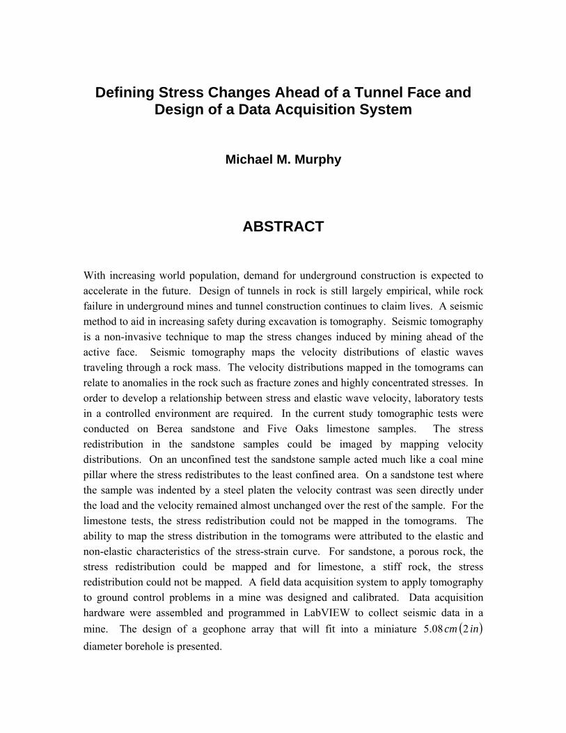
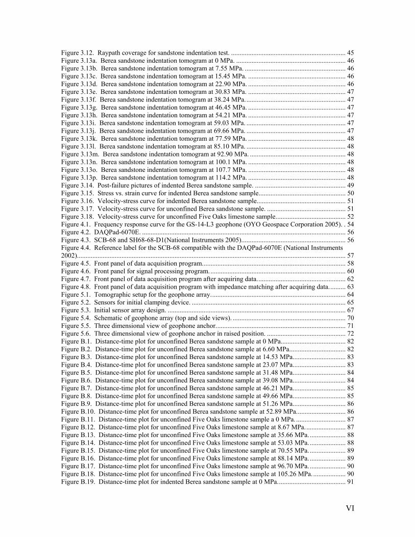
The conclusions from the study are that the low velocity zones observed in the initial tomograms show pre-existing fractures within the sample. The indentation load (warm color at the top of the figure) was said to be clearly seen in Figures 2.11e – 2.11f. However, the location of the indentation does not appear to be position shown in Figures 2.11e – 2.11f. Johnson stated the reason for the discrepancy is from eccentric loading of the indentation platen. The loading of one side of the platen more than the other results in the stress condition observed. A picture of the failed sample can be seen in Figure 2.12 and a picture of the loading platform operated by a hand pump can be seen in Figure 2.13 (Johnson 2004).

23

Figure 2.12. Prior (left) and post-failure (right) Five Oaks limestone sample from indentation test.

Figure 2.13. Loading platform operated by a hand pump for Five Oaks limestone indentation test.

24

CHAPTER 3 – LABORATORY TESTING

3.1 Introduction In order to understand and interpret tomographic data in the field, laboratory experiments in a controlled environment are essential. Laboratory tests were conducted in order to develop a relationship between P-wave velocity and stress. Two rocks of different elastic properties and porosities were chosen for comparison. The two rocks chosen were Five Oaks limestone and Berea sandstone. Tomographic data were taken while the samples were loaded under uniaxial compression. Porosity tests were conducted as described in Section 2.1.3 in order to determine the amount of void space present in the two types of rock. The results of the porosity test are shown in Table 3.1.

Table 3.1. Results from porosity test.

SS1 10.11 5.01 3263 429.7 462.8 16.63SS2 10.43 5.00 3357 445.5 479.6 16.64SS3 10.18 5.01 3281 433.5 466.9 16.68SS4 9.08 5.01 2926 381.9 412.7 17.25LS1 9.31 5.01 3009 494.8 494.9 0.05LS2 10.33 5.01 3332 549.2 549.4 0.10LS3 10.41 5.01 3354 551.1 552.2 0.54

Porosity (%)

Wwet

(g)Wdry

(g)Sample L

(cm)D

(cm)Vol

(cm3)

The limestone samples have an effective porosity of 0% and the sandstone samples have a porosity of approximately 17%. Porosities of core samples from the same block of Five Oaks limestone have also been found to be 0% (Johnson 2004).

3.2 Sample Preparation Berea sandstone blocks were obtained from Pioneer Supply, a distributor for Cleveland Quarries located in Parkersburg, West Virginia. The blocks were cut by Cleveland Quarries to an approximate size of cm24.1502.3302.33 ×× ( )in61313 ×× . Pre-preparation by Cleveland Quarries of the sandstone blocks also included grinding of the top and bottom surfaces. The top and bottom surfaces must be parallel in order to conduct uniaxial testing. If the surfaces are not parallel loading the sample will be

25

uneven and inaccurate stress-strain data will be acquired. Figure 3.1 is a sandstone block obtained from Pioneer Supply.

Figure 3.1. Berea sandstone block obtained from Pioneer Supply.

Limestone blocks were collected from the Five Oaks seam at the Kimballton mine located in Pembroke, Va. Blocks with rough dimensions of cm5.300.614.91 ×× ( )ft123 ×× were pried from the rib near a working section. The limestone blocks

were pulled from pillars in the 12 East mains at a depth of m671 ( )ft2200 . A milling machine was used to drill core samples from the sandstone and limestone blocks. Different drilling bits used on the blocks produced cores with length to diameter ratios of 1:1 and 2:1. Sandstone and limestone cores for an unconfined loading test were cored to a diameter of ( )incm 208.5 and a length of ( )incm 416.10 . After the initial core was made with the milling machine a saw with a diamond blade sized the sample length down to approximately ( )incm 416.10 . The top and bottom surfaces of the core were smoothed using a diamond wheel grinder in order to make the surfaces parallel. The smoothness of the surfaces were checked using a dial

26

indicator to see how parallel the faces were within a range of approximately 0.003 inches. A sandstone sample for an indentation test was cored to diameter of

( )incm 624.15 and a length of ( )incm 624.15 . Pre-preparation done by Cleveland Quarries of the larger sandstone core already involved smoothing the surfaces since the height of the sample matched the height of the block.

3.3 Description of Laboratory Experiment The samples were loaded in an MTS loading machine which applied a vertical stress to the cores under displacement control at a rate of sec003.0 mm ( )sec1018.1 4 in−× . The MTS machine was put on hold at different loads so tomographic data could be acquired. The samples were compressed until the peak compressive strength was reached and the sample failed. An ultrasonic data acquisition system developed by Wes Johnson (Johnson 2004) was used in order to collect tomographic data at different loads. In all test samples eighteen sensors were used as receivers and fifteen sensors were used as sources. Piezoelectric transducers manufactured by Panametrics (part #Micro 80) were used in all laboratory testing. The transducers have a frequency range of 175-1000 kHz and could be used interchangeably between source and receiver. A schematic of the equipment used in the laboratory is seen in Figure 3.2. An ultrasonic pulsar was used to generate a square wave through the sample. An ultrasonic switchbox was used allow each source to generate a delayed square wave. A delay is required so all the receivers have ample time to collect the waveform. The receivers passed the waveform onto digital oscilloscopes to convert the signal from analog to digital form. The control of the source triggering and collection of waveforms were controlled in a LabVIEW program. The sensors were mounted on all samples with a cynoacrylate adhesive. An experiment was conducted on the advantages of using a cynoacrylate adhesive and the results are shown in Appendix A. Data were taken while the MTS machine was paused at different loads, starting with no load until sample reached failure.

27

Figure 3.2. Setup of tomographic data collection (Johnson 2004). A ( )incm 208.5 diameter steel platen was used to load the sample during testing. Three-dimensional and two-dimensional tomographic surveys were created for the experiment. For three-dimensional tomographic surveys both sandstone and limestone cores were tested. The ( )incm 208.5 diameter cores of sandstone and limestone were tested under unconfined compression. The sensors and receivers were arranged in a three-dimensional array. A two-dimensional tomographic survey was conducted on the ( )incm 624.15 diameter Berea sandstone sample. The steel platen was used to induce a state of stress on the surface of the sandstone. For the indentation test the sources and receivers were arranged in a two-dimensional array. Due to the number of source-receiver pairs for each experiment 270 waveforms were collected. Arrival times were picked for each waveform using a travel-time picking program created in LabVIEW. The arrival time of a waveform is illustrated in Figure 3.3.

28

Figure 3.3. Example of the arrival time for a waveform. The front panel of the program can be seen in Figure 3.4. The program uses a reference waveform with a known arrival time and attempts to automatically pick the arrival times of the raw data waveforms based upon the pattern of the reference waveform. Inputs required for the program are a reference waveform file, source/receiver coordinate files and the raw data file.

Figure 3.4. Front panel of the time-picking program.

Once the arrival times were found for all the waveforms distance-time plots were created. Distance-time plots and average elastic wave velocity from each load can be seen in Appendix B. Travel-time projections were entered into inversion software called GeoTomCG in order to compute the velocity distributions. The velocity distribution data generated by GeoTomCG was entered into model generation programs called Surfer 7.0 and RockWorks 2004 to better display the tomographic data. Surfer 7.0 was used for the two-dimensional surveys and RockWorks 2004 was used for three-dimensional surveys.

Arrival Time

29

3.4 Berea Sandstone and Five Oaks Limestone Unconfined Loading Test Thirty-three sensors were placed in horizontal and vertical arrays around the rock cores for three-dimensional tomographic survey results. An illustration showing the sensor arrangement and loading conditions on the rock is shown in Figure 3.5. The receivers are shown in blue and the sources are shown in green. A steel platen with a

( )incm 208.5 diameter was used to load the sample. The sample was unconfined during loading.

Figure 3.5. Sensor alignment and loading conditions on unconfined sandstone and limestone samples.

Receiver

Source

All units in centimeters

30

The loads at which tomographic data were acquired for the sandstone and limestone are shown in Table 3.2 and 3.3, respectively. The sandstone and limestone samples failed at approximately 54 MPa )7930( psi and 130 MPa )18850( psi , respectively.

Table 3.2. Loads tomographic data were acquired for the unconfined Berea sandstone test.

Load MPa PSI1 0.00 02 6.60 9553 14.53 21504 23.07 33455 31.48 45356 39.08 57307 46.21 69258 49.66 74009 51.26 764010 52.89 7880

Table 3.3. Loads tomographic data were acquired for the unconfined Five Oaks limestone test.

Load MPa PSI1 0.00 02 8.67 12573 35.66 51704 53.03 76905 70.55 102306 88.14 127807 96.70 140228 105.26 15263

The results from the sandstone and limestone unconfined tests are shown on the following pages. The sandstone tomograms are shown in Figures 3.6a – 3.6j and the limestone tomograms are shown in Figures 3.7a – 3.7h. The figures shown are two cross sections running from East-West and North-South to show the stress redistribution inside of the rock sample during compression. All velocity values in the scale are in ft/sec. The post-failure samples can be seen in Figure 3.8.

31

Figure 3.6a. Berea sandstone unconfined tomogram at 0 MPa.

Figure 3.6b. Berea sandstone unconfined tomogram at 6.60 MPa.

32

Figure 3.6c. Berea sandstone unconfined tomogram at 14.53 MPa.

Figure 3.6d. Berea sandstone unconfined tomogram at 23.07 MPa.

33

Figure 3.6e. Berea sandstone unconfined tomogram at 31.48 MPa.

Figure 3.6f. Berea sandstone unconfined tomogram at 39.08 MPa.

34

Figure 3.6g. Berea sandstone unconfined tomogram at 46.21 MPa.

Figure 3.6h. Berea sandstone unconfined tomogram at 49.66 MPa.

35

Figure 3.6i. Berea sandstone unconfined tomogram at 51.26 MPa.

Figure 3.6j. Berea sandstone unconfined tomogram at 52.89 MPa.

36

Figures 3.7a-3.7h shows the results from the unconfined limestone test.

Figure 3.7a. Five Oaks limestone unconfined tomogram at 0 MPa.

Figure 3.7b. Five Oaks limestone unconfined tomogram at 8.67 MPa.

37

Figure 3.7c. Five Oaks limestone unconfined tomogram at 35.66 MPa.

Figure 3.7d. Five Oaks limestone unconfined tomogram at 53.03 MPa.

38

Figure 3.7e. Five Oaks limestone unconfined tomogram at 70.55 MPa.

Figure 3.7f. Five Oaks limestone unconfined tomogram at 88.14 MPa.

39

Figure 3.7g. Five Oaks limestone unconfined tomogram at 96.70 MPa.

Figure 3.7h. Five Oaks limestone unconfined tomogram at 105.26 MPa.

40

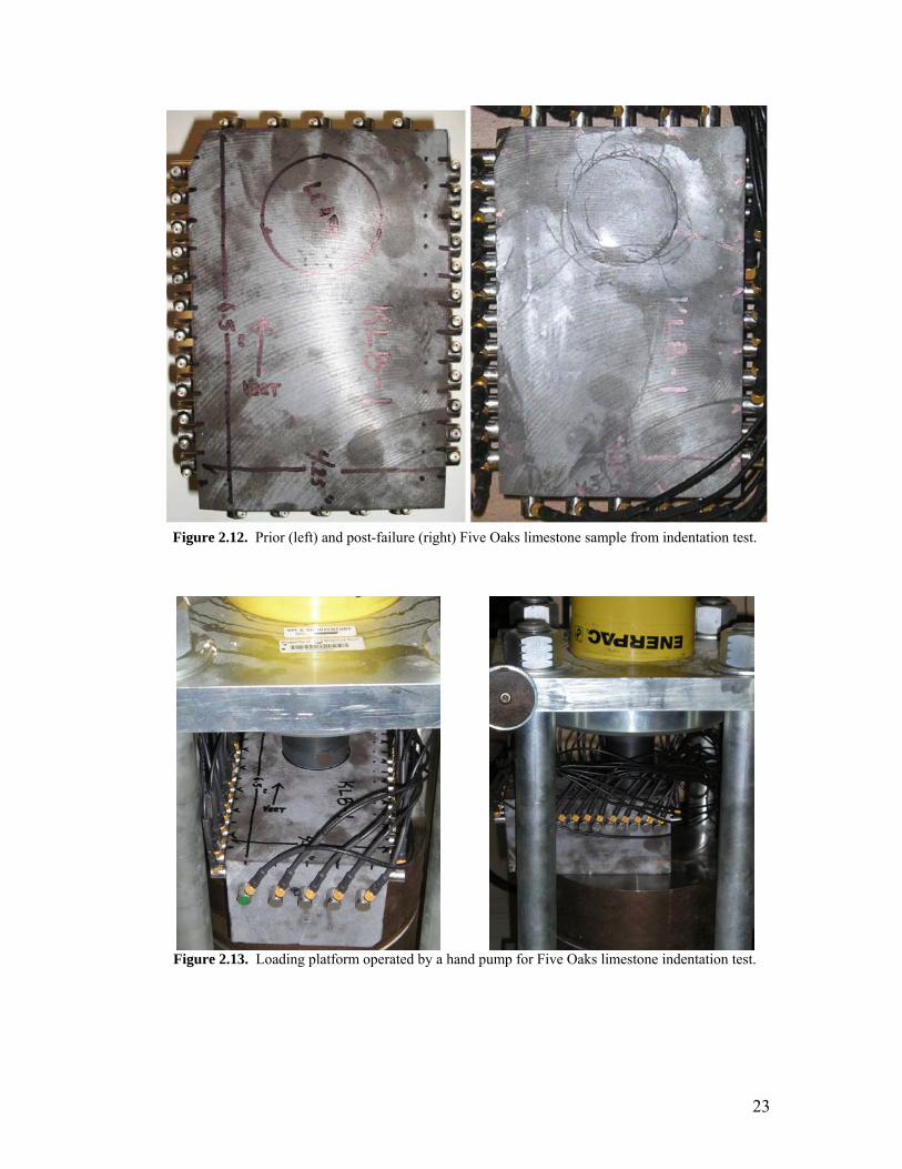
Figure 3.8. Post-failure sandstone (left) and limestone (right) samples from unconfined test.

The results from the unconfined Berea sandstone tests shown in Figures 3.6a-3.6j show similar results to the stress redistribution during loading seen in a coal mine pillar (Wagner 1974). The corners of a coal mine pillar are the least confined portion whereas the centers of the pillar are subjected to the greatest confinement. Stress is simply defined as force per unit area therefore in theory the stress concentration in the corners should be higher due to the lesser amount of confinement. Wagner showed that up until overall pillar failure the stress distribution follows closely with theory whereas high stress concentrations are near the corners of the pillar and low stress levels are in the center. In the results found for the unconfined Berea sandstone test, Figure 3.6d starts to show high velocities being concentrated on the outer edge of the cylindrical sample whereas the core has relatively lower velocity. The high velocities starting to form are indicative of the higher stressed area on the outer edge. Figures 3.6g through 3.6j show dominant higher velocities on the outer edge whereas the inner core has the same approximate velocity as Figure 3.6d. The progression of the tomograms shows higher velocities concentrating around the outer edges of the Berea sandstone sample which is indicative of the stress redistributing to the outer edge during loading.

41

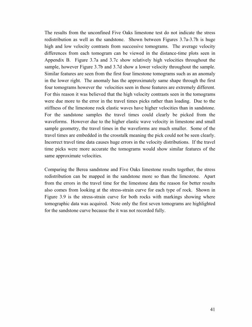
The results from the unconfined Five Oaks limestone test do not indicate the stress redistribution as well as the sandstone. Shown between Figures 3.7a-3.7h is huge high and low velocity contrasts from successive tomograms. The average velocity differences from each tomogram can be viewed in the distance-time plots seen in Appendix B. Figure 3.7a and 3.7c show relatively high velocities throughout the sample, however Figure 3.7b and 3.7d show a lower velocity throughout the sample. Similar features are seen from the first four limestone tomograms such as an anomaly in the lower right. The anomaly has the approximately same shape through the first four tomograms however the velocities seen in those features are extremely different. For this reason it was believed that the high velocity contrasts seen in the tomograms were due more to the error in the travel times picks rather than loading. Due to the stiffness of the limestone rock elastic waves have higher velocities than in sandstone. For the sandstone samples the travel times could clearly be picked from the waveforms. However due to the higher elastic wave velocity in limestone and small sample geometry, the travel times in the waveforms are much smaller. Some of the travel times are embedded in the crosstalk meaning the pick could not be seen clearly. Incorrect travel time data causes huge errors in the velocity distributions. If the travel time picks were more accurate the tomograms would show similar features of the same approximate velocities. Comparing the Berea sandstone and Five Oaks limestone results together, the stress redistribution can be mapped in the sandstone more so than the limestone. Apart from the errors in the travel time for the limestone data the reason for better results also comes from looking at the stress-strain curve for each type of rock. Shown in Figure 3.9 is the stress-strain curve for both rocks with markings showing where tomographic data was acquired. Note only the first seven tomograms are highlighted for the sandstone curve because the it was not recorded fully.

42

0

20

40

60

80

100

120

140

0 0.001 0.002 0.003 0.004 0.005 0.006 0.007 0.008 0.009 0.01

Strain

Stre

ss (M

pa)

Sandstone Limestone

Figure 3.9. Stress vs. strain curves for Berea sandstone and Five Oaks limestone.

The stress-strain curve for the sandstone shows a gradual increase in tangential Young’s modulus as loading increases. The curve is only approximately linear during strain values of 0.006 and 0.008. A complete stress-strain curve from another test with the same sample size and load configuration as the current experiment can be seen in Figure 3.10. Figure 3.10 shows that close to the end of the stress-strain curve for Berea sandstone the curve becomes gradually non-linear again. The increase and decrease in tangential Young’s modulus throughout of the curve is attributed to the closing of pore space and introduction of microfractures during loading. The tomograms for the Berea sandstone test are able to show clear velocity changes indicative of stress changes because of the characteristics of the stress-strain curve.

43

Stress vs. Strain Curve for Berea Sandstone

0

10

20

30

40

50

60

0 0.001 0.002 0.003 0.004 0.005 0.006 0.007 0.008 0.009

Strain

Str

ess

(MP

a)

Figure 3.10. Complete stress vs. strain curve for Berea sandstone.

The stress-strain curve for the limestone sample in Figure 3.9 shows non-elastic characteristics during initial loading. This portion of the curve is non-linear and represents the closing of microfractures already present in the sample. Although the effective porosity is 0% there are still microfractures present in the rock sample. No significant change in velocity was seen in the tomograms during this portion of the stress-strain curve. The stress-strain curve then becomes very elastic and linear until failure is reached at the peak of the curve. Failure is sudden for the Five Oaks limestone because there is no non-linear portion before the peak. This characteristic seen in the limestone curve is unlike the Berea sandstone curve seen in Figure 3.10. The tomograms for the Five Oaks limestone sample reflect no real stress redistribution because most of the curve is fairly linear. The only way to see velocity change in the limestone tomograms would be due to heavy fracturing during loading. If the limestone core had a larger diameter the distances between the source and receivers would increase. The increase in distance would make the travel times larger and the arrival time would be picked more accurately in the waveform.

44

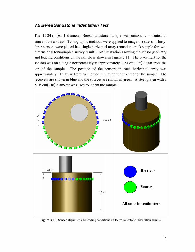
3.5 Berea Sandstone Indentation Test The ( )incm 624.15 diameter Berea sandstone sample was uniaxially indented to concentrate a stress. Tomographic methods were applied to image the stress. Thirty-three sensors were placed in a single horizontal array around the rock sample for two-dimensional tomographic survey results. An illustration showing the sensor geometry and loading conditions on the sample is shown in Figure 3.11. The placement for the sensors was on a single horizontal layer approximately cm54.2 ( )in1 down from the top of the sample. The position of the sensors in each horizontal array was approximately °11 away from each other in relation to the center of the sample. The receivers are shown in blue and the sources are shown in green. A steel platen with a

( )incm 208.5 diameter was used to indent the sample.

Figure 3.11. Sensor alignment and loading conditions on Berea sandstone indentation sample.

Receiver

Source

All units in centimeters

45

The steel platen was placed off center due to raypath coverage going through the center of the sample. As can be seen in Figure 3.12, the center of the sample has no raypath coverage. The concentration of the most raypaths appear to be midway between the center and edge of the sample. The platen was located in that area for best tomographic results.

Figure 3.12. Raypath coverage for sandstone indentation test.

The loads at which tomographic data were taken are shown in Table 3.4. The six-inch diameter Berea sandstone sample failed at approximately 114 MPa ( )psi16560 . The last tomogram was taken before the sample completely failed.

Table 3.4. Loads tomographic data were acquired for sandstone indentation sample. Load MPa PSI

1 0.00 02 7.55 10953 15.45 22404 22.90 33205 30.83 44706 38.24 55457 46.45 67358 54.21 78609 59.03 8560

10 69.66 1010011 77.59 1125012 85.10 1234013 92.90 1347014 100.07 1451015 107.72 1562016 114.21 16560

46

Tomograms created in Surfer 7.0 can be seen in Figures 3.13a – 3.13p. A picture of the rock after failure can be seen in Figure 3.14. All velocity values in the scale are in units of ft/sec.

Figure 3.13a. Berea sandstone indentation tomogram at 0 MPa.

Figure 3.13b. Berea sandstone indentation tomogram

at 7.55 MPa.

Figure 3.13c. Berea sandstone indentation tomogram at 15.45 MPa.

Figure 3.13d. Berea sandstone indentation tomogram

at 22.90 MPa.

.1

47

Figure 3.13e. Berea sandstone indentation tomogram at 30.83 MPa.

Figure 3.13f. Berea sandstone indentation tomogram at 38.24 MPa.

Figure 3.13g. Berea sandstone indentation tomogram at 46.45 MPa.

Figure 3.13h. Berea sandstone indentation tomogram at 54.21 MPa.

Figure 3.13i. Berea sandstone indentation tomogram at 59.03 MPa. Figure 3.13j. Berea sandstone indentation tomogram

at 69.66 MPa.

48

Figure 3.13k. Berea sandstone indentation tomogram at 77.59 MPa.

Figure 3.13l. Berea sandstone indentation tomogram

at 85.10 MPa.

Figure 3.13m. Berea sandstone indentation tomogram

at 92.90 MPa.

Figure 3.13n. Berea sandstone indentation tomogram

at 100.1 MPa.

Figure 3.13o. Berea sandstone indentation tomogram

at 107.7 MPa.

Figure 3.13p. Berea sandstone indentation tomogram

at 114.2 MPa.

49

Figure 3.14. Post-failure pictures of indented Berea sandstone sample.

The tomographic surveys for the ( )incm 624.15 diameter Berea sandstone sample illustrates an increase in velocity where the load is applied. The change in velocity can start to be seen in Figure 3.13d and is predominant by Figure 3.13l. The change in velocity at the platen location is indicative of a change of stress during loading. The surrounding area where no load is applied is characterized by an almost constant velocity in most of the tomograms. The velocity is near constant in the surrounding areas because no load was present. The location of the high velocity areas in the tomograms and the location of the platen shown in Figure 3.11 are slightly different. The reason is because the sample was centered with the vertical force instead of the platen. Since the vertical force was more centered with left edge of the platen it received a higher force than the right edge. The tomograms indicate this by showing the stressed areas shifted slightly left in relation to the platen location. Artifacts are seen in the tomograms for the Berea sandstone sample. Artifacts are typically characterized by areas around the edge of the tomogram with extremely high or low velocities. The occurrence of artifacts has been linked to the limitations of source-receiver geometry and the reconstruction algorithms used (Saito and Ohtomo 1987). In Figures 3.13e – 3.13p two artifacts around the edge showing a large velocity area become more and more visible as load increases. If these high velocity areas are correlated with the sensor array geometry it can be seen that the artifacts consistently occur approximately where sources and receivers are directly beside each other. The artifacts are believed to be caused by inaccurate arrival time picks. The arrival times for the waveforms in these areas are embedded in the crosstalk of the

Top View – Platen area highlighted

50

signal due to the short travel path. The stress-strain curve is shown in Figure 3.15 for the indented ( )incm 624.15 diameter Berea sandstone sample. Like the previous Berea sandstone curves (Figure 3.9 and 3.10) the curve shows heavy non-linear trends at the beginning and end.

Stress vs. Strain Curve for Indented Berea Sandstone

0

20

40

60

80

100

120

0 0.001 0.002 0.003 0.004 0.005 0.006 0.007 0.008

Strain

Stre

ss (M

Pa)

Figure 3.15. Stress vs. strain curve for indented Berea sandstone sample.

The results from the Five Oaks limestone block test discussed in Section 2.5 doesn’t indicate as clear of a concentrated velocity change due to stress underneath the platen as the Berea sandstone results. The limestone block test shows an initial fracture, see Figure 2.11a, propagating from the bottom moving upwards and to the left. As loading continues, the fracture becomes more and more prominent until Figure 2.11f. A stress-strain curve could not be obtained with the limestone block because the sample was indented with a hand pump. With stiffer rocks it’s difficult to see the stress redistribution however with a bigger limestone sample a fracture can clearly be seen in the tomograms. Average velocity-stress plots were created for the conducted experiments. The plots for the Berea sandstone tests can be seen in Figures 3.16 and 3.17 and the plot for the Five Oaks limestone test can be seen in Figure 3.18.

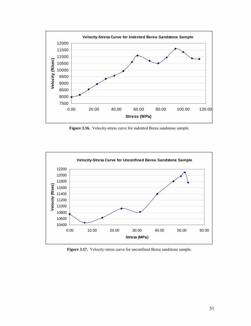
51

Velocity-Stress Curve for Indented Berea Sandstone Sample

75008000850090009500

1000010500110001150012000

0.00 20.00 40.00 60.00 80.00 100.00 120.00

Stress (MPa)

Velo

city

(ft/s

ec)

Figure 3.16. Velocity-stress curve for indented Berea sandstone sample.

Velocity-Stress Curve for Unconfined Berea Sandstone Sample

104001060010800

11000112001140011600

118001200012200

0.00 10.00 20.00 30.00 40.00 50.00 60.00

Stress (MPa)

Vel

ocity

(ft/s

ec)

Figure 3.17. Velocity-stress curve for unconfined Berea sandstone sample.

52

Velocity-Stress Curve for Unconfined Five Oaks Limestone Sample

1500016000170001800019000200002100022000230002400025000

0.00 20.00 40.00 60.00 80.00 100.00 120.00

Stress (MPa)

Velo

city

(ft/s

ec)

Figure 3.18. Velocity-stress curve for unconfined Five Oaks limestone sample.

The two velocity-stress curves for the Berea sandstone samples show large increases in average velocity initially and decreases in average velocity towards sample failure. These characteristics are attributed to the features seen in the stress-strain curve which are the closure of pore space and introduction of microfractures. The velocity-stress curve shows large difference between each point and is attributed to error in the travel time picks. Small errors in arrival time picking can lead to large velocity distribution errors seen in the tomograms.

53

CHAPTER 4 – DATA ACQUISITION AND LABVIEW PROGRAMMING

4.1 Data Acquisition System Hardware The design and calibration of a data acquisition system to be used in the field for defining elastic wave velocity changes within the rock ahead of the mining face due to excavation is to be analyzed. One of the most important parameters in selecting a sensor for acquisition of data is the operating frequency. As stated in Section 2.2.6, Equation 2.7 shows the frequency of a seismic signal ( )f is a function of the

wavelength ( )λ and wave velocity inside of the medium ( )v and is related by the expression:

fv=λ

Sensors will be implemented in a hard rock mine for acquiring seismic signals. In a the hard rock mine, such as a limestone mine, the source for the seismic signal will be a rotary percussion drill-bit. Mining equipment such as longwall shearers has been used in the past to generate seismic signals (Rigby et al. 1989; Westman et al. 1996). Longwall shearers were found to give off frequencies in the range of 80-200 Hz. The use of rotary drill bit vibrations as an energy source has been widely utilized (Deily et al. 1968; Lutz et al. 1972). A study found that the frequency range from a drill-bit source was in the range of 25-100 Hz (Rector and Marion 1991). Therefore since the frequency range of the source is unknown at this point a geophone will be selected based upon previous studies. The geophone selected for the experiment is the GS-14-L3 manufactured by OYO Geospace Corporation. A specifications table for the GS-14-L3 can be seen in Table 4.1. The GS-14-L3 is a miniature, self-generating velocity detector designed for rugged environments and can withstand extreme shock with no change in performance characteristics. The bandwidth of the GS-14-L3 is between 24-3000 Hz which matches well with what previous studies have seen for equipment generated seismic sources.

54

Table 4.1. Specifications for the GS-14-L3 Functional Mechanical

Sensitivity ( ± 15%) 290 mV/ips Height 0.68 in Natural Frequency ( ± 20%) 28 Hz Diameter 0.66 in

Bandwidth 24-3000 Hz Weight 0.67 oz Coil Resistance ( ± 5%) 570 ohms Environmental

Coil Inductance 45 mh Operating Temperature -45° to 100°C Damping Factor ( ± 30%) 0.18 Storage Temperature -45° to 100°C

Damping Constant 172 Shock 5000 G Displacement Limit 0.09 in

Inertial Mass 0.076 oz Orientation Angle ± 180°

The frequency response chart provided by OYO Geospace Corporation for the geophone is shown in Figure 4.1.

Figure 4.1. Frequency response curve for the GS-14-L3 geophone (OYO Geospace Corporation 2005).

55

The frequency range of the sensors is important in the selection of the appropriate analog to digital converter because of the Nyquist criterion. Data acquisition hardware had to be selected such that it was able to receive seismic data from the source simultaneously through multiple channels without losing content due to sampling error. Ultimately the system will be implemented for field testing in an underground mine and a requirement for approximately sixteen channels must be met. The requirement of sixteen channels comes from the length of production boreholes at a mine testing where testing will be conducted. The National Instruments DAQPad-6070E and SCB-68 connector block was chosen as the data acquisition hardware. The DAQPad-6070E will be the analog to digital converter which converts the analog signals acquired in the field to digital form. The DAQPad-6070E is a switchless, jumperless enhanced multifunction input/output device that uses a data acquisition system timing controller chip. The specifications for the device are shown in Table 4.2.

Table 4.2. Specifications for the DAQPad-6070E. Bus IEE 1394

Analog Inputs 16 Single Ended/8 DifferentialInput Resolution 12 bits

Max Sampling Rate 1.25 MS/sInput Range ±0.05 to ± 10 V

Analog Outputs 2Output Resolution 12 bits

Output Rate 1 MS/sOutput Range ± 10 V

Digital I/O 8Counter/Timers 2

Triggers Analog, Digital

The maximum sampling rate of the DAQPad is 1.25 MS/s. Acquiring data with sixteen channels would result in a sampling rate of 78.1 kS/s for each channel. This sampling rate is well above the frequency range of interest from the drill-bit energy source. Therefore the Nyquist criterion is not violated and accurate results can be achieved. In fact with the current data acquisition system can handle frequencies up to approximately 35-40 kHz. A picture of the DAQPad can be seen in Figure 4.2.

56

Figure 4.2. DAQPad-6070E.

The geophones will be wired to a connector block. The SCB-68 is a shielded input/output connector block with 68 screw terminals for connection to the analog to digital converter. The SCB-68 connects to the DAQPad via the National Instruments SH68-68-D1 68-pin I/O connector cable. The connector block and shield cable can be seen in Figure 4.3.

Figure 4.3. SCB-68 and SH68-68-D1(National Instruments 2005). The reference label seen in Figure 4.4 shows the pinouts for the SCB-68 when connected to the DAQPad. As can be seen in Figure 4.4 Pin #68 refers to Channel 0, Pin #34 refers to Channel 8 and so on. Geophones are connected into the connector block through shielded copper wire soldered to the leads of the geophone. Each geophone has two leads, one connecting to a channel pin and one connecting to a ground pin. An example of a grounding pin on the reference label is Pin #67. The

57

whole data acquisition system was interfaced to a ruggedized laptop through an IEEE 1394 (firewire) port.

Figure 4.4. Reference label for the SCB-68 compatible with the DAQPad-6070E (National

Instruments 2002).

4.2 LabVIEW Programming of Data Acquisition System The data acquisition hardware was programmed in LabVIEW which is a graphical programming environment developed by National Instruments. LabVIEW is based on the G programming language for data acquisition and control, data analysis, and data presentation. Instead of programming lines of code such as in C++, LabVIEW

58

programs are coded through built in functions which are wired together and resembles a flowchart. The flow of data and logic is easier to understand and errors in the code can be found quickly. Two LabVIEW programs were written for the project. The first program used the data acquisition hardware assembled in Section 4.1 to acquire data from an array of geophones. Up to sixteen geophones can be used by the program at any given time. The program retrieves a specified amount of data from one or more analog input channels whenever an acquire button is clicked. The program is a timed and buffered acquisition. Time acquisition means that a hardware clock is used to control the acquisition rate for fast and accurate timing. Buffered acquisition means that waveforms are stored in an intermediate memory buffer after data is acquired from the DAQ board. Once the all waveforms are acquired the program retrieves the stored data and displays the waveforms on a chart. The waveforms are saved in a text file after being displayed. Successive waveforms can be acquired again or the program can be terminated. The object of the program is to continuously run and acquire data at the press of a button whenever waveforms need to be recorded. The front panel of the program is shown in Figure 4.5.

Figure 4.5. Front panel of data acquisition program.

59

The controls of the program include device, channels, number of scans, scan rate, and input limits. The device is the hardware which acquires the analog waveform data, which is the DAQPad-6070E. The program can be a single channel or multiple channel data acquisition program and channels are selected by the channel control. The waveforms from all the channels will be shown on the same chart. Multiple channels can be used to acquire data by selecting the successive drop down menus labeled I/O (seen in Figure 4.5) to all the channels which will collect data. Currently Figure 4.5 only shows Channel 0 as the only channel acquiring data. To view each channel individually the waveform graph properties need to be changed and then the channels can be plotted on either an overlay plot or a stacked plot. The stacked plot allows each channel to be viewed on an individual graph. The number of scans and scan rate will set the time of acquisition and samples to be collected. For example, as shown in Figure 4.5, the program is set to acquire 1000 samples in one second. If the number of scans is set to 20,000 and the scan rate is set at 10,000 the program will acquire 20,000 samples in two seconds. The input limits will set the minimum and maximum amplitude measurement for the voltage input. The code for the data acquisition program, shown in Appendix C, is based upon an event structure. An event structure is a method to allow blocks of code to be called upon based on an event, which is often a push of a button by the user. When the program is initially started up it will sit idle until an event is called upon by the user. The full program is set inside of a while loop meaning the program will run continuously until the code which defines the program to terminate is called upon. Within the while loop is the event structure. When the acquire button on the front panel is clicked the block of code seen in Figure C.1 is called upon. The block of code in Figure C.1 shows the acquisition part of the program. The code starts off by configuring the data acquisition system based upon the user inputs described previously. The data acquisition system then reads the data from the channels and plots the data on a waveform graph. After the waveforms are plotted on the graph the data must be saved into a text file. Embedded into the event structure is a sequence structure. A sequence structure is sets of code that execute sequentially. Once data has properly been acquired, which is the first part of the sequence structure, the data is then passed into the second part of the sequence structure where it is saved. The block diagram code for saving a file can be seen in Figure C.2.

60

The program is set up so that multiple acquisitions can be made without stopping the program. Most of what Figure C.2 illustrates is incrementing the number in the data filename. The first acquisition data file is saved as acq1.txt, the next is saved acq2.txt and so on. The point of incrementing a number like this is to allow the program to save multiple acquisitions automatically without the user manually entering in filenames. The full program is terminated based upon an event which is defined by a value change in the stop button on the front panel. The second LabVIEW program was created in order to view the waveforms acquired by each channel in the time and frequency domains. A filter was also placed in the program to increase the signal to noise ratio of the waveform by eliminating unwanted signals. The program performs a Fourier transformation, which allows the waveforms to be seen in the frequency domain. By viewing the waveforms in the frequency domain the user can see what signal frequencies the geophones are acquiring. The front panel of the signal processing program is shown in Figure 4.6.

Figure 4.6. Front panel for signal processing program.

As can be seen in Figure 4.6, the program shows two plots which represent the signals in the time domain (left) and frequency domain (right). The channel selector on the bottom left allows the user to view all the channels in a raw data file one at a

61

time. The channels in the raw data file need to be in columns. The file is loaded by pressing the read file button and the program is terminated by pressing the stop button. The block of code which reads in the file and displays the data is shown in Appendix C as Figure C.3. As can be seen in Figure B.3 the program is inside of a while loop and contains an event structure. An event for when the read file button is pressed calls on the block of code to read and load the data file. The event shown in Figure C.3 is for when the channel button is pressed. The file is indexed to the channel selector, meaning if the first column of the raw data file was selected the program would be displaying the data for Channel 0. The program sets up data to be plotted to a waveform graph. The parameters are the initial time, time interval, and the raw data for the waveform graph. In case any unwanted signals were still coming into the system, a filter was programmed into the signal processing program. The filter was a highpass filter with a cutoff frequency set at 60 Hz. The cutoff frequency was chosen in order to simply eliminate noise from a laboratory environment such as fluorescent lights. When the system is ultimately tested in the mine the filter can be taken out if the drill-bit generates frequencies below 60 Hz. After the filter, a Fourier transformation function is called upon and the data is then displayed in both the time and frequency domains.

4.3 Testing of Data Acquisition System Four GS-14-L3 geophones were used to acquire data in order to test the data acquisition programs. Shielded copper wires were soldered onto the leads of the geophones and then wired to the pins of the SCB-68 connector block. Channels 0-3 of the data acquisition system were used as the active channels for testing. Geophones were put on a hard surface and a hammer tap was used to generate elastic waves. The front panel of the program after data had been acquired is shown in Figure 4.7.

62

Figure 4.7. Front panel of data acquisition program after acquiring data.

As can seen from Figure 4.7 the program successfully acquiring data from all four channels with a amplitude range of approximately 2V. Data was acquired again, only this time the impedance between the hard surface and geophone was matched. A water based gel was applied to the surface of the geophone before it was placed on the hard surface. The results of the second acquisition is shown in Figure 4.8.

63

Figure 4.8. Front panel of data acquisition program with impedance matching after acquiring data.

When comparing Figure 4.7 to 4.8 two things can be noticed. The signal before the hammer tap occurs (the straight line) has less noise in Figure 4.8 therefore the signal to noise ratio is improved. The amplitude range of Figure 4.8 is also significantly higher having a range of approximately 3.5V. Matching the impedance between the hard surface and the geophone was found to be helpful in improving the signal quality. The individual waveform and frequency range for each channel of the data shown in Figure 4.8 can be seen in Appendix D. Channel 3’s waveform, shown in Figure D.3 in the appendix, appears to look different than the other waveforms and is attributed to being the furthest away from the hammer tap. The testing of the data acquisition system showed satisfactory results in acquiring data and multiple channels.

64

CHAPTER 5 – DESIGN OF A GEOPHONE ARRAY FOR TOMOGRAPHIC DATA COLLECTION

5.1 Application of Geophone Array Geophone arrays for boreholes has been created in the past for the collection of seismic data (Bergh et al. 1982). Although most arrays are used for vertical boreholes, arrays created for horizontal boreholes has also been designed (Shreve and Westman 2003). One of the most important factors in the design of the geophone array is to ensure proper coupling between the rock and the geophone. All geophones in the array must be in a straight line an firmly pressed against and coupled with the rock. An array consisting of four geophones has been designed to be used with the multichannel data acquisition system designed in Chapter 4 in order to acquire field data. The geophone arrays can be connected together to create arrays of eight, twelve and sixteen geophones. The geophone array design is unique because it will ultimately be used for small horizontal boreholes with diameters of approximately

( )incm 208.5 . The array will collect seismic signals generated by the drill-bit energy during the creation of production boreholes for blasting. A simple schematic of the in-mine borehole set-up is shown in Figure 5.1.

Figure 5.1. Tomographic setup for the geophone array.

65

The dimensions of the face are approximately m10.614.9 × ( )ft2030× and the

depth of the boreholes are approximately m88.4 ( )ft16 . Horizontal boreholes will be drilled 360° around the active mining face which allows for good tomographic accuracy. The geophone array will be placed inside of the first borehole and the subsequent drilling will produce the seismic signals needed for tomographic data. Once multiple boreholes are drilled, the geophone array can be moved and record seismic data from different face locations. The tomographic results can provide insight to valuable information ahead of the mining face such as the state of stress and heavy fracture locations.

5.2 Initial Sensor Array Design A PVC pipe containing an actuating system and sensors was chosen to be used as a probe for horizontal boreholes. A pneumatic actuating system consisting of three miniature air cylinders was to be used for the initial model. The design of the initial model was to test four sensors in one clamping mechanism in order to see coupling and sensor geometry effects. The four different sensors selected for the clamping device was a pinducer VP-1093 (Valpey Fisher), Nano 30 (Physical Acoustics), and the two air transducers (American Piezo). The diameter of the air transducers were so large that the sides had to be ground in order to make the sensor flush with the outside curvature of the pipe. The air transducers were cheap enough to see whether grinding the sides had an effect on how well they could pick up signals. A picture of the sensors can be seen in Figure 5.2.

Figure 5.2. Sensors for initial clamping device.

Air transducers Nano 30 Pinducer

66

Miniature air cylinders EGZ-16-10 manufactured by Festo USA were selected for the pneumatic actuating mechanism. The air cylinders provides a thrust force of 109 N ( )lbs5.24 at six bar of compressed air pressure. The total length of the miniature air

cylinders is approximately ( )inmm 28.15.32 with a stroke of ( )inmm 40.010 . Appropriate T-connectors and tubing were also purchased from Festo USA to allow three miniature cylinders to be put in series. The main criterion governing the selection of the miniature air cylinders were the size, force and the ease of mounting inside of the PVC pipe. The initial sensor array design can be seen in Figure 5.3.

67

Figure 5.3. Initial sensor array design.

68

The PVC pipe was cut to split the upper and lower halves down the middle. The upper half of the PVC pipe contained the different sensors. Holes were drilled so that the sensors could be flush with the outer curvature of the PVC pipe. A manifold was placed on the lower half of the PVC pipe so that the air cylinders could be set in place. The cylinders were threaded and screwed into drillholes that were made on the manifold. The piston of the air cylinder was attached to the top of the PVC pipe using a cynoacrylate adhesive. T-connectors were attached to the bottom of each air cylinder and tubing connected the cylinders in series. Compressed air was injected into the tubing and the upper half of the PVC pipe ascended causing the cylinders to press against the borehole wall. When the sensor array was to be placed inside of a horizontal borehole a water based gel would be put on the outside of the PVC pipe at the sensor locations. Therefore a proper coupling would exist between the sensors and the rock. The main drawbacks of the design were the size of the clamping device and selected sensors. The prototype was designed for a PVC pipe with a ( )incm 362.7 outside diameter. Although it was known the boreholes were smaller, the idea of the design was still to be tested. With the current PVC pipe size chosen, the tubing and accessories were all able to fit well inside of the pipe. The design of the air cylinders allowed the top half to ascend and the sensors were flush with the inside of a previously made concrete borehole. However if the design was sized down to the field boreholes space becomes a huge limitation and the design will not work. Air cylinders were looked into which contained a side inlet for tubing which would eliminate the need for the T-connections and conserve space. However connecting three air cylinders with side inlets in series was found to be a problem. No air cylinders of the desired size were found with side inlets on both sides of the cylinder, which would have been ideal. Initially the piezoelectric sensors seemed to be a good choice for acquiring seismic data until the energy generated by the drill-bit was taken into account. Drill-bit energy from previous studies showed frequencies predominantly in the 25-100 Hz range. Therefore ultrasonic transducers would not be the right choice of sensors to use in the field. Geophones however can pick up the signals in the desired frequency range. The geophone diameter size might interfere with the current layout of the clamping device. The curvature of the borehole would now allow the geophone to be flush in the design presented unless the geophone was attached a different way. Based upon the problems found in the initial sensor design, a new sensor design using geophones was developed.

69

5.3 Final Geophone Array Design Based upon the limitations found in the initial clamping device design, a new design was made for geophones and specifications of the field boreholes. The previous design also placed sensors just a couple inches apart to test the idea, however the new design will allow the sensors to be placed cm48.30 ( ft1 ) apart which is desired for good tomographic precision. A schematic of the new design is seen in Figure 5.4. Complete geophone array dimensions and sensor spacing can be seen in Appendix E. A PVC pipe with an outside diameter of cm83.4 ( in90.1 ) and an inside diameter of

cm09.4 ( in61.1 ) was chosen to contain the assemblies of the clamping mechanism. As seen in Figure 5.4a a double acting air cylinder provides the mechanism to allow the geophones to be raised. Rods are created of the same diameter of the air cylinder piston. The rod extensions are attached to the end of the piston and long enough to reach the two outer geophones. As seen in Figure 5.4b, the rod extensions are bent at the ends of the piston in order to give space for the geophone. When the air cylinder is injected with air the rod on the left side moves outwards while the rod on the right side movies inwards.

70

Figure 5.4. Schematic of geophone array (top and side views).

(a) Side View

(b) Top View (with PVC pipe)

71

Geophone anchors were created with pivot points. A block is attached to the bottom of the PVC pipe to hold the whole unit in place. Mechanical arms are pop riveted to the block and each other. By attaching the arms this way, it allows them to move much like a scissor jack. The pivot points between the two mechanical arms on each side of the geophone are attached to the rod extensions. Therefore when the pivot points are moved left or right the geophone is able to move up and down. A three-dimensional view of a sensor anchor can be seen in Figure 5.5.

Figure 5.5. Three dimensional view of geophone anchor.

The complete geophone anchor dimensions can be seen in Appendix E. The only dimensions that are permanent that are seen in Appendix E are the sensor spacing and geometry of the PVC pipe. Shown in Figure E.2 are the two outer geophones are located ( )incm 624.15 from the edge of the PVC pipe. When successive probes are connected together this allows for the outer sensors in each probe to be

( )ftcm 148.30 apart. A sensor anchor prototype was developed based upon the suggested dimensions shown in Appendix E with relative ease. The mechanical arms of the prototype were made from cabinet hinges and the block was made from a square rod of steel.

Pivot Point

Geophone (GS-14-L3)

Block

Arm

72

Figure 5.6. Three dimensional view of geophone anchor in raised position.

A three-dimensional view of the raised geophone can be seen in Figure 5.6. The pivot point is moved inwards and the geophone ascends. Originally a hole in the PVC pipe directly above the anchor would allow the geophone go to outside of the pipe and press against the rock. A better way to couple the geophone with the rock however is to cut out a hole on top of the PVC pipe. The piece of PVC pipe that was cut out would be glued to the geophone itself. When the geophone ascends now, the curvature of the PVC pipe matches the borehole wall. Seismic signals traveling through a PVC pipe in the past has shown little or no loss of energy (Shreve and Westman 2003). A water based gel will be placed on the top of the pipe before the probe is inserted into the borehole to match the impedance. Air tubing and shielded copper wires will go through the pipe to connect the air cylinders to compressed air and geophones to the connector block, respectively.

Pivot point moved inward causes geophone to ascend.

73

CHAPTER 6 – CONCLUSIONS AND RECOMMENDATIONS

Laboratory studies and literature review of field studies conducted in different mines has shown that tomography has the ability to image the stress redistribution and fractured areas inside of a rock mass. In the current project laboratory tomography tests were conducted on Berea sandstone and Five Oaks limestone samples of different loading configurations and sample sizes. An unconfined loading test was conducted on both sandstone and limestone samples with a length to diameter ratio of 2:1. Results from the Berea sandstone unconfined test showed that the stress redistribution inside of the sample acted similar to the stress redistribution inside of a coal pillar. Highly stressed areas were indicated by high velocity areas on the edge of the sample and low stressed areas indicated by low velocity areas were found in the core of the sample as loading increased. The stress redistribution behavior was attributed to the amount of confinement in the sample. The elastic wave velocity mapped in the limestone sample was very poor. The tomograms generated for the unconfined loading experiment showed large velocity changes between each tomogram and no observable patterns were found. The errors found in the limestone tomograms were attributed to the speed of the elastic wave and errors in the travel time projections. The travel times of some of the waveforms during the limestone experiment were embedded in the crosstalk of the signal. The three-dimensional tomographic results of unconfined tests for both sandstone and limestone were compared in relation to the characteristics of the stress-strain curve. The stress-strain curve for the sandstone show dominant inelastic characteristics initially which are attributed to the closing of pore space. The tangential Young’s modulus increases greatly during this part of the stress-strain curve and the rock becomes stiffer. The velocity distributions in the tomograms were mapped because of the stress-strain curve characteristics. The stress-strain curve for the limestone show dominant elastic characteristics meaning the tangential Young’s modulus was not increasing as much during loading. If the travel times of the limestone were picked correctly it is believed that the tomograms at different loads would show similar velocities throughout the sample until failure. Larger limestone samples with a 2:1 length to diameter ratio should be tested under unconfined loading.

74

Two-dimensional tomographic tests were conducted on a Berea sandstone sample with a 1:1 length to diameter ratio. The Berea sandstone sample was made large enough so that an indentation from a steel platen could induce a state of stress. The effect of the stress could be seen clearly in the tomograms up until failure was reached. A previous indentation test was conducted on a limestone block which showed no real velocity redistribution. However a fracture was seen in the initial tomogram and the propagation and expansion of that fracture was seen in the successive tomograms. Between the two sets of tomographic tests it was concluded that porous rocks like sandstone are good for seeing the stress redistribution. The stress redistribution in stiffer rocks, such as limestone, cannot be indicated as easily however heavily fractured areas can be seen. Tomography is a useful tool to give insight into the behavior of different rocks during loading. The design and calibration of a data acquisition system was presented in this study. The future applications of the data acquisition system are to map stresses changes ahead of a mining face during excavations. The data acquisition system was programmed in LabVIEW and tested using four geophones, however up to sixteen geophones can be used. Testing of the data acquisition system showed better results when the geophones were coupled with a hard surface. By coupling the geophones with the hard surface the impedance between the two media were matched and no energy from the elastic wave generated by a hammer tap was lost. The importance of matching the impedance between the geophone and borehole was stressed for future studies. A geophone clamping mechanism has been designed. For field studies in the future the geophones will be placed ( )incm 208.5 diameter horizontal borehole and must be coupled securely with the borehole wall. A design of coupling the geophones with the borehole wall was created by using air cylinders to raise the geophone when actuated. Dimensions for the geophone array were suggested. A prototype geophone anchor to house the geophone inside of the probe was created based on the suggested dimensions. The geophones in the design array will be wired to the data acquisition system assembled. In the future the full system will be used to map mining induced stress changes ahead of an active face to give the engineer better insight towards safety concerns.

75

REFERENCES Adams, L.H., and E.D. Williamson (1923). "On the compressibility of minerals and rocks at high

pressures." Journal of the Franklin Institute 195(2): 475-529.

Analog Devices. "Analog-Digital Conversion Handbook." (1994). Prentice Hall.

Anderson, D.L. (1967). "A seismic equation of state." Geophysical Journal of the Royal Astronomical Society 13: 9-30.

Attewell, P.B., and I.W. Farmer (1976). Principles of Engineering Geology. London: Chapman and Hall.

Bergh, S., U. Ekström, et al. (1982). "A vertical borehole geophone array." Geophysics 48(11): 1558-59.

Bieniawski, Z.T. (1984). Rock Mechanics Design in Mining and Tunneling. Boston: A.A. Balkema.

Birch, F. (1960). "The velocity of compressional waves in rocks to 10 kilobars, 1." Journal of Geophysical Research 65: 1083.

Birch, F. (1961a). "Composition of the earth's mantle." Geophysical Journal of the Royal Astronomical Society 4: 295-311.

Birch, F. (1961b). "The velocity of compressional waves in rocks to 10 kilobars, 2." Journal of Geophysical Research 66: 2199-224.

Brace, W.F. (1965). "Some new measurements of linear compressibility of rocks." Journal of Geophysical Research 70(2): 391-98.

Brown, E.T. (1981). Rock Characterization Testing and Monitoring ISRM Suggested Methods. New York: Pergamon Press.

Burr-Brown. "Principles of data acquisition and conversion." (1994). Tucson, AZ: Application Bulletin.

Chow, T., I.L. Meglis, et al. (1995). "Progressive microcrack development in tests on Lac du Bonnet Granite; II, Ultrasonic tomographic imaging." International Journal of Rock Mechanics and Mining Sciences & Geomechanics Abstracts 32(8).

Cook, N.G.W. (1965). "The failure of rock." International Journal of Rock Mechanics and Mining Sciences 2: 389-403.

Cormack, A.M. (1973). "Reconstruction of densities from their projections, with applications in radiological physics." Physics in Medicine & Biology 18(2): 195-207.

Cumerlato, C., V. Stachura, et al. (1988). "Application of refraction tomography to map the extent of blast-induced fracturing." Key Questions in Rock Mechanics: Proceedings of the 29th U.S. Sympsium. Eds. P.A. Cundall, R.L. Sterling and A.M. Starfield. Minneapolis, MN. 691-98.

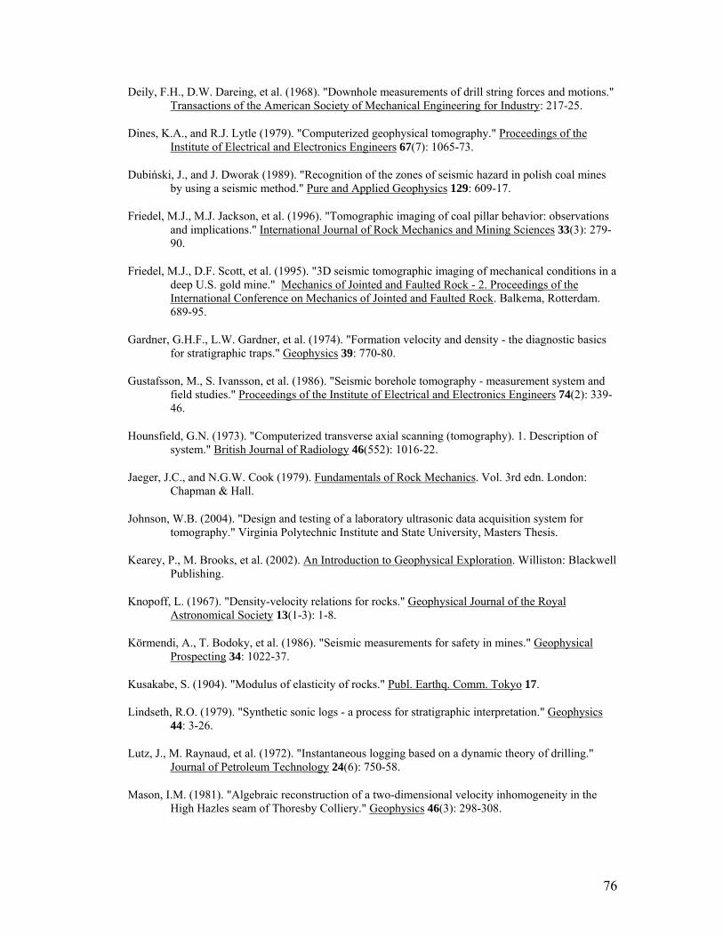
76

Deily, F.H., D.W. Dareing, et al. (1968). "Downhole measurements of drill string forces and motions." Transactions of the American Society of Mechanical Engineering for Industry: 217-25.

Dines, K.A., and R.J. Lytle (1979). "Computerized geophysical tomography." Proceedings of the Institute of Electrical and Electronics Engineers 67(7): 1065-73.

Dubiński, J., and J. Dworak (1989). "Recognition of the zones of seismic hazard in polish coal mines by using a seismic method." Pure and Applied Geophysics 129: 609-17.

Friedel, M.J., M.J. Jackson, et al. (1996). "Tomographic imaging of coal pillar behavior: observations and implications." International Journal of Rock Mechanics and Mining Sciences 33(3): 279-90.

Friedel, M.J., D.F. Scott, et al. (1995). "3D seismic tomographic imaging of mechanical conditions in a deep U.S. gold mine." Mechanics of Jointed and Faulted Rock - 2. Proceedings of the International Conference on Mechanics of Jointed and Faulted Rock. Balkema, Rotterdam. 689-95.

Gardner, G.H.F., L.W. Gardner, et al. (1974). "Formation velocity and density - the diagnostic basics for stratigraphic traps." Geophysics 39: 770-80.

Gustafsson, M., S. Ivansson, et al. (1986). "Seismic borehole tomography - measurement system and field studies." Proceedings of the Institute of Electrical and Electronics Engineers 74(2): 339-46.

Hounsfield, G.N. (1973). "Computerized transverse axial scanning (tomography). 1. Description of system." British Journal of Radiology 46(552): 1016-22.

Jaeger, J.C., and N.G.W. Cook (1979). Fundamentals of Rock Mechanics. Vol. 3rd edn. London: Chapman & Hall.

Johnson, W.B. (2004). "Design and testing of a laboratory ultrasonic data acquisition system for tomography." Virginia Polytechnic Institute and State University, Masters Thesis.

Kearey, P., M. Brooks, et al. (2002). An Introduction to Geophysical Exploration. Williston: Blackwell Publishing.

Knopoff, L. (1967). "Density-velocity relations for rocks." Geophysical Journal of the Royal Astronomical Society 13(1-3): 1-8.

Körmendi, A., T. Bodoky, et al. (1986). "Seismic measurements for safety in mines." Geophysical Prospecting 34: 1022-37.

Kusakabe, S. (1904). "Modulus of elasticity of rocks." Publ. Earthq. Comm. Tokyo 17.

Lindseth, R.O. (1979). "Synthetic sonic logs - a process for stratigraphic interpretation." Geophysics 44: 3-26.

Lutz, J., M. Raynaud, et al. (1972). "Instantaneous logging based on a dynamic theory of drilling." Journal of Petroleum Technology 24(6): 750-58.

Mason, I.M. (1981). "Algebraic reconstruction of a two-dimensional velocity inhomogeneity in the High Hazles seam of Thoresby Colliery." Geophysics 46(3): 298-308.

77

Maxwell, S.C., and R.P. Young (1996). "Seismic Imaging of Rock Mass Responses to Excavation." International Journal of Rock Mechanics and Mining Sciences & Geomechanics Abstracts 33(7): 713-24.

Menke, W. (1984). "The resolving power of cross-borehole tomography." Geophysical Research Letters 11(2): 105-08.

MSHA (2005a). Distribution of Total Days Lost by Accident Class, Underground Mining, 2000-2004. http://www.cdc.gov/niosh/mining/statistics/injuries.htm

MSHA (2005b). Number and Distribution of Mining Fatalities by Work Location and Type of Incident, 2000-2004. http://www.cdc.gov/niosh/mining/statistics/fatalities.htm

Nafe, J.E., and C.L. Drake (1963). "Chapter 29 - Physical Properties of Marine Sediments." The Sea - Ideas and Observations on Progress in the Study of the Seas. Ed. M.N. Hill. Vol. 3. New York, NY: Interscience Publishers.

National Instruments (2002). SCB-68 68-Pin Shielded Connector Block User Manual. Austin, TX.

National Instruments (2005). Austin, TX. http://www.ni.com/

Nishihara, M. (1957). "Stress-strain relation of rocks (rheological properties of rocks I)." Dioshisha Engineering Review 8(2): 32-54.

Nur, A.M. (1971). "Effects of stress on velocity anisotropy in rocks with cracks." Journal of Geophysical Research 76(8): 2022-24.

Obert, L., and W.I. Duvall (1967). Rock Mechanics and the Design of Structures in Rock. New York: John Wiley & Sons.

Ortlepp, W.D. (1983). "The mechanism and control of rockbursts." Rock Mechanics in Mining Practice. Ed. S. Budavari. Johannesburg: The South African Institute of Mining and Metallurgy.

OYO Geospace Corporation (2005). Seismic Detector Response Curve Output VS. Frequency (GS-14-L3). Houston, TX. http://www.geospacelp.com/c_gs14.shtml

Press, F. (1966). "Seismic velocities." Handbook of Physical Constants. Ed. S.P. Jr. Clark: Geological Society of America, Memoir 97.

Rabcewicz, L. (1964). "The New Austrian Tunneling Method." Water Power: November 1964, pp. 453-457, December 64, pp. 511-515, January 65, pp.19-24.

Radon, J. (1917). "Uber die bestimmung von functionen durch ihre integralwere lange gewisser mannigfaltigkeiten." Ber. Verh. Saechs. Akad. Wiss. 69: 262-67.

Rector, J.W, III , and B.P. Marion (1991). "The use of drill-bit energy as a downhole seismic source." Geophysics 56(5): 628-34.

Rigby, N., P.B. Bolt, et al. (1989). "Development and application of an underground microseismic monitoring system for outburst prone coal mines." The Mining Engineer Nov.: 197-203.

Saito, H., and H. Ohtomo (1987). " An attempt to reduce the occurrence of artifacts in seismic ray tomography " Geophysics 52(3): 440.

78

Scott, D.F., Q. Ma, et al. (1994). "Dynamic stress mapping utilizing ultrasonic tomography." Rock Mechanics Models and Measurements Challenges from Industry. Eds. P.P. Nelson and S.E. Laubach.

Scott, D.F., T.J. Williams, et al. (1998). "Use of seismic tomography to identify geologic hazards in underground mines " The Professional Geologist 35(7): 3-5.

Scott, T.E., Q. Ma, et al. (1993). "Tomographic acoustic velocity changes induced during indentation of Berea sandstone." Eos, Transactions, American Geophysical Union 74(43): 408.

Sharma, P.V. (1986). Geophysical Methods in Geology. 2nd Edition ed. Vol. 2nd Edition. Amsterdam: Elsevier Science Publishing Co., Inc.

Sheriff, R.E., and L.P. Geldart (1983). Exploration Seismology Vol 2: Data-Processing and Interpretation. New York: Cambridge University Press. Reprinted with permission of Cambridge University Press.

Shreve, F.J., and E.C. Westman (2003). "Design and testing of multichannel borehole geophone array." Society for Mining, Metallury and Exploration, Transactions 314: 172-76.

Thill, R.E. (1973). "Acoustic methods for monitoring failure in rock." 14th Symposium on Rock Mechanics. Eds. H.R. Hardy, Jr. and R. Stefanko. New York: American Society of Civil Engineers.

Wagner, H. (1974). "Determination of the complete load-deformation characteristics of coal pillars." Proceedings of the Congress of the International Society for Rock Mechanics, no. 3. Vol. 2. 1076-81.

Walsh, J.B. (1965). "The effect of cracks on the compressibility of rock." Journal of Geophysical Research 70(2): 381-89.

Wawersik, W.R., and C. Fairhurst (1970). "A study of brittle rock fracture in laboratory compression experiments." International Journal of Rock Mechanics and Mining Sciences & Geomechanics Abstracts 7: 561-75.

Westman, E.C. (2004). "Use of tomography for inference of stress redistribution in rock." Industry Applications, IEEE Transactions 40(5): 1413-17.

Westman, E.C., K.Y. Haramy, et al. (1996). "Seismic tomography for longwall stress analysis." Proceedings of the 15th International Conference on Ground Control in Mining. Eds. L. Ozdemir, et al. Golden, CO.

Wong, J. (2000). "Crosshole seismic imaging for sulfide orebody delineation near Sudbury, Ontario, Canada." Geophysics 65(6): 1900-07.

Wyllie, M.R.J., A.R. Gregory, et al. (1956). "Elastic Wave Velocities in Heterogeneous and Porous Media." Geophysics 21(1): 41-70.

Zisman, W.A. (1933). "Young's modulus and Poisson's ratio with reference to geophysical applications." Memoirs of the National Academy of Sciences 19: 653-65.

79

APPENDIX A – COUPLING EXPERIMENT BETWEEN TRANSDUCER

AND ROCK SAMPLE

80

Section 2.2.1 of the literature review stresses the importance of matching the impedance at the boundary between two media so no loss of signal occurs. Coupling effects between the piezoelectric transducers used in the laboratory experiments and a Five Oaks limestone block were analyzed. The effects were analyzed by the amplitude of a waveform signal collected when an ultrasonic wave generated by a source transducer passed through the rock. One source was attached to the rock sample and three receivers acquired the ultrasonic signal. The couplings analyzed were a cynoacrylate adhesive, hot glue, and beeswax. The couplings attached the receiver to the rock. The source was attached to the rock with beeswax during all three tests. The results are shown below in Table A.1.

Table A.1. Effects of different couplings on amplitude. Couplant Amplitude

Cynoacrylate Adhesive ±150-200 mVHot Glue ±50 mVBeeswax ±50 mV

The cynoacrylate adhesive showed the best results. The advantage of using the cynoacrylate adhesive was the high amplitude seen in the waveform and the ease of placement on the rock. The disadvantage of using the cynoacrylate adhesive were the transducers had to be cleaned afterwards before another test could be conducted. The advantages of the hot glue was the quick drying of the glue which allowed the sensor to be placed on the rock within seconds. The low amplitude seen in the waveform however caused the use of hot glue undesirable. No advantages were seen in using the beeswax due to the difficulties of placing the transducer on the rock and the low amplitude seen. The beeswax needed to stay warm while sensors were being placed on the rock. Otherwise the beeswax would become hard and brittle, causing the sensors to become easily uncoupled with the rock surface. A final test was conducted to see the effect on amplitude by using the cynoacrylate adhesive on both the receivers and source. The resulting amplitude was found to be ±400 mV. The amplitude doubled the higher amplitude seen from the previous results, confirming that the cynoacrylate adhesive was the best coupling between the transducers and the rock. The cynoacrylate adhesive proved to improve the signal to noise ratio in the signal significantly that cleaning the sensors after each test was no longer a problem.

81

APPENDIX B – DISTANCE-TIME PLOTS

82

Average Velocity - 10745 ft/sec

0.00E+00

5.00E-06

1.00E-05

1.50E-05

2.00E-05

2.50E-05

3.00E-05

0 0.05 0.1 0.15 0.2 0.25 0.3 0.35

Distance (ft)

Tim

e (s

ec)

Figure B.1. Distance-time plot for unconfined Berea sandstone sample at 0 MPa.

Average Velocity - 10480 ft/sec

0.00E+00

5.00E-06

1.00E-05

1.50E-05

2.00E-05

2.50E-05

3.00E-05

3.50E-05

0 0.05 0.1 0.15 0.2 0.25 0.3 0.35

Distance (ft)

Tim

e (s

ec)

Figure B.2. Distance-time plot for unconfined Berea sandstone sample at 6.60 MPa.

83

Average Velocity - 10640 ft/sec

0.00E+00

5.00E-06

1.00E-05

1.50E-05

2.00E-05

2.50E-05

3.00E-05

3.50E-05

0 0.05 0.1 0.15 0.2 0.25 0.3 0.35

Distance (ft)

Tim

e (s

ec)

Figure B.3. Distance-time plot for unconfined Berea sandstone sample at 14.53 MPa.

Average Velocity - 10925 ft/sec

0.00E+00

5.00E-06

1.00E-05

1.50E-05

2.00E-05

2.50E-05

3.00E-05

0 0.05 0.1 0.15 0.2 0.25 0.3 0.35

Distance (ft)

Tim

e (s

ec)

Figure B.4. Distance-time plot for unconfined Berea sandstone sample at 23.07 MPa.

84

Average Velocity - 10825 ft/sec

0.00E+00

5.00E-06

1.00E-05

1.50E-05

2.00E-05

2.50E-05

3.00E-05

0 0.05 0.1 0.15 0.2 0.25 0.3 0.35

Distance (ft)

Tim

e (s

ec)

Figure B.5. Distance-time plot for unconfined Berea sandstone sample at 31.48 MPa.

Average Velocity - 11400 ft/sec

0.00E+00

5.00E-06

1.00E-05

1.50E-05

2.00E-05

2.50E-05

3.00E-05

0 0.05 0.1 0.15 0.2 0.25 0.3 0.35

Distance (ft)

Tim

e (s

ec)

Figure B.6. Distance-time plot for unconfined Berea sandstone sample at 39.08 MPa.

85

Average Velocity - 11815 ft/sec

0.00E+00

5.00E-06

1.00E-05

1.50E-05

2.00E-05

2.50E-05

3.00E-05

0 0.05 0.1 0.15 0.2 0.25 0.3 0.35

Distance (ft)

Tim

e (s

ec)

Figure B.7. Distance-time plot for unconfined Berea sandstone sample at 46.21 MPa.

Average Velocity - 11970 ft/sec

0.00E+00

5.00E-06

1.00E-05

1.50E-05

2.00E-05

2.50E-05

3.00E-05

0 0.05 0.1 0.15 0.2 0.25 0.3 0.35

Distance (ft)

Tim

e (s

ec)

Figure B.8. Distance-time plot for unconfined Berea sandstone sample at 49.66 MPa.

86

Average Velocity - 12100 ft/sec

0.00E+00

5.00E-06

1.00E-05

1.50E-05

2.00E-05

2.50E-05

3.00E-05

0 0.05 0.1 0.15 0.2 0.25 0.3 0.35

Distance (ft)

Tim

e (s

ec)

Figure B.9. Distance-time plot for unconfined Berea sandstone sample at 51.26 MPa.

Average Velocity - 11770 ft/sec

0.00E+00

5.00E-06

1.00E-05

1.50E-05

2.00E-05

2.50E-05

3.00E-05

0 0.05 0.1 0.15 0.2 0.25 0.3 0.35

Distance (ft)

Tim

e (s

ec)

Figure B.10. Distance-time plot for unconfined Berea sandstone sample at 52.89 MPa.

87

Average Velocity - 23960 ft/sec

0.00E+00

2.00E-06

4.00E-06

6.00E-06

8.00E-06

1.00E-05

1.20E-05

1.40E-05

1.60E-05

0 0.05 0.1 0.15 0.2 0.25 0.3 0.35

Distance (ft)

Tim

e (s

ec)

Figure B.11. Distance-time plot for unconfined Five Oaks limestone sample a 0 MPa.

Average Velocity - 19350 ft/sec

0.00E+00

2.00E-06

4.00E-06

6.00E-06

8.00E-06

1.00E-05

1.20E-05

1.40E-05

1.60E-05

1.80E-05

2.00E-05

0 0.05 0.1 0.15 0.2 0.25 0.3 0.35

Distance (ft)

Tim

e (s

ec)

Figure B.12. Distance-time plot for unconfined Five Oaks limestone sample at 8.67 MPa.

88

Average Velocity - 23730 ft/sec

0.00E+00

2.00E-06

4.00E-06

6.00E-06

8.00E-06

1.00E-05

1.20E-05

1.40E-05

1.60E-05

0 0.05 0.1 0.15 0.2 0.25 0.3 0.35

Distance (ft)

Tim

e (s

ec)

Figure B.13. Distance-time plot for unconfined Five Oaks limestone sample at 35.66 MPa.

Average Velocity - 21470 ft/sec

0.00E+00

2.00E-06

4.00E-06

6.00E-06

8.00E-06

1.00E-05

1.20E-05

1.40E-05

1.60E-05

0 0.05 0.1 0.15 0.2 0.25 0.3 0.35

Distance (ft)

Tim

e (s

ec)

Figure B.14. Distance-time plot for unconfined Five Oaks limestone sample at 53.03 MPa.

89

Average Velocity - 21995 ft/sec

0.00E+00

2.00E-06

4.00E-06

6.00E-06

8.00E-06

1.00E-05

1.20E-05

1.40E-05

1.60E-05

0 0.05 0.1 0.15 0.2 0.25 0.3 0.35

Distance (ft)

Tim

e (s

ec)

Figure B.15. Distance-time plot for unconfined Five Oaks limestone sample at 70.55 MPa.

Average Velocity - 20870 ft/sec

0.00E+00

2.00E-06

4.00E-06

6.00E-06

8.00E-06

1.00E-05

1.20E-05

1.40E-05

1.60E-05

0 0.05 0.1 0.15 0.2 0.25 0.3 0.35

Distance (ft)

Tim

e (s

ec)

Figure B.16. Distance-time plot for unconfined Five Oaks limestone sample at 88.14 MPa.

90

Average Velocity - 18695 ft/sec

0.00E+00

2.00E-06

4.00E-06

6.00E-06

8.00E-06

1.00E-05

1.20E-05

1.40E-05

1.60E-05

1.80E-05

2.00E-05

0 0.05 0.1 0.15 0.2 0.25 0.3 0.35

Distance (ft)

Tim

e (s

ec)

Figure B.17. Distance-time plot for unconfined Five Oaks limestone sample at 96.70 MPa.

Average Velocity - 18145 ft/sec

0.00E+00

2.00E-06

4.00E-06

6.00E-06

8.00E-06

1.00E-05

1.20E-05

1.40E-05

1.60E-05

1.80E-05

0 0.05 0.1 0.15 0.2 0.25 0.3 0.35

Distance (ft)

Tim

e (s

ec)

Figure B.18. Distance-time plot for unconfined Five Oaks limestone sample at 105.26 MPa.

91

Average Velocity - 7970 ft/sec

0.00E+00

1.00E-05

2.00E-05

3.00E-05

4.00E-05

5.00E-05

6.00E-05

7.00E-05

0 0.1 0.2 0.3 0.4 0.5 0.6

Distance (ft)

Tim

e (s

ec)

Figure B.19. Distance-time plot for indented Berea sandstone sample at 0 MPa.

Average Velocity - 8135 ft/sec

0

0.00001

0.00002

0.00003

0.00004

0.00005

0.00006

0.00007

0 0.1 0.2 0.3 0.4 0.5 0.6

Distance (ft)

Tim

e (s

ec)

Figure B.20. Distance-time plot for indented Berea sandstone sample at 7.55 MPa.

92

Average Velocity - 8545 ft/sec

0.00E+00

1.00E-05

2.00E-05

3.00E-05

4.00E-05

5.00E-05

6.00E-05

7.00E-05

0 0.1 0.2 0.3 0.4 0.5 0.6

Distance (ft)

Tim

e (s

ec)

Figure B.21. Distance-time plot of indented Berea sandstone sample at 15.45 MPa.

Average Velocity - 8945 ft/sec

0.00E+00

1.00E-05

2.00E-05

3.00E-05

4.00E-05

5.00E-05

6.00E-05

7.00E-05

0 0.1 0.2 0.3 0.4 0.5 0.6

Distance (ft)

Tim

e (s

ec)

Figure B.22. Distance-time plot for indented Berea sandstone sample at 22.90 MPa.

93

Average Velocity - 9340 ft/sec

0.00E+00

1.00E-05

2.00E-05

3.00E-05

4.00E-05

5.00E-05

6.00E-05

0 0.1 0.2 0.3 0.4 0.5 0.6

Distance (ft)

Tim

e (s

ec)

Figure B.23. Distance-time plot for indented Berea sandstone sample at 30.83 MPa.

Average Velocity - 9570 ft/sec

0.00E+00

1.00E-05

2.00E-05

3.00E-05

4.00E-05

5.00E-05

6.00E-05

0 0.1 0.2 0.3 0.4 0.5 0.6

Distance (ft)

Tim

e (s

ec)

Figure B.24. Distance-time plot for indented Berea sandstone sample at 38.24 MPa.

94

Average Velocity - 9920 ft/sec

0.00E+00

1.00E-05

2.00E-05

3.00E-05

4.00E-05

5.00E-05

6.00E-05

0 0.1 0.2 0.3 0.4 0.5 0.6

Distance (ft)

Tim

e (s

ec)

Figure B.25. Distance-time plot for indented Berea sandstone sample at 46.45 MPa.

Average Velocity - 10600 ft/sec

0.00E+00

1.00E-05

2.00E-05

3.00E-05

4.00E-05

5.00E-05

6.00E-05

0 0.1 0.2 0.3 0.4 0.5 0.6

Distance (ft)

Tim

e (s

ec)

Figure B.26. Distance-time plot for indented Berea sandstone sample at 54.21 MPa.

95

Average Velocity - 11085 ft/sec

0.00E+00

1.00E-05

2.00E-05

3.00E-05

4.00E-05

5.00E-05

6.00E-05

0 0.1 0.2 0.3 0.4 0.5 0.6

Distance (ft)

Tim

e (s

ec)

Figure B.27. Distance-time plot for indented Berea sandstone sample at 59.03 MPa.

Average Velocity - 10700 ft/sec

0.00E+00

1.00E-05

2.00E-05

3.00E-05

4.00E-05

5.00E-05

6.00E-05

0 0.1 0.2 0.3 0.4 0.5 0.6

Distance (ft)

Tim

e (s

ec)

Figure B.28. Distance-time plot for indented Berea sandstone sample at 69.66 MPa.

96

Average Velocity - 10500 ft/sec

0.00E+00

1.00E-05

2.00E-05

3.00E-05

4.00E-05

5.00E-05

6.00E-05

0 0.1 0.2 0.3 0.4 0.5 0.6

Distance (ft)

Tim

e (s

ec)

Figure B.29. Distance-time plot for indented Berea sandstone sample at 77.59 MPa.

Average Velocity - 10935 ft/sec

0.00E+00

1.00E-05

2.00E-05

3.00E-05

4.00E-05

5.00E-05

6.00E-05

0 0.1 0.2 0.3 0.4 0.5 0.6

Distance (ft)

Tim

e (s

ec)

Figure B.30. Distance-time plot for indented Berea sandstone sample at 85.10 MPa.

97

Average Velocity - 11590 ft/sec

0.00E+00

1.00E-05

2.00E-05

3.00E-05

4.00E-05

5.00E-05

6.00E-05

0 0.1 0.2 0.3 0.4 0.5 0.6

Distance (ft)

Tim

e (s

ec)

Figure B.31. Distance-time plot for indented Berea sandstone sample at 92.90 MPa.

Average Velocity - 11340 ft/sec

0.00E+00

1.00E-05

2.00E-05

3.00E-05

4.00E-05

5.00E-05

6.00E-05

0 0.1 0.2 0.3 0.4 0.5 0.6

Distance (ft)

Tim

e (s

ec)

Figure B.32. Distance-time plot for indented Berea sandstone sample at 100.1 MPa.

98

Average Velocity - 10875 ft/sec

0.00E+00

1.00E-05

2.00E-05

3.00E-05

4.00E-05

5.00E-05

6.00E-05

0 0.1 0.2 0.3 0.4 0.5 0.6

Distance (ft)

Tim

e (s

ec)

Figure B.33. Distance-time plot for indented Berea sandstone sample at 107.7 MPa.

Average Velocity - 10825 ft/sec

0.00E+00

1.00E-05

2.00E-05

3.00E-05

4.00E-05

5.00E-05

6.00E-05

0 0.1 0.2 0.3 0.4 0.5 0.6

Distance (ft)

Tim

e (s

ec)

Figure B.34. Distance-time plot for indented Berea sandstone sample at 114.2 MPa.

99

APPENDIX C – LABVIEW PROGRAM CODE

100

Figure C.1. Block diagram code for acquiring data.

101

Figure C.2. Block diagram code for saving waveforms to a text file.

102

Figure C.3. Block diagram code for signal processing program.

103

APPENDIX D – RESULTS FROM DATA ACQUISITION PROGRAM

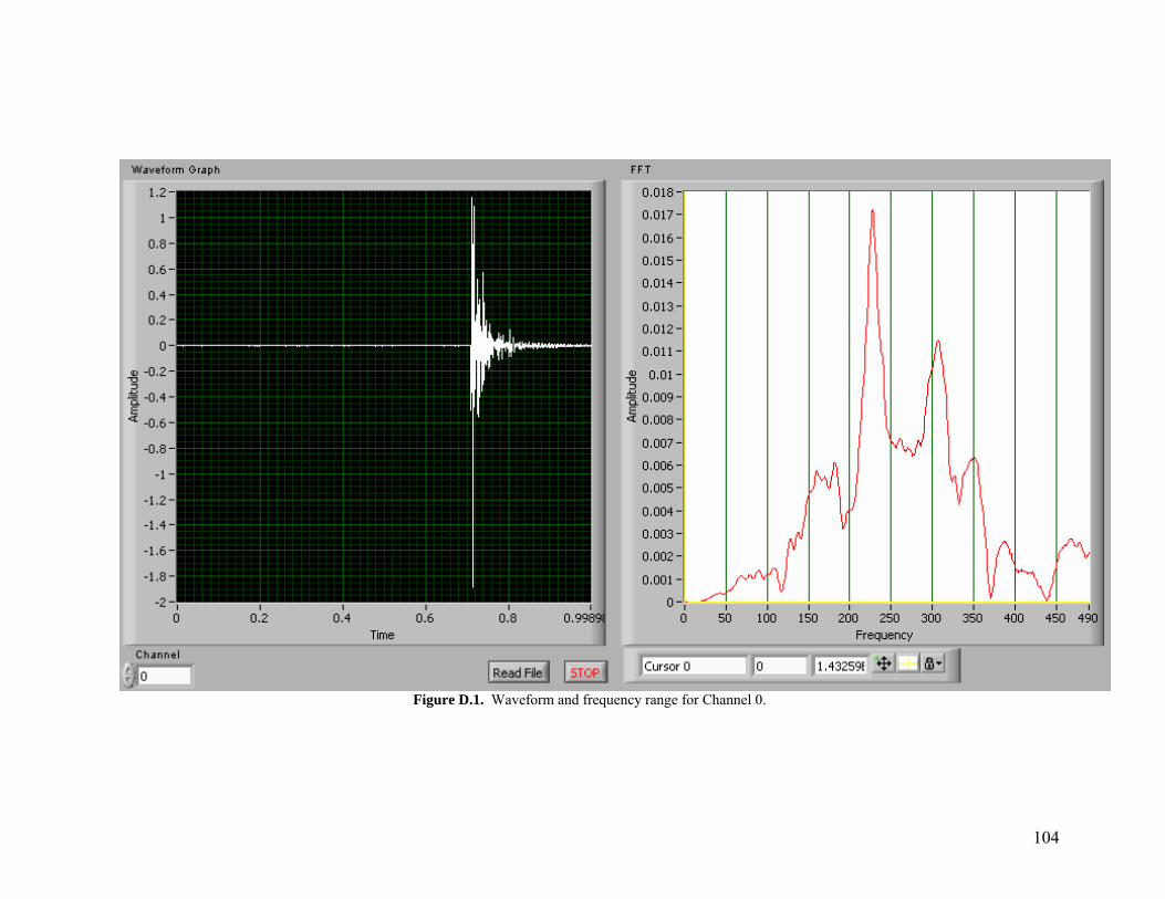
104

Figure D.1. Waveform and frequency range for Channel 0.

105

Figure D.2. Waveform and frequency range for Channel 1.

106

Figure D.3. Waveform and frequency range for Channel 2.

107

Figure D.4. Waveform and frequency range for Channel 3.

108

APPENDIX E – GEOPHONE ARRAY DIMENSIONS

109

Figure E.1. Inside and outside diameters of PVC pipe (units in inches).

Figure E.2. Side view of geophone array showing the spacing between sensors.

110

Figure E.3. Front view dimensions of the sensor anchor.

Figure E.4. Side view dimensions of the sensor anchor.

* approximate

* approximate

111

Figure E.5. Side view of geophone array.

* approximate

Sensor needs to be raised just over 0.55”