defending against internet worms
TRANSCRIPT

DEFENDING AGAINST INTERNET WORMS
By
YONG TANG
A DISSERTATION PRESENTED TO THE GRADUATE SCHOOLOF THE UNIVERSITY OF FLORIDA IN PARTIAL FULFILLMENT
OF THE REQUIREMENTS FOR THE DEGREE OFDOCTOR OF PHILOSOPHY
UNIVERSITY OF FLORIDA
2006

Copyright 2006
by
Yong Tang

I dedicate this to everyone in my family.

ACKNOWLEDGMENTS
First of all, I would like to thank my advisor, Prof. Shigang Chen, for his
guidance and support throughout my graduate studies. Without the numerous
discussions and brainstorms with him, the results presented in this dissertation
would never have existed.
I am grateful to Prof. Sartaj Sahni, Prof. Sanjay Ranka, Prof. Yuguang Fang
and Prof. Dapeng Wu for their guidance and encouragement during my years at
the University of Florida (UF). I would also like to thank Prof. Ye Xia for his
valuable comments and suggestions on my research.
I am thankful to all my colleagues in Prof. Chen’s group, including Qingguo
Song, Zhan Zhang, Wei Pan, Liang Zhang, and MyungKeun Yoon. They provide
valuable feedback for my research.
I would also like to thank many people in the Computer and Information
Science and Engineering (CISE) Department for their help in my research work.
In particular, I would like to thank Fei Wang for his help and valuable discussions
in my research work. I would also like to thank Ju Wang, Zhizhou Wang, Xiaobin
Wu, Mingxi Wu, Jundong Liu and Jie Zhang for their help throughout my graduate
life.
I am also thankful to my long time friends before I entered UF. In particular, I
am thankful to Peng Wu for his help and encouragement.
Last but not least, I am grateful to my parents and sisters for their love,
encouragement, and understanding. It would be impossible for me to express my
gratitude towards them in mere words.
iv
TABLE OF CONTENTS
page
ACKNOWLEDGMENTS . . . . . . . . . . . . . . . . . . . . . . . . . . . . . iv
LIST OF TABLES . . . . . . . . . . . . . . . . . . . . . . . . . . . . . . . . . vii
LIST OF FIGURES . . . . . . . . . . . . . . . . . . . . . . . . . . . . . . . . viii
ABSTRACT . . . . . . . . . . . . . . . . . . . . . . . . . . . . . . . . . . . . x
CHAPTER
1 INTRODUCTION . . . . . . . . . . . . . . . . . . . . . . . . . . . . . . 1
1.1 Internet Worms . . . . . . . . . . . . . . . . . . . . . . . . . . . . . 11.2 Related Work . . . . . . . . . . . . . . . . . . . . . . . . . . . . . . 41.3 Contribution . . . . . . . . . . . . . . . . . . . . . . . . . . . . . . . 6
1.3.1 Distributed Anti-Worm Architecture . . . . . . . . . . . . . . 71.3.2 Signature-Based Worm Identification and Defense . . . . . . 81.3.3 Optimization of Iterative Methods . . . . . . . . . . . . . . . 9
2 SLOWING DOWN INTERNET WORMS . . . . . . . . . . . . . . . . . 10
2.1 Modeling Worm Propagation . . . . . . . . . . . . . . . . . . . . . . 102.2 Failure Rate . . . . . . . . . . . . . . . . . . . . . . . . . . . . . . . 122.3 A Distributed Anti-Worm Architecture . . . . . . . . . . . . . . . . 15
2.3.1 Objectives . . . . . . . . . . . . . . . . . . . . . . . . . . . . 152.3.2 Assumptions . . . . . . . . . . . . . . . . . . . . . . . . . . . 152.3.3 DAW Overview . . . . . . . . . . . . . . . . . . . . . . . . . 172.3.4 Measuring Failure Rate . . . . . . . . . . . . . . . . . . . . . 192.3.5 Basic Rate-Limit Algorithm . . . . . . . . . . . . . . . . . . 202.3.6 Temporal Rate-Limit Algorithm . . . . . . . . . . . . . . . . 222.3.7 Recently Failed Address List . . . . . . . . . . . . . . . . . . 252.3.8 Spatial Rate-Limit Algorithm . . . . . . . . . . . . . . . . . 252.3.9 Blocking Persistent Scanning Sources . . . . . . . . . . . . . 282.3.10 FailLog . . . . . . . . . . . . . . . . . . . . . . . . . . . . . . 302.3.11 Warhol Worm and Flash Worm . . . . . . . . . . . . . . . . 322.3.12 Forged Failure Replys . . . . . . . . . . . . . . . . . . . . . . 33
2.4 Simulation . . . . . . . . . . . . . . . . . . . . . . . . . . . . . . . . 33
v

3 A SIGNATURE-BASED APPROACH . . . . . . . . . . . . . . . . . . . 37
3.1 Double-Honeypot System . . . . . . . . . . . . . . . . . . . . . . . . 373.1.1 Motivation . . . . . . . . . . . . . . . . . . . . . . . . . . . . 373.1.2 System Architecture . . . . . . . . . . . . . . . . . . . . . . . 38
3.2 Polymorphism of Internet Worms . . . . . . . . . . . . . . . . . . . 413.3 Position-Aware Distribution Signature (PADS) . . . . . . . . . . . . 50
3.3.1 Background and Motivation . . . . . . . . . . . . . . . . . . 503.3.2 Position-Aware Distribution Signature (PADS) . . . . . . . . 53
3.4 Algorithms for Signature Detection . . . . . . . . . . . . . . . . . . 573.4.1 Expectation-Maximization Algorithm . . . . . . . . . . . . . 583.4.2 Gibbs Sampling Algorithm . . . . . . . . . . . . . . . . . . . 593.4.3 Complexities . . . . . . . . . . . . . . . . . . . . . . . . . . . 603.4.4 Signature with Multiple Separated Strings . . . . . . . . . . 613.4.5 Complexities . . . . . . . . . . . . . . . . . . . . . . . . . . . 62
3.5 MPADS with Multiple Signatures . . . . . . . . . . . . . . . . . . . 623.6 Mixture of Polymorphic Worms and Clustering Algorithm . . . . . 63
3.6.1 Normalized Cuts . . . . . . . . . . . . . . . . . . . . . . . . . 643.7 Experiments . . . . . . . . . . . . . . . . . . . . . . . . . . . . . . . 66
3.7.1 Convergence of Signature Generation Algorithms . . . . . . . 683.7.2 Effectiveness of Normalized Cuts Algorithm . . . . . . . . . . 693.7.3 Impact of Signature Width and Worm Length . . . . . . . . 703.7.4 False Positives and False Negatives . . . . . . . . . . . . . . 733.7.5 Comparing PADS with Existing Methods . . . . . . . . . . . 75
4 MULTIPLE PADS MODEL AND CLASSIFICATION OF POLYMORPHICWORM FAMILIES: AN OPTIMIZATION . . . . . . . . . . . . . . . . . 78
4.1 Introduction . . . . . . . . . . . . . . . . . . . . . . . . . . . . . . . 784.2 Extraction of Multiple PADS Blocks from the Mixture of Polymorphic
Worms . . . . . . . . . . . . . . . . . . . . . . . . . . . . . . . . . . 804.2.1 PADS Blocks and The Dataset from Byte Sequences . . . . . 804.2.2 Expectation-Maximization (EM) Algorithm . . . . . . . . . . 824.2.3 Extraction of Multiple PADS blocks . . . . . . . . . . . . . . 85
4.3 Classification of Polymorphic Worms and Signature Generation . . 864.3.1 Multiple PADS Blocks Model . . . . . . . . . . . . . . . . . 864.3.2 Classification . . . . . . . . . . . . . . . . . . . . . . . . . . . 89
4.4 Conclusion . . . . . . . . . . . . . . . . . . . . . . . . . . . . . . . . 90
5 SUMMARY AND CONCLUSION . . . . . . . . . . . . . . . . . . . . . . 92
5.1 Summary . . . . . . . . . . . . . . . . . . . . . . . . . . . . . . . . 925.2 Conclusion . . . . . . . . . . . . . . . . . . . . . . . . . . . . . . . . 93
REFERENCES . . . . . . . . . . . . . . . . . . . . . . . . . . . . . . . . . . . 95
BIOGRAPHICAL SKETCH . . . . . . . . . . . . . . . . . . . . . . . . . . . . 100
vi

LIST OF TABLES
Table page
2–1 Failure rates of normal hosts . . . . . . . . . . . . . . . . . . . . . . . . . 14
2–2 5% propagtion time (days) for “Temporal + Spatial” . . . . . . . . . . . 35
3–1 An example of a PADS signature with width W = 10 . . . . . . . . . . . 53
4–1 An example of a PADS block with width W = 10 . . . . . . . . . . . . . 81
4–2 An example of a segment with width W = 10 . . . . . . . . . . . . . . . 82
vii

LIST OF FIGURES
Figure page
2–1 Distributed anti-worm Architecture . . . . . . . . . . . . . . . . . . . . . 16
2–2 Worm-propagation comparison . . . . . . . . . . . . . . . . . . . . . . . 33
2–3 Effectiveness of the temporal rate-limit algorithm for DAW . . . . . . . . 36
2–4 Effectiveness of the spatial rate-limit algorithm for DAW . . . . . . . . . 36
2–5 Stop worm propagation by blocking . . . . . . . . . . . . . . . . . . . . . 36
2–6 Propagation time before the worm is stopped . . . . . . . . . . . . . . . 36
3–1 Using double-honeypot detecting Internet worms . . . . . . . . . . . . . 39
3–2 A decryptor example of a worm. . . . . . . . . . . . . . . . . . . . . . . . 42
3–3 Different variants of a polymorphic worm using the same decryptor . . . 43
3–4 Different variants of a polymorphic worm using different decryptors . . . 44
3–5 Different variants of a polymorphic worm with different decryptors anddifferent entry point . . . . . . . . . . . . . . . . . . . . . . . . . . . . . 44
3–6 Different variants of a polymorphic worm with garbage-code insertation . 45
3–7 Different variants of a polymorphic worm with several different polymorphictechniques . . . . . . . . . . . . . . . . . . . . . . . . . . . . . . . . . . . 47
3–8 Signature detection . . . . . . . . . . . . . . . . . . . . . . . . . . . . . . 57
3–9 Clusters . . . . . . . . . . . . . . . . . . . . . . . . . . . . . . . . . . . . 65
3–10 Variants of a polymorphic worm . . . . . . . . . . . . . . . . . . . . . . . 67
3–11 Influence of initial configurations . . . . . . . . . . . . . . . . . . . . . . 68
3–12 Variants clustering using normalized cuts . . . . . . . . . . . . . . . . . . 69
3–13 Matching score influence of different signature widths and sample variantslengths . . . . . . . . . . . . . . . . . . . . . . . . . . . . . . . . . . . . . 70
3–14 Influence of different lengths of the sample variants . . . . . . . . . . . . 71
3–15 Influence of different lengths of the sample variants . . . . . . . . . . . . 71
viii

3–16 Influence of different lengths of the sample variants . . . . . . . . . . . . 72
3–17 Influence of different lengths of the sample variants . . . . . . . . . . . . 72
3–18 False positives and false negatives . . . . . . . . . . . . . . . . . . . . . . 74
3–19 The performance of signature-based system using the longest commonsubstrings method. . . . . . . . . . . . . . . . . . . . . . . . . . . . . . . 75
3–20 Byte frequency distributions of normal traffic (left-hand plot) and wormtraffic (right-hand plot) . . . . . . . . . . . . . . . . . . . . . . . . . . . . 76
3–21 Byte frequency distributions of worm variants. Left-hand plot: maliciousand normal payloads carried by a worm variant have equal length. Right-handplot: normal payload carried by a worm variant is 9 times of maliciouspayload. . . . . . . . . . . . . . . . . . . . . . . . . . . . . . . . . . . . 76
ix

Abstract of Dissertation Presented to the Graduate Schoolof the University of Florida in Partial Fulfillment of theRequirements for the Degree of Doctor of Philosophy
DEFENDING AGAINST INTERNET WORMS
By
Yong Tang
May 2006
Chair: Dr. Shigang ChenMajor Department: Computer and Information Science and Engineering
With the capability of infecting hundreds of thousands of hosts, worms
represent a major threat to the Internet. While much recent research concentrates
on propagation models, the defense against worms is largely an open problem. This
proposal develops two defense techniques based on the behavior difference between
normal hosts and worm-infected hosts.
In the first part of the dissertation, we propose a distributed anti-worm
architecture (DAW) that automatically slows down or even halts the worm
propagation. The basic idea comes from the observation that a worm-infected host
has a much higher connection-failure rate when it scans the Internet with randomly
selected addresses. This property allows DAW to set the worms apart from the
normal hosts. A temporal rate-limit algorithm and a spatial rate-limit algorithm,
which makes the speed of worm propagation configurable by the parameters of
the defense system, is proposed. DAW is designed for an Internet service provider
to provide the anti-worm service to its customers. The effectiveness of the new
techniques is evaluated analytically and by simulations.
x
In the second part of the dissertation, we propose a defense system that is able
to detect new worms that were not seen before and, moreover, capture the attack
packets. It can effectively identify polymorphic worms from the normal background
traffic. The system has two novel contributions. The first contribution is the design
of a novel double-honeypot system, which is able to automatically detect new
worms and isolate the attack traffic. The second contribution is the proposal of a
new type of position-aware distribution signatures (PADS), which fit in the gap
between the traditional signatures and the anomaly-based systems. We propose
two algorithms based on Expectation-Maximization (EM) and Gibbs Sampling for
efficient computation of PADS from polymorphic worm samples. The new signature
is capable of handling certain polymorphic worms. Our experiments show that
the algorithms accurately separate new variants of the MSBlaster worm from the
normal-traffic background.
In the third part of the dissertation, we further investigate the multiple PADS
model and propose the optimization of our iterative approachs. We propose a
new way of extracting multiple PADS blocks at the same time using iterative
methods such as Expectation-Maximization (EM) algorithm. To classify different
polymorphic Internet worm families, we revisit the EM algorithm based on a
Gaussian mixture model for each byte sequence, which is assumed to be in a
feature vector space. The algorithm proposed saves the time complexity of the
iterative approachs in that the extraction step can be done simultaneously.
xi

CHAPTER 1INTRODUCTION
1.1 Internet Worms
An Internet worm is a self-propagated program that automatically replicates
itself to vulnerable systems and spreads across the Internet. It represents a huge
threat to the network community [1, 2, 3, 4, 5, 6, 7]. Ever since the Morris worm
showed the Internet community for the first time in 1988 that a worm could bring
the Internet down in hours [8], new worm outbreaks have occurred periodically
even though their mechanism of spreading was long well understood. On July 19,
2001, the code-red worm (version 2) infected more than 250,000 hosts in just 9
hours [9]. Soon after, the Nimbda worm raged on the Internet [10]. As recently
as January 25, 2003, a new worm called SQLSlammer [11] reportedly shut down
networks across Asia, Europe and the Americas.
The most common way for a worm to propagate is to exploit a security
loophole in certain version(s) of a service software to take control of the machine
and copy itself over. For example, the Morris worm exploited a bug in finger and a
trap door in sendmail of BSD 4.2 or 4.3, while the code-red worm took advantage
of a buffer-overflow problem in the index server of IIS 4.0 or IIS 5.0. Typically
a worm-infected host scans the Internet for vulnerable systems. It chooses an IP
address, attempts a connection to a service port (e.g., TCP port 80 in the case of
code red), and if successful, attempts the attack. The above process repeats with
different random addresses. As more and more machines are compromised, more
and more copies of the worm are working together to reproduce themselves. An
explosive epidemic is therefore developed across the Internet.
1

2
Although most known worms did not cause severe damage to the compromised
systems, they could have altered data, removed files, stolen information, or used the
infected hosts to launch other attacks if they had chosen to do so.
The worm activity often causes Denial-of-Service (DoS) as a by-product. The
hosts that are vulnerable to a worm typically account for a small portion of the IP
address space. Hence, worms rely on high-volume random scan to find victims. The
scan traffic from tens of thousands of compromised machines can congest networks.
There are few answers to the worm threat. One solution is to patch the
software and eliminate the security defects [9, 10, 11]. That did not work because
(1) software bugs seem always to increase as computer systems become more and
more complicated, and (2) not all people have the habit of keeping an eye on the
patch releases. The patch for the security hole that led to the SQLSlammer worm
was released half a year before the worm appeared, and still tens of thousands of
computers were infected. Intrusion detection systems and anti-virus software may
be upgraded to detect and remove a known worm, and routers and firewalls may be
configured to block the packets whose content contains worm signatures, but those
happen after a worm has spread and been analyzed.
Moore et al. studied the effectiveness of worm containment technologies
(address blacklisting and content filtering) and concluded that such systems must
react in a matter of minutes and interdict nearly all Internet paths in order to be
successful [2]. Williamson proposed to modify the network stack so that the rate
of connection requests to distinct destinations is bounded [12]. The main problem
is that this approach becomes effective only after the majority of all Internet
hosts are upgraded with the new network stack. For an individual organization,
although the local deployment may benefit the Internet community, it does not
provide immediate anti-worm protection to its own hosts, whose security depends
3
on the rest of the Internet taking the same action. This gives little incentive for the
upgrade without an Internet-wide coordinated effort.
Most known worms have very aggressive behaviors. They attempt to infect
the Internet in a short period of time. These types of worms are actually easier to
be detected becuase their aggressiveness stands out from the background traffic.
Future worms may be modified to circumvent the rate-based defense systems and
purposely slow down the propagation rate in order to compromise a vast number of
systems over the long run without being detected [2].
Intrusion detection has been intensively studied in the past decade. Anomaly-
based systems [4, 13, 14] profile the statistical features of normal traffic. Any
deviation from the profile will be treated as suspicious. Although these systems can
detect previously unknown attacks, they have high false positives when the normal
activities are diverse and unpredictable. On the other hand, misuse detection
systems look for particular, explicit indications of attacks such as the pattern of
malicious traffic payload. They can detect the known worms but will fail on the
new types.
Most deployed worm-detection systems are signature-based, which belongs to
the misuse-detection category. They look for specific byte sequences (called attack
signatures) that are known to appear in the attack traffic. The signatures are
manually identified by human experts through careful analysis of the byte sequence
from captured attack traffic. A good signature should be one that consistently
shows up in attack traffic but rarely appears in normal traffic.
The signature-based systems [15, 16] have an advantage over the anomaly-based
systems due to their simplicity and the ability of operating online in real time. The
problem is that they can only detect known attacks with identified signatures
that are produced by experts. Automated signature generation for new attacks
is extremely difficult due to three reasons. First, in order to create an attack

4
signature, we must identify and isolate attack traffic from legitimate traffic.
Automatic identification of new worms is critical, which is the foundation of
other defense measures. Second, the signature generation must be general enough
to capture all attack traffic of a certain type while at the same time specific
enough to avoid overlapping with the content of normal traffic in order to reduce
false-positives. This problem has so far been handled in an ad-hoc way based on
human judgement. Third, the defense system must be flexible enough to deal with
the polymorphism in the attack traffic. Otherwise, worms may be programmed to
deliberately modify themselves each time they replicate and thus fool the defense
system.
1.2 Related Work
Much recent research on Internet worms concentrates on propagation
modeling. A classic epidemiological model of a computer virus was proposed
by Kephart and White [17]. This model was later used to analyze the propagation
behavior of Code-Red-like worms by Staniford et al. [1] and Moore et al. [18].
Refinements were made to the model by Zou et al. [19] and Weaver et al. [20] in
order to fit with the observed propagation data.
Chen et al. proposed a sophisticated worm propagation model (called AAWP
[21]) based on discrete times. In the same work, the model is applied to monitor,
detect, and defend against the spread of worms under a rather simplified setup,
where a range of unused addresses are monitored and a connection made to those
addresses triggers a worm alert. The distributed early warning system by Zou
et al. [22] also monitors unused addresses for the “trend” of illegitimate scan
traffic on the Internet. There are two problems with these approaches. First,
the attackers can easily overwhelm such a system with false positives by sending
packets to those addresses, or some normal programs may scan the Internet for
research or other purposes and hit the monitored addresses. Second, to achieve

5
good response time, the number of “unused addresses” to be monitored has to be
large, but addresses are scarce resource in the IPv4 world, and only a few have the
privilege of establishing such a system. A monitor/detection system based on “used
addresses” will be much more attractive. It allows more institutes or commercial
companies to participate in the quest of defeating Internet worms.
For worms that propagate amongst certain type of servers, a solution is to
block the servers’ outbound connections so that the worms cannot spread among
them. This approach works only when it is implemented for all or a vast majority
of the servers on the Internet. Such an Internet-wide effort has not been and may
never be achieved, considering that there are so many countries in the world and
home users are setting up their servers without knowing this “good practice.” In
addition, the approach does not apply when a machine is used both as a server and
as a client.
Moore et al. studied the effectiveness of worm containment technologies
(address blacklisting and content filtering) and concluded that such systems must
react in a matter of minutes and interdict nearly all Internet paths in order to be
successful [2]. Williamson and Twycross proposed to modify the network stack so
that the rate of connection requests to distinct destinations is bounded [12, 23].
Schechter et al. [24] used the sequential hypothesis test to detect scan sources and
proposed a credit-based algorithm for limiting the scan rate of a host. Weaver et
al. [25] developed containment algorithms suitable for deployment with high-speed,
low-cost network hardware. The main problem of the above approaches is that
their effectiveness against worm propagation requires Internet-wide deployment.
Gu et al. [26] proposed a simple two-phase local worm victim detection algorithm
based on both infection pattern and scanning pattern. Apparently, it cannot issue a
warning before some local hosts are compromised. None of the above approaches is
able to handle the flash worms [27] that perform targeted scanning.

6
Honeypots [28] have gained a lot of attention recently. Their goal is to
attract and trap the attack traffic on the Internet. Provos [29] designed a virtual
honeypot framework to exhibit the TCP/IP stack behavior of different operating
systems. Kreibich and Crowcroft [30] proposed the Honeycomb to identify the
worm signatures by using longest common substrings. Dagon et al. developed
HoneyStat [31] to detect worm behaviors in small networks. The above systems
either assume that all incoming connections to the honeypot are from worms, or
rely on experts for the manual worm analysis. These restrictions greatly undermine
the effectiveness of the systems.
Kruegel and Vigna [4] discussed various ways of applying anomaly detection
in web-based attacks. Serveral methods, such as χ2-test and Markov models
were presented. Wang and Stolfo [14] used the byte-frequency distribution of
the traffic payload to identify anomalous behavior and possibly worm attacks.
These methods are ineffective against polymorphic worms. The research in
defending against polymorphic worms is still in its infancy. Christodorescu and
Jha [32] discussed a variety of different polymorphism techniques that could be
used to obfuscate malicious code. It also proposed a static analysis method to
identify malicious patterns in executables. Kolesnikov and Lee [33] described
some advanced polymorphic worms that mutate based on normal traffic. Kim and
Karp [34] proposed a worm signature detection system with limited discussion on
polymorphism.
1.3 Contribution
There are three major contributions in this thesis. First of all, we provide a
worm containment technology that is deployed on an ISP to provide anti-worm
service. Our system is able to substantially slow down the worm propagation rate
even if the system is not deployed to the whole Internet. Second, we propose a
double-honeypot system to automatically identify the worm attcks and generate
7
worm signatures. Finally, to further improve the performance, a novel format of
signature is defined and the iterative methods to compute the signature is discussed
in order to deal with the polymorphism of Internet worms. The proposed method is
optimized in the thesis with a Gaussian mixture model, thus eliminates unnecessary
computations and saves the time complexity of our approach.
1.3.1 Distributed Anti-Worm Architecture
We propose a distributed anti-worm architecture (DAW)which is designed
for an Internet service provider (ISP) to provide the anti-worm service to its
customers. (Note that, from one ISP’s point of view, the neighbor ISPs are also
customers.) DAW is deployed at the ISP edge routers, which are under a single
administrative control. It incorporates a number of new techniques that monitor
the scanning activity within the ISP network, identify the potential worm threats,
restrict the speed of worm propagation, and even halt the worms by blocking
out scanning sources. By tightly restricting the connection-failure rates from
worm-infected hosts while allowing the normal hosts to make successful connections
at any rate, DAW is able to significantly slow down the worm’s propagation in an
ISP and minimize the negative impact on the normal users.
The proposed defense system separates the worm-infected hosts from the
normal hosts based on their behavioral differences. Particulary, a worm-infected
host has a much higher connection-failure rate when it scans the Internet with
randomly selected addresses, while a normal user deals mostly with valid addresses
due to the use of DNS (Domain Name System). This and other properties allow
us to design the entire defense architecture based on the inspection of failed
connection requests, which not only reduces the system overhead but minimizes
the disturbance to normal users, who generate fewer failed connections than
worms. With a temporal rate-limit algorithm and a spatial rate-limit algorithm,
DAW is able to tightly restrict the worm’s scanning activity, while allowing the

8
normal hosts to make successful connections at any rate. Due to the use of DNS in
resolving IP addresses, the chance of attempting connections to non-existing hosts
by normal users is relatively low, because a connection will never be initiated by
the application if DNS does not find the destination host. This is especially true
considering that a typical user has a number of favorite, frequently-accessed sites
(that are known to exist). A temporal rate-limit algorithm and a spatial rate-limit
algorithm are used to bound the scanning rate of the infected hosts. One important
contribution of DAW is to make the speed of worm propagation configurable, no
longer by the parameters of worms but by the parameters of DAW. While the
actual values of the parameters should be set based on the ISP traffic statistics,
we analyze the impact of those parameters on the performance of DAW and use
simulations to study the suitable value ranges.
1.3.2 Signature-Based Worm Identification and Defense
We design a novel double-honeypot system which is deployed in a local
network for automatic detection of worm attacks from the Internet. The system
is able to isolate the attack traffic from the potentially huge amount of normal
traffic on the background. It not only allows us to trigger warnings but also
record the attack instances of an on-going worm epidemic. We summarize the
polymorphism techniques that a worm may use to evade the detection by the
current defense systems. We then define the position-aware distribution signature
(PADS) capable of detecting polymorphic worms of certain types. The new
signature is a collection of position-aware byte frequency distributions, which is
more flexible than the traditional signatures of fixed strings and more precise
than the position-unaware statistical signatures. We describe how to match a
byte sequence against the “non-conventional” PADS. Two algorithms based on
Expectation-Maximization (EM) [35][36] are proposed for efficient computation
of PADS from polymorphic worm samples. Experiments based on variants of

9
the MSBlaster worm are performed. The results show that our signature-based
defense system can accurately separate new variants of the worm from the normal
background traffic by using the PADS signature derived from the past samples. To
deal with multiple malicious segments of the worm, a multi-segment position aware
distribution signature (MPADfor classification of the polymorphic worm families
together with normalized cut algorithm.
1.3.3 Optimization of Iterative Methods
The iterative methods discussed in the last subsection suffer from several
drawbacks. First of all, because the PADS signature can only be obtained one
by one and iterative approachs are time consuming process, it will take a long
time before every PADS signature has been extracted. Secondly, because PADS
signatures are extracted sequentially, the quality of the PADS signature will be
different. Since iterative methods are used, different initialization will result in
totally different PADS signature set, thus affect the clustering of the polymorphic
worm family. To address these problems, a mixture model is used, which assumes
that each segment of the dataset may come from multiple PADS blocks at the
same time. It has the clear advantage over previously proposed approachs in that
multiple PADS blocks can be extracted simultaneously. Thus reduce the time
needed for iterative approachs. Furthermore, we define a new metric to define the
quality of the matching between a set of PADS blocks and a byte sequence. This
chapter can be considered as an optimization to the previous chapter overall.

CHAPTER 2SLOWING DOWN INTERNET WORMS
2.1 Modeling Worm Propagation
The worm propagation can be roughly characterized by the classical simple
epidemic model [37, 1, 2].
di(t)
d(t)= βi(t)(1− i(t)) (2–1)
where i(t)is the percentage of vulnerable hosts that are infected with respect to
time t, and βis the rate at which a worm-infected host detects other vulnerable
hosts.
First we formly deduce the value of β. Some notations are defined as follows.
ris the rate at which an infected host scans the address space. N is the size of the
address space. V is the total number of vulnerable hosts.
At time t, the number of infected hosts is i(t) ·V , and the number of vulnerable
but uninfected hosts is (1 − i(t))V . The probability for one scan message to hit an
uninfected vulnerable host is p = (1 − i(t))V/N . For an infinitely small period dt,
i(t) changes by di(t). During that time, there are n = r · i(t) · V · dt scan messages
and the number of newly infected hosts is n × p = r · i(t) · V · dt · (1 − i(t))V/N =
r · i(t) · (1− i(t))V 2
Ndt.1 Therefore,
V · di(t) = r · i(t) · (1− i(t))V 2
Ndt
di(t)
dt= r
V
Ni(t)(1− i(t))
(2–2)
1 When dt → 0, the probability of multiple scan messages hitting the same hostbecomes negligible.
10
11
The above equation agrees perfectly with our simulations. Solving the
equation, we have
i(t) =er V
N(t−T )
1 + er VN
(t−T )
Let the number of initially infected hosts be v. i(0) = v/V , and we have T =
− Nr·V ln v
V−v. The time (t(α))it takes for a percentage α (≥ v/V ) of all vulnerable
hosts to be infected is
t(α) =N
r · V (lnα
1− α− ln
v
V − v) (2–3)
Suppose the worm attack starts from one infected host. v = 1. We have
t(α) =N
r · V lnα(V − 1)
1− α(2–4)
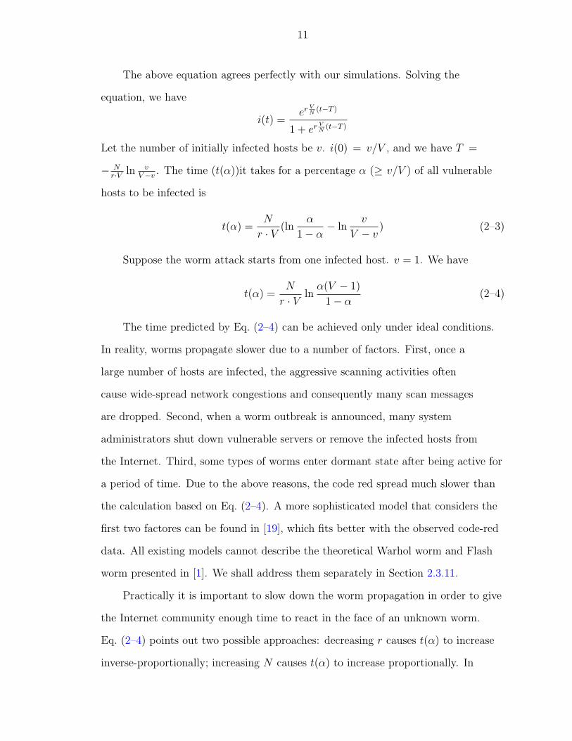
The time predicted by Eq. (2–4) can be achieved only under ideal conditions.
In reality, worms propagate slower due to a number of factors. First, once a
large number of hosts are infected, the aggressive scanning activities often
cause wide-spread network congestions and consequently many scan messages
are dropped. Second, when a worm outbreak is announced, many system
administrators shut down vulnerable servers or remove the infected hosts from
the Internet. Third, some types of worms enter dormant state after being active for
a period of time. Due to the above reasons, the code red spread much slower than
the calculation based on Eq. (2–4). A more sophisticated model that considers the
first two factores can be found in [19], which fits better with the observed code-red
data. All existing models cannot describe the theoretical Warhol worm and Flash
worm presented in [1]. We shall address them separately in Section 2.3.11.
Practically it is important to slow down the worm propagation in order to give
the Internet community enough time to react in the face of an unknown worm.
Eq. (2–4) points out two possible approaches: decreasing r causes t(α) to increase
inverse-proportionally; increasing N causes t(α) to increase proportionally. In
12
this paper, we use the first approach to slow down the worms, while relying on a
different technique to halt the propagation. The idea is to block out the infected
hosts and make sure that the scanning activity of an infected host does not last
for more than a period of ∆T . Under such a constraint, the propagation model
becomes
di(t)
dt= r
V
N(i(t)− i(t−∆T ))(1− i(t)) (2–5)
The above equation can be derived by following the same procedure that derives
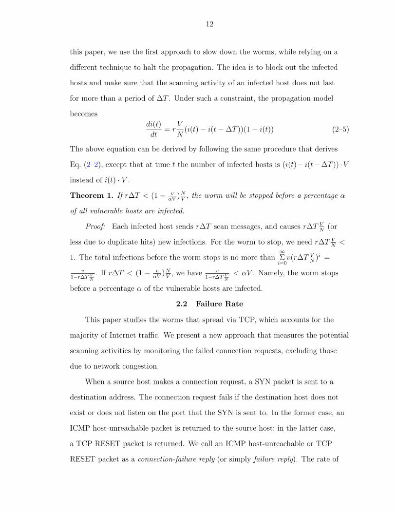
Eq. (2–2), except that at time t the number of infected hosts is (i(t)− i(t−∆T )) ·Vinstead of i(t) · V .
Theorem 1. If r∆T < (1 − vαV
)NV
, the worm will be stopped before a percentage α
of all vulnerable hosts are infected.
Proof: Each infected host sends r∆T scan messages, and causes r∆T VN
(or
less due to duplicate hits) new infections. For the worm to stop, we need r∆T VN
<
1. The total infections before the worm stops is no more than∞Σi=0
v(r∆T VN
)i =
v1−r∆T V
N
. If r∆T < (1 − vαV
)NV
, we have v1−r∆T V
N
< αV . Namely, the worm stops
before a percentage α of the vulnerable hosts are infected.
2.2 Failure Rate
This paper studies the worms that spread via TCP, which accounts for the
majority of Internet traffic. We present a new approach that measures the potential
scanning activities by monitoring the failed connection requests, excluding those
due to network congestion.
When a source host makes a connection request, a SYN packet is sent to a
destination address. The connection request fails if the destination host does not
exist or does not listen on the port that the SYN is sent to. In the former case, an
ICMP host-unreachable packet is returned to the source host; in the latter case,
a TCP RESET packet is returned. We call an ICMP host-unreachable or TCP
RESET packet as a connection-failure reply (or simply failure reply). The rate of

13
failed connection requests from a host s is called the failure rate, which can be
measured by monitoring the failure replys that are sent to s.
To support DAW, the ISP requires its customer networks to return ICMP
host-unreachable packets if the SYN packets are dropped by their routers or
firewalls. It is a common practice on the Internet.
It should be noted that our defense system does not require every customer
network that blocks ICMP to forward the log messages, although doing so helps
the performance of the system. Our defense system works well as long as a portion
(e.g., 10%) of all customer networks does not block ICMP host-unreachable
packets.
The failure rate measured for a normal host is likely to be low. For most
Internet applications (www, telnet, ftp, etc.), a user normally types domain names
instead of raw IP addresses to identify the servers. Domain names are resolved by
Domain Name System (DNS) for IP addresses. If DNS can not find the address
of a given name, the application will not issue a connection request. Hence,
mistyping or stale web links do not result in failed connection requests. An ICMP
host-unreachable packet is returned only when the server is off-line or the DNS
record is stale, which are both uncommon for popular or regularly-maintained
sites (e.g., Yahoo, Ebay, CNN, universities, governments, enterprises, etc.) that
attract most of Internet traffic. Moreover, a frequent user typically has a list of
favorite sites (servers) to which most connections are made. Since those sites
are known to work most of the time, the failure rate for such a user is likely to
be low. If a connection fails due to network congestion, it does not affect the
measurement of the failure rate because no ICMP host-unreachable or RESET
packet is returned. To illustrate our argument, we measured the failure rates on
three different domains of the University of Florida network. In our experiments,
domain 1 consists of five Class C networks, domain 2 consists of one Class C

14
avg. daily failure rate worst daily failure rate daily failure rateper host per host of the whole network
Domain 1 3.0 43 824Domain 2 10.1 41 116Domain 3 3.11 63 106
Table 2–1. Failure rates of normal hosts
network, and domain 2 consists of two Class C network. Table 2–1 clearly shows
that failure rates for normal hosts are typically very low.
On the other hand, the failure rate measured for a worm-infected host is likely
to be high. Unlike normal traffic, most connection requests initiated by a worm
fail because the destination addresses are randomly picked, which are likely either
not in use or not listening on the port that the worm targets at. Consider the
infamous code-red worm. Our experiment shows that 99.96% of all connections
made to random addresses at TCP port 80 fails. That is, the failure rate is 99.96%
of the scanning rate. For worms targeting at software that is less popular than
web servers, this figure will be even higher. The relation between the scanning rate
rsand the failure rate rfof a worm is
rf = (1− V ′
N)rs
where V ′is the number of hosts that listen on the attacked port(s).2 If V ′ << N ,
we have
rf ≈ rs (2–6)
Hence, measuring the failure rate of a worm gives a good idea about its scanning
rate. Given the aggressive behavior of a worm-infected host, its failure rate is
likely to be high, which sets it apart from the normal hosts. More importantly, an
2 V ≤ V ′ because not every host listens on the attacked port(s) is vulnerable.

15
approach that restricts the failure rate will restrict the scanning rate, which slows
down the worm propagation.
A worm may be deliberately designed to have a slow propagation rate in order
to evade the detection, which will be addressed in Section 2.3.9.
2.3 A Distributed Anti-Worm Architecture
2.3.1 Objectives
This section presents a distributed anti-worm architecture (DAW), whose main
objectives are
• Slowing down the worm propagation to allow human reaction time. It took
the code red just hours to achieve wide infection. Our goal is to prolong
that time to tens of days. A worm may even be stopped, especially when the
infected hosts scan at high rates, a property common to most known worms.
• Detecting potential worm activities and identifying likely offending hosts,
which provides the security management team with valuable information in
analyzing and countering the worm threat.
• Minimizing the performance impact on normal hosts and routers. Particularly,
a normal host should be able to make successful connections at any rate; a
server should be able to accept connections at any rate; the processing and
storage requirements on a router should be minimized.
2.3.2 Assumptions
Most businesses, institutions, and homes access the Internet via Internet
service providers (ISPs). An ISP network interconnects its customer networks,
and routes the IP traffic between them. The purpose of DAW is to provide an
ISP-based anti-worm service that prevents Internet worms from spreading among
the customer networks. DAW is practically feasible because its implementation
is within a single administrative domain. It also has strong business merit since

16
Internet Service Providercustomernetwork
customernetwork
edge routerswith DAW agent
neighbor ISP
management station
Figure 2–1. Distributed anti-worm Architecture
a large ISP has sufficient incentive to deploy such a system in order to gain
marketing edge against its competitors.
We assume that a significant portion of failure replys are not blocked within
the ISP. If the ISP address space is densely populated, then it is required that a
significant portion of TCP RESET packets are not blocked, which is normally the
case. If the ISP address space is sparsely populated, then it is required that ICMP
host-unreachable packets from a significant portion of addresses are not blocked,
which can be easily satisfied. Because there are many unused addresses, the ISP
routers will generate ICMP host-unreachable for those addresses. Hence, the ISP
simply has to make sure its own routers do not filter ICMP host-unreachable until
they are counted.
If some customer networks block all incoming SYN packets except for a list of
servers, their filtering routers should either generate ICMP host-unreachable for the
dropped SYN packets or, in case that ICMP replys are desirable, send log messages
to an ISP log station. Upon receipt of a log message, the log station sends an
ICMP host-unreachable towards the sender of the SYN packet. When an ISP edge
router receives an ICPM host-unreachable packet from the log station, it counts a
connection failure and drops the packet.

17
2.3.3 DAW Overview
As illustrated in Figure 2–1, DAW consists of two software components:
a DAW agent that is deployed on all edge routers of the ISP and a management
station that collects data from the agents. Each agent monitors the connection-failure
replys sent to the customer network that the edge router connects to. It identifies
the potential offending hosts and measures their failure rates. If the failure rate of
a host exceeds a pre-configured threshold, the agent randomly drops a minimum
number of connection requests from that host in order to keep its failure rate under
the threshold. A temporal rate-limit algorithm and a spatial rate-limit algorithm
are used to constrain any worm activity to a low level over the long term, while
accommodating the temporary aggressive behavior of normal hosts. Each agent
periodically reports the observed scanning activity and the potential offenders
to the management station. A continuous, steady increase in the gross scanning
activity raises the flag of a possible worm attack. The worm propagation is further
slowed or even stopped by blocking the hosts with persistently high failure rates.
Each edge router reads a configuration file from the management station about
what source addresses S and what destination ports P that it should monitor and
regulate. S consists of all or some addresses belonging to the customer network.
It provides a means to exempt certain addresses from DAW for research or other
purposes. P consists of the port numbers to be protected such as 80/8080 for
www, 23 for telnet, and 21 for ftp. It should exclude the applications that are not
suitable for DAW; for example, a hypothetical application runs with an extremely
high failure rate, making normal hosts undistinguishable from worms targeting
at the application. While DAW is not designed for all services, it is particularly
effective in protecting the services whose clients involve human interactions such
as web browsering, which makes greater distinction between normal hosts and
worm-infected hosts.

18
Throughout the paper, when we say “a router receives a connection request”,
we refer to a connection request that enters the ISP from a customer network, with
a source address in S and a destination port in P . When we say “a router receives
a failure reply”, we refer to a failure reply that leaves the ISP to a customer
network, with a destination address in S and a source port in P if it is a TCP
RESET packet.
This dissertation does not address the worm activity within a customer
network. A worm-infected host is not restricted in any way to infect other
vulnerable hosts of the same customer network. DAW works only against the
inter-network infections. The scanning rate of an infected host s is defined as the
number of connection requests sent by s per unit of time to addresses outside of the
customer network where s resides.
If a customer network has m(> 1) edge routers with the same ISP, the DAW
agent should be stalled on all m edge routers. If some edge routers are with
different ISPs that do not implement DAW, the network can be infected via those
ISPs but then are restricted in spreading the worm to the customer networks of the
ISPs that do implement DAW. For the purpose of simplicity, we do not consider
multi-homed networks in the analysis.
Based on the data from all agents, the controller monitors the total number
of potential offenders. A steady increase in the number of potential offenders
is considered as possible on-going worm propagation. When this happens,
the controller instructs the edge routers to block out a percentage of potential
offenders (i.e., their IP addresses) that have the highest failure rates. The controller
continues to double the percentage after each period (e.g., one minute) until
the number of potential offenders stops to increase. The reason to block only a
percentage instead of all potential offenders is as follows: the failure rates of some
normal hosts may happen to exceed the threshold amidst a worm attack. With a

19
mix of normal hosts and infected hosts, the aggressive behavior of worms makes
the infected hosts more likely to be blocked, while the normal hosts with marginal
exceeding failure rates remain unblocked.
On the other hand, if a normal host happens to run an automatic host-map
tool in the middle of a worm attack, it may be blocked due to high failure rate
of scanning activity. To prevent it from being blocked indefinitely, each blocked
address should be unblocked after certain period of time. An edge router keeps
a log of the blocked addresses and the number of times they are blocked recently
(e.g., during the past month). When an address is repetitively blocked, the
blocking time grows expontentially by T = T0ek, where T0 is the initial blocking
time and k is the number of prior blocks.
• How to monitor failed connection attempts? The answer to this question
allows DAW to separate the worm activity from most normal traffic and
consequently reduces the amount of information that DAW has to process.
• How to achieve bounded failure rate? The answer to this question effectively
limits the maximum scanning rate (r in Eq. (2–4)) of any infected host.
• How to reduce false positives? The answer to this question helps to reduce
the impact on normal hosts.
• How to automatically generate the worm signatures? The answer to this
question allows DAW to work with intrusion-detection devices and firewalls to
identify and filter out the worm traffic.
2.3.4 Measuring Failure Rate
Each edge router measures the failure rates for the addresses belonging to the
customer network that the router connects to.
A failure-rate record consists of an address field s, a failure rate field f ,
a timestamp field t, and a failure counter field c. The initial values of f and c
are zeros; the initial value of t is the system clock when the record is created.
20
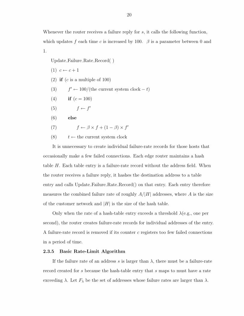
Whenever the router receives a failure reply for s, it calls the following function,
which updates f each time c is increased by 100. β is a parameter between 0 and
1.
Update Failure Rate Record( )
(1) c ← c + 1
(2) if (c is a multiple of 100)
(3) f ′ ← 100/(the current system clock− t)
(4) if (c = 100)
(5) f ← f ′
(6) else
(7) f ← β × f + (1− β)× f ′
(8) t ← the current system clock
It is unnecessary to create individual failure-rate records for those hosts that
occasionally make a few failed connections. Each edge router maintains a hash
table H. Each table entry is a failure-rate record without the address field. When
the router receives a failure reply, it hashes the destination address to a table
entry and calls Update Failure Rate Record() on that entry. Each entry therefore
measures the combined failure rate of roughly A/|H| addresses, where A is the size
of the customer network and |H| is the size of the hash table.
Only when the rate of a hash-table entry exceeds a threshold λ(e.g., one per
second), the router creates failure-rate records for individual addresses of the entry.
A failure-rate record is removed if its counter c registers too few failed connections
in a period of time.
2.3.5 Basic Rate-Limit Algorithm
If the failure rate of an address s is larger than λ, there must be a failure-rate
record created for s because the hash-table entry that s maps to must have a rate
exceeding λ. Let Fλ be the set of addresses whose failure rates are larger than λ.

21
For each s ∈ Fλ, the router reduces its failure rate below λ by rate-limiting the
connection requests from s. A token bucket is used. Let size be the bucket size,
tokens be the number of tokens, and time be a timestamp whose initial value is the
system clock when the algorithm starts.
Upon receipt of a failure reply to s
(1) tokens ← tokens− 1
Upon receipt of a connection request from s
(2) ∆t ← the current system clock− time
(3) tokens ← mintokens + ∆t× λ, size(4) time ← the current system clock
(5) if (tokens ≥ 1)
(6) forward the request
(7) else
(8) drop the request
It should be emphasized that the above algorithm is not a traditional
token-bucket algorithm that buffers the oversized bursts and releases them at
a fixed average rate. The purpose of our algorithm is not to shape the flow of
incoming failure replys but to shape the “creation” of the failure replys. It ensures
that the failure rate of any address in S stays below λ. This effectively restricts the
scanning rate of any worm-infected host (Eq. 2–6).
This and other rate-limit algorithms are performed on individual addresses.
They are not performed on the failure-rate records in the hash table; that is
because otherwise many addresses would have been blocked due to one scan source
mapped to the same hash-table entry.
One fundamental idea of DAW is to make the speed of worm propagation
no longer determined by the worm parameters set by the attackers, but by the

22
DAW parameters set by the ISP administrators. In the following, we propose more
advanced rate-limit algorithms to give the defenders greater control.
2.3.6 Temporal Rate-Limit Algorithm
A normal user behaves differently from a worm that scans the Internet
tirelessly, day and night. A user may generate a failure rate close to λ for a
short period of time, but that can not last for every minute in 24 hours of a
day. While we set λ large enough to accommodate temporary aggressiveness in
normal behavior, the rate over a long period can be tightened. Let Ωbe the system
parameter that controls the maximum number of failed connection requests allowed
for an address per day. Let D be the time of a day. Ω can be set much smaller
than λD.
At the start of each day, the counters (c) of all failure-rate records and
hash-table entries are reset to zeros. The value of c always equals the number of
failed requests that have happened during the day. A hash-table entry creates
failure-rate records for individual addresses when either f > λ or c > Ω.
A temporal rate-limit algorithm is designed to bound the maximum number of
failed requests per day. Let FΩ be the set of addresses with individual failure-rate
records and ∀s ∈ FΩ, either the failure rate of s is larger than λ or the counter of s
reaches Ω/2. It is obvious that Fλ ⊆ FΩ.
Upon receipt of a failure reply to s
(1) tokens ← tokens− 1
Upon receipt of a connection request from s
(2) ∆t ← the current system clock− time
(3) if (c ≤ Ω/2)
(4) tokens ← mintokens + ∆t× λ, size(5) else
23
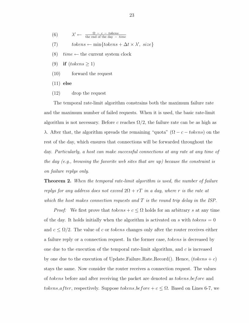
(6) λ′ ← Ω − c − tokensthe end of the day − time
(7) tokens ← mintokens + ∆t× λ′, size(8) time ← the current system clock
(9) if (tokens ≥ 1)
(10) forward the request
(11) else
(12) drop the request
The temporal rate-limit algorithm constrains both the maximum failure rate
and the maximum number of failed requests. When it is used, the basic rate-limit
algorithm is not necessary. Before c reaches Ω/2, the failure rate can be as high as
λ. After that, the algorithm spreads the remaining “quota” (Ω− c− tokens) on the
rest of the day, which ensures that connections will be forwarded throughout the
day. Particularly, a host can make successful connections at any rate at any time of
the day (e.g., browsing the favorite web sites that are up) because the constraint is
on failure replys only.
Theorem 2. When the temporal rate-limit algorithm is used, the number of failure
replys for any address does not exceed 2Ω + rT in a day, where r is the rate at
which the host makes connection requests and T is the round trip delay in the ISP.
Proof: We first prove that tokens + c ≤ Ω holds for an arbitrary s at any time
of the day. It holds initially when the algorithm is activated on s with tokens = 0
and c ≤ Ω/2. The value of c or tokens changes only after the router receives either
a failure reply or a connection request. In the former case, tokens is decreased by
one due to the execution of the temporal rate-limit algorithm, and c is increased
by one due to the execution of Update Failure Rate Record(). Hence, (tokens + c)
stays the same. Now consider the router receives a connection request. The values
of tokens before and after receiving the packet are denoted as tokens before and
tokens after, respectively. Suppose tokens before + c ≤ Ω. Based on Lines 6-7, we
24
have
tokens after
= mintokens before + ∆t× λ′, size
≤ tokens before + ∆t× Ω − c − tokens before
the end of the day − time
≤ tokens before + (Ω− c− tokens before)
≤ Ω− cTherefore, tokens after + c ≤ Ω.
Next we prove that tokens ≥ −rT at the end of the day. Consider the
case that tokens < 1 at the end of the day. Without losing generality, suppose
tokens ≥ 1 before time t0, 0 ≤ tokens < 1 after t0 due to the execution of Line 1,
and then tokens stays less than one for the rest of the day. After t0, all connection
requests from s are blocked (Line 12). For all requests sent before t0−T , the failure
replys must have already arrived before t0. There are at most rT requests sent
between t0 − T and t0. Therefore, there are at most rT failure replys arriving after
t0. We know that tokens ≥ 0 at t0. Hence, tokens ≥ −rT at the end of the day.
Because tokens + c ≤ Ω holds at any time, c ≤ Ω + rT at the end of the day.
The counter c equals the number of failure replys received during the day after
the failure-rate record for s is created. Before that, there are at most Ω failure
replys counted by the hash-table entry that s maps to. In the worst case all those
replys are for s. Therefore, the total number of failure replys for s is no more than
2Ω + rT .
rT is normally small because the typical round trip delay across the Internet
is in tens or hundreds of milliseconds. Hence, if Ω = 300, the average scanning
rate of a worm is effectively limited to about 2Ω/D = 0.42/min. In comparison,
Williamson’s experiment showed that the scanning rate of the code red was at least
200 / second [12], which is more than 28,000 times faster. Yet, it took the code red

25
hours to spread, suggesting the promising potential of using the temporal rate-limit
algorithm to slow down worms.
Additional system parameters that specify the maximum numbers of failed
requests in longer time scales (week or month) can further increase the worm
propagation time.
2.3.7 Recently Failed Address List
If a major web server such as Yahoo or CNN is down, an edge router may
observe a significant surge in failure replys even though there is no worm activity.
To solve this problem, each edge router maintains a recently failed address list
(RFAL), which is emptied at the beginning of each day. When the router receives
a failure reply from address d, it matches d against the addresses in RFAL. If d
is in the list, the router skips all DAW-related processing. Otherwise, it inserts d
into RFAL before processing the failure reply. If RFAL is full, d replaces the oldest
entry in the list.
When a popular server is down, if it is frequently accessed by the hosts in
the customer network, the server’s address is likely to be in RFAL and the failure
replys from the server will not be repetitively counted. Hence, the number of
failed requests allowed for a normal host per day can be much larger than Ω. It
effectively places no restriction on keeping trying a number of favorite sites that are
temporarily down. On the other hand, given the limited size of RFAL (e.g., 1000)
and the much larger space of IPv4 (232), the random addresses picked by worms
have a negligibly small chance to fall in the list.
2.3.8 Spatial Rate-Limit Algorithm
While each infected host is regulated by the temporal rate-limit algorithm,
there may be many of them, whose aggregated scanning rate can be very high.
DAW uses a spatial rate-limit algorithm to constrain the combined scanning rate
of infected hosts in a customer network. Let Φbe the system parameter that

26
controls the total number of failed requests allowed for a customer network per
day. It may vary for different customer networks based on their sizes. Once the
number of addresses inserted to RFAL exceeds Φ, the system starts to create
failure-rate records for all addresses that receive failure replys, and activates
the spatial algorithm. If there are too many records, it retains those with the
largest counters. Let FΦ (∈ S) be the set of addresses whose counters exceed a
small threshold τ (e.g., 50), which excludes the obvious normal hosts. The spatial
rate-limit algorithm is the same as the temporal algorithm except that s, Ω, and
c are replaced respectively by FΦ, Φ, and the total number of failure replys to FΦ
received after the spatial algoirthm is activiated.
For any address s in FΩ ∩ FΦ, the temporal rate-limit algorithm is first
executed and then the spatial rate-limit algorithm is executed. The reason to
apply the temporal algorithm is to prevent a few aggressive infected hosts from
keeping reducing tokens to zero. On the other hand, if there are a large number
of infected hosts, causing the spatial algorithm to drop most requests, the router
should temporarily block the addresses whose failure-rate records have the largest
counters.
The edge routers may be configured independently with some running both
the temporal and spatial algorithms but some running the temporal algorithm only.
For example, the edge routers for the neighbor ISPs should have large Φ values or
not run the spatial algorithm.
Theorem 3. When the spatial rate-limit algorithm is used, the total number of
failure replys per day for all infected hosts in a customer network is bounded by
2Φ + mr′T , where m is the number of addresses in FΦ, r′ is the scanning rate of an
infected host after the temporal rate-limit algorithm is applied, and T is the round
trip delay of the ISP.

27
Due to space limitation, the proof is omitted, which is very similar to the proof
for Theorem 2. mr′T is likely to be small because both r′ and T are small.
The following analysis is based on a simplified model. A more general model
will be used in the simulations. Suppose there are k customer networks, each with
V/k vulnerable hosts. Once a vulnerable host is infected, we assume all other
vulnerable hosts in the same customer networks are infected immediately because
DAW does not restrict the scanning activity within the customer network. Based
on Theorem 3, the combined scanning rate of all vulnerable hosts in a customer
network is (2Φ + mrT )/D ≈ 2Φ/D. Let j(t) be the percentage of customer
networks that are infected by the worm.
At time t, the number of infected customer networks is j(t) · k, and the number
of uninfected networks is (1 − j(t))k. The probability for one scan message to hit
an uninfected vulnerable host and thus infect the network where the host resides
is (1 − j(t))V/N . For an infinitely small period dt, j(t) changes by dj(t). During
that time, there are 2ΦD· j(t) · k · dt scan messages and the number of newly infected
networks is 2ΦD· j(t) · k · dt · (1− j(t))V/N = 2Φ
D· j(t) · (1− j(t))V k
Ndt. 3 Therefore,
k · dj(t) =2Φ
D· j(t) · (1− j(t))
V k
Ndt
dj(t)
dt=
2V Φ
NDj(t)(1− j(t))
j(t) =e
2V ΦND
(t−T )
1 + e2V ΦND
(t−T )
Assume there is one infection at time 0. We have T = − ND2V Φ
ln 1k−1
. The time it
takes to infect α percent of all networks is
t(α) =ND
2 · V Φln
α(k − 1)
1− α
3 The probability of multiple external infections of the same network is negligiblewhen dt → 0.

28
Suppose an ISP wants to ensure that the time for α percent of networks to be
infected is at least γ days. The value of Φ should satisfy the following condition.
Φ ≤ N
2 · V γln
α(k − 1)
1− α
which is not related to how the worm behaves.
2.3.9 Blocking Persistent Scanning Sources
The edge routers are configured to block out the addresses whose counters
(c) reach Ω for n consecutive days, where n is a system parameter. If the
worm-infected hosts perform high-speed scanning, they will each be blocked
out after n days of activity. Hence the worm propagation may be stopped before an
epidemic materializes, according to Eq. (2–5).
The worm propagates slowly under the temporal rate-limit algorithm and the
spatial rate-limit algorithm. It gives the administrators sufficient time to study the
traffic of the hosts to be blocked, perform analysis to determine whether a worm
infection has occurred, and decide whether to approve or disapprove the blocking.
Once the threat of a worm is confirmed, the edge routers may be instructed to
reduce n, which increases the chance of fully stopping the worm.
Suppose a worm scans more than Ω addresses per day. The worm propagation
can be completely stopped if each infected customer network makes less than one
new infection on average before its infected hosts are blocked. The number of
addresses scanned by the infected hosts from a single network during n days is
about 2nΦ by Theorem 3. Each message has a maximum probability of V/N to
infect a new host. Hence, the condition to stop a worm is
2nΦV
N< 1

29
The expected total number of infected networks is bounded by
∞Σi=0
(2nΦV
N)i =
1
1− 2nΦ VN
On the other hand, when 2nΦ VN≥ 1, the worm may not be stopped by the above
approach alone. However the significance of blocking infected hosts should not be
under-estimated as it makes the worm-propagation time longer and gives human or
other automatic tools (e.g., the one described below) more reaction time.
If the scanning rate of a worm is below Ω per day, the infected hosts will not
be blocked. DAW relys on a different approach to address this problem. During
each day, an edge router e measures the total number of connection requests,
denoted as nc(e), and the total number of failure replys, denoted as nf (e). Note
that only the requests and replys that match S and P (Section 2.3.3) are measured.
The router sends these numbers to the management station at the end of the day.
The management station measures the following ratio
Σe∈E
nf (e)
Σe∈E
nc(e)
where E is the set of edge routers. If the ratio increases significantly for a number
of days, it signals a potential worm threat. That is because the increase in failed
requests steadily outpaces the increase in issued requests, which is possibly the
result of more and more hosts being infected by worms.
The management station then instructs the edge routers to identify potential
offenders whose counters (c) have the highest values. Additional potential offenders
are found as follows. After a vulnerable server is infected via a port that it listens
to, the server normally scans the Internet on the same port to infect other servers.
Based on this observation, when an edge router receives a RESET packet with a
source address d, a source port p ∈ P to a destination address s ∈ S, it sends a
SYN packet to check if s is also listening on port p. If it is, the router marks s as a

30
potential offender and creates a failure-rate record, which measures the number of
failed connections from s. At the end of each day, the management station collects
the potential offenders from all edge routers. Those with the largest counters are
presented to the administrators for traffic analysis. The management station may
instruct the edge routers to block them if the worm threat is confirmed.
Although a blocked server can not issue connection requests before it is
unblocked, it can accept connection requests at any rate. Its role of a server is
unchanged. An alternative to complete blocking is to apply a different, small Ω
value (e.g., 50) on those addresses, which leaves room for false positives since the
hosts can still make as many successful connections as they want, with occasional
failures.
2.3.10 FailLog
For a customer that blocks all ICMP traffic,4 its routers/firewalls should be
configured to send a log message to the local management station when a packet is
dropped, which is today’s common practice. If the dropped packet is a SYN packet,
the management station forwards a copy of the log message to the nearest ISP edge
router, which in turn encapsulates the log in a control message (called FailLog) and
sends the message to the source address s of the SYN. The FailLog is then routed
across the ISP network to the edge router of s. An edge router is reponsible of
measuring the failure rates for the addresses in the customer network it connects
to. Upon receipt of the FailLog, the edge router updates the failure rate of s and
discard the message.
The failure rate of a source address is the combined rate of RESET, ICMP
host-unreachable, and FailLog messages that are sent to the address. The
4 It is common for an organization to block all inbound ICMP requests but notcommon to block all inbound/outbound ICMP traffic.

31
requirement for customer networks that block ICMP to generate FailLog will
be relaxed in Section 2.3.10.
It has been assumed so far that every customer network that blocks ICMP
will generate FailLog messages. We now relax this requirement. Consider a worm
that targets at one or multiple ports (e.g, web service). Let A be the IP address
space that are not occupied by the hosts listening on those ports. Let p1 be the
percentage of A that is used by existing hosts. Let p2 be the percentage of A that
is not used but reponds connection requests with ICMP host-unreachable packets
(generated by routers). This includes the ISP’s reserved addresses for future
expansion. Let p3 be the percentage of A that is not used and does not repond
with ICMP host-unreachable packets. Among p3, Let p′3 be the percentage that
generates FailLog. p1 + p2 + p3 = 1 and 0 ≤ p′3 ≤ p3.
Eq. (2–6) was derived under the condition that p′3 = p3. If none or only some
customer networks generate FailLog, the equation becomes
rs ≈ 1
p1 + p2 + p′3rf
For example, if p1 = 10%, p2 = 60% and p′3 = 0%, 5 then the scanning rate of any
worm-infected host will be roughly 1.4 times of the failure rate controlled by λ and
Ω. Our simulation shows that DAW works well even when p1 + p2 + p′3 = 10%.
The actual value of p1 + p2 + p′3 can be measured by the management
station by generating connection requests to random addresses and monitoring the
connection-failure replys. Since rs is known and rf can be measured, p1 + p2 + p′3 =
rf/rs. Note that the scanning rate of the management station is not constrained by
DAW because it is inside the ISP network.
5 This is a conservation assumption because firewalls are often configured toblock ICMP requests but not ICMP host-unreachable replys.

32
2.3.11 Warhol Worm and Flash Worm
The Warhol worm and the Flash worm are hypothetical worms studied in [1],
which embodied a number of highly effective techniques that the future worms
might use to infect the Internet in a very short period of time, leaving no room for
human actions.
In order to improve the chance of infection during the initial phase, the Warhol
worm first scans a pre-made list of (e.g., 10000 to 50000) potentially vulnerable
hosts, which is called a hit-list. After that, the worm performs permutation
scanning, which divides the address space to be scanned among the infected hosts.
One way to generate a hit-list is to perform a scan of the Internet before the worm
is released [1]. With DAW, it will take about N/2Ω days. Suppose Ω = 300 and
N = 232. That would be 19611 years. Even if the hit-list can be generated by
a different means, the permutation scanning is less effective under DAW. For
instance, even after 10000 vulnerable hosts are infected, they can only probe about
10000 × 2Ω = 6 × 10⁶ addresses a day. Considering the size of the address space is
232 ≈ 4.3 × 10⁹, duplicate hits are not a serious problem, which means the gain by
permutation scanning is small. Without DAW, it will be a different matter. If the
scanning rate is 200/second, it takes less than 36 minutes for 10000 infected hosts
to make 232 probes, and duplicate hits are very frequent.
The Flash worm assumes a hit-list L including most servers that listen on
the targeted port. Hence, random scanning is completely avoided; the worm scans
only the addresses in L. As more and more hosts are infected, L is recursively split
among the newly infected hosts, which scan only the assigned addresses from L.
The Flash worm requires a prescan of the entire Internet before it is released. Such
a prescan takes too long under DAW. In addition, each infected host can only scan
about 2Ω addresses per day, which limits the propagation speed of the worm if L is
large.
33
0
0.2
0.4
0.6
0.8
1
0 2 4 6 8 10 12 14 16 18
i(t)
t (hours)
No AlgorithmBasic Rate-Limit
TemporalTemporal + Spatial
DAW
0
0.2
0.4
0.6
0.8
1
0 20 40 60 80 100
i(t)
t (days)
No AlgorithmBasic Rate-Limit
TemporalTemporal + Spatial
DAW
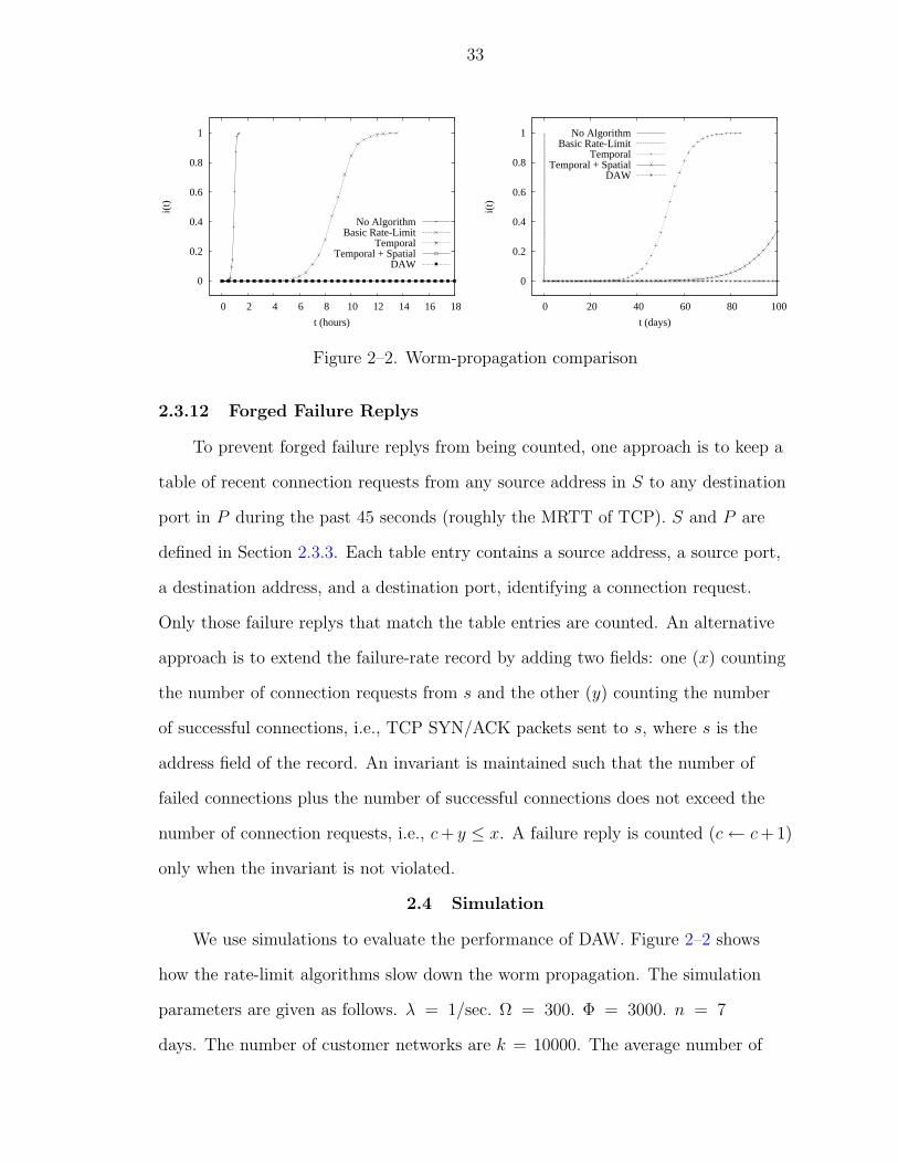
Figure 2–2. Worm-propagation comparison
2.3.12 Forged Failure Replys
To prevent forged failure replys from being counted, one approach is to keep a
table of recent connection requests from any source address in S to any destination
port in P during the past 45 seconds (roughly the MRTT of TCP). S and P are
defined in Section 2.3.3. Each table entry contains a source address, a source port,
a destination address, and a destination port, identifying a connection request.
Only those failure replys that match the table entries are counted. An alternative
approach is to extend the failure-rate record by adding two fields: one (x) counting
the number of connection requests from s and the other (y) counting the number
of successful connections, i.e., TCP SYN/ACK packets sent to s, where s is the
address field of the record. An invariant is maintained such that the number of
failed connections plus the number of successful connections does not exceed the
number of connection requests, i.e., c + y ≤ x. A failure reply is counted (c ← c + 1)
only when the invariant is not violated.
2.4 Simulation
We use simulations to evaluate the performance of DAW. Figure 2–2 shows
how the rate-limit algorithms slow down the worm propagation. The simulation
parameters are given as follows. λ = 1/sec. Ω = 300. Φ = 3000. n = 7
days. The number of customer networks are k = 10000. The average number of

34
vulnerable hosts per customer network is z = 10. The numbers of vulnerable hosts
in different customer networks follow an exponential distribution, suggesting a
scenario where most customer networks have ten or less public servers, but some
have large numbers of servers. Suppose the worm uses a Nimda-like algorithm that
aggressively searches the local-address space. We assume that once a vulnerable
host of a customer network is infected, all vulnerable hosts of the same network are
infected shortly.
Figure 2–2 compares the percentage i(t) of vulnerable hosts that are infected
over time t in five different cases: 1) no algorithm is used, 2) the basic rate-limit
algorithm is implemented on the edge routers, 3) the temporal rate-limit algorithm
is implemented, 4) both the temporal and spatial rate-limit algorithms are
implemented, or 5) DAW (i.e., Temporal, Spatial, and blocking persistent scanning
sources) is implemented. Note that all algorithms limit the failure rates, not
the request rates, and the spatial rate-limit algorithm is applied only on the
hosts whose failure counters exceed a threshold τ = 50. Two graphs show the
simulation results in different time scales. The upper graph is from 0 to 18 hours,
and the lower is from 0 to 100 days. The shape of the curve “No Algorithm”
depends on the worm’s scanning rate, which is 10/sec in our simulation. The other
four curves are independent of the worm’s scanning rate; they depend only on
DAW’s parameters, i.e., λ, Ω, Φ, and n. The figure shows that the basic rate-limit
algorithm slows down the worm propagation from minutes to hours, while the
temporal rate-limit algorithm slows down the propagation to tens of days. The
spatial rate-limit algorithm makes further improvement on top of that — it takes
the worm 80 days to infect 5% of the vulnerable hosts, leaving sufficient time for
human intervention. Moreover, with persistent scanning sources being blocked after
7 days, DAW is able to stop the worm propagation at i(t) = 0.000034.

35
k z Ω = 1000 = 3000 = 5000 = 70005000 10 350.3 116.8 69.6 50.25000 20 237.2 79.1 47.2 33.910000 10 190.1 63.5 38.1 27.110000 20 127.9 42.5 25.5 18.315000 10 133.6 44.4 26.3 19.315000 20 89.3 29.7 17.8 12.720000 10 103.3 34.2 20.6 14.620000 20 68.9 22.9 13.8 10.0
Table 2–2. 5% propagtion time (days) for “Temporal + Spatial”
Table 2–2 shows the time it takes the worm to infect 5% of vulnerable hosts
(called 5% propagation time) under various conditions with Temporal + Spatial
implemented. Depending on the size (k and z) of the ISP, the propagation time
ranges from 10.0 days to 350.3 days. To ensure a large propagation time, a very
large ISP may partition its customers into multiple defense zones of modest sizes.
DAW can be implemented on the boundary of each zone, consisting of the edge
routers to the customer networks of the zone and the internal routers connecting to
other zones.
Figure 2–3 shows the performance of the temporal rate-limit algorithm with
respect to the parameter Ω. As expected, the propagation time decreases when Ω
increases. The algorithm performs very well for modest-size ISPs (or zones). When
k = 10000, z = 10 and Ω = 3000, the 5% propagation time is 63.6 days. Figure
2–4 shows the performance of the spatial rate-limit algorithm (alone) with respect
to the parameter Φ. The algorithm works well for modest-size ISPs (or zones) even
for large Φ values. When k = 10000, z = 10 and Φ = 7000, the 5% propagation
time is 27.2 days. The performance of the two algorithms is comparable when
Φ = z×Ω, where the total temporal rate limit of the local infected hosts is equal to
the spatial rate limit. As shown in the figures, if Φ > z ×Ω, the temporal algorithm
works better; if Φ < z × Ω, the spatial algorithm works better. Therefore, the two
algorithms are complementary to each other and they are both adopted by DAW.

36
0
50
100
150
200
250
300
350
0 100 200 300 400 500 600 700
5% p
ropa
gatio
n tim
e (d
ays)
Omega
k = 10,000 z = 5k = 10,000 z = 10k = 10,000 z = 20k = 20,000 z = 10k = 20,000 z = 20
Figure 2–3. Effectiveness of thetemporal rate-limitalgorithm for DAW
0
50
100
150
200
250
300
350
0 1000 2000 3000 4000 5000 6000 7000
5% p
ropa
gatio
n tim
e (d
ays)
Phi
k = 10,000 z = 5k = 10,000 z = 10k = 10,000 z = 20k = 20,000 z = 10k = 20,000 z = 20
Figure 2–4. Effectiveness of the spatialrate-limit algorithm forDAW
0
0.2
0.4
0.6
0.8
1
0 2 4 6 8 10
fina
l inf
ectio
n pe
rcen
tage
n (days)
k = 10,000 z = 5k = 10,000 z = 10k = 10,000 z = 20k = 20,000 z = 10k = 20,000 z = 20
Figure 2–5. Stop worm propagation byblocking
0
200
400
600
800
1000
0 2 4 6 8 10
tota
l pro
paga
tion
time
(day
s)
n (days)
k = 10,000 z = 5k = 10,000 z = 10k = 10,000 z = 20k = 20,000 z = 10k = 20,000 z = 20
Figure 2–6. Propagation time beforethe worm is stopped
Because DAW blocks persistent scanning sources, it may stop the worm
propagation, depending on the value of n. Figure 2–5 shows the final infection
percentage among the vulnerable hosts before all infected hosts are blocked. Even
when a large n is selected and the final infection percentage is large, the blocking is
still very useful because it considerably slows down the worm propagation as shown
in Figure 2–6, where only the propagation times for larger-than-5% final infections
are shown. For instance, when k = 20000, z = 20 and n = 10, the final infection
percentage is close to 100%. However, it will take the worm 71.7 days to achieve
that.

CHAPTER 3A SIGNATURE-BASED APPROACH
3.1 Double-Honeypot System
3.1.1 Motivation
The spread of a malicious worm is often an Internet-wide event. The
fundamental difficulty in detecting a previously unknown worm is due to two
reasons. First, the Internet consists of a large number of autonomous systems
that are managed independently, which means a coordinated defense system
covering the whole Internet is extremely difficult to realize. Second, it is hard to
distinguish the worm activities from the normal activities, especially during the
initial spreading phase. Although the worm activities become apparent after a
significant number of hosts are infected, it will be too late at that time due to the
exponential growth rate of a typical worm [19, 22, 21, 18, 17]. In contrast to some
existing defense systems that require large-scale coordinated efforts, we describe a
double-honeypot system that allows an individual autonomous system to detect the
ongoing worm threat without external assistance. Most importantly, the system is
able to detect new worms that are not seen before.
Before presenting the architecture of our double-honeypot system, we give a
brief introduction of honeypot. Developed in recent years, honeypot is a monitored
system on the Internet serving the purpose of attracting and trapping attackers
who attempt to penetrate the protected servers on a network [28]. Honeypots
fall into two categories [29] A high-interaction honeypot operates a real operating
system and one or multiple applications. A low-interaction honeypot simulates one
or multiple real systems. In general, any network activities observed at honeypots
are considered as suspicious and it is possible to capture the latest intrusions based
37
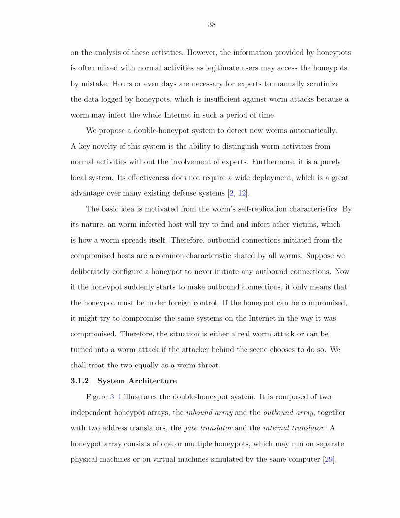
38
on the analysis of these activities. However, the information provided by honeypots
is often mixed with normal activities as legitimate users may access the honeypots
by mistake. Hours or even days are necessary for experts to manually scrutinize
the data logged by honeypots, which is insufficient against worm attacks because a
worm may infect the whole Internet in such a period of time.
We propose a double-honeypot system to detect new worms automatically.
A key novelty of this system is the ability to distinguish worm activities from
normal activities without the involvement of experts. Furthermore, it is a purely
local system. Its effectiveness does not require a wide deployment, which is a great
advantage over many existing defense systems [2, 12].
The basic idea is motivated from the worm’s self-replication characteristics. By
its nature, an worm infected host will try to find and infect other victims, which
is how a worm spreads itself. Therefore, outbound connections initiated from the
compromised hosts are a common characteristic shared by all worms. Suppose we
deliberately configure a honeypot to never initiate any outbound connections. Now
if the honeypot suddenly starts to make outbound connections, it only means that
the honeypot must be under foreign control. If the honeypot can be compromised,
it might try to compromise the same systems on the Internet in the way it was
compromised. Therefore, the situation is either a real worm attack or can be
turned into a worm attack if the attacker behind the scene chooses to do so. We
shall treat the two equally as a worm threat.
3.1.2 System Architecture
Figure 3–1 illustrates the double-honeypot system. It is composed of two
independent honeypot arrays, the inbound array and the outbound array, together
with two address translators, the gate translator and the internal translator. A
honeypot array consists of one or multiple honeypots, which may run on separate
physical machines or on virtual machines simulated by the same computer [29].

39
Internet
Gate Translater
Internal Translater
Honeypots
Worm
Inbound Array
Outbound Array
Honeypots
Local Network
Firewall
Signature Center
Figure 3–1. Using double-honeypot detecting Internet worms
Each honeypot in the array runs a server identical to a local server to be protected.
A honeypot in the inbound (outbound) array is called an inbound (outbound)
honeypot. Our goal is to attract a worm to compromise an inbound honeypot
before it compromises a local server. When the compromised inbound honeypot
attempts to attack other machines by making outbound connections, its traffic is
redirected to an outbound honeypot, which captures the attack traffic.
An inbound honeypot should be implemented as a high-interaction honeypot
that accepts connections from outside world in order to be compromised by
worms that may pose a threat to a local server. An outbound honeypot should be
implemented as a low-interaction honeypot so that it can remain uninfected when
it records the worm traffic. In addition to performing the functionalities of the local
system, it checks and records all network traffic in a connection initiated from an
inbound honeypot. The network traffic, which is directly related to worm activities
from the outside, will be analyzed to identify the signatures of the worms.
The gate translator is implemented at the edge router between the local
network and the Internet. It samples the unwanted inbound connections, and
redirects the sampled connections to inbound honeypots that run the server

40
software the connections attempt to access (e.g., connections to ports 80/8080
are redirected to a honeypot running a web server). There are several ways
to determine which connections are “unwanted”. The gate translator may be
configured with a list of unused addresses. Connections to those addresses are
deemed to be unwanted. It is very common nowadays for an organization to expose
only the addresses of its public servers. If that is the case, the gate translator can
be configured with those publicly-accessible addresses. When a connection for a
specific service (e.g., to port 80 for web access) is not made to one of the servers,
it is unwanted and redirected to an inbound honeypot. Suppose the size of the
local address space is Nand there are hpublicly-accessible servers on a particular
destination port. Typically, N >> h. For a worm which randomly scans that port,
the chance for it to hit an inbound honeypot first is N−hN
, and the chance for it to
hit a protected server first is hN
. With a ratio of N−hh
, it is almost certain that the
worm will compromise the inbound honeypot before it does any damage to a real
server within the network.
Once an inbound honeypot is compromised, it will attempt to make outbound
connections. The internal translator is implemented at a router that separates the
inbound array from the rest of the network. It intercepts all outbound connections
from an inbound honeypot and redirects them to an outbound honeypot of the
same type, which will record and analyze the traffic.
We give the following example to illustrate how the system works. Suppose
that the IP address space of our network is 128.10.10.0/128, with one public web
server Y to be protected. The server’s IP address is 128.10.10.1. Suppose an
attacker outside the network initiates a worm attack against systems of type Y .
The worm scans the IP address space for victims. It is highly probable that an
unused IP address, e.g. 128.10.10.20, will be attempted before 128.10.10.1. The
gate controller redirects the packets to an inbound honeypot of type Y , which is

41
subsequently infected. As the compromised honeypot participates in spreading the
worm, it will reveal itself by making outbound connections and provide the attack
traffic that will be redirected to an outbound honeypot of the system.
After an outbound honeypot captured a worm, the payload of the worm can
be directly considered as a signature. Using traffic filtering with the signature
at the edge of the network will protect the hosts from being attacked by the
same worm. In our system, the payload of the worm will also be forwarded to a
signature center. If a worm with polymorphism has been used during the attack,
the signature center will generate one single signature for all the variants of one
olymorphic worm by the algorithms discussed later. The special will not only be
able to match those variants whose payloads have been captured before, it can also
match those variants not seen before.
We should emphasis that, the proposed double-honeypot system is greatly
different from a conventional honeypot. A conventional system receives traffic from
all kinds of sources, including traffic from the normal users. It is a difficult and
tedious task to separate attack traffic from normal traffic, especially for attacks
that are not seen before. It is more than often that, only after the damage of the
new attacks is surfaced, the experts rush to search the recorded data for the trace
of attack traffic. In our system, when an outbound honeypot receives packets from
an inbound honeypot, it knows for sure that the packets are from a malicious
source. The outbound honeypot does not have to face the potentially huge amount
of normal background traffic that a conventional honeypot may receive.
3.2 Polymorphism of Internet Worms
The double-honeypot system provides a means to capture the byte sequences
of previous unknown Internet worms without manual analysis from the experts.
The captured byte sequences can be used to generate worm signatures, and future
connections carrying them will be automatically blocked. This is a great advantage

42
mov edi, 00403045h ; Set EDI to Start
add edi, ebp ; Adjust according to base
mov ecx, 0A6Bh ; length of encrypted virus body
mov al, [key] ; pick the key
Decrypt:
xor [edi], al ; decrypt body
inc edi ; increment counter position
loop Decrypt ; until all bytes are decrypted
jmp Start ; Jump to Start (jump over some data)
DB key 86 ; variable one byte key
Start: ; encrypted/decrypted virus body
Figure 3–2. A decryptor example of a worm.
over the current systems because the defense can be carried out automatically
before new worms deal a significant damage to the network.
The attackers will try every possible way to extend the life time of Internet
worms. In order to evade the signature-based system, a polymorphic worm appears
differently each time it replicates itself. This section discusses the polymorphism of
Internet worms, while the next section provides a solution against some common
polymorphism techniques.
There are many ways to make polymorphic worms. One technique relies on self
encryption with a variable key. It encrypts the body of a worm, which erases both
signatures and statistical characteristics of the worm byte string. A copy of the
worm, the decryption routine, and the key are sent to a victim machine, where the
encrypted text is turned into a regular worm program by the decryption routine,
for example, the code presented in Figure 3–2 [38]. The program is then executed
to infect other victims and possibly damage the local system. Figure 3–3 illustrates
a simple polymorphic worm using the same decryptor. The worm body attached
after the decryptor part appears differently based on different keys.
43
Decryptor Encrypted worm body
Key
Entry point
Figure 3–3. Different variants of a polymorphic worm using the same decryptor
While different copies of a worm look different if different keys are used, the
encrypted text tends to follow a uniform byte frequency distribution [39], which
itself is a statistical feature that can be captured by anomaly detection based on its
deviation from normal-traffic distributions [4, 14]. Moreover, if the same decryption
routine is always used, the byte sequence in the decryption routine can serve as the
worm signature, if we are able to identify the decryption routine region which is
invariant over different instances of the same Internet worms.
A more sophisticated method of polymorphism is to change the decryption
routine each time a copy of the worm is sent to another victim host. This can be
achieved by keeping several decryption routines in a worm. When the worm tries
to make a copy, one routine is randomly selected and other routines are encrypted
together with the worm body. Figure 3–4 is an example of this case. To further
complicate the problem, the attacker can change the entry point of the program
such that decryption routine will appear at different locations of the traffic payload,
as is shown in Figure 3–5.
The number of different decryption routines is limited by the total length
of the worm. For example, consider a buffer-overflow attack that attempts to
copy malicious data to an unprotected buffer. Over-sized malicious data may
cause severe memory corruption outside of the buffer, leading to system crash

44
Decryptor Encrypted worm body
Key
Entry point
Figure 3–4. Different variants of a polymorphic worm using different decryptors
Decryptor Encrypted worm body
Key
Entry point
Entry point Entry point
Figure 3–5. Different variants of a polymorphic worm with different decryptors anddifferent entry point
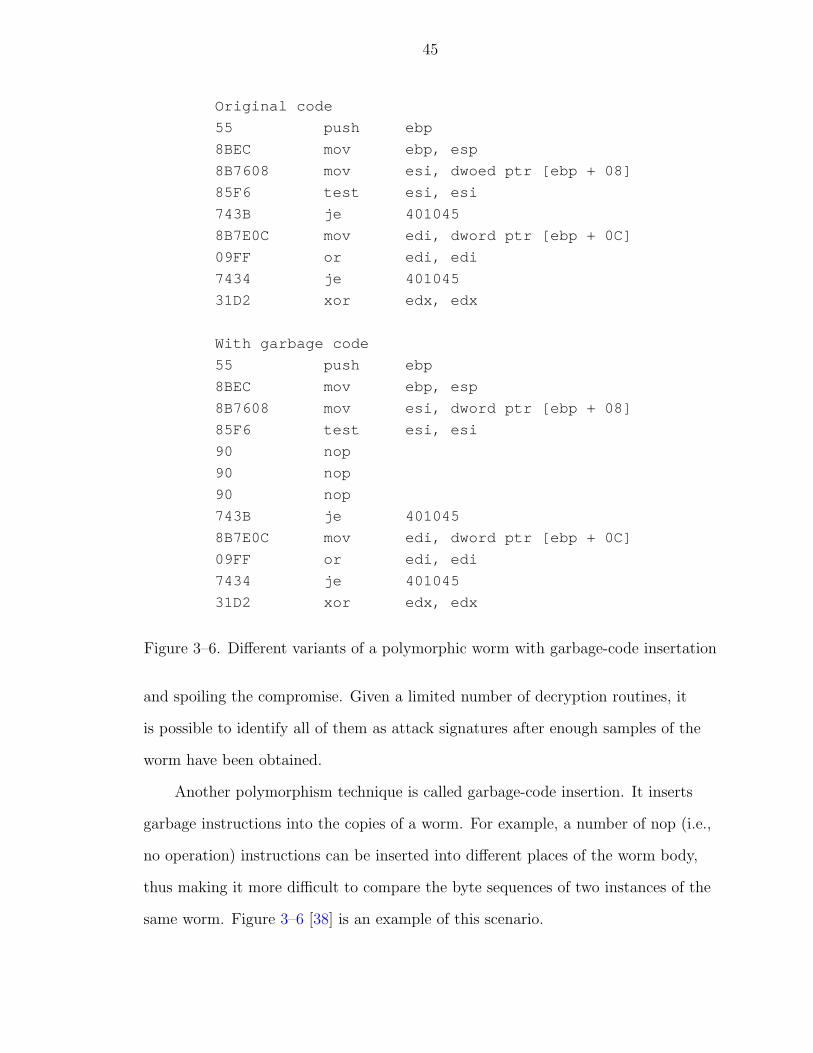
45
Original code
55 push ebp
8BEC mov ebp, esp
8B7608 mov esi, dwoed ptr [ebp + 08]
85F6 test esi, esi
743B je 401045
8B7E0C mov edi, dword ptr [ebp + 0C]
09FF or edi, edi
7434 je 401045
31D2 xor edx, edx
With garbage code
55 push ebp
8BEC mov ebp, esp
8B7608 mov esi, dword ptr [ebp + 08]
85F6 test esi, esi
90 nop
90 nop
90 nop
743B je 401045
8B7E0C mov edi, dword ptr [ebp + 0C]
09FF or edi, edi
7434 je 401045
31D2 xor edx, edx
Figure 3–6. Different variants of a polymorphic worm with garbage-code insertation
and spoiling the compromise. Given a limited number of decryption routines, it
is possible to identify all of them as attack signatures after enough samples of the
worm have been obtained.
Another polymorphism technique is called garbage-code insertion. It inserts
garbage instructions into the copies of a worm. For example, a number of nop (i.e.,
no operation) instructions can be inserted into different places of the worm body,
thus making it more difficult to compare the byte sequences of two instances of the
same worm. Figure 3–6 [38] is an example of this scenario.

46
The level of polymorphism in this type of worms is decided by the ratio of
the length of the garbage instruction region to the total length of the worm. For
those worms with moderate ratio, it is quite conceivable that there will be a good
chance that regions sharing the same byte sequence exist in different instances
of the worms, which in turn can be served as the signature of the worm. With a
increased length, the overlapped regions will be shortened and it is problematic to
identify them.
However, from the statistics point of view, the frequencies of the garbage
instructions in a worm can differ greatly from those in normal traffic. If that
is the case, anomaly-detection systems [4, 14] can be used to detect the worm.
Furthermore, some garbage instructions such as nop can be easily identified and
removed. For better obfuscated garbage, techniques of executable analysis [32] can
be used to identify and remove those instructions that will never be executed.
The instruction-substitution technique replaces one instruction sequence with
a different but equivalent sequence. Unless the substitution is done over the entire
code without compromising the code integrity (which is a great challenge by itself),
it is likely that shorter signatures can be identified from the stationary portion of
the worm. The code-transposition technique changes the order of the instructions
with the help of jumps. The excess jump instructions provide a statistical clue,
and executable-analysis techniques can help to remove the unnecessary jump
instructions. Finally, the register-reassignment technique swaps the usage of the
registers, which causes extensive “minor” changes in the code sequence. These
techniques can be best illustrated in Figure 3–7 [38].
The space of polymorphism techniques is huge and still growing. With the
combinations of different techniques, a cure-all solution is unlikely. The pragmatic
strategy is to enrich the pool of defense tools, with each being effective against
certain attacks. The current defense techniques fall in two main categories,

47
Original code
55 push ebp
8BEC mov ebp, esp
8B7608 mov esi, dwoed ptr [ebp + 08]
85F6 test esi, esi
743B je 401045
8B7E0C mov edi, dword ptr [ebp + 0C]
09FF or edi, edi
7434 je 401045
31D2 xor edx, edx
Obfuscated code
55 push ebp
54 push esp
5D pop ebp
8B7608 mov esi, dword ptr [ebp + 08]
09F6 or esi, esi
743B je 401045
8B7E0C mov edi, dword ptr [ebp + 0C]
85FF test edi, edi
7434 je 401045
28D2 sub edx, edx
558BEC8B760885F6743B8B7E0C09FF743431D2
55545D8B760809F6743B8B7E0C85FF743428D2
Figure 3–7. Different variants of a polymorphic worm with several differentpolymorphic techniques

48
misuse/signature matching and anomaly detection. The former matches against
known patterns in the attack traffic. The latter matches against the statistical
distributions of the normal traffic. We propose a hybrid approach based on a
new type of signatures, consisting of position-aware byte frequency distributions.
Such signatures can tolerate extensive, “local” changes as long as the “global”
characteristics of the signature remain. Good examples are polymorphism caused
by register reassignment and modest instruction substitution. We do not claim
that such signatures are suitable for all attacks. On the other hand, it may work
with executable-analysis techniques to characterize certain statistical patterns that
appear after garbage instructions and excess jumps are removed.
In this paper, we focus on solving the problem of moderate polymorphism.
While we admit that there might exist no unique solution to solve all these
problems, it is quite possible that polymorphism can be at least partially solved
if no extreme case is involved. More importantly, our system is still very useful in
dealing with even the most extreme cases. First of all, our double-honeypot system
is able to automatically capture the different instances of the worm. Although a
unified signature matching all instances of the worm seems unlikely in extreme
cases, it will still help analyzing the behavior of the attack and providing an early
warning of it by capturing the samples of the worm. Second, although it might be
true in some case that human analysis can find out signatures that do not conform
with our model, in most cases it is laborious, empirical, and time-consuming. Our
algorithm, on the other hand, can detect the most subtle signatures based on the
model and is more reliable than human analysis. Finally, our system can cooperate
with other defense systems, e.g., anomaly-based systems, in order to be more
effective.
We use the invariant region of the worm to serve as the signature because we
are dealing with the Internet worms. Other malicious code such as virus can be

49
detected after the machine has been infected by scanning the programs because
virus will rely on the execution of the infected programs. The Internet worms,
however, will need to be identified before the infection has been done as the
goal of the worm is to spread to the Internet as quickly as possible. While some
techniques, e.g. Christodorescu, can successfully identify the polymorphic malicious
code by looking for the semantical equivalence, they are inappropriate in worm
detection as they are unable to be done in real time. In the next section, we use
the iterative algorithms to identify the invariant region from byte sequences of
polymorphic worms.
The basic premise of our model about the signature is that the byte frequency
distributions in the significant region, which in our case is the region that match
the signature approximately, should be greatly different from the rest part of the
worm body and normal, legitimate traffic payloads. The reason is that they carry
different functionalities. For example, in a polymorphic worm, the significant
region is responsible for the true malicious operations while the rest part of the
sequence only serves as a camouflage to elude the defense system. As a result, the
rest part of the sequence will most likely have the same or similar byte frequency
distribution as the legitimate connections. Even if an attacker tries to hide the true
worm body by attaching legitimate payloads, it is always difficult to design a pure
malicious sequence part indistinguishable from the normal connection. Therefore,
the byte frequency distributions related to this part should be under-represented
in the rest of the worm body. If we are able to extract a similar region from each
of the sampled instances of the worm, where the frequency distribution is greatly
different from the rest of the sequence, then this region should be potentially the
significant region and its probabilistic multinomial byte frequency distribution will
be the signature we are looking for.

50
The attackers may not act as what we have expected as above. For example,
they may only insert several nop operations into each instances of the worm
randomly without attaching the camouflage part. Our argument still hold in this
case. Since nop does not appear frequently in normal sessions, the sequence of the
malicious connection will have a high frequency on nop operations. The probability
of nop in each positions will greatly larger than the normal incoming connection
sequence. That is enough to constitute a signature with a width of the same length
as the instances of the worm.
3.3 Position-Aware Distribution Signature (PADS)
3.3.1 Background and Motivation
Most deployed defense systems against Internet worms are signature-based.
They rely on the exact matching of the packet payload with a database of fixed
signatures. Though effective in dealing with the known attacks, they fail to
detect new or variants of the old worms, especially the polymorphic worms whose
instances can be carefully crafted to circumvent the signatures [32]. Moreover,
manually identifying the signatures may take days if not longer.
To address these problems, several anomaly-based systems [4, 14] use the
byte frequency distribution (BFD) to identify the existence of a worm. Their basic
approach is to derive a byte frequency distribution from the normal network
traffic. When a new incoming connection is established, the payload of the packets
is examined. The byte frequency distribution of the connection is computed
and compared with the byte frequency distribution derived from the normal
traffic. A large deviation will be deemed as suspicious. The problem is that an
intelligent attacker could easily cheat the system by attach the worm body to
a lengthy normal, legitimate session. Since the majority of the payload is from
legitimate operations, its byte frequency distribution will not vary much from the

51
normal traffic. As the worm byte sequence is diluted in normal traffic, its statistic
characteristics are smoothed out.
Both signature-based and anomaly-based systems have their pros and cons.
Compared to the anomaly-based systems, signature-based systems have their own
advantages. Since signature-based systems match the signature of the worm with
only the corresponding segment of the whole worm body, it will not help much
to reduce the chance of being detected if normal payloads are attached to the
end of the worm body. However, if only the exact matching is used to compare
the signature with the payloads, a slightly change of the malicious part in the
whole worm body means a mismatch to the signature. In other words, current
signature-based system lacks the flexibility in contrast to the anomaly-based
systems. In addition drawbacks Abe, the signature-based system is not robust
enough to different techniques employed by the intelligent attackers as well. For
example, an attacker might increase the number of garbage instructions inserted to
the worm so that each signature by definition is tailored into only several bytes, as
is shown in figure.X. An automatic signature-extraction system will dramatically
increase the false positives as it is so common that any incoming connections might
contain such a short signature.
Our system inherits the positive aspects of both signature-based and
anomaly-based systems. It is based on a new defense technique that is complementary
to the existing ones. We define a relaxed, inexact form of signatures that have the
flexibility against certain polymorphism. The new signature is called the position-
aware distribution signature (PADS for short). It includes a byte frequency
distribution (instead of a fixed value) for each position in the signature “string”.
The idea is to focus on the generic pattern of the signature while allowing some
local variation.

52
Consider a polymorphic worm with register reassignment (Section 3.2).
Because registers are used extensively in executables, swapping registers is
effective against traditional signatures. However, when a signature is expressed
in position-aware distributions, not only are the static elements in the executable
captured, but the set of likely values for the variable elements are also captured.
Hence, PADS allows a more precise measurement of “matching”. A similar
example is instruction substitution, where the mutually replaceable instructions (or
sequences) can be represented by the position-aware distributions.
To better explain the concept, we give an example here. Suppose a worm
carries a word “worm” in its byte sequence. In order to avoid the detection, the
variants of the worm may change to “w0rm”, “norm”. Counting the number of
byte appearance at each position will give us the following table. Based on this
model, when a new incoming connection is established, it is possible to check the
byte sequence in the connection session and decide the similarity between the
sequence and the previously captured “worm”, “w0rm”, “dorm”, etc.
The goal of our system is to use double honeypots to capture the worm
attack traffic, based on which PADS is derived and used to detect inbound worm
variants. It provides a quick and automatic response that complements the existing
approaches involving human experts. Based on PADS, the defense system will be
able to identify the new variant of a worm at its first occurrence, even if such a
variant has not been captured by the system previously. That means our system
is able to alert the attacks that successfully elude the current existing system,
hence a significant decrease of the false negative. Besides the advantages over the
traditional signature-based system which needs the assistance of the human expert,
our proposed system is especially useful in special cases when an anomaly-based
system may fail.

53
b 0 1 2 ... 9 100x00 0.001 0.001 0.001 ... 0.500 0.1000x01 0.001 0.001 0.001 ... 0.200 0.5000x02 0.005 0.001 0.001 ... 0.001 0.100... ... ... ... ... ... ...
0xfe 0.100 0.001 0.001 ... 0.001 0.0010xff 0.001 0.700 0.700 ... 0.001 0.001
Table 3–1. An example of a PADS signature with width W = 10
3.3.2 Position-Aware Distribution Signature (PADS)
We first describe what is a PADS signature, then explain how to match a byte
sequence against a signature, and finally motivate how to compute such a signature
based on captured worm sequences.
At each byte position p of a PADS signature, the byte-frequency distribution
is a function fp(b), which is the probability for b to appear at position p, where
b ∈ [0..255], the set of possible values for a byte.∑
b∈[0..255] fp(b) = 1. We use
(f1, f2, ...fW ) to characterize the byte-frequency distribution of the worm, where
W is the width of the signature in terms of the number of bytes. Let f0(b)be the
byte frequency distribution of the legitimate traffic. The PADS signature is defined
as Θ = (f0, f1, f2, ...fW ),which consists of a normal signature f0 and an anomalous
signature (f1, f2, ...fW ). Table 3–1 gives an example of a PADS signature with
width W = 10.
When a new connection is established, we need to decide if the payload of the
connection is a variant of the worm or not. It is necessary to define a similarity
scale between a probabilistic byte frequency distribution and a byte sequence.
Consider a set of byte sequences S = S1, S2, ..., Sn, where Si, 1 ≤ i ≤ n,
is the byte sequence of an incoming connection. We want to decide whether Si is
a variant of the worm by matching it against a signature Θ. Let li be the length
of Si. Let Si,1, Si,2, ..., Si,li be the bytes of Si at position 1, 2, ..., li, respectively.
Let seg(Si, ai)be the W -byte segment of Si starting from position ai. The matching
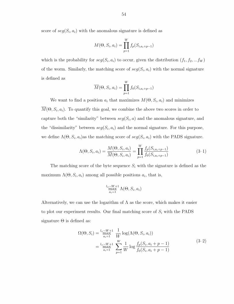
54
score of seg(Si, ai) with the anomalous signature is defined as
M(Θ, Si, ai) =W∏
p=1
fp(Si,ai+p−1)
which is the probability for seg(Si, ai) to occur, given the distribution (f1, f2, ...fW )
of the worm. Similarly, the matching score of seg(Si, ai) with the normal signature
is defined as
M(Θ, Si, ai) =W∏
p=1
f0(Si,ai+p−1)
We want to find a position ai that maximizes M(Θ, Si, ai) and minimizes
M(Θ, Si, ai). To quantify this goal, we combine the above two scores in order to
capture both the “similarity” between seg(Si, a) and the anomalous signature, and
the “dissimilarity” between seg(Si, ai) and the normal signature. For this purpose,
we define Λ(Θ, Si, ai)as the matching score of seg(Si, ai) with the PADS signature.
Λ(Θ, Si, ai) =M(Θ, Si, ai)
M(Θ, Si, ai)=
W∏p=1
fp(Si,ai+p−1)
f0(Si,ai+p−1)(3–1)
The matching score of the byte sequence Si with the signature is defined as the
maximum Λ(Θ, Si, ai) among all possible positions ai, that is,
lx−W+1maxai=1
Λ(Θ, Si, ai)
Alternatively, we can use the logarithm of Λ as the score, which makes it easier
to plot our experiment results. Our final matching score of Si with the PADS
signature Θ is defined as:
Ω(Θ, Si) =lx−W+1maxai=1
1
Wlog(Λ(Θ, Si, ai))
=lx−W+1maxai=1
W∑p=1
1
Wlog
fp(Si, ai + p− 1)
f0(Si, ai + p− 1)
(3–2)

55
The W -byte segment that maximizes Ω(Θ, Si) is called the significant region
of Si, which is denoted as Ri.The matching score of the significant region is the
matching score of the whole byte sequence by definition.
For any incoming byte sequence Si, if Ω(Θ, Si) is greater than a threshold
value, a warning about a (possibly variant) worm attack is issued. Additional
defense actions may be carried out, e.g., rejecting the connection that carries Si.
The threshold is typically set at 0. From the definition of Ω, above zero means that
Si is closer to the anomalous signature (f1, f2, ...fW ); below zero means that Si is
closer to the normal signature f0.
Next we discuss how to calculate Θ based on the previously collected instances
of a worm. Suppose we have successfully obtained a number n of variants of a
worm from the double-honeypot system. Each variant is a byte sequence with
a variable length. It contains one copy of the worm, possibly embedded in the
background of a normal byte sequence. Now let S = S1, S2, ..., Sn be the set of
collected worm variants. Our goal is to find a signature with which the matching
scores of the worm variants are maximized. We attempt to model it as the classical
“missing data problem” in statistics and then apply the expectation-maximization
algorithm (EM) to solve it.
To begin with, we know neither the signature, which is the underlying
unknown parameter, nor the significant regions of the variants, which are the
missing data. Knowing one would allow us to compute the other. We have just
showed how to compute the significant region of a byte sequence if the signature Θ
is know. Next we describe how to compute the signature if the significant regions of
the variants are known.
First we compute the byte frequency distribution for each byte position of the
significant regions. At position p ∈ [1...W ], the maximum likelihood estimation of
the frequency fp(x), x ∈ [0...255], is the number c(p, x) of times that x appears at

56
position p of the significant regions, divided by n.
fp(x) =cp,x
n
One problem is that fp(x) will be zero for those byte values x that never
appear at position p of any significant region. However, considering that our
calculation is based on a limited collection of the variants and fp(x) is only the
maximum likelihood estimation of the frequency, we are not absolutely confident
that the actual frequencies are zero unless we obtain all variants of the worm. For
better flexibility, we apply a “pseudo-count” to the observed byte count cp,x, and
the byte frequency fp(x) is estimated as
fp(x) =cp,x + d
n + 256 · d (3–3)
where d is a small predefined pseudo-count number.
We mentioned in the previous section that anomaly-based systems utilize
the byte frequency distribution to detect the existence of worms. Our method
in this paper is a totally distinct concept. In anomaly-based systems, the
byte frequency distribution of the whole incoming traffic is compared with the
expected distribution of the normal traffic and a great deviation between these
two distributions is considered as malicious. In our method, however, the byte
frequency distribution is used to describe the signature from collected variants of
the same worm only. The purpose is to have a “relaxed” format of the signature
so that the malicious connection can be identified if the payload of the connection
matches to the signature approximately. Variants of the worm need to be obtained
before hand in our systems while anomaly-based systems only need to care about
the patterns of the legitimate traffic.
We have established that the PADS signature and the significant regions
can lead to each other. We do not know either of them, but we know that the

57
significant regions are those segments that can maximize the matching score
with the signature. This “missing data problem” can be solved by an iterative
algorithm, which first makes a guess on the starting positions of the significant
regions, computing the signature, using the signature to compute the new starting
positions of the significant regions, and repeating the process until convergence.
3.4 Algorithms for Signature Detection
In this section, we show how to use the Expectation-Maximization algorithm
and the optimized Gibbs sampling algorithm to compute the PADS signature from
a collection of worm variants captured by our double-honeypot system. We want
to stress that, though comparing the signature with the payload of the incoming
connections is online, the PADS signature itself is computed off-line. There is
no real-time requirement. The purpose of the algorithms is to obtain a PADS
signature that is able to detect the variants of the polymorphic worm even if they
are unknown. If fast response of the worm defense is required, the payloads of
the captured worm variants should be used directly before they go through the
signature center specified. The generated PADS signature can be applied later on
for unobserved variants of the worm.
significant regionbackground
S2
S1
S6
S5
S4
S3
a1
a6
a5
a4
a3
a2
W
Figure 3–8. Signature detection

58
3.4.1 Expectation-Maximization Algorithm
Expectation-Maximization (EM) [35] is an iterative procedure that obtains
the maximum-likelihood parameter estimations. Given a set S of byte sequences,
we lack the starting positions a1, a2, ..., an of the significant regions, which are
the missing data in our problem. The underlying parameter Θ of our data set is
also unknown. The EM algorithm iterates between the expectation step and the
maximization step after the initialization.
The description of EM algorithm is given below.
Initialization. The starting positions a1, a2, ..., an of the significant regions
for worm variants S1, S2, ..., Sn are assigned randomly. They define the initial
guess of the significant regions R1, R2, ..., Rn. The maximum likelihood estimate of
the signature Θ is calculated based on the initial significant regions.
Expectation. The new guess on the locations of the significant regions is
calculated based on the estimated signature Θ. In our algorithm, the new starting
position ai of the significant region is the position that the significant region has
the best match score with the signature Θ. In other words, we seek
ai = arg maxai
Λ(Θ, Si, ai) ∀i ∈ [1..n]
Maximization By formula (3–3), the new maximum likelihood estimate of
the signature Θ is calculated based on the current guess on the locations of the
significant regions.
The algorithms terminates if the average matching score Ω is within (1 + ε) of
the previous iteration, where ε is a small predefined percentage.
Starting with a large signature width W , we run the above algorithm to decide
the signature as well as the significant regions. If the minimum matching score
of all significant regions deviates greatly from the average score, we repeat the

59
algorithm with a smaller W . This process continues until we reach a signature that
matches well with the significant regions of all collected worm variants.
3.4.2 Gibbs Sampling Algorithm
One main drawback of the EM algorithm is that it may get struck in a local
maxima. There is no guarantee that the global maxima can be reached. In order
to solve the problem, many strategies have been proposed. One approach is to
start with multiple random parameter configurations and look for the best among
different results obtained. Another is to pre-process the data with some other
methods and choose “good” initial configuration. In recent years, the simulated
annealing [40] approach attracted great attention. Simply speaking, the approach
allows certain random selection of the parameter (with a small probability moving
towards a worse direction), which provides a chance to jump out of a local maxima.
One example of the simulated annealing is the Gibbs Sampling Algorithm [36],
which we will use to compute the PADS signature below.
The algorithm is initialized by assigning random starting positions for the
significant regions of the worm variants. Then one variant is selected randomly.
This selected variant is temporarily excluded from S. The signature is calculated
based on the remaining variants. After that, the starting position for the significant
region of the selected variant is updated, according to a probability distribution
based on the matching scores at different positions. The algorithm continues with
many iterations until a convergence criterion is met.
The description of the Gibbs sampling algorithm is given below.
Initialization. The starting positions a1, a2, ..., an of the significant regions
for worm variants S1, S2, ..., Sn are assigned randomly.
Predictive Update. One of the n worm variants, Sx, is randomly chosen.
The signature Θ is calculated based on the other variants, S − Sx.

60
The algorithm terminates if the average matching score is within (1 + ε) of the
previous iteration, where ε is a small predefined percentage.
Sampling. Every possible position ax ∈ [1..lx − W + 1] is considered as
a candidate for the next starting position for the significant region of Sx. The
matching score for each candidate position is Λ(Θ, Sx, ax) as defined in (3–1). The
next starting position for the significant region of Sx is randomly selected. The
probability that a position ax is chosen is proportional to Λ(Θ, Sx, ax). That is,
Pr(ax) =Λ(Θ, Sx, ax)∑lx−W+1
ax=1 Λ(Θ, Sx, ax)
Go back to the predictive update step.
Some similarities and difference between EM method and Gibbs sampling
algorithm should be noted here. Both EM method and Gibbs sampler share
the same statistical model built on top of the vocabulary frequencies at each
positions of the predicted common signature region. EM can be thought of as a
deterministic version of Gibbs sampling and Gibbs sampling can also be thought of
as a stochastic analog of the EM algorithm. EM operates on the means of unknown
variables using expected sufficient statistics instead of sampling unknown variables
as does Gibbs sampling. Both EM and Gibbs sampling are used for approximation
with missing data.
3.4.3 Complexities
Since our algorithms are iterative, it makes no sense to discuss the total time
complexity. In stead, we discuss the time and space complexity in each iteration
here. The space complexity in both EM and Gibbs sampling algorithm are fixed
here. During the process, we only need to maintain a relative byte frequency table
of the signature Θ and the start locations of the significant region in each byte
sequence. Therefore, the space complexity is O(256W + n). The time complexity
is quite different. In Gibbs sampling algorithm, each time only one start location

61
is updated. The time complexity in one iteration is O(li −W + 1) since there are
li −W + 1 possibilities. In EM algorithm, we update all start locations at once, the
time complexity is O(∑
i(li −W + 1)) for one iteration. That does not mean Gibbs
sampling is better than EM in time complexity, however. They are generally the
same if updating all start locations is counted as one iteration.
3.4.4 Signature with Multiple Separated Strings
Thus far the PADS signature is assumed to be a continuous string (where
each position in the string is associated not with a byte value but with a byte
frequency distribution). The definition can be easily extended for a signature to
contain k(≥ 1) separated strings, which may have different lengths. The significant
region of a byte sequence also consists of multiple separated segments, each having
a starting position and corresponding to a specific string in the signature. The
matching score Λ(Θ, Si, ai1, ai2, ...) should now be a function of a set of starting
positions, and the significant region is defined by the set of starting positions that
maximizes the matching score. Because it remains that the signature and the
significant regions can be computed from each other, the EM algorithm and the
Gibbs Sampling algorithm can be easily modified to compute a signature with k
strings.
Incorporating models of signature with gaps is necessary and advantageous in
our our system. When polymorphism is used in the worm, an attacker may attach
different variants of the worm to the same legitimate payload. If gaps in signature
are not allowed, the legitimate payload which appears the same in each sampled
byte sequence, instead of worm body that have variations, will be identified by EM
or Gibbs sampling algorithms. With multiple locations and lengths maintained
for one significant region in byte sequence Si, the problem can be solved. By
expanding the total length of the signature with gaps, both the legitimate payload
and the worm body will be covered. In addition, the legitimate payload attached

62
in the signature can be dropped if we compare it with the byte sequences collected
from the legitimate collection session. Therefore, the time and space complexity
can be significantly reduced when we used the simplified signature to check the
incoming traffic.
3.4.5 Complexities
Since our algorithms are iterative, it makes no sense to discuss the total time
complexity. In stead, we discuss the time and space complexity in each iteration
here. The space complexity in both EM and Gibbs sampling algorithm are fixed
here. During the process, we only need to maintain a relative byte frequency table
of the signature Θ and the start locations of the significant region in each byte
sequence. Therefore, the space complexity is O(256W + n). The time complexity
is quite different. In Gibbs sampling algorithm, each time only one start location
is updated. The time complexity in one iteration is O(li −W + 1) since there are
li −W + 1 possibilities. In EM algorithm, we update all start locations at once, the
time complexity is O(∑
i(li −W + 1)) for one iteration. That does not mean Gibbs
sampling is better than EM in time complexity, however. They are generally the
same if updating all start locations is counted as one iteration.
3.5 MPADS with Multiple Signatures
Thus far the PADS signature is defined as a continuous “string” of byte
frequency distributions. It identifies a single significant region in an incoming byte
sequence. This strategy has a couple of limitations. First, a worm may include
a common segment that appears often in normal traffic. This common segment
defeats any attempt by the worm to be polymorphic because the worm is easily
identifiable by the segment. However, it can lure our system to choose the common
segment as the PADS signature and consequently produce false positives on the
normal traffic that happens to carry that segment. Second, a polymorphic worm
may have multiple characteristic segments that all carry useful information. PADS

63
captures the most significant one but discards the rest, which renders it less
powerful against highly sophisticated polymorphic worms.
To address the above limitations, we propose a natural generalization, called
multi-segment position aware distribution signature (MPAD for short), which is
a set of PADS signatures that are combined to identify a worm. It is denoted as
M = (Θ1, ..., Θk), where Θi, 1 ≤ i ≤ k, is a PADS signature. Each PADS signature
may have a different width.
To calculate M, we first use the algorithms in Section 3.4 to compute a PADS
signature, Θ1, and the significant regions for Θ1. We then remove these significant
regions from the worm samples and compute the next PADS signature, Θ2, and the
significant regions for Θ2. We further remove these significant regions and compute
Θ3 ... until there is no more signature that can produce good matching scores for
all worm samples. When an incoming byte sequence is matched against M, it is
classified as a potential worm variant only when its matching scores with all PADS
signatures are above zero. To reduce the matching overhead, the PADS signature
with the most diverse distribution can be used first, which attempts to separate
worm variants (with some false positives) from the background traffic. The rest of
PADS signatures are then applied one after another to progressively filter out the
false positives.
3.6 Mixture of Polymorphic Worms and Clustering Algorithm
Until now we have only discussed how to calculate a PADS/MPAD signature
from a collection of worm variants that belong to the same polymorphic worm.
In reality, multiple different polymorphic worms may rage on the Internet at
the same time, and a double-honeypot system may capture a mixed set of worm
samples that belong to different worms. We have to first partition this mixed set
into clusters, each sharing similar traffic patterns and thus likely to come from
the same worm. This is called cluster partitioning problem. After partitioning, a

64
PADS/MPAD signature is calculated for each cluster. The signatures can then be
used to identify new variants of the worms. We describe two algorithms for the
cluster partitioning problem.
3.6.1 Normalized Cuts
We define a similarity metric between any two variants. A naive definition
is to first compute the byte-frequency distributions of the two variants and
then measure the difference (e.g., KL-divergence) between them. Another naive
definition is to count the length of the longest common substring or the combined
length of the k longest common substrings. A better definition is to compute
a PADS/MPAD signature from the two variants and then take the combined
matching score between the variants and the signature. Our experiments will use
this definition of similarity. Consider two worm variants, Si and Sj. Suppose PADS
is used. Based on (3–2), the similarity between Si and Sj can be expressed as
Ωij = Ω(Θ, Si) + Ω(Θ, Sj)
=li−W+1maxai=1
W−1∑p=0
1
Wlog
fp(Si, ai + p)
f0(Si, ai + p)
+lj−W+1maxaj=1
W−1∑p=0
1
Wlog
fp(Sj, aj + p)
f0(Sj, aj + p)
(3–4)
Where Θ is the PADS signature calculated from Si and Sj and W is the length of
the signature.
The cluster partitioning problem can be formulated in a graph-theoretic
way. We construct a complete graph with n nodes, representing the variants
S = S1, ..., Sn. The edge between Si and Sj is associated with a similarity value
of Ωij as defined in (3–4). Ωii = 0. Given the n × n similarity matrix Π = (Ωij),
i, j ∈ [1..n], we want to find such clusters (e.g., cliques in the graph) that have large
similarity values for intra-cluster edges but small similarity values for inter-cluster
edges. Figure 3–9 illustrates a simple example, where a shorter edge means a larger

65
S3
S1S4
S2
S5
Cluster 1Cluster 2
Figure 3–9. Clusters
similarity value. This is a well-studied problem and a spectral clustering algorithm
called normalized cuts can be used to extract the clusters [41, 42]. For the purpose
of completeness, we briefly describe the algorithm in our context.
The normalized cuts algorithm first decomposes the graph G into two clusters,
A and B, that minimize the following criterion:
cut(A,B)
assoc(A,G)+
cut(A,B)
assoc(B, G)
where cut(A,B) is the sum of the similarity values of all edges that have one end
in A and the other end in B, assoc(A,G) is the sum of the similarity values of all
edges that have one end in A and the other end unrestricted, and assoc(B, G) is
similarly defined.
A vector yis used to define the two clusters. If the ith value of y is 1, then Si
belongs to the first cluster. If it is −1, then Si belongs to the second cluster. In
addition to the similarity matrix Π,we define a degree matrix Das follows
Dii =∑
j
Ωij
for the diagonal elements and zero for all off-diagonal elements.

66
The criterion can then be rewritten as
yT (D − Π)y
yT Dy
Minimizing the above criterion is an integer programming problem if y only take
discrete elements. An approximation is to treat y as a real vector [41] with positive
elements for the first cluster and negative elements for the second cluster. It can be
shown that any y satisfying the following equation for some λ value will minimize
the criterion.
(D − Π)y = λDy
Following certain transformations that we omit here, the generalized eigenvector y
correponding to the second smallest eigenvalue is used [41]. Readers are referred to
[41] for details.
After the algorithm partitions the graph into two clusters, we can recursively
apply the algorithm to further partition each cluster until there is no significant
difference between average intra-cluster similarity and average inter-cluster
similarity.
3.7 Experiments
We perform experiments to demonstrate the effectiveness of the proposed
signatures in identifying polymorphic worms. The malicious payloads of MS
Blaster worm, W32/Sasser worm, Sapphire worm, and a Peer-to-peer UDP
Distributed Denial of Service (PUD) worm are used in the experiments. The MS
Blaster worm exploits a vulnerability in Microsoft’s DCOM RPC interface. Upon
successful execution, MS Blaster worm retrieves a copy of the file msblast.exe from
a previously infected host [43]. The W32/Sasser worm exploits a buffer overflow
vulnerability in the Windows Local Security Authority Service Server (LSASS) on
TCP port 445. The vulnerability allows a remote attacker to execute arbitrary code
with system privileges [44]. For Sapphire (also called Slammer) worm, it caused

67
S2
S1
S5
S4
S3
malicious payload segmentsignificant region
legitimate traffic payload
garbage payloadworm body
a1
a2
a3
a4
a5
Figure 3–10. Variants of a polymorphic worm
considerable harm simply by overloading networks and taking database servers out
of operation. Many individual sites lost connectivity as their access bandwidth was
saturated by local copies of the worm [45]. The PUD worm tries to exploit the SSL
vulnerability on i386 Linux machines [46].
In the experiments, we artificially generate the variants of these worms based
on some polymorphism techniques discussed in Section 3.2. For normal traffic
samples, we use traces taken from the UF CISE network.
Figure 3–10 illustrates the polymorphic worm design with five variants, S1,
S2, ..., and S5. Each variant consists of three different types of regions. The
black regions are segments of the malicious payload in the worm. Substitution
is performed on 10% of the malicious payload. Garbage payloads, which are
represented as the white regions with solid lines, are inserted at different random
locations in the malicious payload. The default ratio of the malicious payload
to the garbage payload is 9:1.1 In addition to garbage payload, each variant is
embedded in the legitimate traffic of a normal session, represented by the white
regions with dotted lines. The length of the normal traffic carried by a worm
1 This ratio is not shown proportionally in Figure 3–10 for better illustration.

68
0 5 10 150
1
2
3
4
5
6
7
8
9
Maximum = 7.5402
avg. no. of recalculations per variant
mat
chin
g sc
ore
(Ω)
Gibbs Run 1Gibbs Run 2Gibbs Run 3EM Run 1EM Run 2EM Run 3
Figure 3–11. Influence of initial configurations
variant is between 2KB to 20KB. In the illustration, the significant regions of these
variants start at a1, a2, ..., and a5, respectively.
3.7.1 Convergence of Signature Generation Algorithms
In the first experiment, 100 variants of MS Blaster worm are generated and
they are used as worm samples for signature generation. The EM algorithm
and the Gibbs Sampling algorithm each run three times with different initial
configurations. Specifically, the initial starting points of significant regions
are randomly selected each time. Figure 3–11 shows the quality of the PADS
signature obtained by EM or Gibbs after a certain number of iterative cycles.
According to Section 3.4, the execution of either algorithm consists of iteration
cycles (Expectation/Maximization steps for EM and Update/Sampling steps for
Gibbs). During each iterative cycle, EM recalculates the significant regions of all
variants, while Gibbs only modifies the significant region of one randomly selected
variant. To make a fair comparison, we let the x axis be the average number of
recalculations performed on the significant region for each variant. The y axis is
the average matching score of the 100 variants with the signature obtained so far.
The matching score Ω is defined in (3–2). From the figure, the best matching score

69
0
50
100
0
50
1003.5
4
4.5
5
5.5
ji
sim
ilarit
y va
lue
(Ωij)
0 20 40 60 80 100−1.5
−1
−0.5
0
0.5
1
1.5
variant id
y
variant 1−−50variant 51−−100
Figure 3–12. Variants clustering using normalized cuts
is around 7.5, which is likely to be the global maxima. EM tends to settle down at
a local maxima, depending on the initial configuration. Gibbs is likely to find the
global maxima but it does not stabilize even when it reaches the global maxima
due to the randomness nature in its selection of starting points of significant
regions.2
3.7.2 Effectiveness of Normalized Cuts Algorithm
The purpose of the second experiment is to evaluate the effectiveness of the
normalized cuts algorithm in solving the cluster partitioning problem. In this
experiment, 50 variants of MS Blaster worm with ids [1..50] and 50 variants of
W32/Sasser worm with ids [51..100] are generated. The normalized cuts algorithm
is used to separate the mixed 100 variants into clusters. The similarity matrix, as
defined in Section 3.6.1 and particularly (3–4), is calculated by using the Gibbs
sampling algorithm. The result is shown in the left-hand plot of Figure 3–12, where
the horizontal axes are variant ids, representing the rows i and the columns j of the
2 The termination condition was not used in this experiment to show thedynamics during the Gibbs iterations.

70
101
102
103
2
3
4
5
6
7
8
9
10
signature width W
mat
chin
g sc
ore
(Ω)
Gibbs−1EM−1Gibbs−2EM−2Gibbs−3EM−3Gibbs−4EM−4
0 1 2 3 4 5 6 7
x 104
0
1
2
3
4
5
6
7
8
9
10
average length of worm variants
mat
chin
g sc
ore
(Ω)
Gibbs−1EM−1Gibbs−2EM−2Gibbs−3EM−3Gibbs−4EM−4
Figure 3–13. Matching score influence of different signature widths and samplevariants lengths
matrix, and the vertical axis is the similarity value between variants i and j. The
surface of the plot can be roughly partitioned into three regions. The first region
(i, j ∈ [1..50]) shows the similarity values amongst the set of MS Blaster worm
variants. The second region (i, j ∈ [51..100]) shows the similarity values amongst
the set of W32/Sasser worm variants. The rest region shows the similarity values
between MS Blaster variants and W32/Sasser variants. By using the normalized
cuts algorithm, the 100 worm variants are separated into two clusters, one for MS
Blaster and one for W32/Sasser. The resulting y vector is shown in the right-hand
plot of Figure 3–12, where each point represents one element in y. The variants
whose values in y are below zero belong to one cluster. The variants whose values
in y are above zero belong to the other cluster.
3.7.3 Impact of Signature Width and Worm Length
In the next set of experiments, we generate 2000 variants of MS Blaster worm,
Sasser worm, Sapphire worm, and PUD worm each. We use 100 samples from
each of the worms for signature generation. The rest 2000 variants are mixed with

71
101
102
103
−5
0
5
10
15
signature width W
mat
chin
g sc
ore
(Ω)
Normal Traffic (Gibbs)Normal Traffic (EM)Worm Traffic (Gibbs)Worm Traffic (EM)Threshold
0 1 2 3 4 5
x 104
−5
0
5
10
15
average length of worm variants
mat
chin
g sc
ore
(Ω)
Normal Traffic (Gibbs)Normal Traffic (EM)Worm Traffic (Gibbs)Worm Traffic (EM)Threshold
Figure 3–14. Influence of different lengths of the sample variants
101
102
103
−5
0
5
10
15
signature width W
mat
chin
g sc
ore
(Ω)
Normal Traffic (Gibbs)Normal Traffic (EM)Worm Traffic (Gibbs)Worm Traffic (EM)Threshold
0 1 2 3 4 5
x 104
−5
0
5
10
15
average length of worm variants
mat
chin
g sc
ore
(Ω)
Normal Traffic (Gibbs)Normal Traffic (EM)Worm Traffic (Gibbs)Worm Traffic (EM)Threshold
Figure 3–15. Influence of different lengths of the sample variants

72
101
102
103
−5
0
5
10
15
signature width W
mat
chin
g sc
ore
(Ω)
Normal Traffic (Gibbs)Normal Traffic (EM)Worm Traffic (Gibbs)Worm Traffic (EM)Threshold
0 1 2 3 4 5
x 104
−5
0
5
10
15
average length of worm variants
mat
chin
g sc
ore
(Ω)
Normal Traffic (Gibbs)Normal Traffic (EM)Worm Traffic (Gibbs)Worm Traffic (EM)Threshold
Figure 3–16. Influence of different lengths of the sample variants
101
102
103
−5
0
5
10
15
signature width W
mat
chin
g sc
ore
(Ω)
Normal Traffic (Gibbs)Normal Traffic (EM)Worm Traffic (Gibbs)Worm Traffic (EM)Threshold
0 1 2 3 4 5
x 104
−5
0
5
10
15
average length of worm variants
mat
chin
g sc
ore
(Ω)
Normal Traffic (Gibbs)Normal Traffic (EM)Worm Traffic (Gibbs)Worm Traffic (EM)Threshold
Figure 3–17. Influence of different lengths of the sample variants

73
normal-traffic byte sequences to test the quality of the signature for each of the
four worms.
Figure 3–13 shows the average matching score with respect to the signature
width and the average length of the worm variants. Because the worm code has a
fixed length, we change the length of a variant by letting it carry a variable amount
of normal traffic. The two figures show the average matching scores of sample
variants after EM and Gibbs sampling algorithms converge to a final signature.
Figure 3–13 also indicates that increasing the signature width will decrease
the average matching score of worm variants. The reason is that a longer signature
means a larger significant region, which increases the chance for the significant
region to include garbage payload, which in turn decreases the matching score.
Figure 3–13 shows that increasing the length of the normal traffic carried by a
worm variant, which has been widely used by some polymorphic worms to elude
the anomaly-based systems, provides no help to avoid detection by our system. The
reason is that our system identifies a significant region and only uses the significant
region for signature generation. The carried normal traffic, no matter how much it
is, will not be used for signature generation.
Figure 3–14– 3–17 show the average matching scores of the testing worm/normal
traffic sequences. The scores for worm traffic are always above zero and the scores
for normal traffic are always below zero. Therefore, with a threshold of 0, worm
variants are distinctively separated from normal traffic. In our experiments, the
generated PADS signature was always able to identify new variants of the worm
without false positive rates. The false positive rate and false negative rate of our
algorithm will be discussed in the next subsection.
3.7.4 False Positives and False Negatives
Figure 3–18 show the false positive rate and false negative rate of our
algorithm for each of the four worms. We only show the influence of signature
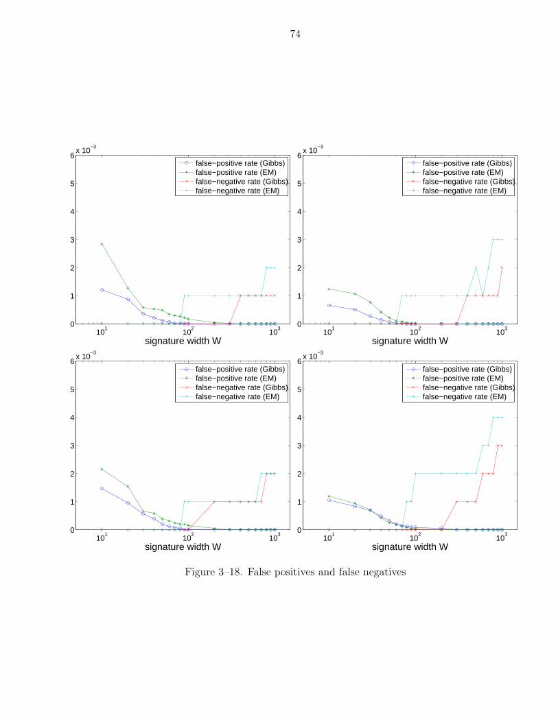
74
101
102
103
0
1
2
3
4
5
6x 10
−3
signature width W
false−positive rate (Gibbs)false−positive rate (EM)false−negative rate (Gibbs)false−negative rate (EM)
101
102
103
0
1
2
3
4
5
6x 10
−3
signature width W
false−positive rate (Gibbs)false−positive rate (EM)false−negative rate (Gibbs)false−negative rate (EM)
101
102
103
0
1
2
3
4
5
6x 10
−3
signature width W
false−positive rate (Gibbs)false−positive rate (EM)false−negative rate (Gibbs)false−negative rate (EM)
101
102
103
0
1
2
3
4
5
6x 10
−3
signature width W
false−positive rate (Gibbs)false−positive rate (EM)false−negative rate (Gibbs)false−negative rate (EM)
Figure 3–18. False positives and false negatives

75
0 20 40 60 80 1000
500
1000
1500
2000
2500
3000
number of sample variants
leng
th o
f sig
natu
relongest common substring method
0 20 40 60 80 100
0
0.2
0.4
0.6
0.8
1
1.2
number of sample variants
fals
e ra
tio
false positive ratiofalse negative ratio
Figure 3–19. The performance of signature-based system using the longest commonsubstrings method.
width because the sample length has little influence on the matching scores. For
all four worm examples, neither false positive nor false negative rate exceed 0.5%.
As we can see from the figure, Gibbs sampling algorithm is always better than
EM algorithm for all four worms. With the increase of signature width, the false
positive rate decreases gradually while false negative rate increases gradually.
3.7.5 Comparing PADS with Existing Methods
For the purpose of comparison, we also perform experiments with some
existing methods. Figure 3–19 shows the experimental results based on the
longest common substring method [30], which first identifies the longest common
substring among the sample worm variants and then uses the substring as a
signature to match against the test variants. Based on the left-hand plot, as the
number of sample variants increase, the length of the longest common substring
decreases. A shorter signature increases the chance for it to appear in normal
traffic. Consequently, the false negative ratio decreases, but the false positive
ratio increases dramatically (the right-hand plot). On the contrary, without the
requirement of exact matching, a PADS signature is able to retain much more
(particularly statistical) characteristics of a polymorphic worm.

76
0 50 100 150 200 2500
0.01
0.02
0.03
0.04
0.05
0.06
0.07
0.08
0.09
0.1
byte value
byte
freq
uenc
y
normal
0 50 100 150 200 2500
0.01
0.02
0.03
0.04
0.05
0.06
0.07
0.08
0.09
0.1
byte valueby
te fr
eque
ncy
worm
Figure 3–20. Byte frequency distributions of normal traffic (left-hand plot) andworm traffic (right-hand plot)
0 50 100 150 200 2500
0.01
0.02
0.03
0.04
0.05
0.06
0.07
0.08
0.09
0.1
byte value
byte
freq
uenc
y
1:1
0 50 100 150 200 2500
0.01
0.02
0.03
0.04
0.05
0.06
0.07
0.08
0.09
0.1
byte value
byte
freq
uenc
y
1:9
Figure 3–21. Byte frequency distributions of worm variants. Left-hand plot:malicious and normal payloads carried by a worm variant have equallength. Right-hand plot: normal payload carried by a worm variant is9 times of malicious payload.

77
Now consider the position-unaware byte frequency distributions that are
used in some current systems. The left-hand plot of Figure 3–20 shows the
position-unaware byte frequency distribution of 100 normal traffic sequences (from
100 normal sessions) and the right-hand plot shows the byte frequency distribution
of MS blaster payload. These two distributions are very different, which seems
provide a way to detect the worm. However, if we create a worm variant by
embedding the worm payload in normal traffic, the combined byte frequency
distribution can be made very similar to that of normal traffic. Figure 3–21
shows the byte frequency distributions of two worm variants whose normal traffic
payloads are 1 and 9 times of malicious payload, respectively. The right-hand plot
is very similar to the left-hand plot of Figure 3–20. Therefore, using byte frequency
distributions alone cannot handle worm variants. The proposed position-aware
distribution signature works better against polymorphic worms.

CHAPTER 4MULTIPLE PADS MODEL AND CLASSIFICATION OF POLYMORPHIC
WORM FAMILIES: AN OPTIMIZATION
4.1 Introduction
As is described in the previous chapters, the iterative methods is a time
consuming process. Because the PADS signature can only be obtained one by one
in the previous method, it will take a long time before every PADS signature has
been extracted. Secondly, because PADS signatures are extracted sequentially, the
quality of the PADS signature will be different. Since iterative methods are used,
different initialization will result in totally different PADS signature set, thus affect
the clustering of the polymorphic worm family. To address these problems, a new
method has to be used to further optimize the previous described approach.
This chapter described a new strategy intended to help identify and detect
the existance of polymorphic Internet worms. The approach tries to improve the
discovery of significant regions for more complicated polymorphism. Compared
with the previous methods, the advantages for the proposed approach are
manyfold. First of all, the significant regions in this approach contain multiple
blocks with no strict sequence. The flexibility allows the detection of more subtle
polymorphism such as code transposition. Secondly, those significant regions that
also appear in normal traffic backgrounds can be effectively removed. Even if the
attacker inserts common normal regions into the polymorphic worms purposely,
the significant region that actually performs the malicious operations can still be
detected. Finally, different types of polymorphic worms are classified simutanously
in order to detect the significant regions more accurately and decrease the false
rate.
78
79
The generation of the PADS block is a “missing data” problem because neither
the malicious regions in each variants of the worm, nor the signature itself is
known. If the malicious regions are known, the PADS block can be calculated by
counting the number of each byte value appearing at different positions. On the
other hand, if the PADS block is known, the malicious region in each variants of
the worm can be obtained by scanning through the whole variants and finding the
regions that best matches the PADS block. The “missing data” problem can be
solved using iterative methods such as Expectation-Maximization (EM) or Gibbs
sampling algorithms which have been mentioned in [47].
The model of the single PADS block in [47] suffers from several limitations.
First of all, a single PADS block can not deal with over-seperated malicious regions
because one PADS block is unlikely to be able to cover all malicious regions.
Secondly, the single PADS block model is unable to exclude the influence of the
background noise. The approach makes an assumption that normal traffic does not
contain the same PADS block, which is not necessary true and can be exploited by
an brilliant attacker. Finally, the model of a single PADS block assumes that each
collected sample of the worm belongs to the same polymorphic worm family. There
is no mechanism to clssify different polymorphic worm families and exclude the
influence of those “outliners”, which will greatly decrease the performance of the
algorithm. In addition to the limitations, the method of extracting PADS blocks
assumes that each sample variant contains exactly one PADS block of the same
type. The sample variants not containing the PADS block will over-contribute
to the characterization of the PADS block and the sample variants containing
repeating PADS blocks will under-contribute.
This paper tries to solve the problem by proposing a multiple PADS blocks
model. In this model, a set of PADS blocks is identified for each polymorphic worm
family, which is identified by a classification method similiar to the extracting

80
of PADS blocks. The signature combines those PADS blocks together and every
PADS blocks within the set are taken into consideration for worm detection. In
order to eliminate the influence of background noise, the common regions within
the normal traffic payload will be first identified and excluded from the sample
worm variant set. Furthermore, the method of extracting PADS blocks in this
paper is able to identify multiple PADS blocks from a mixture of sample variants
that belongs to different polymorphic families, even if some PADS blocks do not
appear in all of the sample variants and some sample variants contains repeating
PADS blocks. To accomplish our goal, we further define a new metric to describe
the quality of the matching between a set of PADS blocks and a byte sequence. It
can be considered as an optimization to the previous described approach.
In the following sections, the details of extracting PADS blocks, the model of
multiple PADS blocks, the signature definition of the multiple PADS model, and
the classification of polymorphic worm families, will be presented, step by step.
4.2 Extraction of Multiple PADS Blocks from the Mixture ofPolymorphic Worms
4.2.1 PADS Blocks and The Dataset from Byte Sequences
In this subsection, we briefly introduce Position-Aware Distribution Signature
(PADS) [47] blocks, which are worm signatures defined in a special format to
identify the malicious regions that appear in all or most of the variants for the
same polymorphic worm.
A PADS block is greatly different from a traditional string signature in that
multinomial byte-frequency distributions replace byte values at each positions of
the PADS block. For a PADS block of width W in terms of the number of bytes,
(f1, ..., fW) is used to characterize the byte-frequency distributions inside the region
of a malicious block, with fk = [fk0, ..., fkb, ...]T for k = 1...W specifying the position

81
k and b = [0...255] for the set of all possible byte values. fkb satisfies:
255∑
b=0
fkb = 1
Table 4–1 is an example of a PADS block with width W .
b f1 f2 ... f9 f10
0x00 0.001 0.001 ... 0.500 0.1000x01 0.001 0.001 ... 0.200 0.5000x02 0.001 0.001 ... 0.001 0.100... ... ... ... ... ...
0xfe 0.001 0.001 ... 0.001 0.0010xff 0.700 0.700 ... 0.001 0.001
Table 4–1. An example of a PADS block with width W = 10
Similiar to the definition of PADS blocks, the multinomial byte-frequency
distribution outside the malicious regions in a byte sequence can be defined as
f0 = [f00, ..., f0b, ...]T with respect to all possible byte value b = [0...255]. We use F
to represent (f1, ..., fW) and f0 respectively in these two cases.
Our purpose is to find the PADS blocks within a mixture of polymorphic
worms. In this paper, each byte sequence Sj is broken up into overlappingly
segments of length W . If aj is used to represent the starting position of a W -byte
segment within a sequence Sj, then aj can be any value between 1 and lj −W + 1,
where lj is the total length of the sequence Sj. By extracting all possible W -byte
segments from the byte sequence set S = S1, S2, ..., a new dataset that contains
all possible W -byte segments is obtained. Suppose N is the total number of
sequences in the dataset, nj is the total number of W -byte segments within a
sequence Sj, and the total number within a sequence set is n. Apparently, we have
n =N∑
j=1
nj =N∑
j=1
(lj −W + 1)
In this paper, the total set of the W -byte segments forms the observed dataset.
To be consistant with the PADS blocks and faciliate the expression, the data of

82
the W -byte segment is represented as byte-frequency distributions as well. Let
G = (g1, ...,gW) be the data of W -byte segment, with gk = [gk1, ..., gkb, ...]T
being the multinomial byte frequency distribution at position k. If the byte value
b appears at the position k of the segment, then gkb = 1 and the rest probabilities
gk1, ..., gk(b−1), gk(b+1), ... are all 0. Table 4–2 is an example of the data for a
W -byte segment.
b g1 g2 ... g9 g10
0x00 0.000 0.000 ... 1.000 0.0000x01 0.000 0.000 ... 1.000 1.0000x02 0.000 0.000 ... 0.000 0.000... ... ... ... ... ...
0xfe 0.000 0.000 ... 0.000 0.0000xff 1.000 1.000 ... 0.000 0.000
Table 4–2. An example of a segment with width W = 10
4.2.2 Expectation-Maximization (EM) Algorithm
We first review the Expectation-Maximization (EM) algorithm before it is
applied in our problem. Let Y = y(1), ...,y(n) be the observed total dataset.
Suppose each data has a mixture density from M groups, with each group decided
by an unknown paramter, then
p(y|θ) =M∑
m=1
πmp(y|θm) (4–1)
where π ≡ π1, ..., πM are mixing probabilities that correspond to the
unknown parameters θ ≡ θ1, ..., θM and satisfy
M∑m=1
πm = 1, πm ≤ 0
It is known that the MLE of the parameter value
θML = arg maxθ
(log p(Y|θ, π)) (4–2)

83
can not be found analytically. The EM algorithm makes use of the concept
of “missing data”. In our model, the missing data is a set of n labels Z =
z(1), ..., z(n) associated with the n observed datas in the dataset, indicating
which group each observed data belongs to. Each label is a binary vector
z(i) = [z(i)0 , ..., z
(i)M ]T . If an observed data y belongs to the m-th group, then
z(i)m = 1 and the data y(i) has the probability p(y(i)|θm). On the other hand, if the
observed data does not belongs to the m-th group, then z(i)m = 0.
Based on the definition of Z, it is straight forward that the prior probability
for z(i)m = 1 is πm,
p(z(i)m = 1|θ, π) = πm (4–3)
The conditional densities of the data y(i) and the missing data z(i) can be written
as
p(y(i)|z(i), θ, π) =M∏
m=1
p(y(i)|θm)z(i)m (4–4)
p(z(i)|θ, π) =M∏
m=1
πmz(i)m (4–5)
The joint density of the observed data y(i) and the missing data z(i) can be
obtained from Eq. 4–4 and 4–5:
p(y(i), z(i)|θ, π) = p(z(i)|θ, π)p(y(i)|z(i), θ, π)
=M∏
m=1
[πmp(y(i)|θm)]z(i)m
(4–6)
Assuming each data is independent, then from Eq. 4–6 we have:
p(Y ,Z|θ, π) =n∏
i=1
M∏m=1
[πmp(y(i)|θm)]z(i)m (4–7)
The complete log-likelihood is
log p(Y ,Z|θ, π) =n∑
i=1
M∑m=1
z(i)m log[πmp(y(i)|θm)] (4–8)
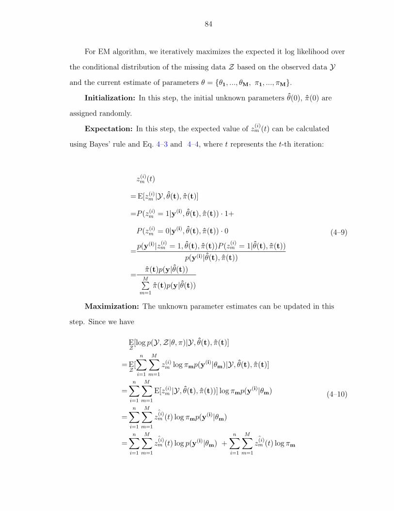
84
For EM algorithm, we iteratively maximizes the expected it log likelihood over
the conditional distribution of the missing data Z based on the observed data Yand the current estimate of parameters θ = θ1, ..., θM, π1, ..., πM.
Initialization: In this step, the initial unknown parameters θ(0), π(0) are
assigned randomly.
Expectation: In this step, the expected value of z(i)m (t) can be calculated
using Bayes’ rule and Eq. 4–3 and 4–4, where t represents the t-th iteration:
z(i)m (t)
= E[z(i)m |Y , θ(t), π(t)]
=P (z(i)m = 1|y(i), θ(t), π(t)) · 1+
P (z(i)m = 0|y(i), θ(t), π(t)) · 0
=p(y(i)|z(i)
m = 1, θ(t), π(t))P (z(i)m = 1|θ(t), π(t))
p(y(i)|θ(t), π(t))
=π(t)p(y|θ(t))
M∑m=1
π(t)p(y|θ(t))
(4–9)
Maximization: The unknown parameter estimates can be updated in this
step. Since we have
EZ[log p(Y ,Z|θ, π)|Y , θ(t), π(t)]
= EZ[
n∑i=1
M∑m=1
z(i)m log πmp(y(i)|θm)|Y , θ(t), π(t)]
=n∑
i=1
M∑m=1
E[z(i)m |Y , θ(t), π(t))] log πmp(y(i)|θm)
=n∑
i=1
M∑m=1
ˆz
(i)m (t) log πmp(y(i)|θm)
=n∑
i=1
M∑m=1
ˆz
(i)m (t) log p(y(i)|θm) +
n∑i=1
M∑m=1
ˆz
(i)m (t) log πm
(4–10)

85
To obtain θm(t + 1), we have
θm(t + 1) = arg maxθm
EZ[log p(Y ,Z|θ, π)|Y , θ(t), π(t)]
= arg maxθm
n∑i=1
ˆz
(i)m (t) log p(y(i)|θm)
(4–11)
To obtain πm(t + 1), we have:
πm(t + 1) = arg maxπm
EZ[log p(Y ,Z|θ, π)|Y , θ(t), π(t)]
= arg maxπm
n∑i=1
M∑m=1
ˆz
(i)m (t) log πm
(4–12)
4.2.3 Extraction of Multiple PADS blocks
We apply the EM algorithm to extract the multiple PADS blocks from the
mixture of polymorphic worms. In our case, the observed data y is the W -width
byte-frequency distributions G = (g1, ...,gW). The unknown parameter θm is the
W -width byte-frequency distributions F = (f1, ..., fW) for 1 ≤ m ≤ M − 1 and
background byte-frequency distribution F = f0 for m = M . Therefore, in the
previous subsection, p(y|θm) can be calculated by:
p(y|θm) =
W∏k=1
255∏b=0
(fkb)gkb ,
if m < M, θm = (f1, ..., fW)m
W∏k=1
255∏b=0
(f0b)gkb ,
if m = M, θm = f0.
(4–13)
Apply the above to Eq. 4–11 and 4–12, we have:
ˆfkb(t + 1) =ˆ
z(i)m (t)gkb/
255∑
b=0
ˆz
(i)m (t)gkb (4–14)
and
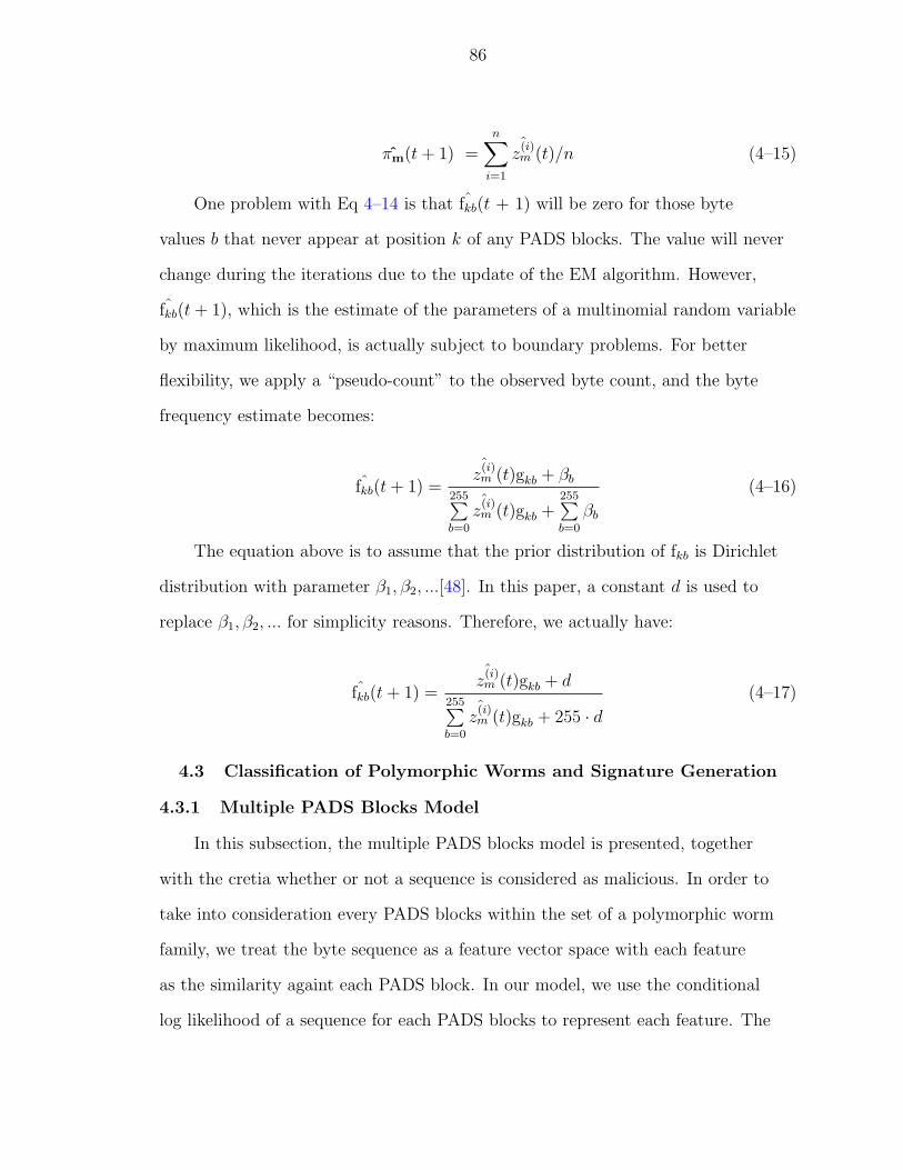
86
πm(t + 1) =n∑
i=1
ˆz
(i)m (t)/n (4–15)
One problem with Eq 4–14 is that ˆfkb(t + 1) will be zero for those byte
values b that never appear at position k of any PADS blocks. The value will never
change during the iterations due to the update of the EM algorithm. However,
ˆfkb(t + 1), which is the estimate of the parameters of a multinomial random variable
by maximum likelihood, is actually subject to boundary problems. For better
flexibility, we apply a “pseudo-count” to the observed byte count, and the byte
frequency estimate becomes:
ˆfkb(t + 1) =
ˆz
(i)m (t)gkb + βb
255∑b=0
ˆz
(i)m (t)gkb +
255∑b=0
βb
(4–16)
The equation above is to assume that the prior distribution of fkb is Dirichlet
distribution with parameter β1, β2, ...[48]. In this paper, a constant d is used to
replace β1, β2, ... for simplicity reasons. Therefore, we actually have:
ˆfkb(t + 1) =
ˆz
(i)m (t)gkb + d
255∑b=0
ˆz
(i)m (t)gkb + 255 · d
(4–17)
4.3 Classification of Polymorphic Worms and Signature Generation
4.3.1 Multiple PADS Blocks Model
In this subsection, the multiple PADS blocks model is presented, together
with the cretia whether or not a sequence is considered as malicious. In order to
take into consideration every PADS blocks within the set of a polymorphic worm
family, we treat the byte sequence as a feature vector space with each feature
as the similarity againt each PADS block. In our model, we use the conditional
log likelihood of a sequence for each PADS blocks to represent each feature. The

87
sequence under the feature space is defined as:
h =
h(1)
h(2)
.
.
h(d)
=
log p(Y |F(1),Π(1))
log p(Y |F(2),Π(2))
.
.
log p(Y |F(d),Π(d))
where F(1),F(2), ...,F(d) are the PADS block signature ( corresponding to θ in the
extraction step ), Π(1),Π(2), ...,Π(d) are the mixturing probabilities ( corresponding
to π in the extraction step ) with respect to F(1),F(2), ...,F(d), and Y is the dataset
y(1),y(2), ...,y(lj−W+1) within a sequence Sj1 .
To fit the multiple PADS model, the signature H for multiple PADS blocks
F(1),F(2), ...,F(d) is defined as a d-dimensional vector as well:
H =
H(1)
H(2)
.
.
H(d)
where H(1), H(2), ..., H(d) specifies the expected value of the conditional log
likelihood for each PADS blocks.
Once the set of PADS blocks and the signature H for the polymorphic worm
family are specified, each sample variant is scored based on how close it is with
respect to the signature H. In our model, Mahalanobis distance is used to measure
the similarity between the feature vector h of any sample variant and the signature
1 Y is different from previously defined Y in that Y is the observed dataset fromall byte sequences.
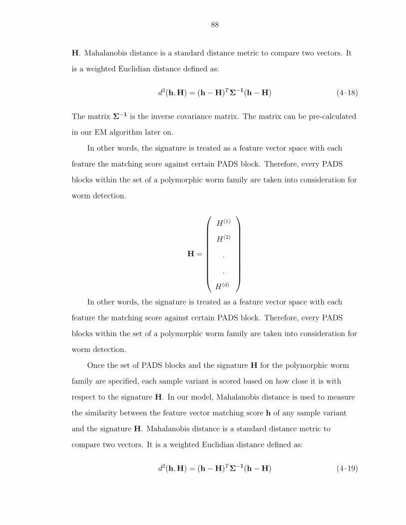
88
H. Mahalanobis distance is a standard distance metric to compare two vectors. It
is a weighted Euclidian distance defined as:
d2(h,H) = (h−H)TΣ−1(h−H) (4–18)
The matrix Σ−1 is the inverse covariance matrix. The matrix can be pre-calculated
in our EM algorithm later on.
In other words, the signature is treated as a feature vector space with each
feature the matching score against certain PADS block. Therefore, every PADS
blocks within the set of a polymorphic worm family are taken into consideration for
worm detection.
H =
H(1)
H(2)
.
.
H(d)
In other words, the signature is treated as a feature vector space with each
feature the matching score against certain PADS block. Therefore, every PADS
blocks within the set of a polymorphic worm family are taken into consideration for
worm detection.
Once the set of PADS blocks and the signature H for the polymorphic worm
family are specified, each sample variant is scored based on how close it is with
respect to the signature H. In our model, Mahalanobis distance is used to measure
the similarity between the feature vector matching score h of any sample variant
and the signature H. Mahalanobis distance is a standard distance metric to
compare two vectors. It is a weighted Euclidian distance defined as:
d2(h,H) = (h−H)TΣ−1(h−H) (4–19)
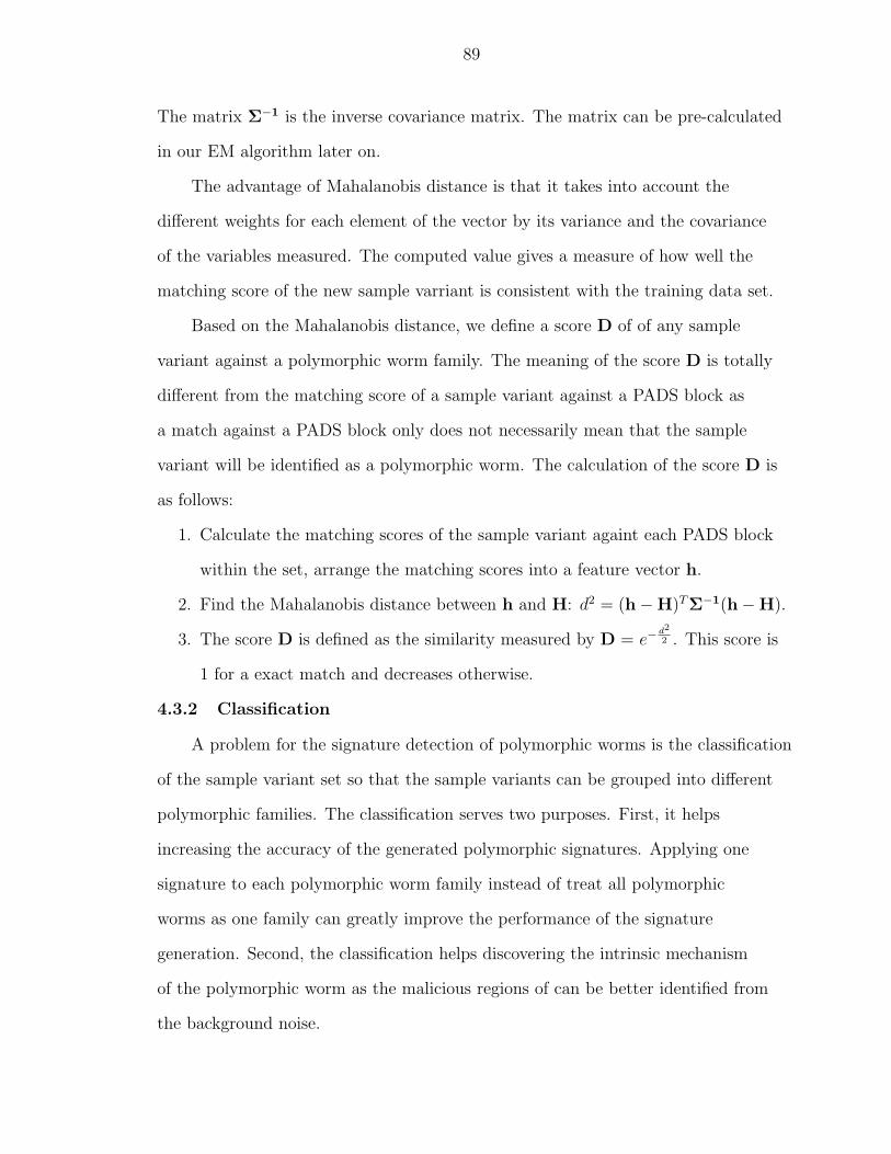
89
The matrix Σ−1 is the inverse covariance matrix. The matrix can be pre-calculated
in our EM algorithm later on.
The advantage of Mahalanobis distance is that it takes into account the
different weights for each element of the vector by its variance and the covariance
of the variables measured. The computed value gives a measure of how well the
matching score of the new sample varriant is consistent with the training data set.
Based on the Mahalanobis distance, we define a score D of of any sample
variant against a polymorphic worm family. The meaning of the score D is totally
different from the matching score of a sample variant against a PADS block as
a match against a PADS block only does not necessarily mean that the sample
variant will be identified as a polymorphic worm. The calculation of the score D is
as follows:
1. Calculate the matching scores of the sample variant againt each PADS block
within the set, arrange the matching scores into a feature vector h.
2. Find the Mahalanobis distance between h and H: d2 = (h−H)TΣ−1(h−H).
3. The score D is defined as the similarity measured by D = e−d2
2 . This score is
1 for a exact match and decreases otherwise.
4.3.2 Classification
A problem for the signature detection of polymorphic worms is the classification
of the sample variant set so that the sample variants can be grouped into different
polymorphic families. The classification serves two purposes. First, it helps
increasing the accuracy of the generated polymorphic signatures. Applying one
signature to each polymorphic worm family instead of treat all polymorphic
worms as one family can greatly improve the performance of the signature
generation. Second, the classification helps discovering the intrinsic mechanism
of the polymorphic worm as the malicious regions of can be better identified from
the background noise.

90
Our method of classification is based on the EM algorithm, which is similiar to
the algorithm we described before. To save the space of the paper, the classification
algorithm is wrapped into a general EM algorithm discussed before. In our
classification algorithm, the observed data y is the d-dimensional h of each byte
sequence. The unknown parameter is the covariance matrix Σ and the signature
H. Different from the model we use in the PADS extraction, we assume h have a
Gaussian mixture density with M families for a d-dimensional random variable h.
Therefore, in the previous section, p(y|θm) is given by:
p(y|θm) =1
(2π)d/2detΣm1/2
e−12(h−Hm)T Σ−1
m (h−Hm)
=1
(2π)d/2detΣm1/2
e−12Dm
(4–20)
Similiar steps can be applied to the general steps of the EM algorithm.
4.4 Conclusion
In this chapter, we further investigate the multiple PADS model and propose
the optimization of our iterative approachs. The iterative methods discussed in
the last subsection suffer from several drawbacks. To address these problems, a
mixture model is used, which assumes that each segment of the dataset may come
from multiple PADS blocks at the same time. It has the clear advantage over
previously proposed approachs in that multiple PADS blocks can be extracted
simultaneously. Furthermore, we define a new metric to define the quality of the
matching between a set of PADS blocks and a byte sequence. To classify different
polymorphic Internet worm families, we also revisit the EM algorithm based on
a Gaussian mixture model for each byte sequence, which is assumed to be in a
feature vector space. The classification or clustering is also done based on an
iterative method (EM). Since both the extraction and the classification only need
one run of iterative methods, the total system can be done within two runs of the
iterative methods. Compared with the previous approach which requires multiple
91
runs of the iterative methods, the newly proposed algorithm further reduces the
time needed for the system.

CHAPTER 5SUMMARY AND CONCLUSION
5.1 Summary
This thesis discusses several novel techniques that detect, slow down, and even
stop the worm propagation over the Internet. Our primary goal is to automate the
anti-worm defense, which is largely a manual process today.
In the first part of the thesis, we proposes a distributed anti-worm architecture
(DAW), which integrates a number of new techniques. DAW detects possible
worm attacks by the edge routers monitoring the local scanning activity and
the management station monitoring the global scanning activity. The scanning
rate is measured based on the rate of failed connection requests, which sets the
worm-infected hosts apart from the normal hosts. DAW ensures sufficient time for
human reaction by the use of a temporal rate-limiting algorithm that constrains the
maximum scanning speed of any infected host and a spatial rate-limit algorithm
that constrains the combined scanning rate of all infected hosts in a network. We
evaluate the performance of DAW both analytically and by simulations, which
demonstrates that DAW is highly effective in damping the propagation of Internet
worms.
In the second part of the thesis, we provide a new defense system to detect the
attacks of malicious Internet worms. The key idea is to capture the samples of the
Internet worm using proposed double-honeypot system before the protected server
has been compromised. Those IP addresses that are unreachable from the outside
are used to attract and trap the attackers. The system is especially useful in large
networks where large number of unreachable IP addresses exist. Our system is
able to defend against polymorphic worms. After collecting a number of variants
92

93
of polymorphic worm, the system uses iterative algorithms to find the PADS
signature of the worm, which is used to detect future worm attacks even if new
variants have not been captured before. In our experiment, a 100% accuracy has
been achieved to detect the variants of MSBlaster worm which means all malicious
traffic can be detected and all legitimate traffic can pass through the system with
no false positives. The system is completely automatic. It requires no involvement
of human experts, which is typically the drawback of the regular signature-based
system. The system also tolerates some modifications of the worm where both
signature- and anomaly-based systems may fail.
In the third part of the thesis, we further investigate the multiple PADS
model and propose the optimization of our iterative approachs. The motivation
for optimization is that the iterative methods discussed in suffer from several
drawbacks. Because the PADS signature can only be obtained one by one and
iterative approachs are time consuming process, it will take a long time before
every PADS signature has been extracted. Because PADS signatures are extracted
sequentially, the quality of the PADS signature will be different. Since iterative
methods are used, different initialization will result in totally different PADS
signature set, thus affect the clustering of the polymorphic worm family. We
propose a new way of extracting multiple PADS blocks at the same time using
iterative methods such as Expectation-Maximization (EM) algorithm. To classify
different polymorphic Internet worm families, we revisit the EM algorithm based
on a Gaussian mixture model for each byte sequence, which is assumed to be in
a feature vector space. The algorithm proposed save the time complexity of the
iterative approachs in that the extraction step can be done simultaneously.
5.2 Conclusion
The contribution of the research that is related to this thesis is threefold.
First of all, a distributed anti-worm architecture (DAW) that automatically slows

94
down or even halts the worm propagation has been developed. DAW is designed
for an Internet service provider to provide the anti-worm service to its customers.
Analytical simulation results have demonstrated the effectiveness of the proposed
techniques. Secondly, a new system called “double-honeypot” system is proposed,
which is able to automatically capture the worm samples over the Internet. Finally,
a new definition of worm signature, which utilizes the statistical properties of the
polymorphic worms, are proposed, together with the new method of automatic
polymorphic worm signature generation. It can effectively identify polymorphic
worms from the normal background traffic. Moreover, it has the capability of
identify future worm attacks even if the worm was not seen before. The paper also
discuss several optimization techniques to reduce the time complexity of iterative
approachs.
REFERENCES
[1] S. Staniford, V. Paxson, and N. Weaver, “How to 0wn the Internet in YourSpare Time,” in Proceedings of the 11th USENIX Security Symposium (Secu-rity ’2002), San Francisco, California, USA, Aug. 2002, pp. 1–20.
[2] D. Moore, C. Shannon, G. M. Voelker, and S. Savage, “Internet Quarantine:Requirements for Containing Self-Propagating Code,” in Proceedings of the22nd Annual Joint Conference of the IEEE Computer and CommunicationsSocieties (INFOCOM ’2003), San Francisco, California, USA, Apr. 2003, pp.1901–1910.
[3] S. Chen and Y. Tang, “Slowing Down Internet Worms ,” in Proceedings of the24th IEEE International Conference on Distributed Computing and Systems(ICDCS ’2004), Tokyo, Japan, Mar. 2004, pp. 312–319.
[4] C. Kruegel and G. Vigna, “Anomaly Detection of Web-based Attacks,” inProceedings of the 10th ACM Conference on Computer and CommunicationSecurity (CCS ’2003). Washington D.C., USA: ACM Press, Oct. 2003, pp.251–261.
[5] D. Moore, V. Paxson, S. Savage, C. Shannon, S. Staniford, and N. Weaver,“Inside the Slammer Worm,” IEEE Magazine of Security and Privacy, pp.33–39, July 2003.
[6] C. Cowan, C. Pu, D. Maier, J. Walpole, P. Bakke, S. Beattie, A. Grier,P. Wagle, Q. Zhang, and H. Hinton, “StackGuard: Automatic AdaptiveDetection and Prevention of Buffer-Overflow Attacks,” in Proceedings of the7th USENIX Security Conference (Security ’1998), San Antonio, Texas, USA,Jan. 1998, pp. 63–78.
[7] M. Eichin and J. Rochlis, “With Microscope and Tweezers: An Analysisof the Internet Virus of November 1988,” in Proceedings of the 1989 IEEESymposium on Security and Privacy, Oakland, California, USA, May 1989, pp.326–344.
[8] J. A. Rochlis and M. W. Eichin, “With Microscope and Tweezers: The Wormfrom MIT’s Perspective,” Commun. ACM, vol. 32, no. 6, pp. 689–698, 1989.
[9] Computer Emergency Response Team. (2001) CERT Advisory CA-2001-23:”Code Red” Worm Exploiting Buffer Overflow In IIS IndexingService DLL. Last accessed: March, 2006. [Online]. Available:http://www.cert.org/advisories/CA-2001-23.html
95

96
[10] ——. (2001) CERT Advisory CA-2001-26: Nimda Worm. Last accessed: March,2006. [Online]. Available: http://www.cert.org/advisories/CA-2001-26.html
[11] ——. (2003) CERT Advisory CA-2001-26: MS-SQL Server Worm. Lastaccessed: March, 2006. [Online]. Available: http://www.cert.org/advisories/CA-2003-04.html
[12] M. M. Williamson, “Throttling Viruses: Restricting Propagation to DefeatMalicious Mobile Code,” in Proceeding of the 18th Annual Computer SecurityApplications Conference (ACSAC ’2002), Las Vegas, Neveda, USA, Oct. 2003,pp. 61–68.
[13] H. Javitz and A. Valdes, “The NIDES Statistical Component Description andJustification,” Computer Science Laboratory, SRI International, Menlo Park,California, USA, Tech. Rep., 1994.
[14] K. Wang and S. J. Stolfo, “Anomalous Payload-based Network IntrusionDetection,” in Proceedings of the 7th International Symposium on RecentAdvances in Intrusion Detection (RAID ’2004), Sophia Antipolis, FrenchRiviera, France, Sept. 2004, pp. 227–246.
[15] K. Ilgun, R. Kemmerer, and P. Porras, “State Transition Analysis: ARule-based Intrusion Detection Approach,” IEEE Trans. Software Eng., vol. 2,pp. 181–199, 1995.
[16] U. Lindqvist and P. Porras, “Detecting Computer and Network Misuse Throughthe Production-Based Expert System Toolset (P-BEST),” in Proceedings of the1999 IEEE Symposium on Security and Privacy, Oakland, California, USA,May 1999, pp. 133–145.
[17] J. O. Kephart and S. R. White, “Directed-Graph Epidemiological Models ofComputer Viruses,” in Proceedings of the 1991 IEEE Symposium on Securityand Privacy, Oakland, California, USA, May 1991, pp. 343–361.
[18] D. Moore, C. Shannon, and K. Claffy, “Code-Red: A Case Study on theSpread and Victims of an Internet Worm,” in Proceedings of the 2nd InternetMeasurement Workshop (IMW ’2002), Marseille, France, Nov. 2002, pp.273–284.
[19] C. C. Zou, W. Gong, and D. Towsley, “Code Red Worm Propagation Modelingand Analysis,” in Proceedings of the 9th ACM Conference on Computer andCommunications Security (CCS ’2002). Washington, DC, USA: ACM Press,Nov. 2002, pp. 138–147.
[20] N. Weaver, I. Hamadeh, G. Kesidis, and V. Paxson, “Preliminary Results UsingScale-down to Explore Worm Dynamics,” in Proceedings of the 2004 ACMWorkshop on Rapid Malcode (WORM ’2004). Washington DC, USA: ACMPress, 2004, pp. 65–72.
97
[21] Z. Chen, L. Gao, and K. Kwiat, “Modeling the Spread of Active Worms,” inProceedings of the 22nd Annual Joint Conference of the IEEE Computer andCommunications Societies (INFOCOM’ 2003), San Francisco, California, USA,Mar. 2003, pp. 1890–1900.
[22] C. C. Zou, L. Gao, W. Gong, and D. Towsley, “Monitoring and Early Warningfor Internet Worms,” in Proceedings of the 10th ACM Conference on Computerand Communication Security (CCS ’2003). Washington D.C., USA: ACMPress, Oct. 2003, pp. 190–199.
[23] J. Twycross and M. M. Williamson, “Implementing and Testing a VirusThrottle,” in Proceedings of the 12th USENIX Security Symposium (Security’2003), Washington D.C., USA, Aug. 2003, pp. 285–294.
[24] S. Schechter, J. Jung, and A. W. Berger, “Fast Detection of Scanning WormInfections,” in Proceedings of the 7th International Symposium on RecentAdvances in Intrusion Detection (RAID ’2004), Sophia Antipolis, FrenchRiviera, France, Sept. 2004, pp. 59–81.
[25] N. Weaver, S. Staniford, and V. Paxson, “Very Fast Containment of ScanningWorms,” in Proceedings of the 13th USENIX Security Symposium (Security’2004), San Diego, California, USA, Aug. 2004, pp. 29–44.
[26] G. Gu, D. Dagon, X. Qin, M. I. Sharif, W. Lee, and G. F. Riley, “WormDetection, Early Warning, and Response Based on Local Victim Information,”in Proceedings of the 20th Annual Computer Security Applications Conference(ACSAC ’2004), Tucson, Arizona, USA, Dec. 2004, pp. 136–145.
[27] S. Staniford, D. Moore, V. Paxson, and N. Weaver, “The Top Speed ofFlash Worms,” in Proceedings of the 2004 ACM Workshop on Rapid Malcode(WORM ’2004). Washington DC, USA: ACM Press, 2004, pp. 33–42.
[28] L. Spitzner, Honeypots: Tracking Hackers. Reading, Massachusetts, USA:Addison-Wesley, 2002.
[29] N. Provos, “A virtual Honeypot Framework,” in Proceedings of the 13th
USENIX Security Symposium (Security ’2004), San Diego, California, USA,Aug. 2004, pp. 1–14.
[30] C. Kreibich and J. Crowcroft, “Honeycomb: Creating Intrusion DetectionSignatures Using Honeypots,” in 2nd Workshop on Hot Topics in Networks(HotNets-II), Cambridge, Massachusetts, USA, Nov. 2003, pp. 51–56.
[31] D. Dagon, X. Qin, G. Gu, W. Lee, J. Grizzard, J. Levin, and H. Owen,“HoneyStat: Local Worm Detection Using Honeypots,” in Proceedings ofthe 7th International Symposium on Recent Advances in Intrusion Detection(RAID ’2004), Sophia Antipolis, French Riviera, France, Sept. 2004, pp. 39–58.

98
[32] M. Christodorescu and S. Jha, “Static Analysis of Executables to DetectMalicious Patterns,” in Proceedings of the 12th USENIX Security Symposium(Security ’2003), Washington D.C., USA, Aug. 2003, pp. 169–186.
[33] O. Kolesnikov and W. Lee, “Advanced Polymorphic Worms: Evading IDS byBlending in with Normal Traffic,” College of Computing, Georgia Institute ofTechnology, Tech. Rep., 2004.
[34] H.-A. Kim and B. Karp, “Autograph: Toward Automated, Distributed WormSignature Detection,” in Proceedings of the 13th USENIX Security Symposium(Security ’2004), San Diego, California, USA, Aug. 2004, pp. 271–286.
[35] C. E. Lawrence and A. A. Reilly, “An Expectation Maximization (EM)Algorithm for the Identification and Characterization of Common Sitesin Unaligned Biopolymer Sequences,” PROTEINS:Structure, Function andGenetics, vol. 7, pp. 41–51, 1990.
[36] C. E. Lawrence, S. F. Altschul, M. S. Boguski, J. S. Liu, A. F. Neuwald, andJ. C. Wootton, “Detecting Subtle Sequence Signals: A Gibbs Sampling Strategyfor Multiple Alignment,” Science, vol. 262, pp. 208–214, Oct. 1993.
[37] H. W. Hethcote, “The Mathematics of Infectious Diseases,” SIAM Review,vol. 42, no. 4, pp. 599–653, 2000.
[38] P. Szor, The Art of Computer Virus Research and Defense. Upper SaddleRiver, New Jersery, USA: Addison Wesley Professional, 2005.
[39] C. Kaufman, R. Perlman, and M. Speciner, Network Security: PrivateCommunication in a Public World. Upper Saddle River, New Jersey, USA:Prentice Hall, Inc., 2002.
[40] S. Geman and D. Geman, “Stochastic Relaxation, Gibbs Distribution, and theBayesian Restoration of Images,” IEEE Trans. Pattern Anal. Machine Intell.,vol. 6, pp. 721–741, 1984.
[41] J. Shi and J. Malik, “Normalized Cuts and Image Segmentation,” IEEE Trans.Pattern Anal. Machine Intell., vol. 22, pp. 888–905, Aug. 2000.
[42] D. A. Forsyth and J. Ponce, Computer Vision A Modern Approach. UpperSaddle River, New Jersey, USA: Prentice Hall, 2003.
[43] Computer Emergency Response Team. (2003) CERT Advisory CA-2003-20:W32/Blaster worm. Last accessed: March, 2006. [Online]. Available:http://www.cert.org/advisories/CA-2003-20.html
[44] United States Computer Emergency Readiness Team. (2004) US-CERT CyberSecurity Bulletin SB04-133. Last accessed: March, 2006. [Online]. Available:http://www.us-cert.gov/cas/body/bulletins/SB04-133.pdf

99
[45] D. Moore, V. Paxson, S. Savage, C. Shannon, S. Staniford, and N. Weaver.(2003) The Spread of the Sapphire/Slammer Worm. Last accessed: March, 2006.[Online]. Available: http://www.caida.org/outreach/papers/2003/sapphire/
[46] C. Hoepers and K. Steding-Jessen. (2003) The Scan of theMonth 25. Last accessed: March, 2006. [Online]. Available:http://www.honeynet.org/scans/scan25/writeup.html
[47] Y. Tang and S. Chen, “Defending Against Internet Worms: A Signature-BasedApproach,” in Proceedings of the 24nd Annual Joint Conference of the IEEEComputer and Communications Societies (INFOCOM ’2005), Miami, Florida,USA, Mar. 2005, pp. 1384–1394.
[48] T. J. Santnerand and D. E. Duffy, The Statistical Analysis of Discrete Data.New York, USA: Springer Verlag, 1989.

BIOGRAPHICAL SKETCH
Yong Tang was born in Kaifeng, China, in 1977. He graduated from Kaifeng
High School and entered Peking University in 1995. After 4 years of study, he
received his Bachelor of Science (B.S.) degree in 1999 with the highest honors.
Since 2002, he has been conducting research with Dr. Shigang Chen in Computer
and Information Science and Engineering Department at the University of Florida.
His research is in the networking and security areas, including Quality-of-Service
(QoS) routing, defense against Distributed Denial-of-Service (DDoS) attacks,
defense against Internet worms, Peer-to-Peer (P2P) networks and wireless
networks.
100