1

Defeasible Reasoning John L. Pollock

Department of Philosophy University of Arizona Tucson, Arizona 85721 pollock@arizona.edu

http://www.u.arizona.edu/~pollock

1. The Inadequacy of Deductive Reasoning

There was a long tradition in philosophy according to which good reasoning had to be deduc-tively valid. However, that tradition began to be questioned in the 1960’s, and is now thoroughly discredited. What caused its downfall was the recognition that many familiar kinds of reasoning are not deductively valid, but clearly confer justification on their conclusions. Here are some simple ex-amples:

Perception Most of our knowledge of the world derives from some form of perception. But clearly, percep-tion is fallible. For instance, I may believe that the wall is grey on the basis of its looking grey to me. But it may actually be white, and it only looks grey because it is dimly illuminated. In this example, my evidence (the wall’s looking grey) makes it reasonable for me to conclude that the wall is grey, but further evidence could force me to retract that conclusion.1 Such a conclusion is said to be justi-fied defeasibly, and the considerations that would make it unjustified are defeaters.

Induction There is one kind of reasoning that few ever supposed to be deductive, but it was often conven-iently ignored when claiming that good reasoning had to be deductive. This is inductive reasoning, where we generalize from a restricted sample to an unrestrictedly general conclusion. For example, having observed a number of mammals and noted that they were all warm-blooded, biologists concluded that all mammals are warm-blooded. Hume’s concern with induction was just that it is not deductive. He should have taken that as an indication that good reasoning need not be deduc-tive, instead of taking that as a reason for worrying about whether it is reasonable to use induction.

Probabilistic reasoning We make essential use of probabilities in reasoning about our place in the world. Most of the generalizations that are justified inductively are probabilistic generalizations rather than exception-less generalizations. For example, I believe that objects usually (with high probability) fall to the ground when released, but I do not believe that this will happen invariably. They might, for exam-ple, be hoisted aloft by a tornado. Still, we want to use these generalizations to predict what is go-

1 One might question whether this is really a case of reasoning. See Pollock and Oved (2006) for a more extensive dis-cussion of this example.

2

ing to happen to us. Because things usually fall to the ground when released, I confidently expect my keys to do so when I drop them. I am surely justified in this belief, although it is only based upon a probabilistic generalization. Because it is based on a probabilistic generalization, it is not a deductive consequence of my reasons for holding it. They make the conclusion reasonable, but I might have to retract it in the face of further information. The form of reasoning involved here is sometimes called the statistical syllogism (Pollock 1990), and has roughly the following form:

From “This is an A and the probability of an A being a B is high”, infer defeasibly, “This is a B”.

Temporal projection Suppose we are standing in a courtyard between two clock towers, and I ask you whether the clocks agree. You look at one, noting that it reads “2:45”, and then you turn to the other and note that it reads “2:45”, so you report that they do. But note that you are making an assumption. You could not look at the two clocks at the same instant, so you are assuming that the time reported by the first clock did not change dramatically in the short interval it took you to turn and look at the second clock. Of course, there is no logical guarantee that this is so. Things change. Our perceptual access to the world is a kind of sampling of bits and pieces at diverse times, and to put the samples together into a coherent picture of the world we must assume that things do not change too rapidly. We have to make a defeasible assumption of stability over times. It might be supposed that we can rely upon induction to discover what properties are stable. We certainly use induction to fine-tune our assumption of stability, but induction cannot provide the origin of that assumption. The difficulty is that to confirm inductively that a property tends to be stable, we must observe that objects possessing it tend to continue to possess it over time, but to do that we must reidentify those objects over time. We do the latter in part in terms of what properties the objects have. For example, if my chair and desk could somehow exchange shapes, locations, colors, and so forth, while I am not watching them, then when I see them next I will reidentify them incorrectly. So the ability to reidentify objects requires that I assume that most of their more salient properties tend to be stable. If I had to confirm that inductively, I would have to be able to reidentify objects without regard to their properties, but that is impossible. Thus a defeasible presumption of stability must be a primitive part of our reasoning about the world.2 A principle to the effect that one can reasonably believe that something remains true if it was true earlier is a principle of temporal projec-tion.

The preceding examples make it clear that we rely heavily on defeasible reasoning for our everyday cognition about the world. The same considerations that mandate our use of defeasible reasoning make it likely that no sophisticated cognizer operating in a somewhat unpredictable environment could get by without defeasible reasoning. The philosophical problem is to understand how defeasible reasoning works.

2 This argument is from chapter six of Pollock (1974).

3

2. A Very Brief History

In philosophy, the study of defeasible reasoning began with Hart’s (1948) introduction of the term “defeasible” in the philosophy of law. Chisholm (1957) was the first epistemologist to use the term, taking it from Hart. He was followed by Toulmin (1958), Chisholm (1966), Pollock (1967, 1970, 1971, 1974), Rescher (1977), and then a number of authors. The philosophical work tended to look only casually at the logical structure of defeasible reasoning, making some simple observa-tions about how it works, and then using it as a tool in analyzing various kinds of philosophically problematic reasoning. Thus, for example, Pollock (1971,1974) proposed to solve the problem of perception by positing a defeasible reason of the form:

“x looks R to me” is a defeasible reason for me to believe “x is R” (for appropriate R).

Without knowing about the philosophical literature on defeasible reasoning, researchers in arti-ficial intelligence rediscovered the concept (under the label “nonmonotonic logic”) in the early 1980’s (Reiter 1980, McCarthy 1980, McDermott and Doyle 1980). They were led to it by their at-tempts to solve the “frame problem”, which I will discuss in detail in section six. Because they were interested in implementing reasoning in AI systems, they gave much more attention to the details of how defeasible reasoning works than philosophers had.3 Unfortunately, their lack of philosophi-cal training led AI researchers to produce accounts that were mathematically sophisticated but epis-temologically naïve. Their theories could not possibly be right as accounts of human cognition, be-cause they could not accommodate the varieties of defeasible reasoning humans actually employ. Although there is still a burgeoning industry in AI studying nonmonotonic logic, this shortcoming tends to remain to this day. I will give a few examples of this below. There are still a number of competing views on the nature and structure of defeasible reasoning. What follows will be a (no doubt biased) account presenting my own views on the matter.

3. Defeasible Reasons and Defeaters

Defeasible reasoning is a form of reasoning. Reasoning proceeds by constructing arguments for conclusions, and the individual inferences making up the arguments are licensed by what we might call reason schemes. In philosophy it is customary to think of arguments as linear sequences of propositions, with each member of the sequence being either a premise or the conclusion of an in-ference (in accordance with some reason scheme) from earlier propositions in the sequence. How-ever, this representation of arguments is an artifact of the way we write them. In many cases the ordering of the elements of the sequence is irrelevant to the structure of the argument. For in-stance, consider an argument that proceeds by giving a subargument for P and an unrelated subar-

3 I believe that I developed the first formal semantics for defeasible reasoning in 1979, but I did not initially publish it because, being ignorant of AI, I did not think anyone would be interested. That semantics was finally published in Pol-lock (1986).

4

gument for (P → Q), and then finishes by inferring Q by modus ponens. We might diagram this ar-

gument as in figure 1. The ordering of the elements of the two subarguments with respect to each other is irrelevant. If we write the argument for Q as a linear sequence of propositions, we must order the elements of the subarguments with respect to each other, thus introducing artificial struc-ture in the representation. For many purposes it is better to represent the argument graphically, as above. Such a graph is an inference graph. The compound arrows linking elements of the inference graph represent the application of reason schemes.

. .

. .

. . P (P → Q)

Q

Figure 1. An inference graph

In deductive reasoning, the reason schemes employed are deductive inference rules. What dis-tinguishes deductive reasoning from reasoning more generally is that the reasoning is not defeasi-ble. More precisely, given a deductive argument for a conclusion, you cannot rationally deny the conclusion without denying one or more of the premises. In contrast, consider an inductive argu-ment. Suppose we observe a number of swans and they are all white. This gives us a reason for thinking that all swans are white. If we subsequently journey to Australia and observe a black swan, we must retract that conclusion. But notice that this does not give us a reason for retracting any of the premises. It is still reasonable to believe that each of the initially observed swans is white. What distinguishes defeasible arguments from deductive arguments is that the addition of informa-tion can mandate the retraction of the conclusion of a defeasible argument without mandating the retraction of any of the earlier conclusions from which the retracted conclusion was inferred. By contrast, you cannot retract the conclusion of a deductive argument without also retracting some of the premises from which it was inferred.

Rebutting defeaters Information that can mandate the retraction of the conclusion of a defeasible argument consti-tutes a defeater for the argument. There are two kinds of defeaters. The simplest are rebutting defeat-ers, which attack an argument by attacking its conclusion. In the inductive example concerning white swans, what defeated the argument was the discovery of a black swan, and the reason that was a defeater is that it entails the negation of the conclusion, i.e., it entails that not all swans are white. More generally, a rebutting defeater could be any reason for denying the conclusion (deduc-tive or defeasible). For instance, I might be informed by Herbert, an ornithologist, that not all swans are white. People do not always speak truly, so the fact that he tells me this does not entail

5

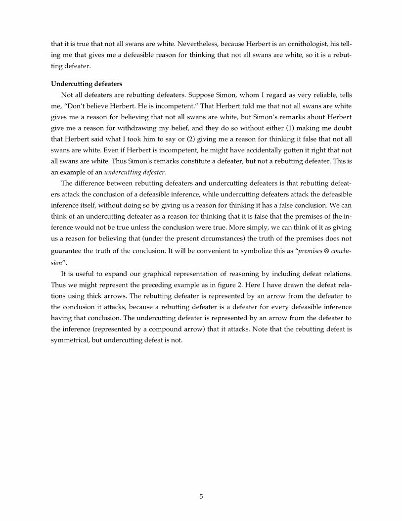
that it is true that not all swans are white. Nevertheless, because Herbert is an ornithologist, his tell-ing me that gives me a defeasible reason for thinking that not all swans are white, so it is a rebut-ting defeater.

Undercutting defeaters Not all defeaters are rebutting defeaters. Suppose Simon, whom I regard as very reliable, tells me, “Don’t believe Herbert. He is incompetent.” That Herbert told me that not all swans are white gives me a reason for believing that not all swans are white, but Simon’s remarks about Herbert give me a reason for withdrawing my belief, and they do so without either (1) making me doubt that Herbert said what I took him to say or (2) giving me a reason for thinking it false that not all swans are white. Even if Herbert is incompetent, he might have accidentally gotten it right that not all swans are white. Thus Simon’s remarks constitute a defeater, but not a rebutting defeater. This is an example of an undercutting defeater. The difference between rebutting defeaters and undercutting defeaters is that rebutting defeat-ers attack the conclusion of a defeasible inference, while undercutting defeaters attack the defeasible inference itself, without doing so by giving us a reason for thinking it has a false conclusion. We can think of an undercutting defeater as a reason for thinking that it is false that the premises of the in-ference would not be true unless the conclusion were true. More simply, we can think of it as giving us a reason for believing that (under the present circumstances) the truth of the premises does not

guarantee the truth of the conclusion. It will be convenient to symbolize this as “premises ⊗ conclu-

sion”. It is useful to expand our graphical representation of reasoning by including defeat relations. Thus we might represent the preceding example as in figure 2. Here I have drawn the defeat rela-tions using thick arrows. The rebutting defeater is represented by an arrow from the defeater to the conclusion it attacks, because a rebutting defeater is a defeater for every defeasible inference having that conclusion. The undercutting defeater is represented by an arrow from the defeater to the inference (represented by a compound arrow) that it attacks. Note that the rebutting defeat is symmetrical, but undercutting defeat is not.

6

swan1 is white swan2 is white … swann is white Ornithologists are reliable sources of information about birds Herbert is Herbert says an ornithologist that not all swans are white Simon says that Herbert Simon is is incompetent reliable All swans [(Herbert is an ornithologist are white & Herbert says that not all swans are white) Not all swans ⊗ are white Not all swans are white]

Figure 2. Inference graph with defeat

We can usefully distinguish between two concepts of a reason. In the preceding example, “Not all swans are white” is inferred from three premises. If we understand the reliability premise as be-ing about probabilities, this can be seen to be an instance of the aforementioned statistical syllo-gism. But notice that it would also be natural to report more simply that our reason for thinking that not all swans are white is that Herbert says they aren’t, ignoring the first two premises. That both ways of talking are natural suggests distinguishing between “full reason schemes” and “en-thymatic reason schemes”. In enthymatic reason schemes, we drop some of the premises that can be regarded as background information, just as we do in an enthymatic argument. For the purpose of understanding how reasoning works, it is best to avoid appeal to enthymatic reason schemes and express our reason schemes in full detail.

4. Semantics for Defeasible Reasoning

We can combine all of a cognizer’s reasoning into a single inference graph and regard that as a representation of those aspects of his cognitive state that pertain to reasoning. The hardest problem in a theory of defeasible reasoning is to give a precise account of how the structure of the cognizer’s inference graph determines what he should believe. Such an account is called a “semantics” for de-feasible reasoning, although it is not a semantics in the same sense as, for example, a semantics for first-order logic. If a cognizer reasoned only deductively, it would be easy to provide an account of what he should believe. In that case, a cognizer should believe all and only the conclusions of his arguments (assuming that the premises are somehow initially justified). However, if an agent rea-sons defeasibly, then the conclusions of some of his arguments may be defeaters for other argu-ments, and so he should not believe the conclusions of all of them. For example, in figure 2, the

7

cognizer first concludes “All swans are white”. Then he constructs an argument for a defeater for the first argument, at which point it would no longer be reasonable to believe its conclusion. But then he constructs a third argument supporting a defeater for the second (defeating) argument, and that should reinstate the first argument. Obviously, the relationships between interacting arguments can be very complex. We want a general account of how it is determined which conclusions should be believed, or to use philosophi-cal parlance, which conclusions are “justified” and which are not. This distinction enforces a further distinction between beliefs and conclusions. When a cognizer constructs an argument, he entertains the conclusion and he entertains the propositions comprising the intervening steps, but he need not believe them. Constructing arguments is one thing. Deciding which conclusions to accept is an-other. What we want is a criterion which, when applied to the inference graph, determines which conclusions are defeated and which are not, i.e., a criterion that determines the defeat statuses of the conclusions. The conclusions that ought to be believed are those that are undefeated. One complication is that a conclusion can be supported by multiple arguments. In that case, it is the arguments themselves to which we must first attach defeat statuses. Then a conclusion is unde-feated iff it is supported by at least one undefeated argument. The only exception to this rule is “ini-tial nodes”, which (from the perspective of the inference graph) are simply “given” as premises. Ini-tial nodes are unsupported by arguments, but are taken to be undefeated. Ultimately, we want to use this machinery to model rational cognition. In that case, all that can be regarded as “given” is perceptual input (construed broadly to include such modes of perception as proprioception, intro-spection, etc.), in which case it may be inaccurate to take the initial nodes to encode propositions. It is probably better to regard them as encoding percepts.4 It is in the computation of defeat statuses that different theories of defeasible reasoning differ. It might seem that this should be simple. The following four principles seem reasonable: (1) A conclusion is undefeated (relative to an inference graph) iff either it is an initial node or it is

supported by at least one undefeated argument in the inference graph. (2) An argument is undefeated iff every inference in the argument is undefeated. (3) If an inference graph contains an undefeated argument supporting a defeater for an inference

used in one of its arguments A, then A is defeated. (4) If an inference graph contains no undefeated arguments supporting defeaters for inferences

used in one of its arguments A, then A is undefeated. It might be supposed that we can apply these four principles recursively to compute the defeat status of any conclusion. For instance, in figure 2, by principle (4), the third argument is undefeated

4 See Pollock (1998) and Pollock and Oved (2006) for a fuller discussion of this.

8

because there are no defeating arguments for any of its inferences and hence no undefeated defeat-ing arguments. Then by principle (3), the second argument is defeated. Then by principle (4), the first argument is undefeated. Finally, by principle (1), the conclusion “All swans are white” is unde-feated.

Collective defeat Unfortunately, there are inference graphs that resist such a simple treatment. For example, con-sider the inference graph of figure 2 without the third argument. The structure of this case can be diagramed more simply as in figure 3, where the dashed arrows indicate defeasible inference. Here we have no arguments lacking defeating arguments, so there is no way for the recursion to get started.

P Q

R ~R

Figure 3. Collective defeat Figure 3 is an example of what is called “collective defeat”, where we have a set of two or more arguments and each argument in the set is defeated by some other argument in the set. What should we believe in such a case? Consider a simple example. Suppose we are in a closed and win-dowless room, and Jones, whom we regard as reliable, enters the room and tells us it is raining out-side. Then we have a reason for believing it is raining. But Jones is followed by Smith, whom we also regard as reliable, and Smith tells us it is not raining. Then we have arguments for both “It is raining” and “It is not raining”, as in figure 3. What should we believe? It seems clear that in the ab-sence of any other information, we should not form a belief about the weather. We should with-hold belief, which is to treat both arguments as defeated. But this means that in cases of collective defeat, an argument is defeated even though its defeating arguments are also defeated. Cases of collective defeat violate principle (4). For example, in figure 3, both R and ~R should be defeated, but neither has an undefeated defeater. Cases of collective defeat are encountered fairly often. An example of some philosophical inter-est is the lottery paradox (Kyburg, 1961). Suppose you hold a ticket in a fair lottery consisting of one million tickets. It occurs to you that the probability of any particular ticket being drawn is one in a million, and so in accordance with the statistical syllogism you can conclude defeasibly that your ticket will not be drawn. Should you throw it away? Presumably not, because that probability is the same for every ticket in the lottery. Thus you get an equally good argument for each ticket that it will not be drawn. However, you are given that the lottery is fair, which means in part that some ticket will be drawn. So you have an inconsistent set of conclusions, viz., for each ticket n you have the conclusion ~Dn that it will not be drawn, but you also have the conclusion that some one of them will be drawn. This generates a case of collective defeat. The lottery paradox can be dia-

9

gramed initially as in figure 4, where R is the description of the lottery. ~D1 contradictory conclusions ~D2 R ~D1 & … & ~D1,000,000 D1 ∨ … ∨ D1,000,000 … ~D1,000,000

Figure 4. The lottery paradox

This can be redrawn as a case of collective defeat by noticing that the set of conclusions ~D1,

~D2,…, ~D1,000,000, D1 ∨ … ∨ D1,000,000 is logically inconsistent. As a result, each subset of the form

~D1, ~D2,…, ~Di-1, ~Di+1,…, ~D1,000,000, D1 ∨ … ∨ D1,000,000

entails the negation of the remaining member, i.e., entails Di. So from each such subset of conclu-sions in the graph we can get an argument for the corresponding Di, and that is a rebutting defeater for the argument to ~Di. More simply, pick one ticket. I have reason to think that it will lose. But I also have a reason to think it will win because I have reason to think that all the others will lose, and I know that one has to win. This yields the inference graph of figure 5. Thus for each conclusion ~Di we can derive the rebutting defeater Di from the other conclusions ~Dj, and hence we have a case of collective defeat. Accordingly, given a theory of defeasible reasoning that can handle infer-ence graphs with collective defeat, the lottery paradox is resolved by observing that we should not conclude of any ticket that it will not be drawn. (Of course, we can still conclude that it is highly un-likely that it will be drawn, but that yields no inconsistency.) ~D1 D1 ~D2 D2 R … D1 ∨ … ∨ D1,000,000 ~D1,000,000 D1,000,000

Figure 5. The lottery paradox as a case of collective defeat

Self-defeat Most theories of defeasible reasoning have some mechanism or other that enables them to get

10

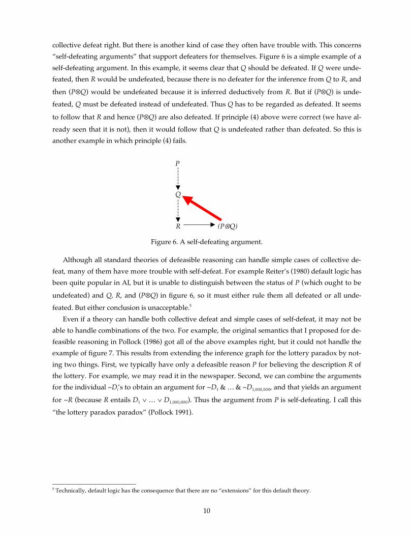
collective defeat right. But there is another kind of case they often have trouble with. This concerns “self-defeating arguments” that support defeaters for themselves. Figure 6 is a simple example of a self-defeating argument. In this example, it seems clear that Q should be defeated. If Q were unde-feated, then R would be undefeated, because there is no defeater for the inference from Q to R, and

then (P⊗Q) would be undefeated because it is inferred deductively from R. But if (P⊗Q) is unde-

feated, Q must be defeated instead of undefeated. Thus Q has to be regarded as defeated. It seems

to follow that R and hence (P⊗Q) are also defeated. If principle (4) above were correct (we have al-

ready seen that it is not), then it would follow that Q is undefeated rather than defeated. So this is another example in which principle (4) fails.

P

Q

R (P⊗Q)

Figure 6. A self-defeating argument.

Although all standard theories of defeasible reasoning can handle simple cases of collective de-feat, many of them have more trouble with self-defeat. For example Reiter’s (1980) default logic has been quite popular in AI, but it is unable to distinguish between the status of P (which ought to be

undefeated) and Q, R, and (P⊗Q) in figure 6, so it must either rule them all defeated or all unde-

feated. But either conclusion is unacceptable.5 Even if a theory can handle both collective defeat and simple cases of self-defeat, it may not be able to handle combinations of the two. For example, the original semantics that I proposed for de-feasible reasoning in Pollock (1986) got all of the above examples right, but it could not handle the example of figure 7. This results from extending the inference graph for the lottery paradox by not-ing two things. First, we typically have only a defeasible reason P for believing the description R of the lottery. For example, we may read it in the newspaper. Second, we can combine the arguments for the individual ~Di’s to obtain an argument for ~D1 & … & ~D1,000,000, and that yields an argument

for ~R (because R entails D1 ∨ … ∨ D1,000,000). Thus the argument from P is self-defeating. I call this

“the lottery paradox paradox” (Pollock 1991).

5 Technically, default logic has the consequence that there are no “extensions” for this default theory.

11

~D1 D1 ~D2 D2 P R … D1 ∨ … ∨ D1,000,000 ~D1,000,000 D1,000,000 ~R ~D1 & … & ~D1,000,000

Figure 7. The lottery paradox paradox

If we distill the self-defeating subargument involving R out of figure 7, we get the inference graph of figure 8. This has the essentially the same structure as figure 4, so if we give it the same treatment we should end up concluding that we are not justified in believing R. That is, we should not believe the description of the lottery we get from the newspaper report. But that is clearly wrong — of course we should believe it. So apparently the other parts of the inference graph change its structure in ways that alter the way the defeat statuses are computed. ~D1 ~D2 P R … ~D1 & … & ~D1,000,000 ~D1,000,000 ~R

Figure 8. The self-defeating argument embedded in the lottery paradox paradox The lottery paradox paradox is a counterexample to the semantics for defeasible reasoning that I proposed in Pollock (1986). Other theories also have trouble with it. For example, simple versions of circumscription (McCarthy 1980) pronounce R defeated when it should not be.6 However, in Pol-lock (1995) I proposed a semantics that yields the intuitively correct answers in all of these exam-ples. My (1995) semantics turns upon principles (1) – (4) above. An inference/defeat loop is a loop con-structed by following a path consisting of inference links and defeat links. When an inference graph contains no inference/defeat loops, there is just one way of assigning defeat statuses that is consis-tent with (1) – (4), and we can compute it recursively. In that case, (1) – (4) seem to give the right answer. But in the presence of inference/defeat loops, there is no way to apply (1) – (4) recursively. 6 There are many forms of circumscription, and by using what are essentially ad hoc prioritization rules it may be possi-ble to get the right answer in figure 7. But because the moves required are ad hoc, I don’t think this shows anything.

12

This reflects the fact that there may be multiple ways of assigning defeat statuses that are consistent with (1) – (4). We cannot apply them recursively to compute defeat statuses because they do not uniquely determine candidate defeat statuses. For example, in figure 3, there are two different ways of assigning defeat statuses to the conclusions making up the inference graph in such a way that principles (1) – (4) are satisfied. This is diagramed in figure 9, where “+” indicates an assignment of “undefeated” and “–” indicates an assignment of “defeated”. The conclusions and arguments that we want to regard as undefeated simpliciter are those that are assigned “+” by all of the ways of assigning defeat statuses consistent with (1) – (4). The lottery paradox works similarly. For each i, there is a way of assigning defeat statuses ac-cording to which ~Di is assigned “–”, but for all j ≠ i, ~Dj is assigned “+”. So again, the conclusions that are intuitively undefeated are those that are always assigned “+”. If we turn to the lottery paradox paradox, the same thing holds. There are the same 1,000,000 assignments of defeat statuses, but now for every one of them ~D1 & … & ~D1,000,000 is assigned “–”, and hence “~R” is assigned “–” and “R” is assigned “+”. Thus we get the desired result that we are justified in believing the description of the lottery, but we are not justified in believing that any par-ticular ticket will not be drawn.

+ P Q +

+ R ~R –

+ P Q +

– R ~R +

Figure 9. Two ways of assigning defeat statuses However, when we turn to the simpler case of self-defeat in figure 6, things become more com-plicated. There is no way to assign defeat statuses consistent with principles (1) – (4). By (1), P must be assigned “+”, which is unproblematic. But there is no way to assign a defeat status to Q. Suppose

we assign “+”. Then we must assign “+” to R and to (P⊗Q). But then we would have to assign “–”

to Q, contrary to our original assignment. If instead we assign “–” to Q, then we must assign “–” to

R and to (P⊗Q). But then we would have to assign “+“ to Q, again contrary to our original assign-

ment. So in this example there can be at most a partial assignment of defeat statuses consistent with (1) – (4). On the other hand, it remains true that the intuitively undefeated conclusions are those that are assigned “+” in all partial status assignments that assign statuses to as many conclusions as

13

possible. Let us define: A partial status assignment is an assignment of defeat statuses (“+” or “–”) to a subset of the con-

clusions and arguments of an inference graph in a manner consistent with principles (1) – (4). A status assignment is a maximal partial status assignment, i.e., a partial status assignment that

cannot be extended to further conclusions or arguments and remain consistent with principles (1) – (4).

My (1995) proposal was then: The defeat status of an argument An argument is undefeated (relative to an inference graph) iff every step of the argument is as-

signed “+” by every status assignment for that inference graph. It would be natural to propose: A conclusion is undefeated (relative to an inference graph) iff it is assigned “+” by every status

assignment for that inference graph. Indeed, this works in all the preceding examples, but that is only because, in those examples, there are no conclusions supported by multiple arguments.7 To see that this does not work in general, consider the case of collective defeat diagramed in figure 10. Once again, there are two status as-

signments. One assigns “+” to R, S, and (S∨T), and “–” to ~R and T. The other assigns “–” to R and

S and “+” to ~R, T, and (S∨T). On both assignments, (S∨T) is assigned “+”. However, there is no ar-

gument supporting (S∨T) all of whose inferences are undefeated relative to both assignments, so

there is no undefeated argument supporting (S∨T). If we regard (S∨T) as undefeated, then we are

denying principle (1), according to which a non-initial node is only undefeated if it is supported by an undefeated argument. However, it seems that principle (1) ought to be true, so instead of the preceding I proposed: The defeat status of a conclusion A conclusion is undefeated iff it is supported by an undefeated argument.

7 This observation is due to Makinson and Schlechta (1991).

14

(R → S) P Q (~R → T)

R ~R

S T

(S∨T)

Figure 10. Collective defeat with multiple arguments This is my (1995) semantics. Its justification is that it seems to give the right answer in all those cases in which it is intuitively clear what the right answer is. This semantics has been implemented in the OSCAR architecture.8 This is an AI system that constitutes an architecture for cognitive agents, and among other things it is a general-purpose defeasible reasoner. Although this semantics is fairly successful, it leaves at least one important question unad-dressed. Reasons have strengths. Not all reasons are equally good, and this should affect the adju-dication of defeat statuses. For example, if I regard Jones as significantly more reliable than Smith, then if Jones tells me it is raining and Smith says it is not, it seems I should believe Jones. In other words, this case of collective defeat is resolved by taking account of the different strengths of the arguments for the conflicting conclusions. An adequate semantics for defeasible reasoning must take account of differences in degree of justification. The preceding semantics only works correctly in cases in which all reasons are equally good. In my (1995) I extended the above semantics to deal with reason strengths, but I am now convinced that the (1995) proposal was not correct. I tried again in my (2002), and that semantics or a minor variation of it may be correct, but I have not yet implemented it in OSCAR. There are currently no other proposals in the AI or philosophical litera-ture for how to perform defeasible reasoning with varying degrees of justification.

5. Defeasible Reasoning v.s. Bayesian Epistemology

There is another approach to non-deductive belief maintenance. This is Bayesian epistemology, which supposes that degrees of justification work like probabilities and hence conflicts can be re-solved within the probability calculus. Bayesians propose that updating one’s beliefs in the face of new information proceeds by conditioning the probabilities of the beliefs on the new information. Conditional probabilities are similar to defeasible reasons in that conditioning on additional infor-mation can lower the probability. That is, prob(P/Q&R) can be lower than prob(P/Q). So it appears that Bayesian epistemology can handle the same phenomena that gave rise to theories of defeasi-

8 The OSCAR architecture is described in my (1995). For up-to-date information on OSCAR, see the OSCAR website at http://oscarhome.soc-sci.arizona.edu/ftp/OSCAR-web-page/OSCAR.html.

15

ble reasoning. There is a huge literature on Bayesian epistemology, but I can only make some brief remarks here.9 One of the most important differences between theories of defeasible reasoning and Baye-sian approaches is that the former accommodate ordinary reasoning—either deductive or defeasi-ble—as a way of deriving new justified beliefs from previously justified beliefs, but the latter do not. For example, theories of defeasible reasoning agree that if the cognizer is initially justified in

believing P and (P → Q), and infers Q from those two premises, then in the absence of a reason for

disbelieving Q, the cognizer becomes justified in believing Q. (Given a reason for ~Q, the argument might instead require the cognizer to give up one of the premises.) By contrast, Bayesian epistemol-ogy makes even deductive reasoning problematic, for reasons I will now explain. The simplest argument against Bayesian epistemology is that it would make it impossible for a conclusion to be justified on the basis of a deductive argument from multiple uncertain premises. This is because, if degrees of justification work like probabilities, then when you combine premises, the degree of justification decreases. Suppose you have 100 independent premises, each with a de-gree of justification of .99. If Bayesian epistemology is correct, then by the probability calculus, the degree of justification of the conjunction will be only .37, so we could never be justified in using these 100 premises conjointly in drawing a conclusion. But this flies in the face of common sense. For example, consider an opinion pollster surveying people about which of two products they pre-fer. She surveys 100 people, collecting from each the verbal expression of an opinion of the form “I prefer x to y”. She summarizes her data by saying, “I surveyed 100 people, and 79 of them reported preferring A to B.” This conclusion follows deductively from her accumulated data. But each piece of data of the form “Person S reported preferring x to y” is something she believes with less than certainty—we are supposing she believes it with a degree of justification of .99. Then if degrees of justification work like probabilities, her degree of justification for thinking that she has surveyed 100 people and 79 of them reported preferring A to B would be at most .37, and hence she would not be justified in drawing that conclusion. Surely this is wrong. Consider another example—counting apples in a barrel. Let us suppose you a very meticulous counter. You examine each apple carefully as you remove it from the barrel, ascertaining that it is indeed an apple, and you then carefully jot down a mark to count the apple so that when you are finished you can read off the result as a number. Let us suppose you are virtually certain you have not lost count (your degree of justification in that is .999), so the only source of uncertainty is in your judgments that the individual objects counted are apples. Suppose you count n apples, judging each to be an apple with a degree of justification j. If degrees of justification work like probabilities, the probability calculus reveals that your degree of justification for believing that there are at least r (r ≤ n) apples in the barrel will be

jr (1 ! r)n! i n!

r !(n ! i)!i= r

i=n

" .

9 See Pollock (2006) for a more extensive discussion.

16

So, for example, if you count 100 apples in the barrel, being justified to degree .95 in believing that each object counted is an apple, then your degree of justification for believing that there are 100 ap-ples in the barrel is only .006. Your degree of justification for believing that there are at least 96 ap-ples in the barrel is only .258. You have to drop all the way down to the judgment that there are at least 95 apples in the barrel before you get a degree of justification greater than .5. If you want a degree of justification of at least .95 for your judgment of the number of apples in the barrel, the best you can do is conclude that there are at least 91. So on this account, you cannot even count ap-ples in a barrel. Similarly, if you have 6 daughters, and your degree of justification for believing of each that she is indeed one of your daughters is .95, then all you can be justified in believing to de-gree .95 is that you have at least 5 daughters. Surely this is ridiculous. Still, there are philosophers (for example, Kyburg 1970) who have been willing to bite the bullet and deny that deductive reasoning from justified premises conveys justification to the conclusion. We can make a distinction between two kinds of deductive inference rules. Let us say that a rule is probabilistically valid iff it follows from the probability calculus that the conclusion is at least as prob-able as the least probable premise. For instance, simplfication and addition are probabilistically valid:

Simplification: (P & Q) w P

Addition: P w (P ∨ Q).

But not all familiar inference rules are probabilistically valid. For example, it is widely recognized that adjunction is not:

Adjunction: P,Q w (P & Q).

In general, prob(P & Q) can have any value between 0 and the minimum of prob(P) and prob(Q). Because of this, Kyburg claims that it is a fallacy to reason using adjunction. He calls this fallacy “conjunctivitis”. For those who are persuaded by these considerations, the view would be that we are only allowed to reason “blindly”, without explicitly computing probabilities (or degrees of justi-fication) as we go along, when the rules of inference we use are probabilistically valid. In all other cases, we must compute the probability of the conclusion to verify that it is still sufficiently probable to be believable. Bayesian epistemology is committed to this view. If degrees of justification satisfy the probability calculus, then without computing probabilities we can only be confident that a de-ductive argument takes us from justified premises to a justified conclusion if all of the inferences are probabilistically valid. Which deductive inference rules are probabilistically valid? It is easily shown that any valid de-ductive inference rule proceeding from a single premise is probabilistically valid. On the other hand, some rules proceeding from multiple premises are not. For example, adjunction is not. Are there others? People are generally amazed to discover that no deductive inference rule that proceeds from multiple premises essentially (that is not still valid if you delete an unnecessary premise) is

17

probabilistically valid. They all go the way of adjunction. For instance, modus ponens and modus tol-lens are not probabilistically valid. Probabilistic validity is the exception rather than the rule. The upshot of this is that if Bayesian epistemology is correct, there will be hardly any deductive reasoning from warranted premises that we can do blindly and still be confident that our conclu-sions are warranted. Blind deductive reasoning can play very little role in epistemic cognition. Epis-temic cognition must instead take the degrees of justification of the premises of an inference and compute a new degree of justification for the conclusion in accordance with the probability calculus. This might not seem so bad until we realize that it is impossible to do. The difficulty is that the probability calculus does not really enable us to compute most probabilities. In general, all the probability calculus does is impose upper and lower bounds on probabilities. For instance, given degrees of justification for P and Q, there is no way we can compute a degree of justification for (P & Q) just on the basis of the probability calculus. It is consistent with the probability calculus for the degree of justification of (P & Q) to be anything from prob(P) + prob(Q) – 1 (or 0 if prob(P) + prob(Q) – 1 < 0) to the minimum of the degrees of justification of P and Q individually. There is in general no way to compute prob(P & Q) just on the basis of logical form. The value of prob(P & Q) is normally a substantive fact about P and Q, and it must be obtained by some method other than mathematical computation in the probability calculus. These observations lead to a general, and I think insurmountable, difficulty for Bayesian episte-mology. Bayesian epistemology claims we must compute degrees of justification as we go along in order to decide whether to accept the conclusions of our reasoning. If conditional degrees of justifi-cation conform to the probability calculus, they will generally be idiosyncratic, depending upon the particular propositions involved. That is, they cannot be computed from anything else. If they can-not be computed, they must be stored innately. This, however, creates a combinatorial nightmare. As Gilbert Harman (1973) observed years ago, given a set of just 300 beliefs, the number of prob-abilities of single beliefs conditional on conjunctions of beliefs in the set is 2300. This is approximately 1090. To appreciate what an immense number this is, a recent estimate of the number of elementary particles in the universe was 1078. So Bayesian epistemology would require the cognizer to store 12 orders of magnitude more primitive probabilities than the number of elementary particles in the universe. This is computationally impossible. Thus Bayesian epistemology would make reasoning impossible. The upshot of this is that if Bayesian epistemology were correct, we could not acquire new justi-fied beliefs by reasoning from previously justified beliefs. However, reasoning is an essential part of epistemic cognition. Without reasoning, all we could know is that our current environment looks and feels various ways to us. It is reasoning that allows us to extend this very impoverished percep-tual knowledge to a coherent picture of the world. So Bayesian epistemology cannot be correct. Cognition requires a different kind of mechanism for updating beliefs in the face of new informa-tion. That is what defeasible reasoning purports to provide.

18

6. Reasoning Defeasibly

In section 4, I discussed how to determine what a cognizer ought to believe given what argu-ments he has constructed. But a theory of rational cognition must also address the question of how the cognizer should go about constructing arguments. In this connection, one can ask how human reasoning works, which is a psychological question, but one can also ask more generally how we can evaluate an arbitrary system of reasoning. For a cognizer that performed only deductive rea-soning, we would presumably want to require that the reasoning be consistent, and we would probably want it to be deductively complete in the sense that the system of reasoning is in principle capable of deriving any deductive consequence of the cognizer’s beliefs. But for a cognizer that rea-sons defeasibly, things are more complicated. There are many systems of automated deductive reasoning in AI. If we focus on reasoners that perform reasoning in the predicate calculus (first-order logic), they are generally sound and com-plete. In other words, they will produce all and only conclusions that follow deductively from whatever premises we give the system. It is natural to suppose that defeasible reasoners should behave similarly. But what is it for them to behave similarly? We need an analogue of deductive validity for defeasible reasoning. Let us say that a conclusion is justified for a cognizer iff it is undefeated relative to the inference graph that encodes all of his reasoning to date. However, for any sophisticated cognizer, reasoning is a non-terminating process. This is true even if the cognizer performs only deductive reasoning in the predicate calculus. However much reasoning the cognizer does, there will always be more that could be done. As a cognizer’s inference graph expands, the cognizer may discover not only argu-ments for new conclusions, but also arguments for defeaters for earlier conclusions. The result is that a previously undefeated conclusion may become defeated just as a result of the cognizer’s per-forming more reasoning, without any addition to the set of initial nodes from which he is reason-ing. This indicates that there are two kinds of defeasibility that we should clearly distinguish. By definition, defeasible reasoning is synchronically defeasible, in the sense that the addition of new in-formation (new initial nodes) can lead previously undefeated conclusions to become defeated. But human reasoning is also diachronically defeasible, in the sense that performing additional reasoning without adding any new information can change the defeat statuses of conclusions. A cognizer’s inference graph consists of all the reasoning it has so far performed. But we can also consider the idealized inference graph consisting of all the reasoning that could be performed given the cognizer’s current initial nodes. Let us say that a proposition (it may not yet be a conclu-sion) is warranted for the cognizer iff it is undefeated relative to this idealized inference graph. So warrant is justification in the limit. The set of warranted propositions is, in effect, the target at which defeasible reasoning aims. Analogous to requiring a deductive reasoner to be sound and complete, we might require a de-feasible reasoner to produce all and only warranted conclusions. This is precisely the requirement that has generally been imposed on automated defeasible reasoners in AI. However, for reasons that have been well known since 1980, no defeasible reasoner capable of performing sophisticated

19

reasoning (e.g., reasoning that includes deductive reasoning in the predicate calculus) can satisfy this requirement. It is mathematically impossible. I will explain. For the predicate calculus, it is possible to build an automated reasoner that draws all and only valid conclusions because the set of valid conclusions is recursively enumerable. A recursively enu-merable set is one for which there is a mechanical procedure (an algorithm) for systematically gen-erating all the members of the set in such a way that no non-members are ever generated by the procedure. Proof procedures for the predicate calculus are such procedures, and hence the com-pleteness theorem for the predicate calculus tells us that the set of valid formulas is recursively enumerable. Automated theorem provers for the predicate calculus take advantage of this by im-plementing such a mechanical procedure. But when we turn to defeasible reasoning, nothing similar is possible. This is because, as Reiter (1980) and Israel (1980) observed, the set of warranted conclusions will not generally be recursively enumerable. Suppose, for instance, that we have a defeasible reasoner that uses a first-order lan-guage (i.e., the language contains the quantifiers and connectives of the predicate calculus). Suppose it makes a defeasible inference to a conclusion P. A necessary condition for P to be warranted is that ~P not be a theorem of the predicate calculus, for if ~P were a theorem, that would constitute de-feat. If the system had to wait until it has determined that P is not defeated before adding it to its set of beliefs, it might have to wait forever. The difficulty is that, by Church’s theorem, the set of non-theorems of the predicate calculus is not recursively enumerable. Thus there is no mechanical pro-cedure for verifying that ~P is not a theorem. If it isn’t then no matter what algorithms the reasoner employs, it may never discover that fact, and so it will never be in a position to affirm P. This is a mathematical constraint on any system of defeasible reasoning. If it waits to affirm a conclusion until it has determined conclusively that the conclusion is undefeated, there will be many warranted conclusions that it will never be in a position to affirm, so it will not produce all war-ranted conclusions. On the other hand, if it does not wait, then it will sometimes get things wrong and affirm conclusions that are justified given the current stage of its reasoning but not warranted. All automated defeasible reasoners except OSCAR are crippled by this problem. Because they assume that a defeasible reasoner should work like a deductive reasoner, and produce all and only warranted conclusions, they restrict themselves to reasoning in very impoverished languages in which both the set of deductively valid formulas and the set of deductively invalid formulas are re-cursively enumerable. Technically, these are languages that are decidable. Unfortunately, only very weak and inexpressive languages are decidable. Thus with the exception of OSCAR, all automated defeasible reasoners tend to work only in the propositional calculus or some even less expressive subset of it. Obviously, humans are not so constrained. How do humans avoid this difficulty? They do so by reasoning defeasibly. In other words, they draw conclusions with the expectation that they will occa-sionally have to retract them later. They don’t wait for an absolute guarantee of warrant. After all, we draw conclusions in order to help us decide how to act. But we cannot wait for the end of a non-terminating process before deciding how to act. Decisions have to be based on what we currently believe, on our justified beliefs, not on the ideal set of warranted propositions. Any sophisticated

20

defeasible reasoner must work similarly. OSCAR does the same thing humans do here. That is, OSCAR draws conclusions on the basis of its current reasoning, and when it has to decide how to act it bases its decision on its current beliefs, but as both reasoning and the input of new informa-tion proceed, it may have to withdraw some of its beliefs. This means that, occasionally, it will have acted in ways it would not have acted had it had time to do more reasoning. But that does not show that there is something wrong with OSCAR, or that OSCAR is behaving irrationally. It is just a fact of life that cognizers, human or otherwise, will make mistakes as a result of not knowing certain things that would have helped. Some of these mistakes will result from the cognizer not having ac-quired relevant information perceptually, but other mistakes will result from the cognizer not hav-ing time to do enough reasoning. This is just the way cognition works, and it is unrealistic to sup-pose we could completely avoid either source of mistakes through clever engineering.

7. Illustration: The Frame Problem

In philosophy, most work on defeasible reasoning has been aimed at using it as a tool for the analysis of philosophically interesting kinds of reasoning — mainly in epistemology but also in the philosophy of law. In AI, on the other hand, the investigation of defeasible reasoning was moti-vated by the desire to build implemented systems that could solve certain kinds of problems. One problem of interest to both philosophers and AI researchers is the frame problem, so I will use it as an illustration of the importance of understanding defeasible reasoning in order to understand how rational cognition works.

7.1 What is the Frame Problem? There is a great deal of confusion about just what the frame problem is, so I will begin with a brief history. The frame problem arose initially in AI planning theory. Planning theory is concerned with the construction of automated systems that will produce plans for the achievement of specified goals. In order to construct a plan, an agent must be able to predict the outcomes of the various ac-tions that a plan might prescribe. For this purpose, let us suppose the agent has all the general background knowledge it might need. Consider a very simple planning problem. The agent is standing in the middle of a room, and the light is off. The light switch is by the door. The agent wants the light to be on. The obvious plan for achieving this goal is to walk to the vicinity of the light switch and activate the switch. We human beings can see immediately that, barring unforeseen difficulties, this is a good plan for achieving the goal. If an artificial agent is to be able to see this as well, it must be able to infer that the execution of this plan will, barring unforeseen difficulties, achieve the goal. The reasoning required seems easy. First, the switch is observed to be in position S. Our background knowledge allows us to infer that if we walk towards position S, we will shortly be in that vicinity. Second, our background knowledge allows us to infer that when we are in the vicinity of the switch, we can activate it. Third, it informs us that when we activate the switch, the light will come on. It may seem that this information is all that is required to conclude that if the plan is executed then the light will come on. But in fact, one more premise is required. We know

21

that the switch is initially in position S. However, for the plan to work, we must know that the switch will still be in position S when we get there. In other words, we have to know that walking to position S does not change the position of the switch. This of course is something that we do know, but what this example illustrates is that reasoning about what will change if an action is per-formed or some other event occurs generally presupposes knowing that various things will not change. Early attempts in AI to model reasoning about change tried to do so deductively by formulating axioms describing the environment in which the planner was operating and then using those axi-oms to deduce the outcomes of executing proposed plans. The preceding example illustrates that among the axioms describing the environment there must be both causal axioms about the effects of various actions or events under specified circumstances, and a number of axioms about what does not change when actions are performed or events occur under specified circumstances. The latter axioms were called frame axioms.10 In our simple example, we can just add a frame axiom to the effect that the switch will still be in position S if the agent walks to that position, and then the requisite reasoning can be performed. However, in pursuing this approach, it soon became appar-ent that more complicated situations required vastly more (and more complicated) frame axioms. A favorite example of early AI researchers was the Blocks World, in which children’s building blocks are scattered about and piled on top of each other in various configurations, and the planning prob-lem is to move them around and pile them up in a way that results in the blocks being arranged in some desired order. If we make the world sufficiently simple, then we can indeed axiomatize it and reason about it deductively. But if we imagine a world whose possibilities include all the things that can happen to blocks in the real world, this approach becomes totally impractical. For instance, moving a block does not normally change its color. But it might if, for example, an open can of paint is balanced precariously atop the block. If we try to apply the axiomatic approach to real-world situations, we encounter three problems. First, in most cases we will be unable to even for-mulate a suitable set of axioms that does justice to the true complexity of the situation. But second, even if we could, we would find it necessary to construct an immense number of extraordinarily complex frame axioms. And third, if we then fed these axioms to an automated reasoner and set it the task of deducing the outcomes of a plan, the reasoner would be forced to expend most of its re-sources reasoning about what does not change rather than what does change, and it would quickly bog down and be unable to draw the desired conclusions about the effects of executing the plan.11 The upshot of this is that in realistically complicated situations, axiomatizing the situation and reasoning about it deductively is made unmanageable by the proliferation and complexity of frame axioms. What became known as the frame problem is the problem of reorganizing reasoning about change so that reasoning about non-changes can be done efficiently.12 Unfortunately, some philosophers have confused the frame problem with other rather distantly related problems, and this has confused its discussion in philosophy and cognitive science. For ex- 10 McCarthy and Hayes (1969). 11 On this last point, the reader who lacks experience with automated reasoners will have to take my word, but this is a point about which no AI practitioner would disagree. 12 McCarthy and Hayes (1969).

22

ample, Fodor (2001) takes the frame problem to be the general problem of how to reason effi-ciently against the background of a large database of information. That is indeed a problem, but a solution to it would not tell us how to reason about change. The frame problem arose in AI, and it has often gone unappreciated that it is equally a problem for human epistemology. Humans can perform the requisite reasoning, so they instantiate a solu-tion to the frame problem. However, it is not obvious how they do it, any more than it is obvious how they perform inductive reasoning or probabilistic reasoning or any other epistemologically problematic species of reasoning. Describing such reasoning is a task for epistemology. Further-more, it seems quite likely that the best way to solve the frame problem for artificial rational agents is to figure out how it is solved in human reasoning and then implement that solution in artificial agents. Thus the epistemological problem and the AI engineering problem become essentially the same problem. The frame problem arose in the context of an attempt to reason about persistence and change deductively. That may seem naive in contemporary epistemology, where it is now generally agreed that most of our reasoning is defeasible, but it should be borne in mind that at the time this work was taking place (the late 1960’s), philosophy itself was just beginning to appreciate the neces-sity for nondeductive reasoning, and at that time the predominant view was still that good argu-ments must be deductively valid. Thirty five years later, nobody believes that. Some kind of defea-sible reasoning is recognized as the norm, with deductive reasoning being the exception. To what extent does the frame problem depend upon its deductivist origins? This same question occurred to AI researchers. Several authors proposed eliminating frame axi-oms altogether by reasoning about change defeasibly and adopting some sort of defeasible infer-ence scheme to the effect that it is reasonable to believe that something doesn’t change unless you are forced to conclude otherwise.13 This is what I called “temporal projection” in section one. Im-plementing temporal projection was the original motivation in AI for research on defeasible rea-soning and nonmonotonic logic.14 Let us consider how temporal projection can be formulated using the system of defeasible reasoning discussed above. Then I will return to its use in the frame prob-lem.

7.2 Temporal Projection In section one I argued that in order for cognition to work a cognitive agent must have a built-in presumption that the objects tend to have their properties stably. In other words, that an object has a property at one time gives us a defeasible reason for expecting that it will still have that property at a later time. The built-in epistemic arsenal of a rational agent must include reason-schemes of the following sort for at least some choices of P: (1) If t0 < t1, believing P-at-t0 is a defeasible reason for the agent to believe P-at-t1.

13 Sandewall (1972), McDermott (1982), McCarthy (1986). 14 For example, see the collection of papers in Ginsberg (1987).

23

Some such principle as (1) is of crucial importance in enabling an agent to combine the results of dif-ferent perceptual samplings of the world into unified conclusions about the world. Without this, the agent would be stuck in separate time-slices of the world with no way to bridge the boundaries epistemically. Principle (1) amounts to a presumption that P’s being true is a stable property of a time. A stable property is one for which the probability is high that if it is possessed at one time, it will continue to

be possessed at a later time. Let ρ be the probability that P will hold at time t+1 given that it holds at

time t. I will not prove this here, but assuming independence, it follows that the probability that P

will hold at time (t+Δt) given that it holds at time t is ½(2ρ – 1)Δt + ½. In other words, the strength of

the presumption that a stable property will continue to hold over time decays towards .5 as the time interval increases. In a system of defeasible reasoning that accommodates varying degrees of justification, this should be built into the principles of temporal projection by making the strength

of the reason a monotonic decreasing function of Δt. However I will not discuss this further here.

7.3 Temporal Projectibiity Principle (1) is not yet an adequate formulation of temporal projection. It takes little reflection to see that there must be some restrictions on what propositions P it applies to. For example, knowing that it is now 3 PM does not give me a defeasible reason for thinking it will still be 3 PM in an hour. Surprisingly, it turns out that certain kinds of logical composition also create problems in connec-tion with principle (1). For example, we must in general be barred from applying temporal projec-tion to disjunctions. This is illustrated by figure 11. Let P and Q be unrelated propositions. In the in-ference-graph of figure 11, the thin solid arrows symbolize deductive inferences. In this inference-

graph, the conclusion Q-at-t2 is undefeated. But this is unreasonable. Q-at-t2 is inferred from (P∨Q)-

at-t2. (P∨Q) is expected to be true at t2 only because it was true at t1, and it was only true at t1 be-

cause P was true at t1. This makes it reasonable to believe (P∨Q)-at-t2 only insofar as it is reasonable

to believe P-at-t2, but the latter is defeated.

24

P-at-t1

(P∨Q)-at-t1

P-at-t2

(P∨Q)-at-t2 ~P-at-t2

Q-at-t2

Figure 11. Temporal projection with disjunctions Just to have a label for the propositions to which temporal projection can be properly applied, let us say they are temporally projectible. The principle of temporal projection can then be formulated as follows: Temporal-projection

If P is temporally-projectible then believing P-at-t is a defeasible reason for the agent to believe

P-at-(t+ Δt), the strength of the reason being a monotonic decreasing function of Δt.

However, we still need an account of temporal projectibility. That is hard to come by. It seems that the ascriptions of “simple” properties to objects will generally be projectible. For instance, “x is red” would seem to be temporally projectible. When we turn to logical compounds, it is easily proven that conjunctions of temporally projectible propositions are temporally projectible (Pollock 1998). But as we have seen, disjunctions of temporally projectible propositions need not be tempo-rally projectible. It follows from these two results that negations of temporally projectible proposi-tions need not be temporally projectible. It is interesting to note that these observations about the “logic” of temporal projectibility are parallel to similar observations about the familiar projectibility constraint required for inductive reasoning (Pollock 1990), although the concepts are different. For one thing, inductive projectibility pertains to properties, whereas temporal projectibility pertains to propositions. It is, at this time, an unsolved problem just how to characterize the set of temporally projectible propositions.15 Temporal-projection is based on an a-priori presumption of stability for temporally-projectible properties. However, it must be possible to override or modify the presumption by discovering that the probability of P’s being true at time t+1 given that P is true at time t is not high. This re-quires the following undercutting defeater:

15 This problem is equally unsolved for inductive projectibility. A useful survey of literature on inductive projectibility can be found in Stalker (1994).

25

Probabilistic defeat-for-temporal-projection “The probability of P-at-(t+1) given P-at-t is not high” is an undercutting defeater for temporal-projection.

There is a second kind of defeater for temporal projection. Suppose we know that P is true at time t0 but false at a later time t1. We want to know whether P is true at a still later time t2. The pre-sumption should be that it is not. For instance, if my neighbor’s house was white, but he painted it blue yesterday, then I would expect it to be blue tomorrow — not white. However, temporal pro-jection gives us reasons for thinking that it is both white and blue, and these conclusions defeat each other collectively, as in figure 12.

house white at t0 house white at t*

house blue at t house blue at t*

Figure 12. Conflicting temporal projections

What is happening here is that temporal projection proceeds on the assumption that if some-thing is true at t0 then it is true not just at a later time t*, but throughout the interval from t0 to t*. Thus knowing that it is false at some time t between t0 and t* should constitute an undercutting de-feater for the temporal projection: Discontinuity defeat for temporal projection: If t0 < t < t*, “~P-at-t” is an undercutting defeater for the inference by temporal projection from

“P-at-t0” to “P-at-t*”. Incorporating this defeater into figure 12 yields figure 13. Applying the OSCAR semantics to this inference graph, there is just one status assignment, as indicated in the figure. In it, the undercutting defeater is undefeated, and hence “the house is white at t*” is defeated, leaving “the house is blue at t*” undefeated.

+ house white at t0 house white at t* –

+ house is white at t0 ⊗ house is white at t*

+ house blue at t house blue at t* +

Figure 13. Conflicting temporal projections

26

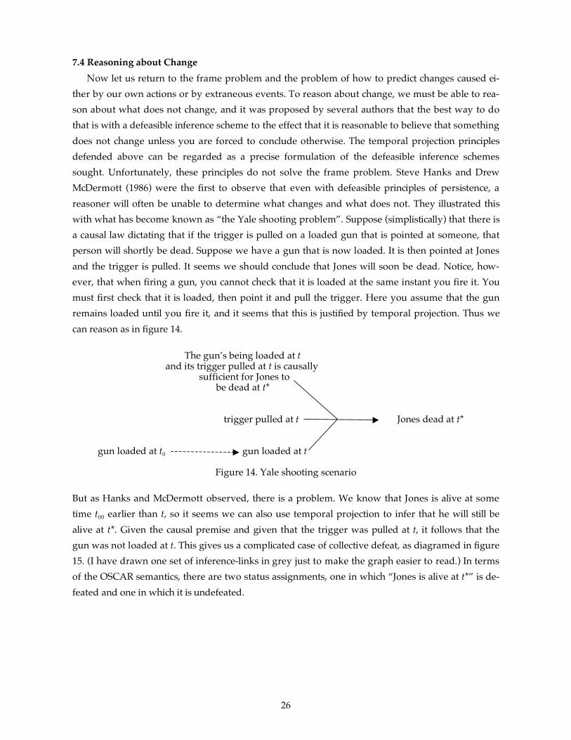
7.4 Reasoning about Change Now let us return to the frame problem and the problem of how to predict changes caused ei-ther by our own actions or by extraneous events. To reason about change, we must be able to rea-son about what does not change, and it was proposed by several authors that the best way to do that is with a defeasible inference scheme to the effect that it is reasonable to believe that something does not change unless you are forced to conclude otherwise. The temporal projection principles defended above can be regarded as a precise formulation of the defeasible inference schemes sought. Unfortunately, these principles do not solve the frame problem. Steve Hanks and Drew McDermott (1986) were the first to observe that even with defeasible principles of persistence, a reasoner will often be unable to determine what changes and what does not. They illustrated this with what has become known as “the Yale shooting problem”. Suppose (simplistically) that there is a causal law dictating that if the trigger is pulled on a loaded gun that is pointed at someone, that person will shortly be dead. Suppose we have a gun that is now loaded. It is then pointed at Jones and the trigger is pulled. It seems we should conclude that Jones will soon be dead. Notice, how-ever, that when firing a gun, you cannot check that it is loaded at the same instant you fire it. You must first check that it is loaded, then point it and pull the trigger. Here you assume that the gun remains loaded until you fire it, and it seems that this is justified by temporal projection. Thus we can reason as in figure 14.

The gun’s being loaded at t

and its trigger pulled at t is causally sufficient for Jones to

be dead at t*

trigger pulled at t Jones dead at t*

gun loaded at t0 gun loaded at t

Figure 14. Yale shooting scenario But as Hanks and McDermott observed, there is a problem. We know that Jones is alive at some time t00 earlier than t, so it seems we can also use temporal projection to infer that he will still be alive at t*. Given the causal premise and given that the trigger was pulled at t, it follows that the gun was not loaded at t. This gives us a complicated case of collective defeat, as diagramed in figure 15. (I have drawn one set of inference-links in grey just to make the graph easier to read.) In terms of the OSCAR semantics, there are two status assignments, one in which “Jones is alive at t*” is de-feated and one in which it is undefeated.

27

The gun’s being loaded at t

and its trigger pulled at t is causally sufficient for Jones to

be dead at t*

trigger pulled at t Jones dead at t*

gun loaded at t0 gun loaded at t

gun not loaded at t

Jones alive at t00 Jones alive at t*

Figure 15. Yale shooting problem The general form of this problem is common to cases of causal reasoning. We know that some proposition P is true at an initial time t0. We know that action A is performed at a subsequent time t, and we know that if P is still true at t then Q will become true at a later time t*. We want to infer de-feasibly that P will still be true at t, and hence that Q will become true at t*. This is the intuitively correct conclusion to draw. But temporal projection gives us a reason for thinking that because ~Q is true initially it will remain true at t*, and hence P was not true at t after all. The problem is to un-derstand what principles of reasoning enable us to draw the desired conclusion and avoid the col-lective defeat. When we reason about causal mechanisms, we think of the world as “unfolding” temporally, and changes only occur when they are forced to occur by what has already happened. In our ex-ample, when A is performed, nothing has yet happened to force a change in P, so we conclude de-feasibly that P remains true. But given the truth of P, we can then deduce that at a slightly later time, Q will become true. Thus when causal mechanisms force there to be a change, we conclude defeasibly that the change occurs in the later states rather than the earlier states. This seems to be part of what we mean by describing something as a causal mechanism. Causal mechanisms are sys-tems that force changes, where “force” is to be understood in the context of temporal unfolding.16 More precisely, when two temporal projections conflict because of a negative causal connection be-tween their conclusions, the projection to the conclusion about the earlier time takes precedence over the later projection. In other words, given the causal connection, the earlier temporal projec-tion provides a defeater for the later one. This can be captured as follows: Causal undercutting

16 This intuition is reminiscent of Shoham’s (1987) “logic of chronological ignorance”, although unlike Shoham, I pro-pose to capture the intuition without modifying the structure of the system of defeasible reasoning. This is also related to the proposal of Gelfond and Lifschitz (1993), and to the notion of progressing a database discussed in Lin and Reiter (1994 and 1995). This same idea underlies my analysis of counterfactual conditionals in Pollock (1979) and (1984).

28

If t0 < t < t* and t00 < t*, “P-at-t0 and A-at-t and [(P-at-t & A-at-t) is causally sufficient for Q at t*]” is an undercutting defeater for the inference by temporal projection from “~Q-at-t00” to “~Q-at-t*”.

Incorporating this undercutting defeater into figure 15 gives us figure 16. If we apply the OSCAR semantics to this inference graph, we find that there is just one status assignment, and in that status assignment the undercutting defeater is undefeated, and hence the temporal projection is defeated, so the conclusion that Jones is dead at t* is undefeated.

The gun’s being loaded at t

+ and its trigger pulled at t is causally sufficient for Jones to

be dead at t*

+ trigger pulled at t Jones dead at t* +

+ gun loaded at t trigger pulled at t and

+ gun loaded at t0 gun loaded at t and the gun’s being loaded at t +

and its trigger pulled at t is causally sufficient for

Jones to be dead at t* ⊗

Jones is alive at t*

– gun not loaded at t

+ Jones alive at t00 Jones alive at t* –

Figure 16. The solved Yale shooting problem

Technically, what makes this solution work is that the undercutting defeater is inferred from the premise of the earlier temporal projection (in this case, “The gun is loaded at t0”), not from the con-clusion of that projection. If we redraw the inference graph so that it is inferred instead from the conclusion, we get another case of collective defeat. However, it must be borne in mind that it is the initial temporal projection to which we are giving precedence, and not just its premise. This is sup-posed to be a way of adjudicating between conflicting temporal projections. So it cannot just be the premise of the earlier temporal projection that is relevant. This observation can be captured by ap-

pealing to the fact that undercutting defeaters are reasons for conclusions of the form (P⊗Q), and as

such they can be defeasible. In the case of causal undercutting, anything that defeats the earlier temporal projection should defeat the application of causal undercutting, thus reinstating the later temporal projection. For example, if we examined the gun at t0 and determined it was loaded, but then checked again before firing and the second time we looked it was not loaded, this defeats the temporal projection to the conclusion that the gun was loaded when fired. This is what I earlier

29

called “a discontinuity defeater”. In general, any defeater for the earlier temporal projection must also be a defeater for causal undercutting. We have noted two such defeaters, so we should have: Discontinuity defeat for causal undercutting

If t0 < t1 < t, “~P-at-t1” is an undercutting defeater for an application of causal undercutting.

Probabilistic defeat for causal undercutting “The probability of P-at-(t+1) given P-at-t is not high” is an undercutting defeater for an applica-tion of causal undercutting.

Thus the Yale Shooting Problem is solved. The same epistemic machinery that solves this prob-lem seems to handle causal reasoning in general. It is not quite right to describe this as a solution to the frame problem, because the frame problem arose on the assumption that all good reasoning is deductive. The frame problem was the problem of how to handle causal reasoning given that as-sumption. Once we embrace defeasible reasoning, the original frame problem goes away. There is no reason to think we should be able to handle causal reasoning in a purely deductive way. How-ever, the problem has a residue, namely, that of giving an account of how causal reasoning works. That is the problem I have tried to solve here. The solution has two parts — temporal projection and causal undercutting. In closing, it is worth noting that this reasoning is easily implemented in OSCAR. I invite the reader to download the OSCAR code from the OSCAR website17 and try it out on other problems.

8. Conclusions

The assumption that good reasoning must be deductively valid is seen to be wrong when we look carefully at the kinds of reasoning a sophisticated cognizer must be able to do. Defeasible rea-soning is the norm and deductive reasoning is the exception. Defeasible reasoning differs from de-ductive reasoning in that the reason-schemes employed in defeasible reasoning can have defeaters. A cognizer may produce a number of arguments, some of which defeat others. A semantics for de-feasible reasoning aims to tell us how it is determined which of those arguments are defeated and which are undefeated. A cognizer’s justified beliefs are then those that are supported by his unde-feated arguments. I described the OSCAR semantics for defeasible reasoning, and illustrated its ap-plication with a discussion of the frame problem.

9. Bibliography Chisholm, Roderick 1957 Perceiving. Ithaca: Cornell University Press. 17 http://oscarhome.soc-sci.arizona.edu/ftp/OSCAR-web-page/OSCAR.html.

30

1966 Theory of Knowledge, Englewood Cliffs, NJ: Prentice-Hall. Fodor, Jerry 2001 The Mind Doesn’t Work That Way, Cambridge, MA: MIT Press. Gelfond, Michael, and Lifschitz, Vladimir 1993 “Representing action and change by logic programs”, Journal of Logic Programming 17, 301-

322. Ginsberg, Matt 1987 Readings in Nonmonotonic Reasoning. Los Altos, CA: Morgan Kaufman. Hanks, Steve, and McDermott, Drew 1987 “Nonmonotonic logic and temporal projection”, Artificial Intelligence 33, 379-412. Harman, Gilbert 1973 Thought. Princeton: Princeton University Press. Hart, H. L. A. 1948 “The ascription of responsibility and rights”, Proceedings of the Aristotelian Society, 1948-9. Israel, David 1980 “What’s wrong with non-monotonic logic?” Proceedings of the First Annual National Confer-

ence on Artificial Intelligence. 99–101. Kyburg, Henry, Jr. 1961 Probability and the Logic of Rational Belief. Middletown, Conn.: Wesleyan University Press. 1970 “Conjunctivitis”, Marshall Swain (ed.), Induction, Accveptance, and Rational Belief. Dordrecht,

D. Reidel. Lin, Fangzhen, and Reiter, Raymond 1994 “How to progress a database (and why) I. Logical foundations.” In Proceedings of the Fourth

International Conference on Principles of Knowledge Representation (KR’94). 425-436. 1995 “How to progress a database II: The STRIPS connection.” IJCAI-95. 2001-2007. Makinson, D. and Schlechta, K. 1991 “Floating conclusions and zombie paths: Two deep difficulties in the ‘directly skeptical’ ap-

proach to inheritance nets”, Artificial Intelligence 48, 199-209. McCarthy, John 1980 “Circumscription — A form of non-monotonic reasoning”. Artificial Intelligence 13, 27-39,

171-172. 1986 “Applications of circumscription to formalizing common sense knowledge.” Artificial Intelli-

gence 26, 89-116. McCarthy, John, and Hayes, Patrick 1969 “Some philosophical problems from the standpoint of artificial intelligence”. In B. Metzer &

D. Michie (eds.), Machine Intelligence 4. Edinburgh: Edinburgh University Press. McDermott, Drew 1982 “A temporal logic for reasoning about processes and plans”, Cognitive Science 6, 101-155. McDermott, D., and Jon Doyle 1980 Non-monotonic logic I. Artificial Intelligence 13: 41-72.

31

Pollock, John 1967 “Criteria and our Knowledge of the Material World”, The Philosophical Review, 76, 28-60. 1970 “The structure of epistemic justification”, American Philosophical Quarterly, monograph series

4: 62-78. 1971 “Perceptual Knowledge”, Philosophical Review, 80, 287-319. 1974 Knowledge and Justification, Princeton University Press. 1979 Subjunctive Reasoning, D. Reidel. 1984 The Foundations of Philosophical Semantics, Princeton University Press. 1986 Contemporary Theories of Knowledge, Rowman and Littlefield. 1990 Nomic Probability and the Foundations of Induction, Oxford University Press. 1991 “Self-defeating arguments”. Minds and Machines 1 (1991), 367-392. 1995 Cognitive Carpentry, MIT Press. 1997 “Reasoning about change and persistence: a solution to the frame problem”, Nous 31, 143-

169. 1998 “Perceiving and reasoning about a changing world”, Computational Intelligence. 14, 498-562. 2002 “Defeasible reasoning with variable degrees of justification”, Artificial Intelligence 133, 233-

282. 2006 Thinking about Acting: Logical Foundations for Rational Decision Making. New York, Oxford. Pollock, John and Iris Oved 2006 “Vision, knowledge, and the mystery link”, with Iris Oved. In Philosophical Perspectives 19. Reiter, Raymond 1980 “A logic for default reasoning”. Artificial Intelligence 13, 81–132. Rescher, Nicholas 1977 Dialectics, Albany, NY: SUNY Albany Press. Sandewall, Erik 1972 “An approach to the frame problem and its implementation”. In B. Metzer & D. Michie

(eds.), Machine Intelligence 7. Edinburgh: Edinburgh University Press. Shoham, Yoav 1987 Reasoning about Change, MIT Press. Stalker, Douglas 1994 Grue: The New Riddle of Induction. Chicago, Open Court. Toulmin, Stephen 1958 The Place of Reason in Ethics, Cambridge.