Deep Semantic Classification for 3D LiDAR Data

Ayush Dewan Gabriel L. Oliveira Wolfram Burgard

Abstract— Robots are expected to operate autonomously indynamic environments. Understanding the underlying dynamiccharacteristics of objects is a key enabler for achieving thisgoal. In this paper, we propose a method for pointwise semanticclassification of 3D LiDAR data into three classes: non-movable,movable and dynamic. We concentrate on understanding thesespecific semantics because they characterize important informa-tion required for an autonomous system. To learn the distinctionbetween movable and non-movable points in the environment,we introduce an approach based on deep neural network andfor detecting the dynamic points, we estimate pointwise motion.We propose a Bayes filter framework for combining the learnedsemantic cues with the motion cues to infer the requiredsemantic classification. In extensive experiments, we compareour approach with other methods on a standard benchmarkdataset and report competitive results in comparison to theexisting state-of-the-art. Furthermore, we show an improvementin the classification of points by combining the semantic cuesretrieved from the neural network with the motion cues.

I. INTRODUCTION

One of the vital goals in mobile robotics is to develop asystem that is aware of the dynamics of the environment.If the environment changes over time, the system shouldbe capable of handling these changes. In this paper, wepresent an approach for pointwise semantic classification ofa 3D LiDAR scan into three classes: non-movable, movableand dynamic. Segments in the environment having non-zero motion are considered dynamic, a region which isexpected to remain unchanged for long periods of time isconsidered non-movable, whereas the frequently changingsegments of the environment is considered movable. Eachof these classes entail important information. Classifyingthe points as dynamic facilitates robust path planning andobstacle avoidance, whereas the information about the non-movable and movable points allows uninterrupted navigationfor long periods of time.

To achieve the desired objective, we use a ConvolutionalNeural Network (CNN) [19] for understanding the distinctionbetween movable and non-movable points. For our approach,we employ a particular type of CNNs called up-convolutionalnetworks [16]. They are fully convolutional architecturescapable of producing dense predictions for a high-resolutioninput. The input to our network is a set of three channel2D images generated by unwrapping 360◦ 3D LiDAR dataonto a spherical 2D plane and the output is the objectnessscore. Similarly, we estimate the dynamicity score for a pointby first calculating pointwise 6D motion using our previousmethod [6] and then comparing the estimated motion with

All authors are with the Department of Computer Science at the Univer-sity of Freiburg, Germany. This work has been supported by the EuropeanCommission under the grant numbers FP7-610532-SQUIRREL

Fig. 1. Semantic classification of a 3D LiDAR scan. Non-movable pointsare colored black. Points on parked vehicles, correctly classified as movableare shown in green, whereas the points on moving vehicles are classifiedas dynamic and are shown in blue.

the odometry to calculate the score. We combine the twoscores in a Bayes filter framework for improving the clas-sification especially for dynamic points. Furthermore, ourfilter incorporates previous measurements, which makes theclassification more robust. Fig. 1 shows the classificationresults of our method.

Other methods [18, 10] for similar semantic classificationhave been proposed for RGB images, however, a methodsolely relying on range data does not exist according to ourbest knowledge. For LiDAR data, separate methods existsfor both object detection [4, 13, 9, 3] and for distinguishingbetween static and dynamic objects in the scene [5, 15, 17].The two main differences between our method and the othermethods is that the output of our method is a pointwiseobjectness score, whereas other methods concentrate oncalculating object proposals and predict a bounding box forthe object. Since our objective is pointwise classification,the need for estimating a bounding box is alleviated as apointwise score currently suffices. The second difference isthat we utilize the complete 360◦ field of view (FOV) ofLiDAR for training our network in contrast to other methodswhich only use the points that overlap with the FOV of thefront camera.

The main contribution of our work is a method for seman-tic classification of a LiDAR scan for learning the distinctionbetween non-movable, movable and dynamic parts of thescene. A method for learning the same classes in LiDARscans has not been proposed before, even though differentmethods exists for learning other semantic information. Fortraining the neural network we use the KITTI object bench-mark [11]. We test our approach on the benchmark and thedataset by Moosmann and Stiller [15].

Rigid ow

Training

Input

Label

Bayes Filter

Objectness Score

Dynamic Score

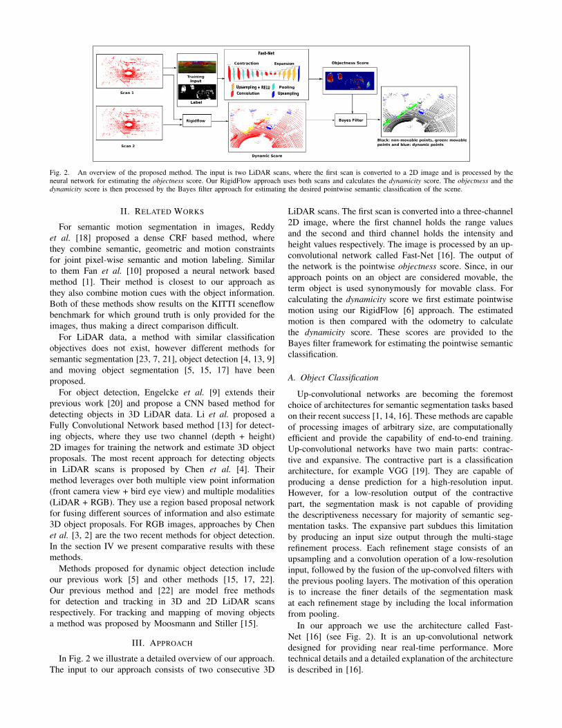
Fig. 2. An overview of the proposed method. The input is two LiDAR scans, where the first scan is converted to a 2D image and is processed by theneural network for estimating the objectness score. Our RigidFlow approach uses both scans and calculates the dynamicity score. The objectness and thedynamicity score is then processed by the Bayes filter approach for estimating the desired pointwise semantic classification of the scene.

II. RELATED WORKS

For semantic motion segmentation in images, Reddyet al. [18] proposed a dense CRF based method, wherethey combine semantic, geometric and motion constraintsfor joint pixel-wise semantic and motion labeling. Similarto them Fan et al. [10] proposed a neural network basedmethod [1]. Their method is closest to our approach asthey also combine motion cues with the object information.Both of these methods show results on the KITTI sceneflowbenchmark for which ground truth is only provided for theimages, thus making a direct comparison difficult.

For LiDAR data, a method with similar classificationobjectives does not exist, however different methods forsemantic segmentation [23, 7, 21], object detection [4, 13, 9]and moving object segmentation [5, 15, 17] have beenproposed.

For object detection, Engelcke et al. [9] extends theirprevious work [20] and propose a CNN based method fordetecting objects in 3D LiDAR data. Li et al. proposed aFully Convolutional Network based method [13] for detect-ing objects, where they use two channel (depth + height)2D images for training the network and estimate 3D objectproposals. The most recent approach for detecting objectsin LiDAR scans is proposed by Chen et al. [4]. Theirmethod leverages over both multiple view point information(front camera view + bird eye view) and multiple modalities(LiDAR + RGB). They use a region based proposal networkfor fusing different sources of information and also estimate3D object proposals. For RGB images, approaches by Chenet al. [3, 2] are the two recent methods for object detection.In the section IV we present comparative results with thesemethods.

Methods proposed for dynamic object detection includeour previous work [5] and other methods [15, 17, 22].Our previous method and [22] are model free methodsfor detection and tracking in 3D and 2D LiDAR scansrespectively. For tracking and mapping of moving objectsa method was proposed by Moosmann and Stiller [15].

III. APPROACH

In Fig. 2 we illustrate a detailed overview of our approach.The input to our approach consists of two consecutive 3D

LiDAR scans. The first scan is converted into a three-channel2D image, where the first channel holds the range valuesand the second and third channel holds the intensity andheight values respectively. The image is processed by an up-convolutional network called Fast-Net [16]. The output ofthe network is the pointwise objectness score. Since, in ourapproach points on an object are considered movable, theterm object is used synonymously for movable class. Forcalculating the dynamicity score we first estimate pointwisemotion using our RigidFlow [6] approach. The estimatedmotion is then compared with the odometry to calculatethe dynamicity score. These scores are provided to theBayes filter framework for estimating the pointwise semanticclassification.

A. Object Classification

Up-convolutional networks are becoming the foremostchoice of architectures for semantic segmentation tasks basedon their recent success [1, 14, 16]. These methods are capableof processing images of arbitrary size, are computationallyefficient and provide the capability of end-to-end training.Up-convolutional networks have two main parts: contrac-tive and expansive. The contractive part is a classificationarchitecture, for example VGG [19]. They are capable ofproducing a dense prediction for a high-resolution input.However, for a low-resolution output of the contractivepart, the segmentation mask is not capable of providingthe descriptiveness necessary for majority of semantic seg-mentation tasks. The expansive part subdues this limitationby producing an input size output through the multi-stagerefinement process. Each refinement stage consists of anupsampling and a convolution operation of a low-resolutioninput, followed by the fusion of the up-convolved filters withthe previous pooling layers. The motivation of this operationis to increase the finer details of the segmentation maskat each refinement stage by including the local informationfrom pooling.

In our approach we use the architecture called Fast-Net [16] (see Fig. 2). It is an up-convolutional networkdesigned for providing near real-time performance. Moretechnical details and a detailed explanation of the architectureis described in [16].

B. Training Input

For training our network we use the KITTI object bench-mark. The network is trained for classifying points on carsas movable. The input to our network are three channel 2Dimages and the corresponding ground truth labels. The 2Dimages are generated by projecting the 3D data onto a 2Dpoint map. The resolution of the image is 64× 870. TheKITTI benchmark provides ground truth bounding boxes forthe objects in front of the camera. To utilize the completeLiDAR information we use our tracking approach [5] for la-beling the objects that are behind the camera by propagatingthe bounding boxes from front of the camera.

1) Training: Our approach is modeled as a binary seg-mentation problem. We define a set of training imagesT = (Xn,Yn),n = 1, . . . ,N, where Xn = {xk,k = 1, . . . , |Xn|}is a set of pixels in an example input image and Yn ={yk,k = 1, . . . , |Yn|} is the corresponding ground truth, whereyk = {0,1}. The activation function of our model is definedas f (xk,θ), where θ is our network model parameters.The network learns the features by minimizing the cross-entropy(softmax) loss in Eq. (1) and the final weights θ ∗ areestimated by minimizing the loss over all the pixels as shownin Eq. (2).

L(p,q) =− ∑c∈{0,1}

pc logqc (1)

θ∗ = argmin

θ

N×|Xn|

∑k=1

L( f (xk,θ) ,yk) (2)

We perform a multi-stage training, by using one singlerefinement at a time. The process consists of initializing thecontractive side with the VGG weights. After that the multi-stage training begins and each refinement is trained until wereach the final stage that uses the first pooling layer.

We use Stochastic Gradient Descent with momentum(0.99) as the optimizer, a mini batch of size one and a fixedlearning rate of 1e−6. Since the labels in our problem areunbalanced because the majority of the points belong tothe non-movable class, we incorporate class balancing asexplained by Eigen and Fergus [8].

The output of the network is a pixel wise score akc for

each class c. The required objectness score ξ k ∈ [0,1] fora point k is the posterior class probability for the movableclass.

ξk =

exp(ak1)

exp(ak1)+ exp(ak

0)(3)

C. RigidFlow

In our previous work [6], we proposed a method forestimating pointwise motion in LiDAR scans. The input toour method are two consecutive scans and the output is thecomplete 6D motion for every point in the scan. We representthe problem using a factor graph G = (Φ,T ,E ) with twonode types: factor nodes φ ∈ Φ and state variables nodesτk ∈T . Here, E is the set of edges connecting Φ and statevariable nodes T .

The factor graph describes the factorization of the function

φ(T ) = ∏i∈Id

φd(τi) ∏l∈Np

φp(τi,τ j), (4)

where T is the following rigid motion field:

T = {τk | τk ∈ SE(3),k = 1, . . . ,K} (5)

{φd ,φp} ∈ φ are two types of factor nodes describing theenergy potentials for the data term and regularization termrespectively. The term Id is the set indices corresponding tokeypoints in the first frame and Np = {〈1,2〉,〈2,3〉, . . . ,〈i, j〉}is the set containing indices of neighboring vertices. Thedata term, defined only for keypoints is used for estimatingmotion, whereas the regularization term asserts that theproblem is well posed and spreads the estimated motion tothe neighboring points. The output of our method is a denserigid motion field T ∗, the solution of the following energyminimization problem:

T ∗ = argminT

E(T ), (6)

where the energy function is:

E(T ) =− lnφ(T ) (7)

A more detailed explanation of the method is presented byDewan et al. [6].

D. Bayes Filter for Semantic Classification

The rigid flow approach estimates pointwise motion, how-ever it does not provide the semantic level information. Tothis end, we propose a Bayes filter method for combiningthe learned semantic cues from the neural network with themotion cues for classifying a point as non-movable, movableand dynamic. The input to our filter is the estimated 6Dmotion, odometry and the objectness score.

The objectness score from the neural network is sufficientfor classifying points as movable and non-movable, however,we still include this information in filter framework for thefollowing two reasons:• Adding object level information improves the results for

dynamic classification because a point belonging to anon-movable object has infinitesimal chance of beingdynamic, in comparison to a movable object.

• Having a filter over the classification from the network,allows filtering of wrong classification results by usingthe information from the previous frames.

For every point Pkt ∈ R3 in the scan, we define a state

variable xt = {dynamic, movable, non-movable}.The objective is to estimate the belief of the current statefor a point Pk

t .

Bel(xkt ) = p(xk

t | xk1:t−1,τ

k1:t ,ξ

k1:t ,o

kt ) (8)

The current belief depends on the previous states xk1:t−1,

motion measurements τk1:t , object measurements ξ k

1:t anda Bernoulli distributed random variable ok

t . This variablemodels the object information, where ok

t = 1 means that a

point belongs to an object and therefore it is movable. For thenext set of equations we skip the superscript k that representsthe index of a point.

Bel(xt) = p(xt | x1:t−1,τ1:t ,ot ,ξ1:t) (9)

= η p(τt ,ot | xt ,ξ1:t)∫

p(xt | xt−1)Bel(xt−1)dxt−1 (10)

= η p(τt | xt)p(ot | xt ,ξ1:t)∫

p(xt | xt−1)Bel(xt−1)dxt−1

(11)

In Eq. (10) we show the simplification of the Eq. (8) usingthe Bayes rule and the Markov assumption. The likelihoodfor the motion measurement is defined in Eq. (12).

p(τt | xt) = N (τt ; τt ,Σ) (12)

It compares the expected measurement τt with the observedmotion. In our case the expected motion is the odometrymeasurement. The output of the likelihood function is therequired dynamicity score.

In Eq. (11) we assume the independence between theestimated motion and the object information. To calculatethe object likelihood we first update the value of the randomvariable ot by combining the current objectness score ξtwith the previous measurements in a log-odds formulation(Eq. (13)).

l(ot | ξ1:t) = l(ξt)+ l(ot | ξ1:t−1)− l(o0) (13)

The first term on the right side incorporates the currentmeasurement, the second term is the recursive term whichdepends on the previous measurements and the last termis the initial prior. In our experiments, we set o0 = 0.2because we assume that the scene predominately containsnon-moving objects.

p(ot | xt ,ξ1:t) =

p(¬ot | ξ1:t) if xt = non-movable

p(ot | ξ1:t) if xt = movable

s · p(ot | ξ1:t) if xt = dynamic(14)

The object likelihood model is shown in Eq. (14). Asthe neural network is trained to predict the non-movableand movable class, the first two cases in Eq. (14) arestraightforward. For the case of dynamic object, we scalethe prediction of movable class by a factor s ∈ [0,1] sinceall the dynamic objects are movable. This scaling factorapproximates the ratio of number of dynamic objects inthe scene to the number of movable objects. This ratio isenvironment dependent for instance on a highway, value ofs will be close to 1, since most of movable objects will bedynamic. For our experiments, through empirical evaluation,we chose the value of s = 0.6.

IV. RESULTS

To evaluate our approach we use the dataset from theKITTI object benchmark and the dataset provided by Moos-mann and Stiller [15]. The first dataset provides object anno-tations but does not provide the labels for moving objects and

for the second dataset we have the annotations for movingobjects [5]. Therefore to analyze the classification of movableand non-movable points we use the KITTI object benchmarkand use the second dataset for examining the classification ofdynamic points. For all the experiments, Precision and Recallare calculated by varying the confidence measure of theprediction. For object classification the confidence measureis the objectness score and for dynamic classification theconfidence measure is the output of the Bayes filter approach.The reported F1-score is always the maximum F1-scorefor the estimated Precision Recall curves and the reportedprecision and recall corresponds to the maximum F1-score.

A. Object Classification

The KITTI object benchmark provides 7481 annotatedscans. Out of these scans we chose 1985 scans and createda dataset of 3789 scans by tracking the labeled objects.The implementation of Fast-Net is based on a deep learningtoolbox Caffe [12]. The network was trained and tested on asystem containing an NVIDIA Titan X GPU. For testing, weuse the same validation set as mentioned by Chen et al. [4].

We provide quantitative analysis of our method for bothpointwise prediction and object-wise prediction. For object-wise prediction we compare with these methods [3, 2, 13, 4].Output for all of these methods is bounding boxes for thedetected objects. A direct comparison with these methods isdifficult since output of our method is pointwise prediction,however, we still make an attempt by creating boundingboxes out of our pointwise prediction as a post-processingstep. We project the predictions from 2D image space toa 3D point cloud and then estimate 3D bounding boxesby clustering points belonging the to same surface as oneobject [6].

TABLE IOBJECT CLASSIFICATION AP3D

Method Data IoU=0.5 timeEasy Moderate HardMono3D [3] Mono 25.19 18.2 15.52 4.2s

3DOP [2] Stereo 46.04 34.63 30.09 3sVeloFCN [13] LiDAR 67.92 57.57 52.56 1s

MV3D [4] LiDAR (FV) 74.02 62.18 57.61 -MV3D [4] LiDAR

(FV+BV)95.19 87.65 80.11 0.3s

MV3D [4] LiDAR(FV+BV+Mono)

96.02 89.05 88.38 0.7s

Ours LiDAR 95.31 71.87 70.01 0.07s

TABLE IIPOINTWISE VERSUS OBJECT-WISE PREDICTION

Method Recall Recall (easy) Recall (moderate) Recall (hard)pointwise 81.29 84.79 71.07 68.10

object-wise 60.47 87.91 48.44 46.80

For object-wise precision, we follow the KITTI benchmarkguidelines and report average precision for easy, moderateand hard cases. We compare the average precision for 3Dbounding boxes AP3D and the computational time with the

Fig. 4. A LiDAR scan from Scenario-B. Points classified as non-movable are shown in black, points classified as movable are shown in green and pointsclassified as dynamic are shown in blue.

TABLE IIIOBJECT CLASSIFICATION F1-SCORE

Method F1 Score Precision RecallSeg-Net 69.83 85.27 59.12

Without Class Balancing 78.14 76.73 79.60Ours(Fast-Net) 80.16 79.06 81.29

0 0.2 0.4 0.6 0.8 10

0.2

0.4

0.6

0.8

1

Recall

Pre

cis

ion

Ours (Fast-Net)

Without weight balancing

Seg-Net

0 0.2 0.4 0.6 0.8 10

0.2

0.4

0.6

0.8

1

Recall

Pre

cis

ion

Experiment 1

Experiment 2

Experiment 3

Fig. 3. Left: Precision Recall curves for object classification. Right:Precision recall curves for dynamic classification. Experiment 1 involvesusing the proposed Bayes filter approach, in experiment 2, the objectinformation is not updated recursively and for the experiment 3, only motioncues are used for classification.

other methods in Tab. I. Our method outperforms the firstthree methods and an instance of the last method (frontview) in terms of AP3D. The computational time for ourmethod includes the pointwise prediction on a GPU andobject-wise prediction on CPU. The time reported for all themethods in Tab. I is the processing time on GPU. The CPUprocessing time for object-wise prediction of our methodis 0.30s. Even though performance of our method is notcomparable with the two cases where LiDAR front view (FV)data is combined with bird eye view (BV) and RGB data,the computational time for our method is nearly 10× faster.

In Tab. II we report the pointwise and object-wise recallfor the complete test data and for the three difficultylevels. The object level recall correspond to the AP3Dresults in Tab. I. The reported pointwise recall is theactual evaluation of our method. The decrease in recallfrom pointwise prediction to object-wise is predominantlyfor moderate and hard case because objects belongingto these difficulty levels are often far and occludedtherefore discarded during object clustering. The decreasein performance from pointwise to object-wise predictionshould not be seem as a drawback of our approach sinceour main focus is to estimate precise and robust pointwise

Fig. 5. Bayes filter correction for dynamic class. The image on the leftis a visual representation of the dynamicity score and right image is theclassification results, where non-movable points are shown black, movablepoints are shown in green and dynamic points are shown in blue. The colorbar shows the range of colors for the score ranging from 0 to 1. Themisclassified points in the left image (left corner) are correctly classifiedas non-movable after the addition of the object information.

Fig. 6. Bayes filter correction for movable class. The image on the leftis a visualization of objectness score, where blue points corresponds tomovable class. The purple rectangle highlights movable points with lowscore. The image in the middle and right shows classification of Bayes filter,where green points correspond to movable class. For the middle image,the object information was not recursively updated (second experiment)in the filter framework. For the right image we use the proposed Bayesfilter approach (experiment 1). The points having low score is correctlyclassified as movable since the filter considers the current measurement andthe previous measurements, which shows the significance of updating thepredictions from the neural network within the filter.

prediction required for the semantic classification.

We show the Precision Recall curves for pointwise objectclassification in Fig. 3 (right). Our method outperformsSeg-Net and we report an increase in F1-score by 12%(see Tab. III). This network architecture was used by Fanet al. [10] in their approach. To highlight the significance ofclass balancing, we trained a neural network without classbalancing. Inclusion of this information increases the recallpredominantly at high confidence values (see Fig. 3).

B. Semantic Classification

For the evaluation of semantic classification we use apublicly available dataset [15]. The dataset consists of twosequences: Scenario-A and Scenario-B.

TABLE IVDYNAMIC CLASSIFICATION F1-SCORE

Method Scenario A Scenario BF1-score Precision Recall F1-score Precision Recall

Experiment 1 82.43 87.48 77.9 72.24 76.29 68.60Experiment 2 84.44 83.85 84.9 71.48 75.83 67.66Experiment 3 81.40 72.77 92.34 63.89 59.46 69.62

We report the results for the dynamic classification forthree different experiments. For first experiment we use theapproach discussed in Sec. III-D. In the second experi-ment, we skip the step of updating the object information(see Eq. (13)) and only use the current objectness scorewithin the filter framework. For the final experiment, theclassification of dynamic points rely solely on motion cues.

We show the Precision Recall curves for classification ofdynamic points for all the three experiments for Scenario-Ain Fig. 3 (right). The PR curves illustrates that the objectinformation affects the sensitivity (recall) of the dynamicclassification, for instance when the classification is basedonly on motion cues (red curve), recall is better among all thethree cases. With the increase in object information sensitiv-ity decreases, thereby causing a decrease in recall. In Tab. IVwe report the F1-score for all the three experiments on boththe datasets. For both the scenarios, F1-score increases afteradding the object information which shows the significanceof leveraging the object cues in our framework. In Fig. 5,we show a visual illustration for this case. We would alsolike to emphasize that the affect of including the predictionsfrom the neural network in the filter is not only restrictedto classification of dynamic points. In Fig. 6, we show theimpact of our proposed filter framework on the classificationof movable points.

V. CONCLUSION

In this paper, we present an approach for pointwise se-mantic classification of a 3D LiDAR scan. Our approachuses an up-convolutional neural network for understandingthe difference between movable and non-movable pointsand estimates pointwise motion for inferring the dynamicsof the scene. In our proposed Bayes filter framework, wecombine the information retrieved from the neural networkwith the motion cues to estimate the required pointwise se-mantic classification. We analyze our approach on a standardbenchmark and report competitive results in terms for both,average precision and the computational time. Furthermore,through our Bayes filter framework we show the benefitsof combining learned semantic information with the motioncues for precise classification. For both the datasets weachieve a better F1-score. We also show that introducingthe object cues in the filter improves the classification ofmovable points.

REFERENCES[1] Vijay Badrinarayanan, Alex Kendall, and Roberto Cipolla. Seg-

net: A deep convolutional encoder-decoder architecture for imagesegmentation. arXiv preprint arXiv: 1511.00561, 2015. URLhttp://arxiv.org/abs/1511.00561.

[2] Xiaozhi Chen, Kaustav Kundu, Yukun Zhu, Andrew G Berneshawi,Huimin Ma, Sanja Fidler, and Raquel Urtasun. 3d object proposals

for accurate object class detection. In Advances in Neural InformationProcessing Systems, pages 424–432, 2015.

[3] Xiaozhi Chen, Kaustav Kundu, Ziyu Zhang, Huimin Ma, Sanja Fidler,and Raquel Urtasun. Monocular 3d object detection for autonomousdriving. In IEEE Conference on Computer Vision and PatternRecognition (CVPR), 2016.

[4] Xiaozhi Chen, Huimin Ma, Ji Wan, Bo Li, and Tian Xia. Multi-view3d object detection network for autonomous driving. arXiv preprintarXiv:1611.07759, 2016.

[5] Ayush Dewan, Tim Caselitz, Gian Diego Tipaldi, and Wolfram Bur-gard. Motion-based detection and tracking in 3d lidar scans. In IEEEInternational Conference on Robotics and Automation (ICRA), 2016.

[6] Ayush Dewan, Tim Caselitz, Gian Diego Tipaldi, and Wolfram Bur-gard. Rigid scene flow for 3d lidar scans. In IEEE/RSJ InternationalConference on Intelligent Robots and Systems (IROS), 2016.

[7] David Dohan, Brian Matejek, and Thomas Funkhouser. Learninghierarchical semantic segmentations of lidar data. In 3D Vision (3DV),2015 International Conference on, pages 273–281. IEEE, 2015.

[8] David Eigen and Rob Fergus. Predicting depth, surface normals andsemantic labels with a common multi-scale convolutional architecture.In Proceedings of the IEEE International Conference on ComputerVision, pages 2650–2658, 2015.

[9] Martin Engelcke, Dushyant Rao, Dominic Zeng Wang, Chi Hay Tong,and Ingmar Posner. Vote3deep: Fast object detection in 3d pointclouds using efficient convolutional neural networks. arXiv preprintarXiv:1609.06666, 2016.

[10] Qiu Fan, Yang Yi, Li Hao, Fu Mengyin, and Wang Shunting. Semanticmotion segmentation for urban dynamic scene understanding. In Au-tomation Science and Engineering (CASE), 2016 IEEE InternationalConference on, pages 497–502. IEEE, 2016.

[11] Andreas Geiger, Philip Lenz, and Raquel Urtasun. Are we readyfor autonomous driving? the kitti vision benchmark suite. In IEEEConference on Computer Vision and Pattern Recognition (CVPR),2012.

[12] Y. Jia, E. Shelhamer, J. Donahue, S. Karayev, J. Long, R. Girshick,S. Guadarrama, and T. Darrell. Caffe: Convolutional architecture forfast feature embedding. arXiv preprint arXiv:1408.5093, 2014.

[13] Bo Li, Tianlei Zhang, and Tian Xia. Vehicle detection from 3d lidarusing fully convolutional network. arXiv preprint arXiv:1608.07916,2016.

[14] Jonathan Long, Evan Shelhamer, and Trevor Darrell. Fully convo-lutional networks for semantic segmentation. IEEE Conference onComputer Vision and Pattern Recognition (CVPR), 2015.

[15] Frank Moosmann and Christoph Stiller. Joint self-localization andtracking of generic objects in 3d range data. In IEEE InternationalConference on Robotics and Automation (ICRA), 2013.

[16] G. L. Oliveira, W. Burgard, and T. Brox. Efficient deep models formonocular road segmentation. In IEEE/RSJ International Conferenceon Intelligent Robots and Systems (IROS), 2016.

[17] Francois Pomerleau, Philipp Krusi, Francis Colas, Paul Furgale, andRoland Siegwart. Long-term 3d map maintenance in dynamic environ-ments. In IEEE International Conference on Robotics and Automation(ICRA), 2014.

[18] N Dinesh Reddy, Prateek Singhal, and K Madhava Krishna. Semanticmotion segmentation using dense crf formulation. In Proceedings ofthe 2014 Indian Conference on Computer Vision Graphics and ImageProcessing, page 56. ACM, 2014.

[19] Karen Simonyan and Andrew Zisserman. Very deep convolutionalnetworks for large-scale image recognition. International Conferenceon Learning Representations (ICLR), 2015.

[20] Dominic Zeng Wang and Ingmar Posner. Voting for voting in onlinepoint cloud object detection. In Robotics: Science and Systems, 2015.

[21] Dominic Zeng Wang, Ingmar Posner, and Paul Newman. What couldmove? finding cars, pedestrians and bicyclists in 3d laser data. InRobotics and Automation (ICRA), 2012 IEEE International Conferenceon, pages 4038–4044. IEEE, 2012.

[22] Dominic Zeng Wang, Ingmar Posner, and Paul Newman. Model-free detection and tracking of dynamic objects with 2d lidar. TheInternational Journal of Robotics Research (IJRR), 34(7), 2015.

[23] Allan Zelener and Ioannis Stamos. Cnn-based object segmentation inurban lidar with missing points. In 3D Vision (3DV), 2016 FourthInternational Conference on, pages 417–425. IEEE, 2016.