deep-sea research ii€¦ · surface chlorophyll as the primary variable of interest; (2) con-...

Deep-Sea Research II ] (]]]]) ]]]–]]]

Contents lists available at SciVerse ScienceDirect

Deep-Sea Research II

0967-06

http://d

n Corr

E-m

Pleaslocal

journal homepage: www.elsevier.com/locate/dsr2

Satellite views of Pacific chlorophyll variability: Comparisons to physicalvariability, local versus nonlocal influences and links to climate indices

Andrew C. Thomas a,n, P. Ted Strub b, Ryan A. Weatherbee a, Corinne James b

a School of Marine Sciences, 5706 Aubert Hall, University of Maine, Orono, ME 04469, USAb College of Earth, Ocean and Atmospheric Sciences, Oregon State University, Corvallis, OR, USA

a r t i c l e i n f o

Keywords:

Pacific

Chlorophyll

Sea level

Surface temperature

Eastern boundary currents

Climate indices

Satellite data

45/$ - see front matter & 2012 Elsevier Ltd. A

x.doi.org/10.1016/j.dsr2.2012.04.008

esponding author. Tel.: þ1 207 581 4335; fax

ail address: [email protected] (A.C. Thomas

e cite this article as: Thomas, A.C.,versus nonlocal influences and link

a b s t r a c t

Concurrent satellite-measured chlorophyll (CHL), sea surface temperature (SST), sea level anomaly

(SLA) and model-derived wind vectors from the 13þ year SeaWiFS period September 1997–December

2010 quantify time and space patterns of phytoplankton variability and its links to physical forcing in

the Pacific Ocean. The CHL fields are a metric of biological variability, SST represents vertical mixing and

motion, often an indicator of nutrient availability in the upper ocean, SLA is a proxy for pycnocline

depths and surface currents while vector winds represent surface forcing by the atmosphere and

vertical motions driven by Ekman pumping. Dominant modes of variability are determined using

empirical orthogonal functions (EOFs) applied to a nested set of domains for comparison: over the

whole basin, over the equatorial corridor, over individual hemispheres at extra-tropical latitudes

(4201) and over eastern boundary current (EBC) upwelling regions. Strong symmetry exists between

hemispheres and the EBC regions, both in seasonal and non-seasonal variability. Seasonal variability is

strongest at mid latitudes but non-seasonal variability, our primary focus, is strongest along the

equatorial corridor. Non-seasonal basin-scale variability is highly correlated with equatorial signals and

the strongest signal across all regions in the study period is associated with the 1997–1999 ENSO cycle.

Results quantify the magnitude and geographic pattern with which dominant basin-scale signals are

expressed in extra-tropical regions and the EBC upwelling areas, stronger in the Humboldt Current than

in the California Current. In both EBC regions, wind forcing has weaker connections to non-seasonal

CHL variability than SST and SLA, especially at mid and lower latitudes. Satellite-derived dominant

physical and biological patterns over the basin and each sub-region are compared to indices that track

aspects of climate variability in the Pacific (the MEI, PDO and NPGO). We map and compare the local

CHL footprint associated with each index and those of local wind stress curl, showing the dominance in

most areas of the MEI and its similarity to the PDO. Principal estimator patterns quantify the linkage

between dominant modes of forcing variability (wind, SLA and SST) and CHL response, comparing local

interactions within EBC regions with those imposed by equatorial signals and mapping equatorial

forcing on extra-tropical CHL variability.

& 2012 Elsevier Ltd. All rights reserved.

1. Introduction

The climatological pattern of surface phytoplankton biomassover the Pacific basin (Fig. 1) reflects dominant patterns of heating,wind stress and stratification that control the flux of subsurfacenutrients into the euphotic zone. Seasonal variability about thispattern is dominated by mid-latitude shifts in the location of thetransition zone separating oligotrophic subtropical gyre waters frommore productive waters at higher latitudes (Longhurst, 1995;Vantrepotte and Melin, 2009; Yoder and Kennelly, 2003). Elsewhere,responses to interannual forcing, often of equatorial origin such as

ll rights reserved.

: þ1 207 581 4388.

).

et al., Satellite views of Pacs to climate indices. Deep-S

the El Nino Southern Oscillation (ENSO), can be of similar magnitudeor larger than local seasonal cycles (e.g., Chavez et al., 1999;Martinez et al., 2009; Vantrepotte and Melin, 2011; Yoder andKennelly, 2003), transmitted through atmospheric teleconnections(e.g., Chhak and DiLorenzo, 2007; Schwing et al., 2010) and oceanicpathways (e.g., Hormazabal et al., 2001; Strub and James, 2002c).Along the eastern basin margins, the biologically productiveCalifornia and Humboldt eastern boundary current (EBC) upwellingsystems respond rapidly and strongly to basin scale signals imposedfrom lower latitudes (Carr et al., 2002; Kahru and Mitchell, 2000) aswell as higher latitudes (Freeland et al., 2003; Wheeler et al., 2003).Such EBC variability is superimposed on more locally controlledvariability driven by latitudinally modulated seasonal wind forcingand heating (Bakun and Nelson, 1991; Thomas et al., 2001b). Theenergetic structure and relatively strong time and space gradients of

ific chlorophyll variability: Comparisons to physical variability,ea Res. II (2012), http://dx.doi.org/10.1016/j.dsr2.2012.04.008

www.elsevier.com/locate/dsr2

www.elsevier.com/locate/dsr2

dx.doi.org/10.1016/j.dsr2.2012.04.008

dx.doi.org/10.1016/j.dsr2.2012.04.008

dx.doi.org/10.1016/j.dsr2.2012.04.008

mailto:[email protected]

dx.doi.org/10.1016/j.dsr2.2012.04.008

dx.doi.org/10.1016/j.dsr2.2012.04.008

dx.doi.org/10.1016/j.dsr2.2012.04.008

dx.doi.org/10.1016/j.dsr2.2012.04.008

Fig. 1. The study area showing major geographic locations, climatological mean chlorophyll concentrations and the geographic boundaries of sub-regions (equatorial

corridor 7201, North Pacific and South Pacific 201–601, California and Humboldt Currents) among which regional variability is compared. Marginal seas were not included

in the analysis.

A.C. Thomas et al. / Deep-Sea Research II ] (]]]]) ]]]–]]]2

EBCs make them logical regions to examine oceanic responses toclimate-related signals.

Satellite data provide the most systematic views of coupledbiological–physical interannual variability over large spatialscales. Over the Pacific, linkages between chlorophyll (CHL) andphysical variability characterized by sea surface temperature(SST) and sea level anomaly (SLA) have been described for specificareas and/or time periods (e.g., Carr et al., 2002; Murtuguddeet al., 1999; Signorini and McClain, 2012; Wilson and Adamec,2001). Other works (Martinez et al., 2009; Vantrepotte and Melin,2011) extend these views, quantifying linkages between CHL, SSTand climate-related signals over the entire Pacific. Symmetrybetween SST patterns in each hemisphere has been shown(Shakun and Shaman, 2009), however, the symmetry of coupledbiological–physical patterns in each hemisphere and the extent towhich such basin-scale variability is reflected in EBC systemsremains less well described. Here, we build upon these previousefforts; examining the full SeaWiFS mission period (13þ years)and concurrent SST and SLA satellite data for dominant patternsover the whole basin and various sub-regions of the Pacific Ocean.We describe the relative symmetry of patterns in the northernand southern hemispheres, the projection of equatorial and basin-scale patterns into the EBC regions and the relationship betweensatellite-measured variability and three Pacific climate indices.We then quantify local EBC biological–physical coupling, con-trasting it with forcing of EBC regions from the equatorial zone.

Patterns of atmospheric and hydrographic variability along thePacific equatorial corridor and their local biological responseare dominated by interannual variability associated with ENSOevents with periods of two to seven years (Philander, 1999),effectively tracked by the multivariate ENSO index (Wolter andTimlin, 1998). The signature of ENSO is the leading mode of SSTvariability in the Pacific (Deser et al., 2010). The oceanic biologicalimplications of ENSO variability are evident throughout thePacific and up to global scales (Chavez et al., 2011; Martinezet al., 2009). Within the Pacific, ENSO signals have their mostdirect extra-tropical impact in the two Pacific eastern boundarycurrents (EBCs), where eastward propagating equatorial Kelvinwaves have a direct connection into the Humboldt Current as aresult of coastline shape and proximity and less direct but stillclear connections into the California Current (Strub and James,

Please cite this article as: Thomas, A.C., et al., Satellite views of Paclocal versus nonlocal influences and links to climate indices. Deep-S

2002a). These excite poleward propagating coastal-trappedwaves. In these EBCs, the arrival of elevated sea levels, a deeperupper mixed layer and warmer, nutrient-poor surface conditionsduring an El Nino event means wind-driven coastal upwellingdoes not bring nutrient-rich water to the surface, leading tosharply reduced coastal phytoplankton biomass (Kahru andMitchell, 2002; Ulloa et al., 2001).

On multi-decadal timescales in the North Pacific, the PacificDecadal Oscillation (Mantua and Hare, 2002) serves as an index ofoceanic climate variability. Defined as the dominant mode ofsurface temperature variability north of 201N, the PDO is theNorth Pacific response to atmospheric forcing by the winterstrength of the Aleutian low (Bond and Harrison, 2000) and isconnected to ENSO forcing (Di Lorenzo et al., 2010; Shakunand Shaman, 2009). The PDO is strongly correlated with mergedSST–CHL non-seasonal variability over the Pacific basin (Martinezet al., 2009) and linked to biological variability across multipletrophic levels (Anderson and Paitt, 1999; Cloern et al., 2010).Thomas et al. (2009) show positive correlations over a 7-yearperiod for coastal chlorophyll in the northern California Current(41–481N) and off Baja California 28–311N. The second mode ofNorth Pacific SST and SLA variability, the North Pacific GyreOscillation (Di Lorenzo et al., 2008) describes the relative strengthof gyre circulation and has correlations with salinity and nutrientconcentrations in the North Pacific, phytoplankton biomass in thesouthern California Current, and is positively correlated to coastalchlorophyll off the Pacific Northwest and off Baja California(Thomas et al., 2009). It also has links to ENSO forcing (DiLorenzo et al., 2010). In the South Pacific, the footprint of thePDO and the NPGO on biological variability remains poorlydescribed, but both appear to have correlations to coastal CHLin the Humboldt Current, at least at specific latitudes (Thomaset al., 2009).

Our analyses are shaped by three perspectives: (1) use ofsurface chlorophyll as the primary variable of interest; (2) con-sideration of the Pacific Basin but with its two EBCs as theprimary regions of interest; and (3) use of consistently processedsatellite data where possible, in order to obtain a ‘‘synoptic’’ viewof biophysical interactions over the widest and most uniformlysampled range of spatial scales possible. The SeaWiFS instrumentprovides over 13 years of basin-scale coverage of phytoplankton


dx.doi.org/10.1016/j.dsr2.2012.04.008

dx.doi.org/10.1016/j.dsr2.2012.04.008

dx.doi.org/10.1016/j.dsr2.2012.04.008

A.C. Thomas et al. / Deep-Sea Research II ] (]]]]) ]]]–]]] 3

biomass. Temporally coincident missions measured physical pro-cesses that potentially modulate phytoplankton patterns: SST (ametric of surface stratification, mixing and nutrient availability)and SLA (a metric of pycnocline depth and current structure). Weaugment these with model wind stress (wind stress curl: thedriver of Ekman pumping/suction and alongshore wind stress: thedriver of coastal upwelling). Against a background of betterknown seasonal CHL variability (Vantrepotte and Melin, 2009;Yoder et al., 2010), our objectives are to relate satellite-derivedfields of CHL to fields of SLA, SST and wind stress in the PacificBasin in order to: (1) contrast the synoptic modes of variability ofCHL with physical variables, including the degree of symmetrybetween hemispheres; (2) relate basin-scale signals to those of thetwo Pacific EBC regions, comparing them to local forcing; and(3) relate satellite-derived statistical modes to three indexes ofclimate variability, the MEI, PDO and the NPGO. For completeness,we recognize our study areas have links to variability in the westernPacific basin (Miller et al., 2004) that are not addressed here.

2. Data and methods

SeaWiFS monthly-averaged CHL over the duration of themission (September 1997–December 2010) were obtained fromthe NASA ocean color server. CHL values are the standard NASAchlorophyll algorithm (O’Reilly et al., 1998), reprocessing versionR2010. Instrument difficulties create four data gaps of 2–4months duration in 2008 and 2009. At latitudes 4�501, fewdata are available during hemisphere winter months due todarkness. We work with log transformed CHL values, consistentwith previous work showing their underlying distribution(Campbell, 1995). Even in the monthly means, CHL retrievals atsome pixels in this data set have some suspiciously high values,likely a result of localized failures in atmospheric correction,cloud edge effects and/or bio-optical algorithm failure in turbidwater, creating noisy fields. We reduce this noise in a series ofsteps, cognizant of our focus on longer time/space scale signals.Values greater than 30 mg m�3 were flagged as missing. Datawere then log10 transformed and at each location values greaterthan the climatological mean plus two standard deviationswere also flagged as missing. Data were transformed back intochlorophyll space and a 3�3 median spatial operator was thenpassed over each monthly field twice, and then transformedback into log10 units and the climatological mean at each locationwas removed. We use two time series, (log transformed) CHLconcentrations with zero mean at each location (retainingseasonality) and monthly anomalies created by subtracting theclimatological months from each year at each location.

Maps of 1/4 degree SLA gridded from multiple satellites wereobtained from AVISO (http://www.aviso.oceanobs.com). For Sep-tember 1997–November 2010, monthly averages were createdfrom available weekly fields of the AVISO Updated Delayed Timesea level anomaly product. We extended the SLA time series onemonth through December 2010 using ‘‘near real time’’ SLA datafor consistency with the other time series. For June 2010 throughDecember 2010, daily fields of the AVISO Daily Merged Near RealTime SLA data were averaged into monthly means. The twomonthly time series were combined into a single monthlytime series spanning September 1997–December 2010 using aweighted average to smooth the transition between the DelayedTime and the Near Real Time data. EOFs calculated with andwithout the last added month (merged data) were indistinguish-able, beyond extending the time series to match the CHL data.The time average for each point was removed. Subtracting theclimatological months from this time series created anomalyfields.


Monthly average fields of optimally interpolated Reynolds SSTversion 2, OI.v2 (Reynolds et al., 2002), on a 11 grid were obtainedfrom the Environmental Modeling Center at the National WeatherService (ftp://ftp.emc.ncep.noaa.gov/cmb/sst/oimonth_v2/). The timeaverage was removed from each spatial data point. Climatologicalmonths were computed for the period September 1997–December2010 and subtracted from the time series to create anomalies.

ECMWF ERA-Interim Project wind data are used. These six-hourly horizontal wind fields from NCAR’s Data Support Sectionare used to calculate wind stress and wind stress curl using avariable drag coefficient (Large et al., 1995), then averaged intomonthly values. The time average for each point was removed.Subtracting the climatological monthly means from these createdanomaly fields. The time series at each location was smoothedusing a 3-month boxcar filter. The monthly means removevariability on the scale of synoptic storms and upwelling eventsof several days. As we are primarily interested in quantifying thelarge-scale, interannual differences in vertical motion of nutrientsbeneath the mixed layer driven by Ekman transports (coastalupwelling and open-ocean Ekman pumping), alternating fluctua-tions on shorter time scales will average into the monthly meansin a linear fashion. Primary production, however, is not reversibleand so is not a linear process. An analysis of event-scale responsesof phytoplankton to wind forcing is beyond the scope of our large-scale analysis, but must be kept in mind while interpreting ourresults. Such a study would require different statistical techniquesand is worthy of a separate investigation.

Data over marginal seas of the Pacific (e.g., the Bering,Okhotsk, Japan, South China, Gulf of California) are excluded fromeach spatial field to focus analysis on the Pacific basins and theirEBCs (Fig. 1). The final data set is a concurrent, 160-month timeseries of CHL, SST, SLA and wind stress anomalies.

Empirical orthogonal functions (EOFs) isolate dominant modesof satellite-measured variability over a series of nested studydomains. EOFs are empirical in the sense that the space/timepatterns are purely a function of the variance present in the targetdata set making them sensitive to the space and time domain ofthe data set. We exploit this characteristic to compare dominantmodes calculated over the whole Pacific basin with those overjust the equatorial region (017201), within each higher-latitudehemisphere (201–601) and then within each EBC upwelling region(Fig. 1). Due to strong, often non-coherent variability in both timeand space in these data, even the dominant modes often capturerelatively small percentages of the total variance over such largeregions. These, however, are the dominant coherent time/spacepatterns in the data that are the focus of our investigation.

Significance of the resulting EOF modes can be discussed fromthree perspectives; statistical significance of the modes, relativeseparation of the eigenvalues of each mode, and the bio-physicalrealism of the time/space pattern. First, to examine statisticalsignificance we use the N-rule approach outlined by Overland andPreisendorfer (1982) to estimate those eigenvalues for which thegeophysical signal exceeds the level of noise within the data. Forall the EOFs calculated here, each of the first three modes (wepresent, at most, the dominant 2) exceeds the noise level by thiscriterion. Second, limitations in sampling of the signals in ques-tion can mean that eigenvalues that are very similar may notprovide realistic separation of underlying actual patterns in thedata set (Deser et al., 2010; Dommenget and Latif, 2002; Northet al., 1982). We examined each of the first three modes of theEOFs we present for separation using the rule of thumb suggestedby North et al. (1982). Of the 24 modes presented, the eigenvaluesof all but 3 are statistically separate from that of the followingmode. The three questionable modes are each over the SouthPacific and we discuss our interpretation of them when they arepresented. Lastly, caution should be exercised in interpretation of


http://www.aviso.oceanobs.com

ftp://ftp.emc.ncep.noaa.gov/cmb/sst/oimonth_v2/

dx.doi.org/10.1016/j.dsr2.2012.04.008

dx.doi.org/10.1016/j.dsr2.2012.04.008

dx.doi.org/10.1016/j.dsr2.2012.04.008


EOF modes as the orthogonality imposed by the calculationmeans that even statistically significant modes might not capturereal oceanic variability (Dommenget and Latif, 2002). As the realmodes of variability are unknown, this is difficult to assess.However, we note many similarities, especially at the large scalesdiscussed here, in the overall space patterns captured by theseindependently measured, multidisciplinary EOFs. There are alsocorrelations of the EOF time series both between the indepen-dently measured environmental parameters and to various Pacificclimate indices. In addition, for SST and SLA, time series longerthan the SeaWiFS mission examined here are available. EOFs overthese longer periods (not shown) revealed very similar time andspace modes to those over our shorter study period. Whilenot conclusive, these do suggest oceanic biophysical modesrather than statistical artifacts. Although often noisy and captur-ing relatively small percentages of the total non-seasonal varianceover these large scales, we suggest the EOF modes offer realisticsatellite views of biophysical coupling and its spatial patternacross the Pacific and into the eastern boundaries.

Direct linkages between physical variability and biologicalresponse are quantified using principal estimator patterns (Davis,1977). PEPs calculate a linear combination of a set of predictor fieldsthat explain the greatest amount of variance of a set of estimanddata fields. Here, the EOF modes of alongshore wind stress, SLA andSST are the predictor fields and those of CHL are the estimand fields(Strub et al., 1990). The PEPs result in paired sets of spatial patterns,one each for the predictor and CHL field, associated with a singlecommon time series, with the dominant mode capturing the largestamount of variance. The ‘‘skill’’ of each mode is expressed as the

Fig. 2. Seasonal CHL variability characterized by the first two modes (mode 1 top, mo

whole basin and (B) the Pacific eastern boundary current regions. The 13-year time seri

have only weak interannual variability, is simplified to its climatological annual cycle

isolated by each mode is indicated. (For interpretation of the references to color in thi


fraction of the original CHL variance explained by the combinedspace-time series, constrained to be some fraction of the dominantmodes of EOF variability.

We compare signals evident in the satellite-derived patterns tothree climate-related indices of Pacific atmosphere-ocean varia-bility, the MEI (www.ersl.noaa.gov), the PDO (University ofWashington jisao.washington.edu/pdo/PDO.latest) and the NPGO(courtesy of E. DiLorenzo from www.o3d.org/npgo).

Significance of correlations between time series, used to quantifysimilarity, was calculated by modifying n, the number of months inthe time series, to an ‘‘effective’’ degrees of freedom to account forautocorrelation within the time series. Decorrelation time scalesvary among all the individual signals examined. We calculateddecorrelation time scales of those with the most obvious longer-term features. Results ranged from 4 to 8 months, with most in the4–5 months range. For simplicity, we assume a 6-month autocorre-lation time scale and reduce degrees of freedom by dividing n by6 for all signals. Only those correlations significant at the 95% levelare presented and only the stronger of these are discussed.

3. Results and discussion

3.1. Dominant seasonal chlorophyll patterns

EOFs of monthly CHL fields (Fig. 2) present the dominantpatterns of seasonal variability superimposed on the climatologi-cal mean (Fig. 1). These are similar to results of previousstudies (Antoine et al., 2005; Lewis et al., 1988; Longhurst, 1995;

de 2 bottom) of an EOF decomposition of monthly chlorophyll fields over (A) the

es of each mode (mode 1 solid, mode 2 dashed, in (B) the Humboldt is red), which

to highlight the seasonality captured in each mode. The percent of total variance

s figure legend, the reader is referred to the web version of this article.)


www.ersl.noaa.gov

www.ersl.noaa.gov

www.ersl.noaa.gov

www.ersl.noaa.gov

www.o3d.org/npgo

www.o3d.org/npgo

www.o3d.org/npgo

www.o3d.org/npgo

dx.doi.org/10.1016/j.dsr2.2012.04.008

dx.doi.org/10.1016/j.dsr2.2012.04.008

dx.doi.org/10.1016/j.dsr2.2012.04.008


Messie and Radenac, 2006; Thomas et al., 2001b; Vantrepotte andMelin, 2009; Yoder and Kennelly, 2003) but included here toprovide the background against which non-seasonal patterns canbe compared. They also highlight the seasonal symmetry betweenthe two hemispheres and their respective EBC regions and docu-ment the complete SeaWiFS mission not included in previousstudies. Over the entire basin and in the California and HumboldtEBC regions, the first two modes capture most of the seasonalstructure (47%, 41%, and 32% of total variance, respectively) withrelatively weak interannual differences over their 13þ year timeseries. The third modes (not shown) have strong non-seasonalsignals, analyzed separately in the following sections. Time andspace patterns in the first two modes of the entire basin calculatedover the 13þ years are generally similar to those evident over thePacific in a global EOF analysis of a 4-year period (1998–2001)presented by Yoder and Kennelly (2003), indicative of both thetemporal and spatial stability of the overall seasonal structure.

Over the whole basin (Fig. 2(A)), mode 1 is dominated by midlatitude annual cycles, maximum in hemisphere winter, represent-ing seasonal shifts in the location of the frontal transition zoneseparating oligotrophic subtropical gyre waters from more produc-tive waters at higher latitudes (Fig. 1). Highest latitudes in bothhemispheres (4 about 451) have the opposite sign, creatingsummer maxima. Together, these capture the transition from anutrient limited to a light limited annual cycle (Dandonneau et al.,2004). Patterns at low latitudes (o201) are relatively weak exceptalong the far eastern margin in the vicinity of wind-jets at CentralAmerica’s mountain gaps (Chelton et al., 2000) and in the Peruupwelling region, consistent with previously shown EBC seasonality(Echevin et al., 2008; Thomas et al., 2009). Mode 2 is 3 months outof phase with mode 1 (maxima in May and November), allowing thecombination of the two modes to describe a smooth meridional shiftof the mid-latitude extrema. This mode also includes maxima withdifferent signs at the Central American mountain gaps, in theSouthern Ocean and in the EBC upwelling regions off North Americaand Chile. The most prominent features are a basin-wide zonalpositive band at �101N paired with a weaker, less extensive,negative zonal maximum at �101S describing CHL maxima in earlysummer of each hemisphere. Spatially, these track climatologicalpatterns of wind stress curl associated with positive vertical velocity(Risien and Chelton, 2008; Talley et al., 2011).

In EBC regions (Fig. 2(B)), mode 1 maxima are present along eachcoastal upwelling region, maximum in each hemisphere’s summer,accompanied by weaker offshore maxima in the hemisphere’swinter. These are �1 month earlier in the California Current thanthose over the whole basin and the Humboldt Current, consistentwith analyses of shorter records (Thomas et al., 2001b). Elevatedcoastal concentrations are strongest/widest in the Pacific Northwestand off Baja California in the California Current and off central Peruand central-southern Chile in the Humboldt Current, weakest andnarrow off northern Chile and reversed along southern California.Mode 2 captures additional seasonality, primarily in the upwellingregions of the southern California Current and Peru. Opposite-phased maxima occur at higher latitudes, especially central Chile.The April (positive) maximum in the time series in both EBCsinitiates elevated concentrations early in the summer season offBaja and southern California (Espinosa-Carreon et al., 2004) andextends the summer high values later in the season off Peru. TheSeptember and November negative maxima describe weak latesummer high latitude peaks in the California Current and strongerspring peaks off Chile, respectively.

3.2. Basin-scale non-seasonal variability

Removing the climatological monthly fields from each timeseries produces the non-seasonal signals highlighting interannual


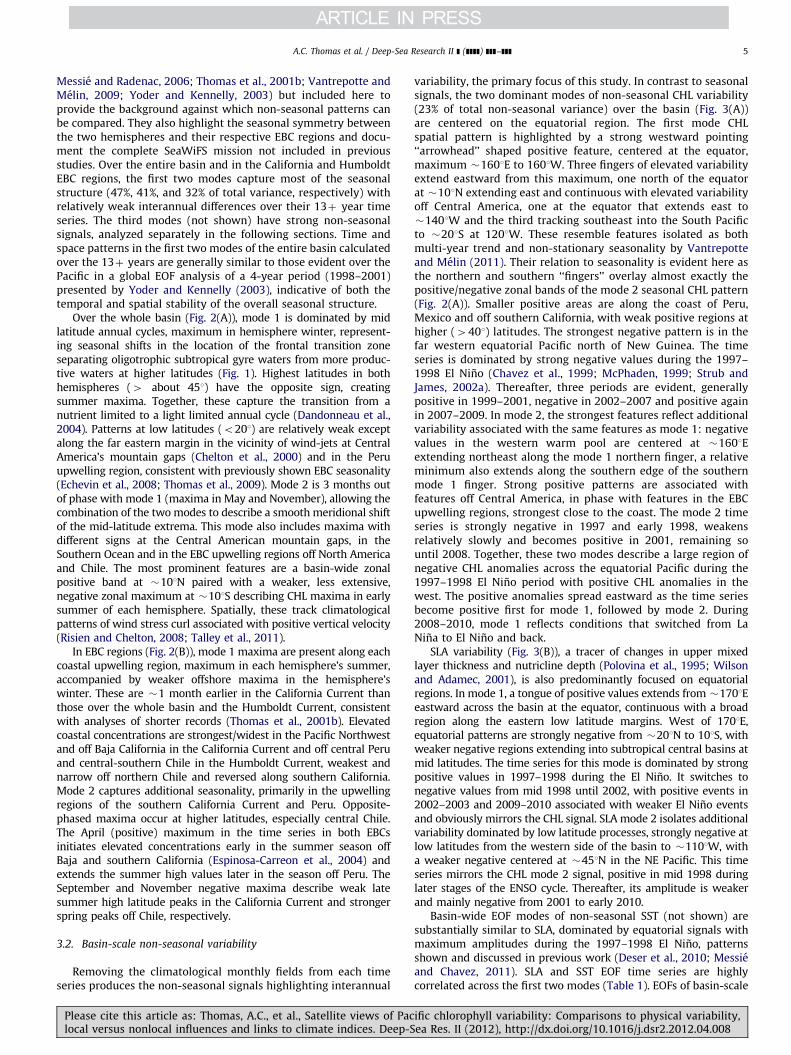
variability, the primary focus of this study. In contrast to seasonalsignals, the two dominant modes of non-seasonal CHL variability(23% of total non-seasonal variance) over the basin (Fig. 3(A))are centered on the equatorial region. The first mode CHLspatial pattern is highlighted by a strong westward pointing‘‘arrowhead’’ shaped positive feature, centered at the equator,maximum �1601E to 1601W. Three fingers of elevated variabilityextend eastward from this maximum, one north of the equatorat �101N extending east and continuous with elevated variabilityoff Central America, one at the equator that extends east to�1401W and the third tracking southeast into the South Pacificto �201S at 1201W. These resemble features isolated as bothmulti-year trend and non-stationary seasonality by Vantrepotteand Melin (2011). Their relation to seasonality is evident here asthe northern and southern ‘‘fingers’’ overlay almost exactly thepositive/negative zonal bands of the mode 2 seasonal CHL pattern(Fig. 2(A)). Smaller positive areas are along the coast of Peru,Mexico and off southern California, with weak positive regions athigher (4401) latitudes. The strongest negative pattern is in thefar western equatorial Pacific north of New Guinea. The timeseries is dominated by strong negative values during the 1997–1998 El Nino (Chavez et al., 1999; McPhaden, 1999; Strub andJames, 2002a). Thereafter, three periods are evident, generallypositive in 1999–2001, negative in 2002–2007 and positive againin 2007–2009. In mode 2, the strongest features reflect additionalvariability associated with the same features as mode 1: negativevalues in the western warm pool are centered at �1601Eextending northeast along the mode 1 northern finger, a relativeminimum also extends along the southern edge of the southernmode 1 finger. Strong positive patterns are associated withfeatures off Central America, in phase with features in the EBCupwelling regions, strongest close to the coast. The mode 2 timeseries is strongly negative in 1997 and early 1998, weakensrelatively slowly and becomes positive in 2001, remaining sountil 2008. Together, these two modes describe a large region ofnegative CHL anomalies across the equatorial Pacific during the1997–1998 El Nino period with positive CHL anomalies in thewest. The positive anomalies spread eastward as the time seriesbecome positive first for mode 1, followed by mode 2. During2008–2010, mode 1 reflects conditions that switched from LaNina to El Nino and back.

SLA variability (Fig. 3(B)), a tracer of changes in upper mixedlayer thickness and nutricline depth (Polovina et al., 1995; Wilsonand Adamec, 2001), is also predominantly focused on equatorialregions. In mode 1, a tongue of positive values extends from �1701Eeastward across the basin at the equator, continuous with a broadregion along the eastern low latitude margins. West of 1701E,equatorial patterns are strongly negative from �201N to 101S, withweaker negative regions extending into subtropical central basins atmid latitudes. The time series for this mode is dominated by strongpositive values in 1997–1998 during the El Nino. It switches tonegative values from mid 1998 until 2002, with positive events in2002–2003 and 2009–2010 associated with weaker El Nino eventsand obviously mirrors the CHL signal. SLA mode 2 isolates additionalvariability dominated by low latitude processes, strongly negative atlow latitudes from the western side of the basin to �1101W, witha weaker negative centered at �451N in the NE Pacific. This timeseries mirrors the CHL mode 2 signal, positive in mid 1998 duringlater stages of the ENSO cycle. Thereafter, its amplitude is weakerand mainly negative from 2001 to early 2010.

Basin-wide EOF modes of non-seasonal SST (not shown) aresubstantially similar to SLA, dominated by equatorial signals withmaximum amplitudes during the 1997–1998 El Nino, patternsshown and discussed in previous work (Deser et al., 2010; Messieand Chavez, 2011). SLA and SST EOF time series are highlycorrelated across the first two modes (Table 1). EOFs of basin-scale


dx.doi.org/10.1016/j.dsr2.2012.04.008

dx.doi.org/10.1016/j.dsr2.2012.04.008

dx.doi.org/10.1016/j.dsr2.2012.04.008

Fig. 3. The first two modes of an EOF decomposition over the whole basin of monthly non-seasonal (A) CHL concentrations and (B) SLA, showing their respective space

patterns, associated time series (CHL solid line, SLA dotted line) and the percent of total variance explained by each over the study period.

Table 1Correlations between whole-basin (Fig. 2) and equatorial EOF mode 1 and 2 time series of non-seasonal chlorophyll, SLA and SST signals (only those with significance

495% are shown). Bold values highlight whole basin—equatorial similarity.

Region Whole basin Equatorial

CHL SLA SST CHL SLA SST

M1 M2 M1 M2 M1 M2 M1 M2 M1 M2 M1 M2

Whole basinCHL

M1 1 – �0.95 – �0.93 – 0.99 – �0.93 – �0.90 –

M2 1 – �0.82 – �0.87 – 0.98 – �0.79 – �0.84

SLAM1 1 0.94 – �0.94 – 0.99 – 0.92 –

M2 1 0.81 – �0.79 – 0.97 – 0.74

SSTM1 1 �0.92 – 0.94 – 0.98 –

M2 1 �0.85 – 0.74 – 0.94

EquatorialCHL

M1 1 �0.92 – �0.90 –

M2 1 �0.77 – �0.85

SLAM1 1 0.94 –

M2 1 0.66

SSTM1 1 –

M2 1


Please cite this article as: Thomas, A.C., et al., Satellite views of Pacific chlorophyll variability: Comparisons to physical variability,local versus nonlocal influences and links to climate indices. Deep-Sea Res. II (2012), http://dx.doi.org/10.1016/j.dsr2.2012.04.008

dx.doi.org/10.1016/j.dsr2.2012.04.008

dx.doi.org/10.1016/j.dsr2.2012.04.008

dx.doi.org/10.1016/j.dsr2.2012.04.008


non-seasonal wind stress curl (not shown), however, are domi-nated by patterns over the Southern Ocean and neither their spacenor time patterns resemble those of CHL, SST or SLA.

Comparisons between the CHL patterns and those of SLA (andSST) in mode 1 (Fig. 3) show the canonical association of lower(higher) CHL values with elevated (decreased) SLA, indicative ofa thicker (thinner) mixed layer over the eastern basins and mainbasin gyres where signals are weaker (Wilson and Adamec, 2002).In equatorial regions where the signals are strong, CHL maximaappear most closely associated with the edges of SLA features,suggesting links to changes in the equatorial current structure(Wilson and Adamec, 2001). Space patterns in the two secondmodes are less similar and appear to capture different phases oftransition in the ENSO cycle (McPhaden, 1999), an observationsupported by slight differences in the timing of the 1998 maxima.The strong link between non-seasonal temporal CHL variabilityand satellite-measured physical variability evident in Fig. 3 isquantified in the correlations between modes 1 and 2 across CHL,SLA and SST (Table 1).

The extent of dominance of basin-scale non-seasonal modesby equatorial variability is investigated by calculating separateEOFs over a spatial domain restricted to 7201 of the equator (seeFig. 1). EOFs for CHL, SST and SLA in this equatorial corridor (notshown) have patterns that are essentially identical to thosefor the whole basin in the equatorial region of spatial overlap.Equatorial EOF time series are strongly correlated (all 40.94)with those of their basin-scale counterpart (Table 1) in bothmodes 1 and 2.

3.3. Extra-tropical patterns, symmetry and relationships to basin-

scale signals

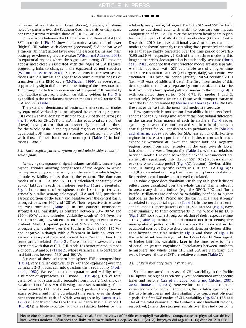
Removing the equatorial signal isolates variability occurring athigher latitudes allowing comparisons of the degree to whichhemispheres vary symmetrically and the extent to which higher-latitude variability tracks that at the equator. The dominantmodes of CHL, SLA and SST EOFs calculated separately over20–601 latitude in each hemisphere (see Fig. 1) are presented inFig. 4. In the northern hemisphere, mode 1 spatial patterns aregenerally similar among chlorophyll, SLA and SST, positive ineastern portions of the basin and negative over the central basin,strongest between 1601 and 1801W. Their respective time seriesare well correlated (Table 2). In the southern hemisphere,strongest CHL variability is centered between 801–1001W and1301–1601W at mid latitudes. Variability south of 401S (over theSouthern Ocean) is weak except for a small region west of NewZealand. Mode 1 spatial patterns of SLA and SST are similar,strongest and positive over the Southern Ocean (1001–1601W),and negative, although with differences in latitude, over theeastern subtropical gyre and around New Zealand. Their timeseries are correlated (Table 2). These modes, however, are notcorrelated with that of CHL. CHL mode 1 is better related to mode2 of both SLA and SST (Table 2), whose variance is also centered atmid latitudes between 1301 and 1601W.

For each of these southern hemisphere EOF decompositions(Fig. 4), very similar eigenvalues (% variance explained) over thedominant 2–3 modes call into question their separability (Northet al., 1982). We evaluate their separation and validity usinga number of approaches. CHL mode 1 (Fig. 4(A), 10% of totalvariance) is not statistically separate from mode 2 (not shown).Recalculation of this EOF following increased smoothing of theinitial monthly CHL fields (not shown) produced very similarspace patterns and highly correlated time series over the domi-nant three modes, each of which was separate by North et al.,1982) rule of thumb. We take this as evidence that CHL mode 1(Fig. 4(A)) is likely separate, but with statistics hidden by the


relatively noisy biological signal. For both SLA and SST we haveaccess to additional data with which to compare our modes.Computation of an SLA EOF over the southern hemisphere regionfor the full period of AVISO data availability (October 1992–December 2010, i.e., five additional years) produces dominantmodes (not shown) strongly resembling those presented and timeseries that are highly correlated over the time period of overlap(0.95 and 0.98, respectively). Each of the first three modes in thislonger time series decomposition is statistically separate (Northet al., 1982), evidence that our presented modes are also separate.A similar approach with SST data made use of a higher timeand space resolution data set (1/4 degree, daily) with which wecalculated EOFs over the period January 1982–December 2010(i.e., �16 years of additional data). The first three modes of thisdecomposition are clearly separate by North et al.’s criteria. Thefirst two modes have spatial patterns similar to those in Fig. 4(C)with correlated time series (0.76, 0.71, for modes 1 and 2,respectively). Patterns resemble those with strongest varianceover the Pacific presented by Messie and Chavez (2011). We takethese as evidence that the presented modes are separate.

How symmetric is non-seasonal variability in the two hemi-spheres? Spatially, taking into account the longitudinal differencein the eastern basin margin of each hemisphere, Fig. 4 showssymmetry between the northern and southern hemispheres inspatial pattern for SST, consistent with previous results (Shakunand Shaman, 2009) and also for SLA, less so for CHL. Positiveregions in the eastern portions of the basins mirror each other,expanding westward at lower and higher latitudes. Negativeregions trend from mid latitudes in the east towards lowerlatitudes in the west. Temporally (Table 2), while correlationsbetween modes 1 of each hemisphere of each measurement arestatistically significant, only that of SST (0.72) appears similarover the whole study period (Fig. 4(C), bottom). Obvious differ-ences in timing of specific events in CHL and SLA (Fig. 4(A)and (B)) are evident reducing their inter-hemisphere correlations.Respective second modes are not well correlated.

To what degree does dominant variability at higher latitudesreflect those calculated over the whole basin? This is relevantbecause many climate indices (e.g., the NPGO, PDO and NorthPacific Oscillation) are defined by variability confined to higherlatitudes in the North Pacific and the basin signals are stronglycorrelated to equatorial signals (Table 1). In the northern hemi-sphere, mode 1 space patterns of CHL, SLA and SST (Fig. 4) haveclear similarity to their counterparts in the whole basin EOFs(Fig. 3, SST not shown). Strong correlation of their respective timeseries (Table 2), indicate that dominant northern hemispherenon-equatorial patterns reflect those over the basin and in theequatorial corridor. Despite these correlations, an obvious differ-ence between the time series in Fig. 3 and those of Fig. 4 isthe reduced relative strength of the 1997–1998 El Nino signal.At higher latitudes, variability later in the time series is oftenof equal, or greater, magnitude. Correlations between southernhemisphere and whole basin CHL and SLA are significant butweak, however those of SST are relatively strong (Table 2).

3.4. Eastern boundary current variability

Satellite-measured non-seasonal CHL variability in the PacificEBC upwelling regions is relatively well documented over specifictimes and regions (Carr et al., 2002; Kahru and Mitchell, 2001,2002; Thomas et al., 2003). Here we focus on dominant coherentvariability over the entire EBC domains, their relative symmetry inthe two hemispheres and their similarity to concurrent physicalsignals. The first EOF modes of CHL variability (Fig. 5(A), 18% and16% of the total variance in the California and Humboldt regions,respectively) show the strongest signals over the study period in


dx.doi.org/10.1016/j.dsr2.2012.04.008

dx.doi.org/10.1016/j.dsr2.2012.04.008

dx.doi.org/10.1016/j.dsr2.2012.04.008

Fig. 4. The dominant modes of variability from EOF decompositions (calculated separately) over the North Pacific and the South Pacific study regions (201–601 latitude, see Fig. 1) for each of (A) CHL, (B) SLA and (C) SST (the first

two modes of SLA and SST in the southern hemisphere), showing those modes that have the most similar space pattern and most strongly correlated time series. Below each are their respective time series (bold line: northern

hemisphere, dotted line: southern hemisphere mode 1, thin solid line: southern hemisphere mode 2) and the % variance explained by each mode.

A.C

.T

ho

ma

set

al.

/D

eep-Sea

Resea

rchII]

(]]]])]]]–

]]]8

Ple

ase

citeth

isa

rticlea

s:T

ho

ma

s,A

.C.,

et

al.,

Sa

tellite

vie

ws

of

Pa

cific

chlo

rop

hy

llv

aria

bility

:C

om

pa

rison

sto

ph

ysica

lv

aria

bility

,lo

cal

ve

rsus

no

nlo

cal

infl

ue

nce

sa

nd

link

sto

clima

tein

dice

s.D

ee

p-S

ea

Re

s.II

(20

12

),h

ttp://d

x.d

oi.o

rg/1

0.1

01

6/j.d

sr2.2

01

2.0

4.0

08

dx.doi.org/10.1016/j.dsr2.2012.04.008

dx.doi.org/10.1016/j.dsr2.2012.04.008

dx.doi.org/10.1016/j.dsr2.2012.04.008

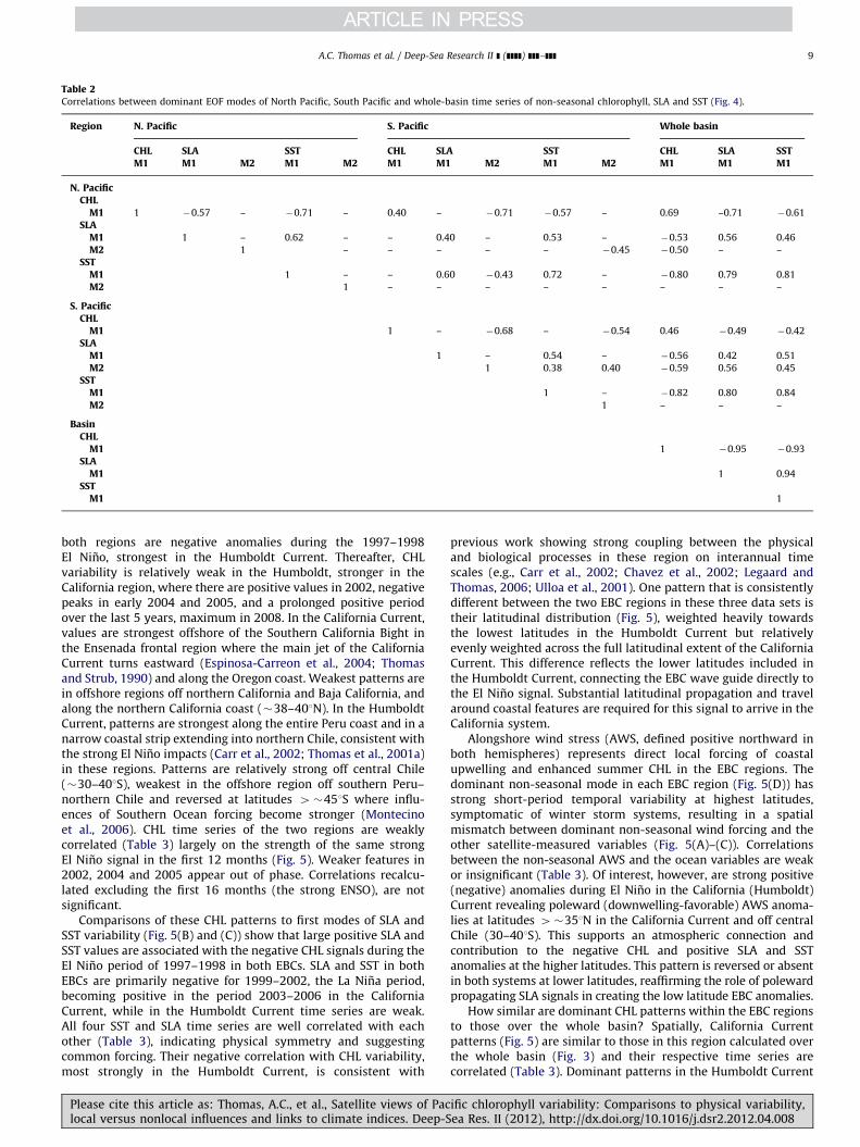
Table 2Correlations between dominant EOF modes of North Pacific, South Pacific and whole-basin time series of non-seasonal chlorophyll, SLA and SST (Fig. 4).

Region N. Pacific S. Pacific Whole basin

CHL SLA SST CHL SLA SST CHL SLA SSTM1 M1 M2 M1 M2 M1 M1 M2 M1 M2 M1 M1 M1

N. PacificCHL

M1 1 �0.57 – �0.71 – 0.40 – �0.71 �0.57 – 0.69 –0.71 �0.61

SLAM1 1 – 0.62 – – 0.40 – 0.53 – �0.53 0.56 0.46

M2 1 – – – – – �0.45 �0.50 – –

SSTM1 1 – – 0.60 �0.43 0.72 – �0.80 0.79 0.81

M2 1 – – – – – – – –

S. PacificCHL

M1 1 – �0.68 – �0.54 0.46 �0.49 �0.42

SLAM1 1 – 0.54 – �0.56 0.42 0.51

M2 1 0.38 0.40 �0.59 0.56 0.45

SSTM1 1 – �0.82 0.80 0.84

M2 1 – – –

BasinCHL

M1 1 �0.95 �0.93

SLAM1 1 0.94

SSTM1 1


both regions are negative anomalies during the 1997–1998El Nino, strongest in the Humboldt Current. Thereafter, CHLvariability is relatively weak in the Humboldt, stronger in theCalifornia region, where there are positive values in 2002, negativepeaks in early 2004 and 2005, and a prolonged positive periodover the last 5 years, maximum in 2008. In the California Current,values are strongest offshore of the Southern California Bight inthe Ensenada frontal region where the main jet of the CaliforniaCurrent turns eastward (Espinosa-Carreon et al., 2004; Thomasand Strub, 1990) and along the Oregon coast. Weakest patterns arein offshore regions off northern California and Baja California, andalong the northern California coast (�38–401N). In the HumboldtCurrent, patterns are strongest along the entire Peru coast and in anarrow coastal strip extending into northern Chile, consistent withthe strong El Nino impacts (Carr et al., 2002; Thomas et al., 2001a)in these regions. Patterns are relatively strong off central Chile(�30–401S), weakest in the offshore region off southern Peru–northern Chile and reversed at latitudes 4�451S where influ-ences of Southern Ocean forcing become stronger (Montecinoet al., 2006). CHL time series of the two regions are weaklycorrelated (Table 3) largely on the strength of the same strongEl Nino signal in the first 12 months (Fig. 5). Weaker features in2002, 2004 and 2005 appear out of phase. Correlations recalcu-lated excluding the first 16 months (the strong ENSO), are notsignificant.

Comparisons of these CHL patterns to first modes of SLA andSST variability (Fig. 5(B) and (C)) show that large positive SLA andSST values are associated with the negative CHL signals during theEl Nino period of 1997–1998 in both EBCs. SLA and SST in bothEBCs are primarily negative for 1999–2002, the La Nina period,becoming positive in the period 2003–2006 in the CaliforniaCurrent, while in the Humboldt Current time series are weak.All four SST and SLA time series are well correlated with eachother (Table 3), indicating physical symmetry and suggestingcommon forcing. Their negative correlation with CHL variability,most strongly in the Humboldt Current, is consistent with


previous work showing strong coupling between the physicaland biological processes in these region on interannual timescales (e.g., Carr et al., 2002; Chavez et al., 2002; Legaard andThomas, 2006; Ulloa et al., 2001). One pattern that is consistentlydifferent between the two EBC regions in these three data sets istheir latitudinal distribution (Fig. 5), weighted heavily towardsthe lowest latitudes in the Humboldt Current but relativelyevenly weighted across the full latitudinal extent of the CaliforniaCurrent. This difference reflects the lower latitudes included inthe Humboldt Current, connecting the EBC wave guide directly tothe El Nino signal. Substantial latitudinal propagation and travelaround coastal features are required for this signal to arrive in theCalifornia system.

Alongshore wind stress (AWS, defined positive northward inboth hemispheres) represents direct local forcing of coastalupwelling and enhanced summer CHL in the EBC regions. Thedominant non-seasonal mode in each EBC region (Fig. 5(D)) hasstrong short-period temporal variability at highest latitudes,symptomatic of winter storm systems, resulting in a spatialmismatch between dominant non-seasonal wind forcing and theother satellite-measured variables (Fig. 5(A)–(C)). Correlationsbetween the non-seasonal AWS and the ocean variables are weakor insignificant (Table 3). Of interest, however, are strong positive(negative) anomalies during El Nino in the California (Humboldt)Current revealing poleward (downwelling-favorable) AWS anoma-lies at latitudes 4�351N in the California Current and off centralChile (30–401S). This supports an atmospheric connection andcontribution to the negative CHL and positive SLA and SSTanomalies at the higher latitudes. This pattern is reversed or absentin both systems at lower latitudes, reaffirming the role of polewardpropagating SLA signals in creating the low latitude EBC anomalies.

How similar are dominant CHL patterns within the EBC regionsto those over the whole basin? Spatially, California Currentpatterns (Fig. 5) are similar to those in this region calculated overthe whole basin (Fig. 3) and their respective time series arecorrelated (Table 3). Dominant patterns in the Humboldt Current


dx.doi.org/10.1016/j.dsr2.2012.04.008

dx.doi.org/10.1016/j.dsr2.2012.04.008

dx.doi.org/10.1016/j.dsr2.2012.04.008

Fig. 5. The first modes of EOF decompositions of CHL, SLA, SST and alongshore wind stress over a 500 km wide region encompassing the main upwelling regions of the

California and Humboldt Current EBC regions, showing the space pattern of each and their respective time series (solid line: California, dotted line: Humboldt). The percent

variance each mode explains is given above the time series.



dx.doi.org/10.1016/j.dsr2.2012.04.008

dx.doi.org/10.1016/j.dsr2.2012.04.008

dx.doi.org/10.1016/j.dsr2.2012.04.008

Table 3Correlations between modes 1 of non-seasonal variability within each EBC region of chlorophyll, SLA, SST and alongshore wind stress (Fig. 5) and to whole basin mode 1

(Fig. 3).

Region California Current Humboldt Current Whole basin

CHL SLA SST s(as) CHL SLA SST s(as) CHL SLA SST

California CurrentCHL 1 �0.57 �0.67 – 0.43 �0.41 �0.57 – 0.46 �0.50 �0.41

SLA 1 0.87 �0.46 �0.55 0.77 0.62 – �0.84 0.85 0.84

SST 1 �0.38 �0.46 0.65 0.58 – �0.75 0.75 0.77

s(as) 1 – – – – – – –

Humboldt CurrentCHL 1 �0.72 �0.70 – 0.52 �0.54 �0.53

SLA 1 0.83 – �0.76 0.76 0.79

SST 1 – �0.62 0.59 0.64

s(as) 1 0.40 �0.43 �0.41

BasinCHL 1 �0.95 �0.93

SLA 1 0.94

SST 1

Fig. 6. Time series of three Pacific climate indices, the MEI, PDO and NPGO, over

the study period.


have spatial similarities to both modes of basin-wide CHL varia-bility (Fig. 3) and are temporally correlated with both (r¼0.52and 0.65, respectively), each stronger than those in the CaliforniaCurrent (emphasizing the Humboldt Current’s more direct equa-torial connection). Over the time window analyzed here, EBC CHLinterannual variability is strongly related to that over the wholebasin, contributing to the symmetry between systems and sug-gestive of common responses to climate signals of equatorialorigin.

3.5. Satellite-measured variability: Relationships to climate indices

The strongest non-seasonal signal over the 13-year study periodin most of the satellite-measured time series presented above is the1997–1998 El Nino, associated with positive anomalies of SLA andSST and negative anomalies in CHL. The MEI (Fig. 6), designedto track ENSO equatorial variability (Wolter and Timlin, 1998),is strongly correlated with the dominant mode of non-seasonalvariability of each satellite signal in each of the separate study areas(Table 4), most strongly (as expected) in the equatorial and wholebasin regions for SST and SLA. ENSO impacts on equatorial SST, SLAand CHL patterns are well documented (McClain et al., 2002;Murtugudde et al., 1999), as are satellite views of CHL in the twoEBC regions (Carr et al., 2002; Chavez et al., 2002; Kahru and Mitchell,2000; Thomas et al., 2001a). The MEI tracks the dominant mode ofmerged CHL-SST non-seasonal variability over the whole Pacific(Martinez et al., 2009) and explains �21% and 35% of mode 1 CHLvariability in the California and Humboldt systems, respectively, overthe complete SeaWiFS mission period. In the southern and northern


extra-tropics, the MEI accounts for 25% and 32%, respectively, of mode1 CHL variance (Table 4), similar to its impact on the EBCs. Thedifference is that the ENSO has a stronger effect on the northernhemisphere extra-tropical band than on its EBC, while its directconnection to South America delivers a greater impact on the south-ern hemisphere EBC.

The first EOF of SST north of 201N (Fig. 4) represents the purelysatellite-data analog of the PDO (Fig. 6) over the 13-year studyperiod. Not surprisingly, the space pattern looks indistinguishablefrom that of the PDO (see http://jisao.washington.edu/pdo/) andits time series is highly correlated (Table 4). The North PacificEOFs of SLA and CHL (Fig. 4) are similar to that of SST, their timeseries are highly correlated (Table 2), and each is more stronglyrelated to the PDO than the MEI (Table 4), the only region wherethis is true, reflecting their North Pacific emphasis. Chhak et al.(2009) discuss the linkage between SLA, SST and the PDO in theNorth Pacific. Satellite time series over both the whole basin andthe equatorial region are correlated with the PDO, consistent withprevious results (Martinez et al., 2009) and indicative of connec-tions between equatorial dynamics (ENSO) and North Pacificphysical variability discussed by many authors (Di Lorenzoet al., 2010; Newman et al., 2003; Strub and James, 2002c) butexpanded here to include a biological component. Restricted tovariability in the California Current, correlations to the PDO arestrong for SLA and SST, present but weaker for chlorophyll. Inthe southern hemisphere, the PDO is correlated to SST over theextra-tropics but not the EBC (Table 4), similar to the strongcorrelation between the dominant modes of SST in the northernand southern extra-tropics (Table 2 and Fig. 4). Do these satellitedata suggest a PDO-equivalent extra-tropical SST mode in thesouthern hemisphere? If so, does it resemble the PDO and is itconnected to ENSO? Figs. 4 and 6 and Tables 2 and 4 provideaffirmative answers. The dominant mode of satellite SST in thesouthern extra-tropics is similar (not identical) to its northerncounterpart; their correlation represents a common 52% of theirvariance. Both are correlated with the MEI and PDO (Table 4) andbasin-scale SST variability (Table 2), consistent with decadal-scaleSST linkages into both extra-tropical hemispheres from ENSOforcing (Shakun and Shaman, 2009).

Defined as the second mode of SLA variability in the northeastPacific, Di Lorenzo et al. (2008) suggest that the NPGO is theoceanic expression of the atmospheric forcing associated withthe North Pacific Oscillation that in turn is connected to ENSOvariability (Di Lorenzo et al., 2010). The NPGO represents lowfrequency gyre circulation variability with links to upwelling


http://jisao.washington.edu/pdo/

dx.doi.org/10.1016/j.dsr2.2012.04.008

dx.doi.org/10.1016/j.dsr2.2012.04.008

dx.doi.org/10.1016/j.dsr2.2012.04.008

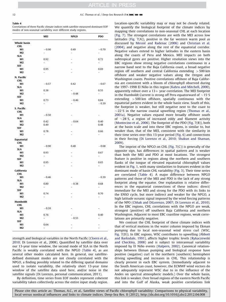
Table 4Correlations of three Pacific climate indices with satellite-measured dominant EOF

modes of non-seasonal variability over different study regions.

MEI NPGO PDO

Whole basinCHL

M1 �0.90 0.49 �0.70

M2 – – –

SLAM1 0.92 – 0.72

M2 – – –

SSTM1 0.95 – 0.69

M2 – – –

N. PacificCHL

M1 �0.57 0.42 �0.67

SLAM1 0.38 – 0.55

M2 – �0.48 –

SSTM1 0.73 �0.46 0.84

M2 – – �0.39

S. PacificCHL

M1 �0.50 – –

SLAM1 0.42 �0.64 0.40

M2 0.49 – 0.48

SSTM1 0.78 – 0.66

M2 – – –

EquatorialCHL

M1 �0.90 0.48 �0.68

SLAM1 0.93 – 0.67

M2 – – –

SSTM1 0.95 – 0.65

M2 – – –

CaliforniaCHL

M1 �0.46 – �0.39

SLAM1 0.80 �0.38 0.68

M2 – – –

SSTM1 0.74 – 0.70

M2 – – –

HumboldtCHL

M1 �0.59 – –

SLAM1 0.76 – 0.40

M2 – �0.55 –

SSTM1 0.64 – –

M2 – – –


strength and biological variables in the North Pacific (Cloern et al.,2010; Di Lorenzo et al., 2008). Quantified by satellite data overour 13-year time window, the second mode of SLA in the NorthPacific is weakly correlated with the NPGO (Table 4), as areseveral other modes calculated here. In general, our satellite-defined dominant modes are not closely correlated with theNPGO, a finding possibly related to the differing spatial domainsused to isolate variability, the relatively short 13-year timewindow of the satellite data used here, and/or noise in thesatellite signals (Di Lorenzo, personal communication, 2011).

By definition, time series from EOF modes represent coherentvariability taken collectively across the entire input study region.


Location-specific variability may or may not be closely related.We quantify the biological footprint of the climate indices bymapping their correlations to non-seasonal CHL at each location(Fig. 7). The strongest correlations are with the MEI across lowlatitudes (Fig. 7(A)), positive in the far western warm pool asdiscussed by Messie and Radenac (2006) and Christian et al.(2004), and negative along the rest of the equatorial corridor.Negative values extend to higher latitudes in the eastern basinalong the coasts of Peru and Mexico. MEI impacts on bothsubtropical gyres are positive. Higher resolution views into theEBC regions show strong negative correlations continuous in anarrow band next to the Baja California coast, a broad negativeregion off southern and central California extending 4500 kmoffshore and weaker negative values along the Oregon andWashington coasts. Positive correlations offshore of Baja Califor-nia are consistent with a bloom of chlorophyll observed duringthe 1997–1998 El Nino in this region (Kahru and Mitchell, 2000),apparently robust over a 13þ year correlation. The MEI footprintin the Humboldt Current is strong off Peru equatorward of �151Sextending 4500 km offshore, spatially continuous with theequatorial pattern evident in the whole basin view. South of this,the footprint is weaker, but still negative next to the coast to�221S in the narrow coastal upwelling region (Thomas et al.,2001a). Negative values expand more broadly offshore southof �281S, a region of increased eddy and filament activity(Montecino et al., 2006). The footprint of the PDO (Fig. 7(B)), bothat the basin scale and into these EBC regions, is similar to, butweaker than, that of the MEI, consistent with the similarity intheir time series over this 13-year period (Fig. 6) and connectionsin their forcing (Di Lorenzo et al., 2010; Shakun and Shaman,2009).

The imprint of the NPGO on CHL (Fig. 7(C)) is generally of theopposite sign, has differences in spatial pattern and is weakerthan both the MEI and PDO at most locations. The strongestfeature is positive in regions along the northern and southernflanks of the tongue of elevated equatorial chlorophyll valuesevident in Fig. 1, with many similarities to features evident in thedominant mode of basin CHL variability (Fig. 3). Their time seriesare correlated (Table 4). A major difference between NPGOpatterns and those of the MEI and PDO is the lack of any strongfootprint along the equator. One explanation is relative differ-ences in the equatorial connections of these indices: direct/immediate for the MEI and strong for the PDO with its links tothe ENSO cycle, but more indirect and weaker for the NPGO, ahigh latitude oceanic signal imposed by the wind forcing patternsof the NPO (Chhak and DiLorenzo, 2007; Di Lorenzo et al., 2010).In the EBC regions, CHL correlations with the NPGO are weak,strongest (positive) off southern Baja California and northernWashington. Adjacent to most EBC coastline regions, weak corre-lations are primarily negative.

We contrast the CHL footprint of these climate indices withthat of vertical motions in the water column imposed by Ekmanpumping due to local non-seasonal wind stress curl (WSC,Fig. 7(D)). In EBC regions, WSC contributes to upwelling (Abbottand Barksdale, 1991), affects higher trophic levels (Rykaczewskiand Checkley, 2008) and is subject to interannual variabilityimposed by El Nino events (Halpern, 2002). Canonical relation-ships between Ekman pumping and biological response havepositive (negative) curl in the northern (southern) hemispheredriving upwelling and increases in CHL. This relationship isclearly present in each EBC system. (Immediately adjacent tothe South American coast, however, the ECMWF wind vectors donot adequately represent WSC due to in the influence of theAndes on spectral atmospheric models.) Over the whole basin,this link is weaker. Over broad regions of the eastern North Pacificand into the Gulf of Alaska, weak positive correlations link


dx.doi.org/10.1016/j.dsr2.2012.04.008

dx.doi.org/10.1016/j.dsr2.2012.04.008

dx.doi.org/10.1016/j.dsr2.2012.04.008

Fig. 7. Projection correlations that map the footprint of the (A) MEI, (B) PDO, (C) NPGO and (D) non-seasonal local wind stress curl (WSC) variability onto non-seasonal CHL

at each grid location over the entire basin and in each EBC region. EBC values are the same as those over the basin but at higher spatial resolution and a different color scale

to improve coastal details. The MEI, PDO and NPGO are a single time series correlated to CHL at each CHL grid location. In (D), CHL was re-mapped to the coarser resolution

wind product grid and correlations of local wind stress curl with local CHL formed at each location.



dx.doi.org/10.1016/j.dsr2.2012.04.008

dx.doi.org/10.1016/j.dsr2.2012.04.008

dx.doi.org/10.1016/j.dsr2.2012.04.008

Fig. 8. Principal estimator patterns of CHL in the (A)–(C) California and (D)–(F) Humboldt EBC regions predicted by each of AWS (t), SLA and SST, showing the pairs of predictor and estimand (CHL) space patterns, their common

time series (solid line: California, dashed line: Humboldt), the percent of original predictor variance used by the PEP and the percent of the estimand (CHL) original total variance explained (‘‘skill’’ of the PEP).

A.C

.T

ho

ma

set

al.

/D

eep-Sea

Resea

rchII]

(]]]])]]]–

]]]1

4Ple

ase

citeth

isa

rticlea

s:T

ho

ma

s,A

.C.,

et

al.,

Sa

tellite

vie

ws

of

Pa

cific

chlo

rop

hy

llv

aria

bility

:C

om

pa

rison

sto

ph

ysica

lv

aria

bility

,lo

cal

ve

rsus

no

nlo

cal

infl

ue

nce

sa

nd

link

sto

clima

tein

dice

s.D

ee

p-S

ea

Re

s.II

(20

12

),h

ttp://d

x.d

oi.o

rg/1

0.1

01

6/j.d

sr2.2

01

2.0

4.0

08

dx.doi.org/10.1016/j.dsr2.2012.04.008

dx.doi.org/10.1016/j.dsr2.2012.04.008

dx.doi.org/10.1016/j.dsr2.2012.04.008


positive curl with increased CHL, but this is not true over thesubtropical gyre and is strongly reversed in the equatorialcorridor within 101 of the equator. This reversal at low latitudesis mirrored in the Southern Hemisphere where positive curl isassociated with increased CHL anomalies. The implications arethat in these low latitudes and the subtropical gyres, at the timeand space scales addressed here, interannual variability in localWSC plays a weaker role in modulating CHL than other processescaptured by the climate indices and satellite-measured SLA andSST and that these processes are associated with WSC signalsopposite to those that cause upwelling.

3.6. Physical–biological coupling: Within EBC regions

PEPs quantify local EBC time and space coupling betweendominant CHL modes of variability and physical modes, charac-terized here by AWS (t), SLA and SST. In the California Current(Fig. 8(A)–(C)), differences in the spatial patterns of forcing andCHL responses can be interpreted in comparison to previouslyviewed time/space patterns. The AWS space pattern is strongestand positive at higher latitudes, decreasing sharply at �351N,with weaker and reversed winds in the Southern California Bightand off Baja California, consistent with the geography of windstress (Bakun and Nelson, 1991) that shows maxima off northernCalifornia and weaker, but more persistent upwelling winds offBaja California. The SLA pattern is weighted higher towards thecoast and at lower latitudes, similar to SLA and SST in theHumboldt Current (Fig. 8(E) and (F)) and suggestive of coastallytrapped signals arriving from low latitudes. California Current SSThas no space pattern, implying a simple EBC-wide connectionbetween high SST and low CHL. Poleward AWS and positive SSTare coupled with similar negative CHL patterns; the main differ-ences are extensions of lower CHL right to the California coast,throughout the Southern California Bight and continuous alongBaja California coast in response to higher SST. CHL coupled tolocal SLA (Fig. 8(B)) is most similar to the CHL footprint of theMEI (Fig. 7), suggesting closer links to equatorial signals. EachCalifornia Current time series shows positive anomalies duringthe 1997–1998 El Nino period. Alongshore wind stress is positivenorthward, so association of positive times series with a positivewind spatial pattern indicates anomalously strong northward, orweaker equatorward (upwelling-favorable) winds during theEl Nino. Thereafter, a number of events are recognizable fromprevious studies. Enhanced CHL concentrations linked to colderSSTs are evident in late 2001 and 2002, associated with ananomalous advection of colder, nutrient-rich subarctic watersinto the northern California Current (Freeland et al., 2003;Thomas et al., 2003; Wheeler et al., 2003). In the first half of2005, all three time series switch abruptly from strongly positiveto weakly negative, the coupled response to delayed seasonalupwelling (Barth et al., 2007).

In the Humboldt Current (Fig. 8(D)–(F)), SLA and SST havesimilar spatial patterns strongly weighted to low latitudes. Each isdominated by positive 1997–1998 El Nino signals and each hasconsiderably more ‘‘skill’’ driving non-seasonal CHL than AWS.Both are linked to similar CHL patterns, with maximum negativeanomalies off Peru and coastal regions of northern Chile and againoff central Chile 30–401S. After the El Nino signal, the time seriesof both SLA and SST are weaker than those in the CaliforniaCurrent. This, and the increased skill of SLA and SST PEPs in theHumboldt Current are likely due to more direct linkages toequatorial signals and relatively weaker local processes thatinfluence non-seasonal CHL variability. The AWS pattern isdominated by variability at the highest latitudes where windsare dominated by Southern Ocean storms; non-seasonal AWSvariability over lower latitudes is comparatively weak. CHL


variability, however, is strongest off Peru (Fig. 5(A)) and thismismatch likely explains the lower ‘‘skill’’ of this PEP.

3.7. Physical–biological coupling: Equatorial links to regional

chlorophyll variability

EOFs and PEPs of variability at higher latitudes and in the EBCregions (Figs. 4, 5 and 8) are dominated by 1997–1998 El Ninosignals, well correlated to the MEI (Table 4) and clearly linked toequatorial variability. Here we contrast the views of ‘‘local’’coupling (Fig. 8) to those of non-local forcing of CHL by satel-lite-measured physical signals in the equatorial corridor. PEPsof equatorial SLA and SST generated substantially similar CHLpatterns and time series, as expected from the strong correlationof dominant equatorial SLA and SST EOF modes (Table 1). Forbrevity we show only those of SLA forcing CHL.

PEPs of equatorial SLA (and SST, not shown) forcing EBC CHLare shown in Fig. 9(A) and (B). Equatorially forced CaliforniaCurrent CHL PEP patterns are substantially similar to ‘‘local’’coupling (Fig. 8) south of �381N, but differ from those producedby local wind and SST (Fig. 8(A) and (C)) off Oregon and Washing-ton. This suggests patterns at these higher latitudes have strongerlinks to local (or non-equatorial) wind forcing and associated SSTresponse, consistent with links to NE Pacific atmospheric varia-bility in this region (Barth et al., 2007; Freeland et al., 2003; Struband James, 2002b). Their joint time series correlate with theMEI (0.75), but with a 1–2 month lag. In the Humboldt Current(Fig. 9(B)), equatorially forced CHL patterns are almost identical tothose forced locally (Fig. 8(E) and (F)), and their joint time seriescorrelation to the MEI is 0.75 with no lag, both consistent with amore direct connection to low latitude signals.

PEPs of equatorial SLA (and SST, not shown) forcing northernand southern hemisphere extra-tropical CHL variability (Fig. 9(C)and (D)) quantify coupling between equatorial signals (thesatellite-derived analogs to the MEI) and biology at extra-tropicallatitudes. These show biological patterns similar to those in Fig. 4:elevated equatorial SLA is associated with (a) increased CHLwithin the central gyres and (b) decreased CHL along the easternrim of the basin, strongest off south-central California, intothe Gulf of Alaska and off Chile. Equatorial SLA (and SST)patterns driving these CHL patterns, however, differ. NorthernHemisphere CHL is associated with forcing focused right along theequator, strongest in the central Pacific. The joint time series issynchronous with the MEI during 1997–1998 and lags it by �2months thereafter with an overall correlation of 0.81. SouthernHemisphere CHL is associated with equatorial SLA (and SST)patterns with a basin-wide zonal gradient, more similar to thoseevident in mode 2 of the basin-scale SLA EOF (Fig. 3) andsuggestive of later, transitional stages of the ENSO cycle. Thejoint PEP time series is weakly (but significantly) correlated withthe MEI (0.43) at a lag of 1 month. These differences point to moredirect coupling of North Pacific CHL to equatorial signals withmaximum coupling in each hemisphere linked to different phasesof the ENSO cycle.

3.8. Summary and conclusions

Both seasonal and non-seasonal biological and physical varia-bility in the Pacific measured by 13 years of concurrent satellitedata (CHL, SLA and SST) have strong symmetry about the equator-ial region. Seasonal patterns are strongest at mid latitudes andnon-seasonal patterns are focused along the equatorial corridor.

Dominant modes of non-seasonal EOFs calculated over thewhole basin and the equatorial (017201) region, are stronglycorrelated between regions and all variables, indicative of closebiological–physical coupling and equatorial domination of Pacific


dx.doi.org/10.1016/j.dsr2.2012.04.008

dx.doi.org/10.1016/j.dsr2.2012.04.008

dx.doi.org/10.1016/j.dsr2.2012.04.008

Fig. 9. Principal estimator patterns of CHL in the (A) California and (B) Humboldt EBC regions and the (C) North Pacific and (D) South Pacific, each predicted by equatorial

SLA, showing the pairs of predictor (SLA) and estimand (CHL) space patterns, the common time series (black) that modulate each, the percent of predictor (SLA) variance

used by the PEP and the percent of the estimand (CHL) variance explained (‘‘skill’’ of the PEP). Superimposed (blue) on each time series is the MEI (Fig. 6) as an aid for

comparison. (For interpretation of the references to color in this figure legend, the reader is referred to the web version of this article.)


variability. Wind EOFs are dominated by Southern Ocean varia-bility and poorly correlated with these signals.

Non-seasonal variability and biological–physical couplingfrom each of the study regions is strongly dominated by theENSO signals of 1997–1999, defined well by both basin-scale andequatorial SLA and SST EOF modes. Away from the equator, thisinteraction is strongest along the two Pacific EBC regions, extend-ing into the higher latitudes in the Humboldt Current and presentbut weaker into higher latitudes of California Current, wherevariability in years after the 1997–1999 ENSO signal is alsostrong. Dominant modes of SLA, SST and CHL in each study regionare most significantly correlated with the MEI, and less so with


the PDO except in the North Pacific. Links to the NPGO are weakin these data.

The spatial footprints of the MEI and PDO on non-seasonalchlorophyll patterns across the Pacific and in the EBC regions aresimilar, consistent with their coupled forcing, maximum along theequatorial corridor and also important in broad areas along thecoasts of both North and South America. The CHL footprint of non-seasonal wind stress curl is evident in the EBC regions but in otherregions, especially near the equator, the relationship is opposite tothat which would increase primary production, suggesting thatother non-seasonal forcing dominates in these regions. We realizethat these forcing mechanisms are not independent. Through the


dx.doi.org/10.1016/j.dsr2.2012.04.008

dx.doi.org/10.1016/j.dsr2.2012.04.008

dx.doi.org/10.1016/j.dsr2.2012.04.008


ENSO, the MEI is linked to the PDO and to the NPGO through theinfluence of atmospheric forcing on SST (and SLA) patterns athigher latitudes. Each also has connections to basin-scale windstress curl patterns and alongshore wind stress in the EBC regions.

Overall, the two EBCs show a gradation from control of CHL atlower latitudes by SLA to control by winds at higher latitudes. Inthe California Current, PEPs show coupling between CHL and localwind, SLA and SST, weakest for wind at low latitudes; time seriesof SLA and SST indicate equatorial forcing. In the HumboldtCurrent, PEPs show wind has less interaction with chlorophyllinterannual variability than SST and SLA, pointing to more directconnections of SLA and SST to equatorial signals. PEPs also showthe direct interaction of equatorial SLA and SST variability onEBC and higher latitude CHL, confirming the above links in EBCregions. The PEPs show that northern hemisphere extra-tropicalCHL lags equatorial signals by �2 months and is most closelylinked to El Nino anomalies in the central equatorial Pacific whilesouthern hemisphere extra-tropical CHL response is weaker, notlagged, and more closely linked to transitional equatorial patternsof the ENSO cycle.

Lastly, these time series are short by climate standards;requiring merging with additional ocean color missions toaddress decadal changes (Antoine et al., 2005; Martinez et al.,2009), and too short to address anthropogenic influences onoceanographic variability (Henson et al., 2010). They do, however,demonstrate the extent to which a single consistent mission(a) can quantify and reveal patterns of large-scale variabilityrelated to climate and (b) reflect variability tracked by majorclimate indices. They provide spatial details in CHL coupling toSLA and SST patterns unavailable from in situ data. Lags betweenthe MEI and PEP time series connecting equatorial SLA andCalifornia Current CHL spatial distributions highlight their poten-tial predictive capabilities and emphasizes the need to continuethese satellite observations into the future.

Acknowledgments

We thank the NASA SeaWiFS project team for providing theocean color satellite data, AVISO, NOAA/NWS/NCEP and NCAR foraccess to SLA, SST and wind data products, respectively, and thosepeople/organizations (referenced in the text) that make thevarious climate indices available. Funding for this work wasprovided by NSF as part of the U.S. GLOBEC program to ACT(OCE-0814413, OCE-0815051) and PTS (OCE-0815007). Addi-tional support for PTS was provided by the NASA Ocean SurfaceTopography Science Team (NNX08AR40G). Three anonymousreviewers provided constructive comments that resulted in alonger but more complete manuscript. This is contribution 718of the U.S. GLOBEC program.

References

Abbott, M.R., Barksdale, B., 1991. Phytoplankton pigment patterns and windforcing off central California. J. Geophys. Res. 96, 14649–14667.

Anderson, P.J., Paitt, J.F., 1999. Community reorganization in the Gulf of Alaskafollowing ocean climate regime shift. Mar. Ecol. Prog. Ser. 189, 117–123.

Antoine, D., Morel, A., Gordon, H.R., Banzon, V.F., Evans, E.H., 2005. Bridging oceancolor observations of the 1980s and 2000s in search of long-term trends.J. Geophys. Res., 110, http://dx.doi.org/10.1029/2004JC002620.

Bakun, A., Nelson, C.S., 1991. The seasonal cycle of wind-stress curl in subtropicaleastern boundary current regions. J. Phys. Oceanogr. 21, 1815–1834.

Barth, J.A., Menge, B.A., Lubchenco, J., Chan, F., Bane, J.A., Kirincich, A.R., McManus,M.A., Nielsen, K.J., Pierce, S.D., Washburn, L., 2007. Delayed upwelling altersnearshore coastal ocean ecosystems in the northern California current. Proc.Nat. Acad. Sci. 104, 3719–3724.

Bond, N.A., Harrison, D.E., 2000. The Pacific Decadal Oscillation, air–sea interactionand central north Pacific winter atmospheric regimes. Geophys. Res. Lett. 27,731–734.


Campbell, J.W., 1995. The lognormal distribution as a model for bio-opticalvariability in the sea. J. Geophys. Res. 100, 13,237–213,254.

Carr, M.E., Strub, P.T., Thomas, A.C., Blanco, J.L., 2002. Evolution of 1996–1999 La Ninaand El Nino conditions off the western coast of South America: a remote sensingperspective. J. Geophys. Res., 107, http://dx.doi.org/10.1029/2001JC001183.

Chavez, F.P., Messie, M., Pennington, J.T., 2011. Marine primary productionin relation to climate variability and change. Annu. Rev. Mar. Sci. 3,227–260, http://dx.doi.org/10.1146/annurev.marine.010908.163917.

Chavez, F.P., Pennington, J.T., Castro, C.G., Ryan, J.P., Michisaki, R.P., Schlining, B.,Walz, P., Buck, K.R., McFadyen, A., Collins, C.A., 2002. Biological and chemicalconsequences of the 1997–1998 El Nino in central California waters. Prog.Oceanogr. 54, 205–232.

Chavez, F.P., Strutton, P.G., Friederich, C.E., Feely, R.A., Feldman, G.C., Foley, D.C.,McPhaden, M.J., 1999. Biological and chemical response of the equatorialPacific Ocean to the 1997–98 El Nino. Science 286, 2126–2131.

Chelton, D.B., Freilich, M.H., Esbensen, S.K., 2000. Satellite observations of the windjets off the Pacific coast of central America. Part I: Case studies and statisticalcharacteristics. Monthly Weather Rev. 128, 1993–2018.

Chhak, K., DiLorenzo, E., 2007. Decadal variations in the California Current upwellingcells. Geophys. Res. Lett., 34, http://dx.doi.org/10.1029/2007GL030203.

Chhak, K.C., Di Lorenzo, E., Schneider, N., Cummins, P.F., 2009. Forcing of low-frequency ocean variability in the northeast Pacific. J. Clim. 22, 1255–1276.

Christian, J.R., Murtugudde, R., Ballabrera-Poy, J., McClain, C.R., 2004. A ribbon ofdark water: phytoplankton blooms in the meanders of the Pacific NorthEquatorial Countercurrent. Deep Sea Res. II 51, 209–228.

Cloern, J.E., Hieb, K.A., Jacobson, T., Sanso, B., Di Lorenzo, E., Stacey, M.T., Largier,J.L., Meiring, W., Peterson, W.T., Powell, T.M., Winder, M., Jassby, A.D., 2010.Biological communities in San Francisco Bay track large-scale climate forcingover the North Pacific. Geophys. Res. Lett., 37, http://dx.doi.org/10.1029/2010GL044774.

Dandonneau, Y., Deschamps, P.-Y., Nicolas, J.-M., Loisel, H., Blanchot, J., Montel, Y.,Thieuleux, F., Becu, G., 2004. Seasonal and interannual variability of oceancolor and composition of phytoplankton communities in the North Atlantic,equatorial Pacific and South Pacific. Deep Sea Res. II 51, 303–318.

Davis, R.E., 1977. Techniques for statistical analysis and prediction of geophysicalfluid systems. Geophys. Astrophys. Fluid Dyn. 8, 245–277.

Deser, C., Alexander, M.A., Xie, S.-P., Phillips, A.S., 2010. Sea surface temperaturevariability: patterns and mechanisms. Annu. Rev. Mar. Sci. 2, 115–143.

Di Lorenzo, E., Cobb, K.M., Furtado, J.C., Schneider, N., Anderson, B.T., Bracco, A.,Alexander, M.A., Vimont, D.J., 2010. Central Pacific El Nino and decadal climatechange in the North Pacific Ocean. Nat. Geosci. 3, http://dx.doi.org/10.1038/NGEO1984.

Di Lorenzo, E., Schneider, N., Cobb, K.M., Chhak, K., Franks, P.J.S., Miller, A.J.,McWilliams, J.C., Bograd, S.J., Arango, H., Curchister, E., Powell, T.M., Rivere, P.,2008. North Pacific Gyre Oscillation links ocean climate and ecosystemchange. Geophys. Res. Lett., 35, http://dx.doi.org/10.1029/2007GL032838.

Dommenget, D., Latif, M., 2002. A cautionary note on the interpretation of EOFs.J. Clim. 15, 216–225.

Echevin, V., Aumont, O., Ledesma, J., Flores, G., 2008. The seasonal cycle of surfacechlorophyll in the Peruvian upwelling system: a modelling study. Prog.Oceanogr. 79, 167–176.

Espinosa-Carreon, T.L., Strub, P.T., Beier, E., Ocampo-Torres, F., Gaxiola-Castro, G.,2004. Seasonal and interannual variability of satellite-derived chlorophyllpigment, surface height, and temperature off Baja California. J. Geophys. Res.109, http://dx.doi.org/10.1029/2003JC002105.

Freeland, H.J., Gatien, G., Huyer, A., Smith, R.L., 2003. Cold halocline in the northernCalifornia Current: an invasion of subarctic water. Geophys. Res. Lett. 30,http://dxdoi.org/10.1029/2002GL016663.

Halpern, D., 2002. Offshore Ekman transport and Ekman pumping off Peru duringthe 1997–1998 El Nino. Geophys. Res. Lett. 29, http://dx.doi.org/10.1029/2001GL014097.

Henson, S.A., Sarmiento, J.L., Dunne, J.P., Bopp, L., Doney, S.C., John, J., Beaulieu, C.,2010. Detection of anthropogentic climate change in satellite records of oceanchlorophyll and productivity. Biogeosciences 7, 621–640.

Hormazabal, S., Shaffer, G., Letelier, J., Ulloa, O., 2001. Local and remote forcing ofsea surface temperature in the coastal upwelling system off Chile. J. Geophys.Res. 106, 16657–16671.

Kahru, M., Mitchell, B.G., 2000. Influence of the 1997–98 El Nino on the surfacechlorophyll in the California Current. Geophys. Res. Lett. 27, 2937–2940.

Kahru, M., Mitchell, B.G., 2001. Seasonal and nonseasonal variability of satellite-derived chlorophyll and colored dissolved organic matter concentration in theCalifornia Current. J. Geophys. Res. 106, 2517–2529.

Kahru, M., Mitchell, B.G., 2002. Influence of the El Nino-La Nina cycle on satellite-derived primary production in the California Current. Geophys. Res. Lett. 29,http://dxdoi.org/10.1029/2002GL014963.

Large, W.G., Morzel, J., Crawford, G.B., 1995. Accounting for surface wave distor-tion of the marine wind profile in low-level ocean storms wind measurements.J. Phys. Oceanogr. 25, 2959–2971.

Legaard, K., Thomas, A.C., 2006. Spatial patterns in seasonal and interannualvariability of chlorophyll and surface temperature in the California Current.J. Geophys. Res., 111, http://dx.doi.org/10.1029/2005JC003282.

Lewis, M.R., Kuring, N., Yentsch, C., 1988. Global patterns of ocean transparency:implications for the new production of the open ocean. J. Geophys. Res. 93,6847–6856.

Longhurst, A., 1995. Seasonal cycles of pelagic production and consumption. Prog.Oceanogr. 36, 77–167.


dx.doi.org/10.1029/2004JC002620

dx.doi.org/10.1029/2004JC002620

dx.doi.org/10.1029/2004JC002620

dx.doi.org/10.1029/2001JC001183

dx.doi.org/10.1029/2001JC001183

dx.doi.org/10.1029/2001JC001183

dx.doi.org/10.1146/annurev.marine.010908.163917



dx.doi.org/10.1029/2007GL030203

dx.doi.org/10.1029/2007GL030203

dx.doi.org/10.1029/2007GL030203

dx.doi.org/10.1029/2010GL044774

dx.doi.org/10.1029/2010GL044774

dx.doi.org/10.1029/2010GL044774

dx.doi.org/10.1029/2010GL044774

dx.doi.org/10.1038/NGEO1984




dx.doi.org/10.1029/2007GL032838

dx.doi.org/10.1029/2007GL032838

dx.doi.org/10.1029/2007GL032838

dx.doi.org/10.1029/2003JC002105

dx.doi.org/10.1029/2003JC002105

dx.doi.org/10.1029/2003JC002105

dx.doi.org/10.1029/2002GL016663

dx.doi.org/10.1029/2002GL016663

dx.doi.org/10.1029/2002GL016663

dx.doi.org/10.1029/2001GL014097

dx.doi.org/10.1029/2001GL014097

dx.doi.org/10.1029/2001GL014097

dx.doi.org/10.1029/2001GL014097

dx.doi.org/10.1029/2002GL014963

dx.doi.org/10.1029/2002GL014963

dx.doi.org/10.1029/2002GL014963

dx.doi.org/10.1029/2005JC003282

dx.doi.org/10.1029/2005JC003282

dx.doi.org/10.1029/2005JC003282

dx.doi.org/10.1016/j.dsr2.2012.04.008

dx.doi.org/10.1016/j.dsr2.2012.04.008

dx.doi.org/10.1016/j.dsr2.2012.04.008


Mantua, N.J., Hare, S.R., 2002. The Pacific Decadal Oscillation. J. Oceanogr. 58,35–44.

Martinez, E., Antoine, D., D’Ortenzio, F., Gentili, B., 2009. Climate-drivenbasin-scale decadal oscillations of oceanic phytoplankton. Science 326,1253–1256.

McClain, C.R., Christian, J.R., Signorini, S.R., Lewis, M.R., Asanuma, I., Turk, D.,Dupouy-Douchement, C., 2002. Satellite ocean-color observations of thetropical Pacific Ocean. Deep Sea Res. Part II 49, 2533–2560.

McPhaden, M.J., 1999. Genesis and evolution of the 1997–98 El Nino. Science 283,950–954.

Messie, M., Chavez, F., 2011. Global modes of sea surface temperature variability inrelation to regional climate indices. J. Clim. 24, 4314–4331.

Messie, M., Radenac, M.-H., 2006. Seasonal variability of the surface chlorophyll inthe western tropical Pacific from SeaWiFS data. Deep Sea Res. 53, 1581–1600.

Miller, A.J., Chai, F., Chiba, S., Moisan, J.R., Neilson, D.J., 2004. Decadal-scale climateand ecosystem interactions in the North Pacific Ocean. J. Oceanogr. 60,163–188.

Montecino, V., Strub, P.T., Chavez, F.P., Thomas, A., Tarazona, J., Baumgartner, T.,2006. Bio–physical interactions off western South America. In: Robinson, A.R.,Brink, K.H. (Eds.), The Global Coastal Ocean Interdisciplinary Regional Studiesand Syntheses. Harvard university Press, Cambridge, pp. 329–390.

Murtugudde, R.G., Signorini, S.R., Christian, J.R., Busalacchi, A.J., McClain, C.R.,Picaut, J., 1999. Ocean color varability of the tropical Indo-Pacific basin observedby SeaWiFS during 1997–1998. J. Geophys. Res. 104, 18,351–18,366.

Newman, M., Compo, G.P., Alexander, M.A., 2003. ENSO-forced variability of thePacific Decadal Oscillation. J. Clim. 16, 3853–3857.

North, G.R., Bell, T.L., Cahalan, R.F., Moeng, F.J., 1982. Sampling errors in theestimation of empirical orthogonal functions. Monthly Weather Rev. 110,699–706.

O’Reilly, J.E., Maritorena, S., Mitchell, B.G., Siegel, D.A., Carder, K.L., Garver, S.A.,Kahru, M., McClain, C., 1998. Ocean color chlorophyll algorithms for SeaWiFS.J. Geophys. Res. 103, 24937–24953.

Overland, J.E., Preisendorfer, R.W., 1982. A significance test for principal compo-nents applied to a cyclone climatology. Monthly Weather Rev. 110, 1–4.

Philander, S.G., 1999. A review of tropical ocean–atmosphere interactions. Tellus51, 71–90.

Polovina, J.J., Mitchum, G.T., Evans, G.T., 1995. Decadal and basin-scale variation inmixed layer depth and the impact on biological production in the central andNorth Pacific, 1960–88. Deep Sea Res. 42, 1701–1716.

Reynolds, R.W., Rayner, N.A., Smith, T.M., Stokes, D.C., Wang, W., 2002. Animproved in situ and satellite SST analysis for climate. J. Clim. 15, 1609–1625.

Risien, C.M., Chelton, D.B., 2008. A global climatology of surface wind and windstress curl fields from eight years of QuikSCAT scatterometer data. J. Phys.Oceanogr. 38, 2379–2413.

Rykaczewski, R.R., Checkley, D.M., 2008. Influence of ocean winds on the pelagicecosystem in upwelling regions. Proc. Nat. Acad. Sci. U.S.A. 105, 1965–1970.

Schwing, F.B., Mendelssohn, R., Bograd, S.J., Overland, J.E., Wang, M., Ito, S., 2010.Climate change, teleconnection patterns, and regional processes forcingmarine populations in the Pacific. J. Mar. Syst. 79, 245–257.

Shakun, J.D., Shaman, J., 2009. Tropical origins of North and South Pacific decadalvariability. Geophys. Res. Lett. 36, http://dx.doi.org/10.1029/2009gl040313.

Signorini, S.R., McClain, C.R., 2012. Subtropical gyre variability as seen fromsatellites. Remote Sens. Lett. 3, 471–479.


Strub, P.T., James, C., 2002a. The 1997–1998 oceanic El Nino signal along thesoutheast and northeast Pacific boundaries—an altimetric view. Prog. Oceanogr.54, 439–458.

Strub, P.T., James, C., 2002b. Altimeter-derived surface circulation in the large-scale NE Pacific Gyres. Part 1. Seasonal variability. Prog. Oceanogr. 53,163–183.

Strub, P.T., James, C., 2002c. Altimeter-derived surface circulation in the large-scale NE Pacific Gyres. Part 2: 1997–1998 El Nino anomalies. Prog. Oceanogr.53, 185–214.

Strub, P.T., James, C., Thomas, A.C., Abbott, M.R., 1990. Seasonal and nonseasonalvariability of satellite-derived surface pigment concentration in the CaliforniaCurrent. J. Geophys. Res. 95, 11501–11530.

Talley, L.D., Pickard, G.L., Emery, W.J., Swift, J.H., 2011. Descriptive PhysicalOceanography: An Introduction, 6th ed. Elsevier, London.

Thomas, A.C., Blanco, J.L., Carr, M.E., Strub, P.T., Osses, J., 2001a. Satellite-measuredchlorophyll and temperature variability off northern Chile during the 1996–1998La Nina and El Nino. J. Geophys. Res. 106, 899–915.

Thomas, A.C., Brickley, P., Weatherbee, R., 2009. Interannual variability in chlor-ophyll concentrations in the Humboldt and California current systems. Prog.Oceanogr. 83, 386–392.

Thomas, A.C., Carr, M.E., Strub, P.T., 2001b. Chlorophyll variability in easternboundary currents. Geophys. Res. Lett. 28, 3421–3424.

Thomas, A.C., Strub, P.T., 1990. Seasonal and interannual variability of pigmentconcentrations across a California current frontal zone. J. Geophys. Res. 95,13023–13042.

Thomas, A.C., Strub, P.T., Brickley, P., 2003. Anomalous satellite-measured chlor-ophyll concentrations in the northern California Current in 2001–2002.Geophys. Res. Lett. 30, http://dx.doi.org/10.1029/2003GL017409.

Ulloa, O., Escribano, N., Hormazabal, S., Quinones, R.A., Gonzalez, R.R., Ramos, M.,2001. Evolution and biological effects of the 1997–98 El Nino in the upwellingecosystem off northern Chile. Geophys. Res. Lett. 28, 1591–1594.

Vantrepotte, V., Melin, F., 2009. Temporal variability of 10-year global SeaWiFStime-series of phytoplankton chlorophyll a concentration. ICES J. Mar. Sci. 66,1547–1556.

Vantrepotte, V., Melin, F., 2011. Inter-annual variations in the SeaWiFS globalchlorophyll a concentration (1997–2007). Deep Sea Res. Part I 58, 429–441.

Wheeler, P.A., Huyer, A., Fleischbein, J., 2003. Cold halocline, increased nutrients andhigher chlorophyll off Oregon in 2002. Geophys. Res. Lett. 30, http://dx.doi.org/10.1029/2003GL017395.

Wilson, C., Adamec, D., 2001. Correlations between surface chlorophyll and seasurface height in the tropical Pacific during the 1997–1999 El Nino-SouthernOscillation event. J. Geophys. Res. Oceans 106, 31175–31188.

Wilson, C., Adamec, D., 2002. A global view of bio-physical coupling from SeaWiFSand TOPEX satellite data, 1997–2001. Geophys. Res. Lett. 29, http://dx.doi.org/10.1029/2003GL017770.

Wolter, K., Timlin, M.S., 1998. Measuring the strength of ENSO events: how does1997–98 rank. Weather 53, 315–324.

Yoder, J.A., Kennelly, M.A., 2003. Seasonal and ENSO variability in global oceanphytoplankton chlorophyll derived from 4 years of SeaWiFS measurements.Global Biogeochem. Cycles, 17, http://dx.doi.org/10.1029/2002gb001942.

Yoder, J.A., Kennelly, M.A., Doney, S.C., Lima, I.D., 2010. Are trends in SeaWiFSchlorophyll time-series unusual relative to historic variability. Acta Oceanolog.Sin. 29, 1–4.


dx.doi.org/10.1029/2009gl040313

dx.doi.org/10.1029/2009gl040313

dx.doi.org/10.1029/2009gl040313

dx.doi.org/10.1029/2003GL017409

dx.doi.org/10.1029/2003GL017409

dx.doi.org/10.1029/2003GL017409

dx.doi.org/10.1029/2003GL017395

dx.doi.org/10.1029/2003GL017395

dx.doi.org/10.1029/2003GL017395

dx.doi.org/10.1029/2003GL017395

dx.doi.org/10.1029/2003GL017770

dx.doi.org/10.1029/2003GL017770

dx.doi.org/10.1029/2003GL017770

dx.doi.org/10.1029/2003GL017770

dx.doi.org/10.1029/2002gb001942

dx.doi.org/10.1029/2002gb001942

dx.doi.org/10.1029/2002gb001942

dx.doi.org/10.1016/j.dsr2.2012.04.008

dx.doi.org/10.1016/j.dsr2.2012.04.008

dx.doi.org/10.1016/j.dsr2.2012.04.008

deep-sea research ii€¦ · surface chlorophyll as the primary variable of interest; (2) con-...

Documents