1

Deep Multi-task Learningfor Railway Track Inspection

Xavier Gibert, Student Member, IEEE, Vishal M. Patel, Member, IEEE, and Rama Chellappa, Fellow, IEEE

Abstract—Railroad tracks need to be periodically inspectedand monitored to ensure safe transportation. Automated trackinspection using computer vision and pattern recognition meth-ods have recently shown the potential to improve safety byallowing for more frequent inspections while reducing humanerrors. Achieving full automation is still very challenging dueto the number of different possible failure modes as well as thebroad range of image variations that can potentially trigger falsealarms. Also, the number of defective components is very small,so not many training examples are available for the machine tolearn a robust anomaly detector. In this paper, we show thatdetection performance can be improved by combining multipledetectors within a multi-task learning framework. We show thatthis approach results in better accuracy in detecting defects onrailway ties and fasteners.

Index Terms—Railway track inspection, Multi-task Learning,Deep Convolutional Neural Networks, Material Identification.

I. INTRODUCTION

MONITORING the condition of railway components isessential to ensure train safety, especially on High

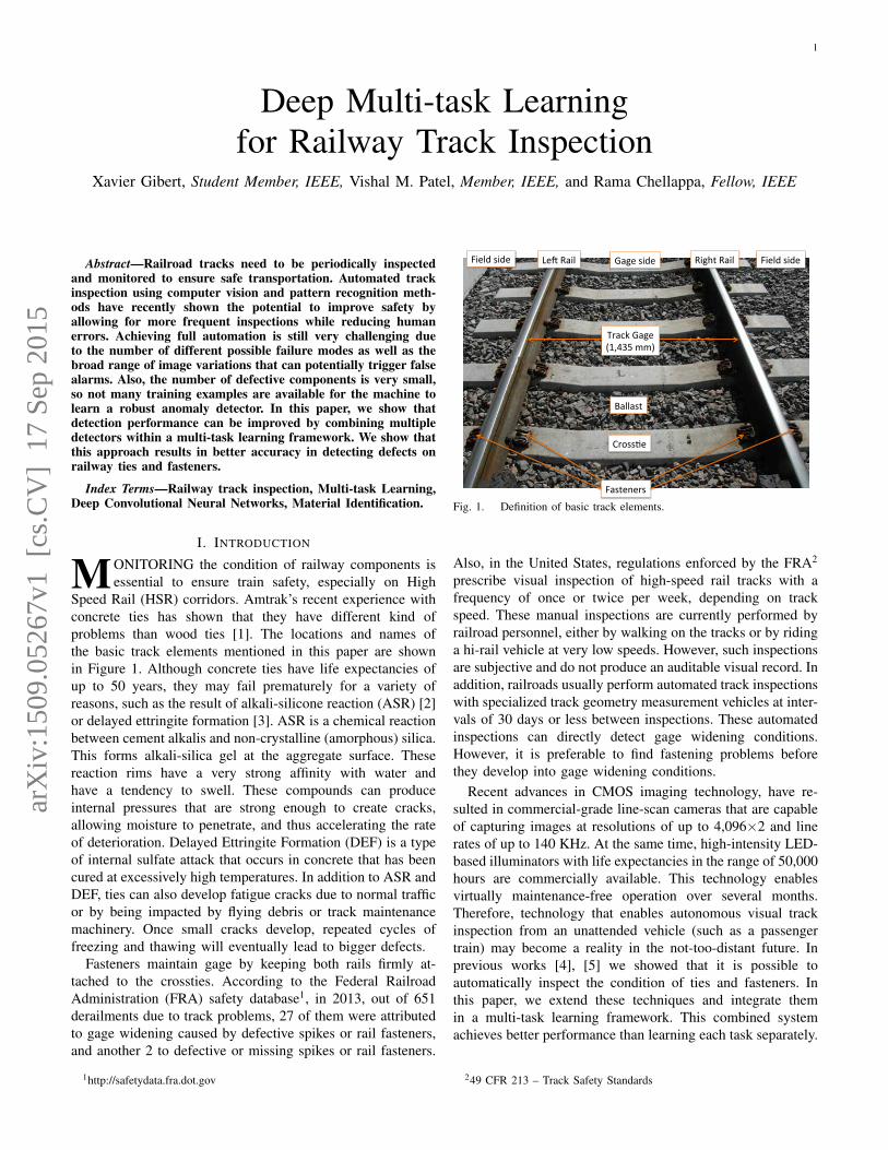
Speed Rail (HSR) corridors. Amtrak’s recent experience withconcrete ties has shown that they have different kind ofproblems than wood ties [1]. The locations and names ofthe basic track elements mentioned in this paper are shownin Figure 1. Although concrete ties have life expectancies ofup to 50 years, they may fail prematurely for a variety ofreasons, such as the result of alkali-silicone reaction (ASR) [2]or delayed ettringite formation [3]. ASR is a chemical reactionbetween cement alkalis and non-crystalline (amorphous) silica.This forms alkali-silica gel at the aggregate surface. Thesereaction rims have a very strong affinity with water andhave a tendency to swell. These compounds can produceinternal pressures that are strong enough to create cracks,allowing moisture to penetrate, and thus accelerating the rateof deterioration. Delayed Ettringite Formation (DEF) is a typeof internal sulfate attack that occurs in concrete that has beencured at excessively high temperatures. In addition to ASR andDEF, ties can also develop fatigue cracks due to normal trafficor by being impacted by flying debris or track maintenancemachinery. Once small cracks develop, repeated cycles offreezing and thawing will eventually lead to bigger defects.

Fasteners maintain gage by keeping both rails firmly at-tached to the crossties. According to the Federal RailroadAdministration (FRA) safety database1, in 2013, out of 651derailments due to track problems, 27 of them were attributedto gage widening caused by defective spikes or rail fasteners,and another 2 to defective or missing spikes or rail fasteners.

1http://safetydata.fra.dot.gov

Le#  Rail   Right  Rail  

Ballast  

Fasteners  

Cross3e  

Field  side   Field  side  Gage  side  

Track  Gage  (1,435  mm)  

Fig. 1. Definition of basic track elements.

Also, in the United States, regulations enforced by the FRA2

prescribe visual inspection of high-speed rail tracks with afrequency of once or twice per week, depending on trackspeed. These manual inspections are currently performed byrailroad personnel, either by walking on the tracks or by ridinga hi-rail vehicle at very low speeds. However, such inspectionsare subjective and do not produce an auditable visual record. Inaddition, railroads usually perform automated track inspectionswith specialized track geometry measurement vehicles at inter-vals of 30 days or less between inspections. These automatedinspections can directly detect gage widening conditions.However, it is preferable to find fastening problems beforethey develop into gage widening conditions.

Recent advances in CMOS imaging technology, have re-sulted in commercial-grade line-scan cameras that are capableof capturing images at resolutions of up to 4,096×2 and linerates of up to 140 KHz. At the same time, high-intensity LED-based illuminators with life expectancies in the range of 50,000hours are commercially available. This technology enablesvirtually maintenance-free operation over several months.Therefore, technology that enables autonomous visual trackinspection from an unattended vehicle (such as a passengertrain) may become a reality in the not-too-distant future. Inprevious works [4], [5] we showed that it is possible toautomatically inspect the condition of ties and fasteners. Inthis paper, we extend these techniques and integrate themin a multi-task learning framework. This combined systemachieves better performance than learning each task separately.

249 CFR 213 – Track Safety Standards

arX

iv:1

509.

0526

7v1

[cs

.CV

] 1

7 Se

p 20

15

2

A. Organization of the paper

This paper is organized as follows. Related works on inspec-tion of railway tracks using computer vision are discussed insection II. The problem addressed in this paper is described insection III. Overall approach and system architecture is pre-sented in section IV. Material classification, segmentation andtie assessment algorithm is described in section V. Fastenerdetection and assessment algorithm is described in section VI.Experimental results are presented in section VII, and sectionVIII concludes the paper with a brief summary and discussion.

II. RELATED WORKS

A. Railway Track Inspection

Since the pioneering work by Trosino et al. [6], [7], ma-chine vision technology has been gradually adopted by therailway industry as a track inspection technology. Those firstgeneration systems were capable of collecting images of therailway right of way and storing them for later review, but theydid not facilitate any automated detection. As faster processinghardware became available, several vendors began to introducevision systems with increasing automation capabilities.

In [8], [9], Marino et al. describe their VISyR system,which detects hexagonal-headed bolts using two 3-layer neuralnetworks (NN) running in parallel. Both networks take the 2-level discrete wavelet transform (DWT) of a 24×100 pixelsliding window (their images use non-square pixels) as aninput to generate a binary output indicating the presence ofa fastener. The difference is that the first NN uses Daubechieswavelets, while the second one uses Haar wavelets. Thiswavelet decomposition is equivalent to performing edge detec-tion at different scales with two different filters. Both neuralnetworks are trained with same examples. The final decisionis made using the maximum output of each neural network.

In [10], [11], Gibert et al. describe their VisiRail systemfor joint bar inspection. The system is capable of collectingimages on each rail side, and finding cracks on joint barsusing edge detection and a Support Vector Machine (SVM)classifier that analyzes features extracted from these edges. In[12], Babenko describes a fastener detection method basedon a convolutional filter bank that is applied directly tointensity images. Each type of fastener has a single filterassociated with it, whose coefficients are calculated usingan illumination-normalized version of the Optimal TradeoffMaximum Average Correlation Height (OT-MACH) filter [13].This approach allowed accurate fastener detection and local-ization and achieved over 90% fastener detection rate on adataset of 2,436 images. However, the detector was not testedon longer sections of track. In [14], Resendiz et al. use textureclassification via a bank of Gabor filters followed by an SVMto determine the location of rail components such as crosstiesand turnouts. They also use the MUSIC algorithm to findspectral signatures to determine expected component locations.In [15], Li et al. describe a system for detecting tie platesand spikes. Their method, which is described in more detailin [16], uses an AdaBoost-based object detector [17] with amodel selection mechanism that assigns the object class thatproduces the highest number of detections within a window

of 50 frames. Table I summarizes several systems reported inthe literature.

B. Convolutional Neural Networks

The idea of enforcing translation invariance in neural net-works via weight sharing goes back to Fukoshima’s Neocog-nitron [27]. Based on this idea, LeCun et al. developed theconcept into Deep Convolutional Neural Networks (DCNN)and used it for digit recognition [28], and later for moregeneral optical character recognition (OCR) [29]. During thelast few years, DCNNs have become ubiquitous in achievingstate-of-the-art results in image classification [30], [31] andobject detection [32]. This resurgence of DCNNs has beenfacilitated by the availability of efficient GPU implementationsand open source libraries such as Caffe [33] and Torch7 [34].More recently, DCNNs have been used for semantic imagesegmentation. For example, the work of [35] shows how aDCNN can be converted to a Fully Convolutional Network(FCN) by replacing fully-connected layers with convolutionalones.

C. Multi-task Learning

Multi-task learning (MTL) is an inductive transfer learningtechnique in which two or more learning machines are trainedcooperatively [36]. It is a generalization of multi-label learningin which each training sample has only been labeled forone of the tasks. In MTL settings there is a mechanismin which knowledge learned for one task is transferred tothe other tasks [37]. The idea is that each task can benefitby reusing knowledge that has been learned while trainingfor the other tasks. Backpropagation has been recognized asan effective method for learning distributed representations[38]. For instance, in multitask neural networks, we jointlyminimize one global loss function

Φ =

T∑t=1

λt

Nt∑i=1

Et (f(xti), yti) , (1)

where T is the number of tasks, Nt is the number of trainingsamples for task t, yti is the ground truth label for trainingsample xti, f is the the multi-output function computed by thenetwork, and Et is the loss function for task t. This contrastswith the Single Task Learning (STL) setting, in which weminimize T independent loss functions

Φt =

Nt∑i=1

Et (ft(xti), yti) , t ∈ {1 . . . T}. (2)

In MTL, the weighting factor λt is necessary to compensatefor imbalances in the complexity of the different tasks andthe amount of training data available. When using back-propagation, it is necessary to adjust λt’s to ensure that alltasks are learning at optimal rates.

D. One-shot Learning

To achieve good generalization performance, traditionalmachine learning methods require a minimum number of

3

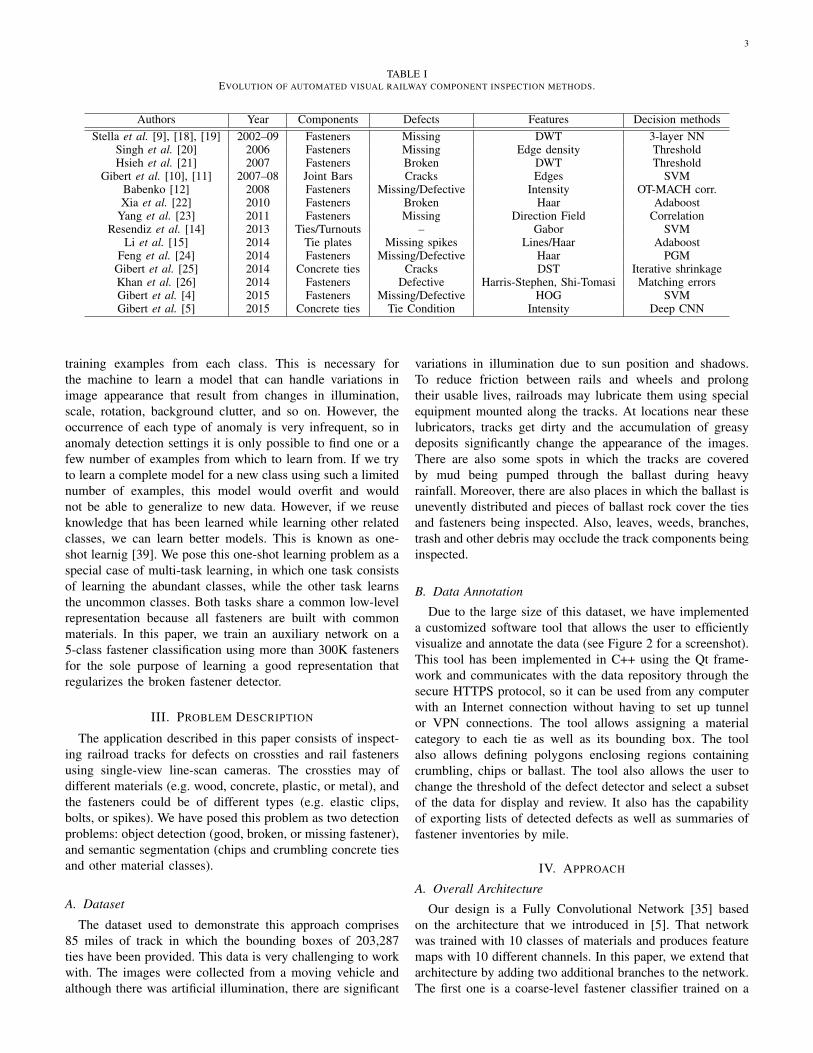
TABLE IEVOLUTION OF AUTOMATED VISUAL RAILWAY COMPONENT INSPECTION METHODS.

Authors Year Components Defects Features Decision methodsStella et al. [9], [18], [19] 2002–09 Fasteners Missing DWT 3-layer NN

Singh et al. [20] 2006 Fasteners Missing Edge density ThresholdHsieh et al. [21] 2007 Fasteners Broken DWT Threshold

Gibert et al. [10], [11] 2007–08 Joint Bars Cracks Edges SVMBabenko [12] 2008 Fasteners Missing/Defective Intensity OT-MACH corr.Xia et al. [22] 2010 Fasteners Broken Haar Adaboost

Yang et al. [23] 2011 Fasteners Missing Direction Field CorrelationResendiz et al. [14] 2013 Ties/Turnouts – Gabor SVM

Li et al. [15] 2014 Tie plates Missing spikes Lines/Haar AdaboostFeng et al. [24] 2014 Fasteners Missing/Defective Haar PGM

Gibert et al. [25] 2014 Concrete ties Cracks DST Iterative shrinkageKhan et al. [26] 2014 Fasteners Defective Harris-Stephen, Shi-Tomasi Matching errorsGibert et al. [4] 2015 Fasteners Missing/Defective HOG SVMGibert et al. [5] 2015 Concrete ties Tie Condition Intensity Deep CNN

training examples from each class. This is necessary forthe machine to learn a model that can handle variations inimage appearance that result from changes in illumination,scale, rotation, background clutter, and so on. However, theoccurrence of each type of anomaly is very infrequent, so inanomaly detection settings it is only possible to find one or afew number of examples from which to learn from. If we tryto learn a complete model for a new class using such a limitednumber of examples, this model would overfit and wouldnot be able to generalize to new data. However, if we reuseknowledge that has been learned while learning other relatedclasses, we can learn better models. This is known as one-shot learnig [39]. We pose this one-shot learning problem as aspecial case of multi-task learning, in which one task consistsof learning the abundant classes, while the other task learnsthe uncommon classes. Both tasks share a common low-levelrepresentation because all fasteners are built with commonmaterials. In this paper, we train an auxiliary network on a5-class fastener classification using more than 300K fastenersfor the sole purpose of learning a good representation thatregularizes the broken fastener detector.

III. PROBLEM DESCRIPTION

The application described in this paper consists of inspect-ing railroad tracks for defects on crossties and rail fastenersusing single-view line-scan cameras. The crossties may ofdifferent materials (e.g. wood, concrete, plastic, or metal), andthe fasteners could be of different types (e.g. elastic clips,bolts, or spikes). We have posed this problem as two detectionproblems: object detection (good, broken, or missing fastener),and semantic segmentation (chips and crumbling concrete tiesand other material classes).

A. Dataset

The dataset used to demonstrate this approach comprises85 miles of track in which the bounding boxes of 203,287ties have been provided. This data is very challenging to workwith. The images were collected from a moving vehicle andalthough there was artificial illumination, there are significant

variations in illumination due to sun position and shadows.To reduce friction between rails and wheels and prolongtheir usable lives, railroads may lubricate them using specialequipment mounted along the tracks. At locations near theselubricators, tracks get dirty and the accumulation of greasydeposits significantly change the appearance of the images.There are also some spots in which the tracks are coveredby mud being pumped through the ballast during heavyrainfall. Moreover, there are also places in which the ballast isunevently distributed and pieces of ballast rock cover the tiesand fasteners being inspected. Also, leaves, weeds, branches,trash and other debris may occlude the track components beinginspected.

B. Data Annotation

Due to the large size of this dataset, we have implementeda customized software tool that allows the user to efficientlyvisualize and annotate the data (see Figure 2 for a screenshot).This tool has been implemented in C++ using the Qt frame-work and communicates with the data repository through thesecure HTTPS protocol, so it can be used from any computerwith an Internet connection without having to set up tunnelor VPN connections. The tool allows assigning a materialcategory to each tie as well as its bounding box. The toolalso allows defining polygons enclosing regions containingcrumbling, chips or ballast. The tool also allows the user tochange the threshold of the defect detector and select a subsetof the data for display and review. It also has the capabilityof exporting lists of detected defects as well as summaries offastener inventories by mile.

IV. APPROACH

A. Overall Architecture

Our design is a Fully Convolutional Network [35] basedon the architecture that we introduced in [5]. That networkwas trained with 10 classes of materials and produces featuremaps with 10 different channels. In this paper, we extend thatarchitecture by adding two additional branches to the network.The first one is a coarse-level fastener classifier trained on a

4

9  

9  

1  

48  64  

256  

10  

stride  2   pooling  

5  

5  5  

5  

1  1  

relu  pooling  

relu  drop  pooling  

input  conv1   conv2  

conv3  

conv4_t  

512  

conv4_f  

5  

5  

5  

1  1  

conv5_f  

Shared  network  

Material  net  

Fasteners  Shared  features  

relu  drop  pooling  

Training  Batch  size  

128  

Training  Batch  size  

16  

Fastener  Mul8class  

32  

conv5_fastVsBg  Fastener  Binary  SVMs  

conv5_fastVsFast  Training  Batch  size  32  x  1  

Fig. 3. Network architecture.

Fig. 2. GUI tool used to generate the training set and to review the detectionresults.

large number of examples. The second branch produces 32binary outputs. These outputs correspond to the same binarySVMs that we used in our previous version of the detector [4]described in more detail in section VI.

The implementation is based on the BVLC Caffe framework[33]. For the material classification task, we have a total of 4convolutional layers between the input and the output layer,while for fastener detection tasks we have 5 convolutionallayers. The first three layers are shared among all the tasks.The fasteners task is, in turn, divided in two subtasks: coarse-level and fine-grained classification (see section VI for moredetails). The network uses rectified linear units (ReLU) as non-

linear activation functions, and overlapping max pooling unitsof size 3× 3. All max pooling units have a stride of 2, exceptthe one on top of that has a stride of 1. We use dropout [40]regularization on layer 3 (with a ratio of 0.1) and layer 4 onthe fasteners branch (with a ratio of 0.2). The network alsouses weight decay regularization. On the fasteners branch, weincrease the weight decay factors on layers 4 and 5 by 10×and 100× respectively to reduce overfitting.

We first apply global gain normalization on the raw imageto reduce the intensity variation across the image. This gain iscalculated by smoothing the signal envelope estimated usinga median filter. We estimate the signal envelope by low-passfiltering the image with a Gaussian kernel. Although DCNNsare robust to illumination changes, normalizing the imageto make the signal dynamic range more uniform improvesaccuracy and convergence speed. We also subtract the meanintensity value, which is calculated on the whole training set.The network architecture is illustrated in Figure 3.

B. Training Procedure

To generate our training set, we initially selected ∼30 goodquality (with no occlusion and clean edges) samples fromeach object category at random from the whole repository andannotated the bounding box location and object class for eachof them. Our training software also automatically picks, usinga randomly generated offset, a background patch adjacent toeach of the selected samples. Once we had enough samplesfrom each class, we trained binary classifiers for each of theclasses against the background and tested on the whole dataset.Then, we randomly selected misclassified samples and addedthose that had good or acceptable quality (no occlusion) to thetraining set. To maintain the balance of the training set, we alsoadded, for each difficult sample, 2 or 3 neighboring samples.Since there are special types of fasteners that do not occurvery frequently (such as the c-clips or j-clips used around jointbars), in order to keep the number of samples of each type inthe training set as balanced as possible, we added as many ofthese infrequent types as we could find.

Careful annotation of the dataset resulted in the trainingset of 2819 fully-annotated fasteners. Moreover, some of theclasses had very few examples. For instance, there are only

5

28 broken fast-clips, and just 38 j-clips in the dataset. If wejust had used this limited data, we would not have been ableto learn a good representation. Fortunately, both of these twouncommon classes of fasteners share parts with the other ones.Therefore, if we can make layer conv4 f learn a good modelfor fastener parts, layer conv5 f would be able to learn how todistinguish between fasteners by combining such parts, evenif the number of training examples is limited.

Therefore, we created an auxiliary fastener data set. Sincethe only purpose of this dataset is to help learn parts, we justused the bounding boxes and labels automatically generatedby our previous detector [4], whose error rate is just 0.37%.We sampled 62,500 fasteners from each of 5 coarse classes.The first class contains missing and broken fasteners, the next3 classes contain fasteners corresponding to each of the classescontaining the most samples (PR-clips, e-clips, and fast-clips),and the last class contains everything else.

We train the network using stochastic gradient descent onmini-batches of 128 image patches of size 75 × 75 plus 48fastener images of 182 × 182. The fastener images include16 from the auxiliary fastener dataset and 1 from each of thebinary SVM tasks. We do data augmentation on material clas-sification by randomly mirroring vertically and/or horizontallythe training samples. The patches are cropped randomly amongall regions that contain the texture of interest. To increaserobustness against adverse environment conditions, such asrain, grease or mud, we identified images containing suchdifficult cases and automatically resampled the data so that atleast 50% of the data is sampled from such difficult images.We do data augmentation on fasteners by randomly mirroringvertically the symmetric classes and randomly cropping thefastener offset uniformly distributed within a +/-9 pixel rangein both directions.

V. MATERIAL IDENTIFICATION AND SEGMENTATION

A. Architecture

The material classification task at layer conv4 t generatesten score maps at 1/16th. Each value Φi(x, y) in the scoremap corresponds to the likelihood that pixel location (x, y)contains material of class i. The ten classes of materials aredefined in Figure 8.

B. Score Calculation

To detect whether an image contains a broken tie, we firstcalculate the scores at each site as

Sb(x, y) = maxi/∈B

Φi(x, y)− Φb(x, y) (3)

where b ∈ B is a defect class (crumbling or chip). Then wecalculate the score for the whole image as

Sb =1

β − α

∫ β

α

F−1(t)dt (4)

where F−1 refers to the t sample quantile calculated from allscores Sb(x, y) in the image. The detector reports an alarm ifS > τ , where τ is the detection threshold. We used α = 0.9and β = 1.

VI. FASTENERS ASSESSMENT

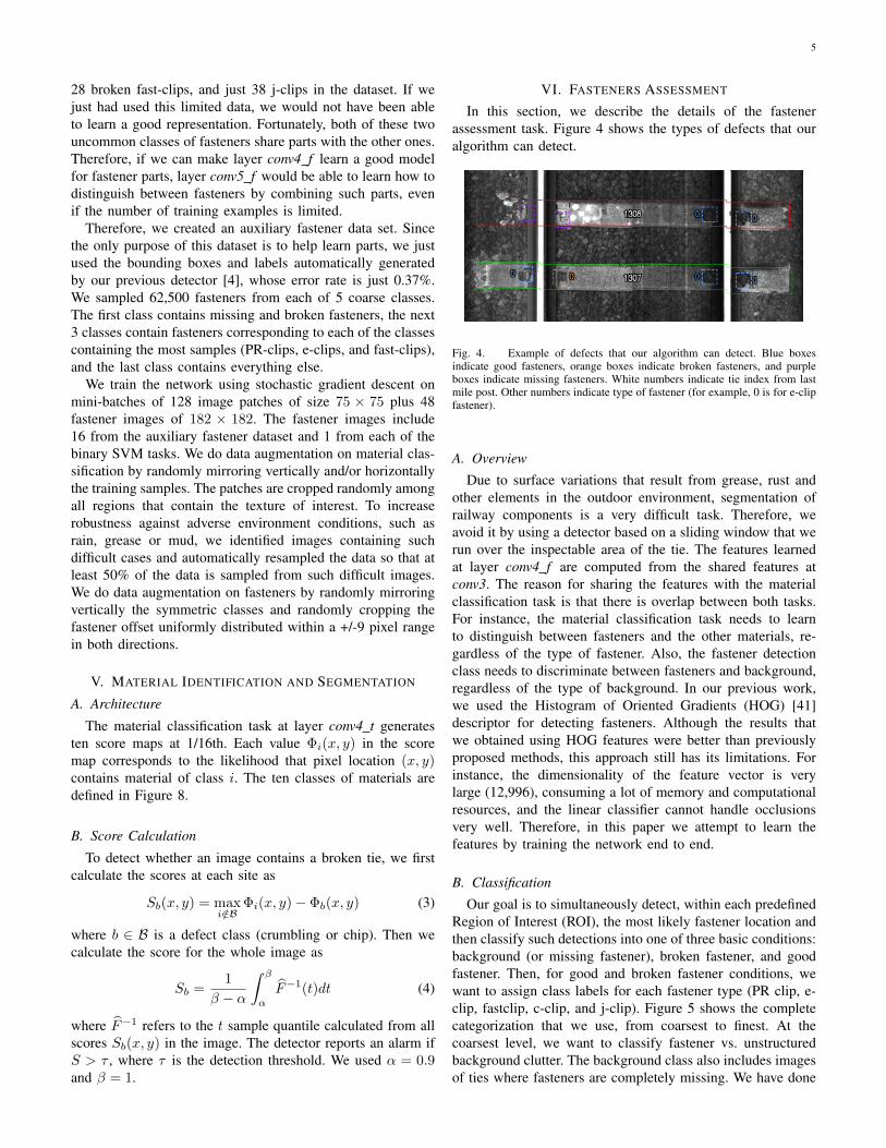
In this section, we describe the details of the fastenerassessment task. Figure 4 shows the types of defects that ouralgorithm can detect.

Fig. 4. Example of defects that our algorithm can detect. Blue boxesindicate good fasteners, orange boxes indicate broken fasteners, and purpleboxes indicate missing fasteners. White numbers indicate tie index from lastmile post. Other numbers indicate type of fastener (for example, 0 is for e-clipfastener).

A. Overview

Due to surface variations that result from grease, rust andother elements in the outdoor environment, segmentation ofrailway components is a very difficult task. Therefore, weavoid it by using a detector based on a sliding window that werun over the inspectable area of the tie. The features learnedat layer conv4 f are computed from the shared features atconv3. The reason for sharing the features with the materialclassification task is that there is overlap between both tasks.For instance, the material classification task needs to learnto distinguish between fasteners and the other materials, re-gardless of the type of fastener. Also, the fastener detectionclass needs to discriminate between fasteners and background,regardless of the type of background. In our previous work,we used the Histogram of Oriented Gradients (HOG) [41]descriptor for detecting fasteners. Although the results thatwe obtained using HOG features were better than previouslyproposed methods, this approach still has its limitations. Forinstance, the dimensionality of the feature vector is verylarge (12,996), consuming a lot of memory and computationalresources, and the linear classifier cannot handle occlusionsvery well. Therefore, in this paper we attempt to learn thefeatures by training the network end to end.

B. Classification

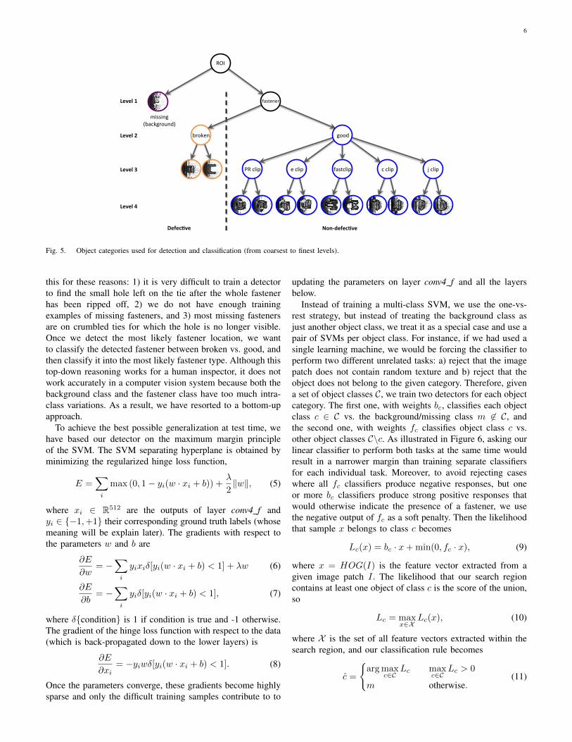
Our goal is to simultaneously detect, within each predefinedRegion of Interest (ROI), the most likely fastener location andthen classify such detections into one of three basic conditions:background (or missing fastener), broken fastener, and goodfastener. Then, for good and broken fastener conditions, wewant to assign class labels for each fastener type (PR clip, e-clip, fastclip, c-clip, and j-clip). Figure 5 shows the completecategorization that we use, from coarsest to finest. At thecoarsest level, we want to classify fastener vs. unstructuredbackground clutter. The background class also includes imagesof ties where fasteners are completely missing. We have done

6

missing  (background)  

broken  

PR  clip   e  clip   fastclip   c  clip   j  clip  

Level  1  

Level  2  

Level  3  

Defec,ve   Non-­‐defec,ve  

Level  4  

good  

fastener  

ROI  

Fig. 5. Object categories used for detection and classification (from coarsest to finest levels).

this for these reasons: 1) it is very difficult to train a detectorto find the small hole left on the tie after the whole fastenerhas been ripped off, 2) we do not have enough trainingexamples of missing fasteners, and 3) most missing fastenersare on crumbled ties for which the hole is no longer visible.Once we detect the most likely fastener location, we wantto classify the detected fastener between broken vs. good, andthen classify it into the most likely fastener type. Although thistop-down reasoning works for a human inspector, it does notwork accurately in a computer vision system because both thebackground class and the fastener class have too much intra-class variations. As a result, we have resorted to a bottom-upapproach.

To achieve the best possible generalization at test time, wehave based our detector on the maximum margin principleof the SVM. The SVM separating hyperplane is obtained byminimizing the regularized hinge loss function,

E =∑i

max (0, 1− yi(w · xi + b)) +λ

2‖w‖, (5)

where xi ∈ R512 are the outputs of layer conv4 f andyi ∈ {−1,+1} their corresponding ground truth labels (whosemeaning will be explain later). The gradients with respect tothe parameters w and b are

∂E

∂w= −

∑i

yixiδ[yi(w · xi + b) < 1] + λw (6)

∂E

∂b= −

∑i

yiδ[yi(w · xi + b) < 1], (7)

where δ{condition} is 1 if condition is true and -1 otherwise.The gradient of the hinge loss function with respect to the data(which is back-propagated down to the lower layers) is

∂E

∂xi= −yiwδ[yi(w · xi + b) < 1]. (8)

Once the parameters converge, these gradients become highlysparse and only the difficult training samples contribute to to

updating the parameters on layer conv4 f and all the layersbelow.

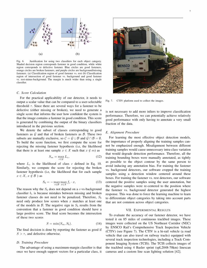
Instead of training a multi-class SVM, we use the one-vs-rest strategy, but instead of treating the background class asjust another object class, we treat it as a special case and use apair of SVMs per object class. For instance, if we had used asingle learning machine, we would be forcing the classifier toperform two different unrelated tasks: a) reject that the imagepatch does not contain random texture and b) reject that theobject does not belong to the given category. Therefore, givena set of object classes C, we train two detectors for each objectcategory. The first one, with weights bc, classifies each objectclass c ∈ C vs. the background/missing class m 6∈ C, andthe second one, with weights fc classifies object class c vs.other object classes C\c. As illustrated in Figure 6, asking ourlinear classifier to perform both tasks at the same time wouldresult in a narrower margin than training separate classifiersfor each individual task. Moreover, to avoid rejecting caseswhere all fc classifiers produce negative responses, but oneor more bc classifiers produce strong positive responses thatwould otherwise indicate the presence of a fastener, we usethe negative output of fc as a soft penalty. Then the likelihoodthat sample x belongs to class c becomes

Lc(x) = bc · x+ min(0, fc · x), (9)

where x = HOG(I) is the feature vector extracted from agiven image patch I . The likelihood that our search regioncontains at least one object of class c is the score of the union,so

Lc = maxx∈X

Lc(x), (10)

where X is the set of all feature vectors extracted within thesearch region, and our classification rule becomes

c =

{arg max

c∈CLc max

c∈CLc > 0

m otherwise.(11)

7

(a) (b)

Fig. 6. Justification for using two classifiers for each object category.Shaded decision region corresponds fastener in good condition, while whiteregion corresponds to defective fastener. Blue circles are good fasteners,orange circles are broken fasteners, and purple circles are background/missingfasteners. (a) Classification region of good fastener vs. rest (b) Classificationregion of intersection of good fastener vs. background and good fastenervs. rest-minus-background. The margin is much wider than using a singleclassifier.

C. Score Calculation

For the practical applicability of our detector, it needs tooutput a scalar value that can be compared to a user-selectablethreshold τ . Since there are several ways for a fastener to bedefective (either missing or broken), we need to generate asingle score that informs the user how confident the system isthat the image contains a fastener in good condition. This scoreis generated by combining the output of the binary classifiersintroduced in the previous section.

We denote the subset of classes corresponding to goodfasteners as G and that of broken fasteners as B. These twosubsets are mutually exclusive, so C = G ∪ B and G ∩ B = ∅.To build the score function, we first compute the score forrejecting the missing fastener hypothesis (i.e, the likelihoodthat there is at least one sample x ∈ X such that x /∈ m) as

Sm = maxc∈G

Lc, (12)

where Lc is the likelihood of class c defined in Eq. 10.Similarly, we compute the score for rejecting the brokenfastener hypothesis (i.e, the likelihood that for each samplex ∈ X , x /∈ B ) as

Sb = −maxc∈B

maxx∈X

fc · x, (13)

The reason why the Sb does not depend on a c-vs-backgroundclassifier bc is because mistakes between missing and brokenfastener classes do not need to be penalized. Therefore, Sbneed only produce low scores when x matches at least oneof the models in B. The negative sign in Sb results from theconvention that a fastener in good condition should have alarge positive score. The final score becomes the intersectionof these two scores

S = min(Sm, Sb). (14)

The final decision is done by reporting the fastener as good ifS > τ , and defective otherwise.

D. Training Procedure

The advantage of using a maximum-margin classifier is thatonce we have enough support vectors for a particular class, it

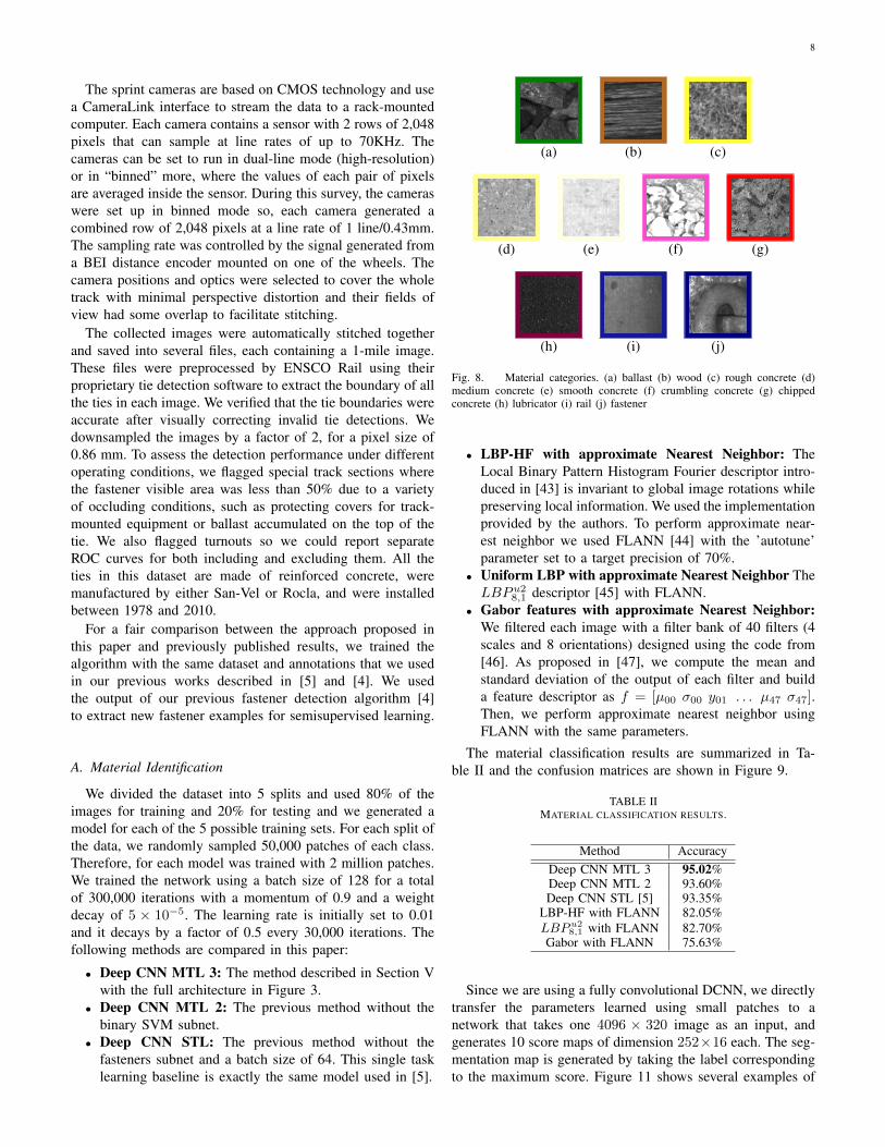
Fig. 7. CTIV platform used to collect the images.

is not necessary to add more inliers to improve classificationperformance. Therefore, we can potentially achieve relativelygood performance with only having to annotate a very smallfraction of the data.

E. Alignment Procedure

For learning the most effective object detection models,the importance of properly aligning the training samples can-not be emphasized enough. Misalignment between differenttraining samples would cause unnecessary intra-class variationthat would degrade detection performance. Therefore, all thetraining bounding boxes were manually annotated, as tightlyas possible to the object contour by the same person toavoid inducing any annotation bias. For training the fastenervs. background detectors, our software cropped the trainingsamples using a detection window centered around theseboxes. For training the fastener vs. rest detectors, our softwarecentered the positive samples using the user annotation, butthe negative samples were re-centered to the position wherethe fastener vs. background detector generated the highestresponse. This was done to force the learning machine to learnto differentiate object categories by taking into account partsthat are not common across object categories.

VII. EXPERIMENTAL RESULTS

To evaluate the accuracy of our fastener detector, we havetested it on 85 miles of continuous trackbed images. Theseimages were collected on the US Northeast Corridor (NEC)by ENSCO Rail’s Comprehensive Track Inspection Vehicle(CTIV) (see Figure 7). The CTIV is a hi-rail vehicle (a roadvehicle that can also travel on railway tracks) equipped withseveral track inspection technologies, including a Track Com-ponent Imaging System (TCIS). The TCIS collects images ofthe trackbed using 4 Basler sprint (spL2048-70km) linescancameras and a custom line scan lighting solution [42].

8

The sprint cameras are based on CMOS technology and usea CameraLink interface to stream the data to a rack-mountedcomputer. Each camera contains a sensor with 2 rows of 2,048pixels that can sample at line rates of up to 70KHz. Thecameras can be set to run in dual-line mode (high-resolution)or in “binned” more, where the values of each pair of pixelsare averaged inside the sensor. During this survey, the cameraswere set up in binned mode so, each camera generated acombined row of 2,048 pixels at a line rate of 1 line/0.43mm.The sampling rate was controlled by the signal generated froma BEI distance encoder mounted on one of the wheels. Thecamera positions and optics were selected to cover the wholetrack with minimal perspective distortion and their fields ofview had some overlap to facilitate stitching.

The collected images were automatically stitched togetherand saved into several files, each containing a 1-mile image.These files were preprocessed by ENSCO Rail using theirproprietary tie detection software to extract the boundary of allthe ties in each image. We verified that the tie boundaries wereaccurate after visually correcting invalid tie detections. Wedownsampled the images by a factor of 2, for a pixel size of0.86 mm. To assess the detection performance under differentoperating conditions, we flagged special track sections wherethe fastener visible area was less than 50% due to a varietyof occluding conditions, such as protecting covers for track-mounted equipment or ballast accumulated on the top of thetie. We also flagged turnouts so we could report separateROC curves for both including and excluding them. All theties in this dataset are made of reinforced concrete, weremanufactured by either San-Vel or Rocla, and were installedbetween 1978 and 2010.

For a fair comparison between the approach proposed inthis paper and previously published results, we trained thealgorithm with the same dataset and annotations that we usedin our previous works described in [5] and [4]. We usedthe output of our previous fastener detection algorithm [4]to extract new fastener examples for semisupervised learning.

A. Material Identification

We divided the dataset into 5 splits and used 80% of theimages for training and 20% for testing and we generated amodel for each of the 5 possible training sets. For each split ofthe data, we randomly sampled 50,000 patches of each class.Therefore, for each model was trained with 2 million patches.We trained the network using a batch size of 128 for a totalof 300,000 iterations with a momentum of 0.9 and a weightdecay of 5 × 10−5. The learning rate is initially set to 0.01and it decays by a factor of 0.5 every 30,000 iterations. Thefollowing methods are compared in this paper:

• Deep CNN MTL 3: The method described in Section Vwith the full architecture in Figure 3.

• Deep CNN MTL 2: The previous method without thebinary SVM subnet.

• Deep CNN STL: The previous method without thefasteners subnet and a batch size of 64. This single tasklearning baseline is exactly the same model used in [5].

(a) (b) (c)

(d) (e) (f) (g)

(h) (i) (j)

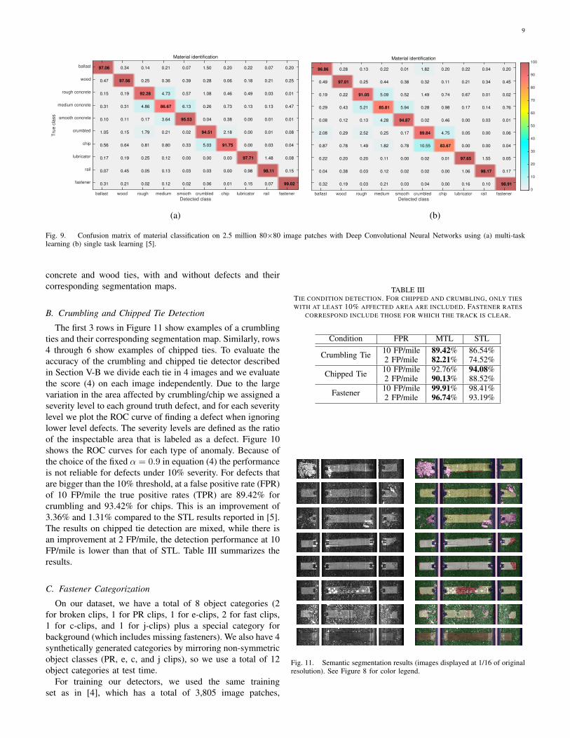
Fig. 8. Material categories. (a) ballast (b) wood (c) rough concrete (d)medium concrete (e) smooth concrete (f) crumbling concrete (g) chippedconcrete (h) lubricator (i) rail (j) fastener

• LBP-HF with approximate Nearest Neighbor: TheLocal Binary Pattern Histogram Fourier descriptor intro-duced in [43] is invariant to global image rotations whilepreserving local information. We used the implementationprovided by the authors. To perform approximate near-est neighbor we used FLANN [44] with the ’autotune’parameter set to a target precision of 70%.

• Uniform LBP with approximate Nearest Neighbor TheLBPu28,1 descriptor [45] with FLANN.

• Gabor features with approximate Nearest Neighbor:We filtered each image with a filter bank of 40 filters (4scales and 8 orientations) designed using the code from[46]. As proposed in [47], we compute the mean andstandard deviation of the output of each filter and builda feature descriptor as f = [µ00 σ00 y01 . . . µ47 σ47].Then, we perform approximate nearest neighbor usingFLANN with the same parameters.

The material classification results are summarized in Ta-ble II and the confusion matrices are shown in Figure 9.

TABLE IIMATERIAL CLASSIFICATION RESULTS.

Method AccuracyDeep CNN MTL 3 95.02%Deep CNN MTL 2 93.60%Deep CNN STL [5] 93.35%

LBP-HF with FLANN 82.05%LBPu2

8,1 with FLANN 82.70%Gabor with FLANN 75.63%

Since we are using a fully convolutional DCNN, we directlytransfer the parameters learned using small patches to anetwork that takes one 4096 × 320 image as an input, andgenerates 10 score maps of dimension 252×16 each. The seg-mentation map is generated by taking the label correspondingto the maximum score. Figure 11 shows several examples of

9

0.47

0.15

0.31

0.10

1.05

0.56

0.17

0.07

0.31

0.34

0.19

0.31

0.11

0.15

0.64

0.19

0.45

0.21

0.14

0.25

4.86

0.17

1.79

0.81

0.25

0.05

0.02

0.21

0.36

4.73

3.64

0.21

0.80

0.12

0.13

0.12

0.07

0.39

0.57

6.13

0.02

0.33

0.00

0.03

0.02

1.50

0.28

1.08

0.26

0.04

5.03

0.00

0.03

0.06

0.20

0.06

0.46

0.73

0.38

2.18

0.00

0.00

0.01

0.22

0.18

0.49

0.13

0.00

0.00

0.00

0.98

0.15

0.07

0.21

0.03

0.13

0.01

0.01

0.03

1.48

0.07

0.20

0.25

0.01

0.47

0.01

0.08

0.04

0.08

0.15

97.06

97.56

92.28

86.67

95.53

94.51

91.75

97.71

98.11

99.02

Material identification

Detected classballast wood rough medium smooth crumbled chip lubricator rail fastener

Tru

e c

lass

ballast

wood

rough concrete

medium concrete

smooth concrete

crumbled

chip

lubricator

rail

fastener

0

10

20

30

40

50

60

70

80

90

100

0.49

0.19

0.29

0.08

2.08

0.87

0.22

0.04

0.32

0.28

0.22

0.43

0.12

0.29

0.78

0.20

0.38

0.19

0.13

0.25

5.21

0.13

2.52

1.49

0.20

0.03

0.03

0.22

0.44

5.09

4.28

0.25

1.82

0.11

0.12

0.21

0.01

0.38

0.52

5.94

0.17

0.78

0.00

0.02

0.03

1.82

0.32

1.49

0.28

0.02

10.55

0.02

0.02

0.04

0.20

0.11

0.74

0.98

0.46

4.75

0.01

0.00

0.00

0.22

0.21

0.67

0.17

0.00

0.05

0.00

1.06

0.16

0.04

0.34

0.01

0.14

0.03

0.00

0.00

1.55

0.10

0.20

0.45

0.02

0.76

0.01

0.06

0.04

0.05

0.17

96.86

97.01

91.05

85.81

94.87

89.84

83.67

97.65

98.17

98.91

Material identification

Detected classballast wood rough medium smooth crumbled chip lubricator rail fastener

Tru

e c

lass

ballast

wood

rough concrete

medium concrete

smooth concrete

crumbled

chip

lubricator

rail

fastener

0

10

20

30

40

50

60

70

80

90

100

(a) (b)

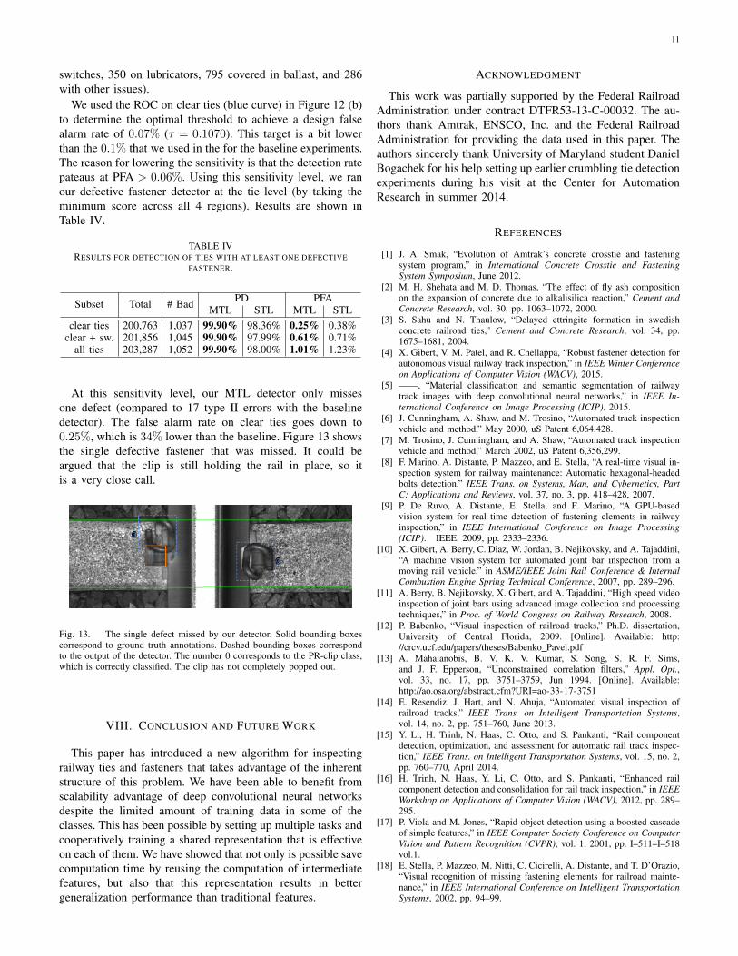
Fig. 9. Confusion matrix of material classification on 2.5 million 80×80 image patches with Deep Convolutional Neural Networks using (a) multi-tasklearning (b) single task learning [5].

concrete and wood ties, with and without defects and theircorresponding segmentation maps.

B. Crumbling and Chipped Tie Detection

The first 3 rows in Figure 11 show examples of a crumblingties and their corresponding segmentation map. Similarly, rows4 through 6 show examples of chipped ties. To evaluate theaccuracy of the crumbling and chipped tie detector describedin Section V-B we divide each tie in 4 images and we evaluatethe score (4) on each image independently. Due to the largevariation in the area affected by crumbling/chip we assigned aseverity level to each ground truth defect, and for each severitylevel we plot the ROC curve of finding a defect when ignoringlower level defects. The severity levels are defined as the ratioof the inspectable area that is labeled as a defect. Figure 10shows the ROC curves for each type of anomaly. Because ofthe choice of the fixed α = 0.9 in equation (4) the performanceis not reliable for defects under 10% severity. For defects thatare bigger than the 10% threshold, at a false positive rate (FPR)of 10 FP/mile the true positive rates (TPR) are 89.42% forcrumbling and 93.42% for chips. This is an improvement of3.36% and 1.31% compared to the STL results reported in [5].The results on chipped tie detection are mixed, while there isan improvement at 2 FP/mile, the detection performance at 10FP/mile is lower than that of STL. Table III summarizes theresults.

C. Fastener Categorization

On our dataset, we have a total of 8 object categories (2for broken clips, 1 for PR clips, 1 for e-clips, 2 for fast clips,1 for c-clips, and 1 for j-clips) plus a special category forbackground (which includes missing fasteners). We also have 4synthetically generated categories by mirroring non-symmetricobject classes (PR, e, c, and j clips), so we use a total of 12object categories at test time.

For training our detectors, we used the same trainingset as in [4], which has a total of 3,805 image patches,

TABLE IIITIE CONDITION DETECTION. FOR CHIPPED AND CRUMBLING, ONLY TIESWITH AT LEAST 10% AFFECTED AREA ARE INCLUDED. FASTENER RATES

CORRESPOND INCLUDE THOSE FOR WHICH THE TRACK IS CLEAR.

Condition FPR MTL STL

Crumbling Tie 10 FP/mile 89.42% 86.54%2 FP/mile 82.21% 74.52%

Chipped Tie 10 FP/mile 92.76% 94.08%2 FP/mile 90.13% 88.52%

Fastener 10 FP/mile 99.91% 98.41%2 FP/mile 96.74% 93.19%

Fig. 11. Semantic segmentation results (images displayed at 1/16 of originalresolution). See Figure 8 for color legend.

10

False Positives per Mile10

-210

-110

010

110

210

310

4

De

tectio

n R

ate

0.3

0.4

0.5

0.6

0.7

0.8

0.9

1Crumbling tie detection

overall (STL)

≥ 10% (STL)≥ 20% (STL)

≥ 30% (STL)≥ 40% (STL)

≥ 50% (STL)≥ 60% (STL)

≥ 70% (STL)overall (MTL)≥ 10% (MTL)≥ 20% (MTL)

≥ 30% (MTL)≥ 40% (MTL)

≥ 50% (MTL)≥ 60% (MTL)

≥ 70% (MTL)

False Positives per Mile10

-210

-110

010

110

210

310

4

De

tectio

n R

ate

0.1

0.2

0.3

0.4

0.5

0.6

0.7

0.8

0.9

1Chipped tie detection

overall (STL)

≥ 10% (STL)≥ 20% (STL)

≥ 30% (STL)≥ 40% (STL)

≥ 50% (STL)≥ 60% (STL)

≥ 70% (STL)overall (MTL)≥ 10% (MTL)≥ 20% (MTL)

≥ 30% (MTL)≥ 40% (MTL)

≥ 50% (MTL)≥ 60% (MTL)

≥ 70% (MTL)

(a) (b)

Fig. 10. (a) ROC curve for detecting crumbling tie conditions. (a) ROC curve for detecting chip tie conditions. Each curve is generated considering conditionsat or above a certain severity level. Note: False positive rates are estimated assuming an average of 104 images per mile. Confusion between chipped andcrumbling defects are not counted as false positives.

PFA0 0.1 0.2 0.3 0.4 0.5 0.6 0.7 0.8 0.9 1

PD

0

0.1

0.2

0.3

0.4

0.5

0.6

0.7

0.8

0.9

1

proposed methodWACV 2015HOG OT-MACHHOG DAG SVMHOG 1-vs-1 vote SVMInt. norm. OT-MACH

PFA0 0.002 0.004 0.006 0.008 0.01 0.012 0.014 0.016 0.018 0.02

PD

0.9

0.91

0.92

0.93

0.94

0.95

0.96

0.97

0.98

0.99

1

proposed methodWACV 2015HOG OT-MACHHOG DAG SVMHOG 1-vs-1 vote SVMInt. norm. OT-MACH

PFA0 0.002 0.004 0.006 0.008 0.01 0.012 0.014 0.016 0.018 0.02

PD

0.9

0.91

0.92

0.93

0.94

0.95

0.96

0.97

0.98

0.99

1

proposed method (clear ties)proposed method (clear ties + sw)proposed method (all ties)WACV 2015 (clear ties)WACV 2015 (clear ties + sw)WACV 2015 (all ties)

(a) (a) detail (b)

Fig. 12. ROC curves for the task of detecting defective (missing or broken) fasteners (a) using 5-fold cross-validation on the training set (b) on the 85-miletesting set.

including 1,069 good fasteners, 714 broken fasteners, 33missing fasteners, and 1,989 patches of background texture.During training, we also included the mirrored versions of themissing/background patches and all symmetric object classes.

In addition to the proposed method described in SectionVI, we have also implemented and evaluated the followingalternative methods:

• STL (WACV 2015): The method in [4] uses the samescores as the proposed method, based on HOG featuresinstead of the features learned at layer conv4 f.

• Intensity normalized OT-MACH: As in [12], for eachimage patch, we subtract the mean and normalize theimage vector to unit norm. For each class c, we designan OT-MACH filter in the Fourier domain using hc =[αI + (1 − α)Dc]

−1xc with α = 0.95, where I is theidentity matrix, Dc = (1/Nc)

∑Nc

i=1 xcix∗ci, and Nc is

the number of training samples of class c.• HOG features with OT-MACH: The method in [12],

but replacing intensity with HOG feature. Since HOGfeatures are already intensity-invariant, the design of thefilters reduces to hc = xc.

• HOG features with DAG-SVM: We run one-vs-oneSVM classifiers in sequence. We first run each classagainst the background on each candidate region. Ifat least one classifier indicates that the patch is notbackground, then we run the DAG-SVM algorithm [48]over the remaining classes.

• HOG features with majority voting SVM: We run all

possible one-vs-one SVM classifiers and select the classwith the maximum number of votes.

For the second and third methods, we calculate the score usingthe formulation introduced in sections VI-B and VI-C, but withbc = hc and fc = hc−

∑i 6=c hi/(C−1). For the forth and last

methods, we first estimate the most likely class in G and in B.Then, we set Sb as the output of the classifier between thesetwo classes, and Sm as the output of the classifier betweenthe background and the most likely class.

We can observe in Figure 12 (a) that the proposed methodis the most accurate, followed by WACV 2015 STL baselineand HOG with OT-MACH method. The other methods performpoorly on this dataset. In the third row of Table III we comparethe fastener detection performance of MTL with the STLbaseline.

D. Defect Detection

To evaluate the performance of our defect detector, wedivided each tie into 4 regions of interest (left field, left gage,right gage, right field) and calculated the score defined by(14) for each of them. Figure 12 shows the ROC curve forcrossvalidation on the training set as well as for the testingset of 813,148 ROIs (203,287 ties). The testing set contains1,052 ties images with at least one defective fastener per tie.The total number of defective fasteners in the testing set was1,087 (0.13% of all the fasteners), including 22 completelymissing fasteners and 1,065 broken fasteners. The number ofties that we flagged as “uninspectable” is 2,524 (1,093 on

11

switches, 350 on lubricators, 795 covered in ballast, and 286with other issues).

We used the ROC on clear ties (blue curve) in Figure 12 (b)to determine the optimal threshold to achieve a design falsealarm rate of 0.07% (τ = 0.1070). This target is a bit lowerthan the 0.1% that we used in the for the baseline experiments.The reason for lowering the sensitivity is that the detection ratepateaus at PFA > 0.06%. Using this sensitivity level, we ranour defective fastener detector at the tie level (by taking theminimum score across all 4 regions). Results are shown inTable IV.

TABLE IVRESULTS FOR DETECTION OF TIES WITH AT LEAST ONE DEFECTIVE

FASTENER.

Subset Total # Bad PD PFAMTL STL MTL STL

clear ties 200,763 1,037 99.90% 98.36% 0.25% 0.38%clear + sw. 201,856 1,045 99.90% 97.99% 0.61% 0.71%

all ties 203,287 1,052 99.90% 98.00% 1.01% 1.23%

At this sensitivity level, our MTL detector only missesone defect (compared to 17 type II errors with the baselinedetector). The false alarm rate on clear ties goes down to0.25%, which is 34% lower than the baseline. Figure 13 showsthe single defective fastener that was missed. It could beargued that the clip is still holding the rail in place, so itis a very close call.

Fig. 13. The single defect missed by our detector. Solid bounding boxescorrespond to ground truth annotations. Dashed bounding boxes correspondto the output of the detector. The number 0 corresponds to the PR-clip class,which is correctly classified. The clip has not completely popped out.

VIII. CONCLUSION AND FUTURE WORK

This paper has introduced a new algorithm for inspectingrailway ties and fasteners that takes advantage of the inherentstructure of this problem. We have been able to benefit fromscalability advantage of deep convolutional neural networksdespite the limited amount of training data in some of theclasses. This has been possible by setting up multiple tasks andcooperatively training a shared representation that is effectiveon each of them. We have showed that not only is possible savecomputation time by reusing the computation of intermediatefeatures, but also that this representation results in bettergeneralization performance than traditional features.

ACKNOWLEDGMENT

This work was partially supported by the Federal RailroadAdministration under contract DTFR53-13-C-00032. The au-thors thank Amtrak, ENSCO, Inc. and the Federal RailroadAdministration for providing the data used in this paper. Theauthors sincerely thank University of Maryland student DanielBogachek for his help setting up earlier crumbling tie detectionexperiments during his visit at the Center for AutomationResearch in summer 2014.

REFERENCES

[1] J. A. Smak, “Evolution of Amtrak’s concrete crosstie and fasteningsystem program,” in International Concrete Crosstie and FasteningSystem Symposium, June 2012.

[2] M. H. Shehata and M. D. Thomas, “The effect of fly ash compositionon the expansion of concrete due to alkalisilica reaction,” Cement andConcrete Research, vol. 30, pp. 1063–1072, 2000.

[3] S. Sahu and N. Thaulow, “Delayed ettringite formation in swedishconcrete railroad ties,” Cement and Concrete Research, vol. 34, pp.1675–1681, 2004.

[4] X. Gibert, V. M. Patel, and R. Chellappa, “Robust fastener detection forautonomous visual railway track inspection,” in IEEE Winter Conferenceon Applications of Computer Vision (WACV), 2015.

[5] ——, “Material classification and semantic segmentation of railwaytrack images with deep convolutional neural networks,” in IEEE In-ternational Conference on Image Processing (ICIP), 2015.

[6] J. Cunningham, A. Shaw, and M. Trosino, “Automated track inspectionvehicle and method,” May 2000, uS Patent 6,064,428.

[7] M. Trosino, J. Cunningham, and A. Shaw, “Automated track inspectionvehicle and method,” March 2002, uS Patent 6,356,299.

[8] F. Marino, A. Distante, P. Mazzeo, and E. Stella, “A real-time visual in-spection system for railway maintenance: Automatic hexagonal-headedbolts detection,” IEEE Trans. on Systems, Man, and Cybernetics, PartC: Applications and Reviews, vol. 37, no. 3, pp. 418–428, 2007.

[9] P. De Ruvo, A. Distante, E. Stella, and F. Marino, “A GPU-basedvision system for real time detection of fastening elements in railwayinspection,” in IEEE International Conference on Image Processing(ICIP). IEEE, 2009, pp. 2333–2336.

[10] X. Gibert, A. Berry, C. Diaz, W. Jordan, B. Nejikovsky, and A. Tajaddini,“A machine vision system for automated joint bar inspection from amoving rail vehicle,” in ASME/IEEE Joint Rail Conference & InternalCombustion Engine Spring Technical Conference, 2007, pp. 289–296.

[11] A. Berry, B. Nejikovsky, X. Gibert, and A. Tajaddini, “High speed videoinspection of joint bars using advanced image collection and processingtechniques,” in Proc. of World Congress on Railway Research, 2008.

[12] P. Babenko, “Visual inspection of railroad tracks,” Ph.D. dissertation,University of Central Florida, 2009. [Online]. Available: http://crcv.ucf.edu/papers/theses/Babenko Pavel.pdf

[13] A. Mahalanobis, B. V. K. V. Kumar, S. Song, S. R. F. Sims,and J. F. Epperson, “Unconstrained correlation filters,” Appl. Opt.,vol. 33, no. 17, pp. 3751–3759, Jun 1994. [Online]. Available:http://ao.osa.org/abstract.cfm?URI=ao-33-17-3751

[14] E. Resendiz, J. Hart, and N. Ahuja, “Automated visual inspection ofrailroad tracks,” IEEE Trans. on Intelligent Transportation Systems,vol. 14, no. 2, pp. 751–760, June 2013.

[15] Y. Li, H. Trinh, N. Haas, C. Otto, and S. Pankanti, “Rail componentdetection, optimization, and assessment for automatic rail track inspec-tion,” IEEE Trans. on Intelligent Transportation Systems, vol. 15, no. 2,pp. 760–770, April 2014.

[16] H. Trinh, N. Haas, Y. Li, C. Otto, and S. Pankanti, “Enhanced railcomponent detection and consolidation for rail track inspection,” in IEEEWorkshop on Applications of Computer Vision (WACV), 2012, pp. 289–295.

[17] P. Viola and M. Jones, “Rapid object detection using a boosted cascadeof simple features,” in IEEE Computer Society Conference on ComputerVision and Pattern Recognition (CVPR), vol. 1, 2001, pp. I–511–I–518vol.1.

[18] E. Stella, P. Mazzeo, M. Nitti, C. Cicirelli, A. Distante, and T. D’Orazio,“Visual recognition of missing fastening elements for railroad mainte-nance,” in IEEE International Conference on Intelligent TransportationSystems, 2002, pp. 94–99.

12

[19] F. Marino, A. Distante, P. L. Mazzeo, and E. Stella, “A real-time visualinspection system for railway maintenance: automatic hexagonal-headedbolts detection,” IEEE Trans. on Systems, Man, and Cybernetics, PartC: Applications and Reviews, vol. 37, no. 3, pp. 418–428, 2007.

[20] M. Singh, S. Singh, J. Jaiswal, and J. Hempshall, “Autonomous rail trackinspection using vision based system,” in IEEE International Conferenceon Computational Intelligence for Homeland Security and PersonalSafety, Oct 2006, pp. 56–59.

[21] H.-Y. Hsieh, N. Chen, and C.-L. Liao, “Visual recognition systemof elastic rail clips for mass rapid transit systems,” in ASME/IEEEJoint Rail Conference & Internal Combustion Engine Spring TechnicalConference, 2007, pp. 319–325.

[22] Y. Xia, F. Xie, and Z. Jiang, “Broken railway fastener detection based onadaboost algorithm,” in IEEE International Conference on Optoelectron-ics and Image Processing (ICOIP), vol. 1. IEEE, 2010, pp. 313–316.

[23] J. Yang, W. Tao, M. Liu, Y. Zhang, H. Zhang, and H. Zhao, “An efficientdirection field-based method for the detection of fasteners on high-speedrailways,” Sensors, vol. 11, no. 8, pp. 7364–7381, 2011.

[24] H. Feng, Z. Jiang, F. Xie, P. Yang, J. Shi, and L. Chen, “Automaticfastener classification and defect detection in vision-based railwayinspection systems,” IEEE Trans. on Instrumentation and Measurement,vol. 63, no. 4, pp. 877–888, April 2014.

[25] X. Gibert, V. M. Patel, D. Labate, and R. Chellappa, “Discrete shearlettransform on GPU with applications in anomaly detection and denois-ing,” EURASIP Journal on Advances in Signal Processing, vol. 2014,no. 64, pp. 1–14, May 2014.

[26] R. Khan, S. Islam, and R. Biswas, “Automatic detection of defectiverail anchors,” in IEEE 17th International Conference on IntelligentTransportation Systems (ITSC), Oct 2014, pp. 1583–1588.

[27] K. Fukushima, “Neocognitron: A self-organizing neural network modelfor a mechanism of pattern recognition unaffected by shift in position,”Biological Cybernetics, vol. 36, no. 4, pp. 93–202, 1980.

[28] Y. LeCun, B. Boser, J. S. Denker, D. Henderson, R. E. Howard,W. Hubbard, and L. D. Jackel, “Backpropagation applied to handwrittenzip code recognition,” Neural Computation, vol. 1, no. 4, pp. 541–551,1989.

[29] Y. LeCun, L. Bottou, Y. Bengio, and P. Haffner, “Gradient-based learningapplied to document recognition,” Proceedings of the IEEE, November1998.

[30] A. Krizhevsky, I. Sutskever, and G. E. Hinton, “Imagenet classificationwith deep convolutional neural networks,” in Advances in Neural Infor-mation Systems (NIPS), 2013.

[31] C. Szegedy, W. Liu, Y. Jia, P. Sermanet, S. Reed, D. Anguelov, D. Erhan,V. Vanhoucke, and A. Rabinovich, “Going deeper with convolutions,” inIEEE Conference on Computer Vision and Pattern Recognition (CVPR),June 2015.

[32] R. Girshick, J. Donahue, T. Darrell, and J. Malik, “Rich featurehierarchies for accurate object detection and semantic segmentation,” inIEEE Conference on Computer Vision and Pattern Recognition (CVPR),2014.

[33] Y. Jia, E. Shelhamer, J. Donahue, S. Karayev, J. Long, R. Girshick,S. Guadarrama, and T. Darrell, “Caffe: Convolutional architecture forfast feature embedding,” arXiv:1408.5093, 2014.

[34] R. Collobert, K. Kavukcuoglu, and C. Farabet, “Torch7: A matlab-likeenvironment for machine learning,” in Advances in Neural InformationSystems (NIPS), 2011.

[35] J. Long, E. Shelhamer, and T. Darrell, “Fully convolutional networks forsemantic segmentation,” in IEEE Conference on Computer Vision andPattern Recognition (CVPR), June 2015.

[36] R. Caruana, “Multitask learning,” Machine Learning, vol. 28, no. 1, pp.41–75, Jul 1997.

[37] L. Y. Pratt, J. Mostow, and C. A. Kamm, “Direct transfer of learnedinformation among neural networks,” in Proc. Of AAAI, 1991.

[38] G. Hinton, “Learning distributed representation of concepts,” in Proc.of the 8th Int. Conf. of the Cognitive Science Society, 1986, pp. 1–12.

[39] L. Fei-Fei, R. Fergus, and P. Perona, “One-shot learning of objectcategories,” IEEE Trans. Pattern Analysis and Machine Intelligence,vol. 28, pp. 594–611, 2006.

[40] G. E. Hinton, N. Srivastava, A. Krizhevsky, I. Sutskever, and R. R.Salakhutdinov, “Improving neural networks by preventing co-adaptationof feature detectors,” arXiv preprint arXiv:1207.0580, 2012.

[41] N. Dalal and B. Triggs, “Histograms of oriented gradients for humandetection,” in IEEE Computer Society Conference on Computer Visionand Pattern Recognition (CVPR), vol. 1, Jun 2005, pp. 886–893.

[42] Basler AG, “Success story: ENSCO deploys Basler sprint andace GigE cameras for comprehensive railway track inspection,”

http://www.baslerweb.com/linklist/9/8/3/6/BAS1110 Ensco RailwayInspection.pdf, Oct 2011.

[43] T. Ahonen, J. Matas, C. He, and M. Pietikainen, “Rotation invariantimage description with local binary pattern histogram fourier features,”in Image Analysis. Springer, 2009, pp. 61–70.

[44] M. Muja and D. Lowe, “Fast approximate nearest neighbors withautomatic algorithm configuration,” in International Conference onComputer Vision Theory and Application VISSAPP’09). INSTICCPress, 2009, pp. 331–340.

[45] T. Ojala, M. Pietikainen, and T. Maenpaa, “Multiresolution gray-scaleand rotation invariant texture classification with local binary patterns,”IEEE Trans. on Pattern Analysis and Machine Intelligence, vol. 24,no. 7, pp. 971–987, 2002.

[46] M. Haghighat, S. Zonouz, and M. Abdel-Mottaleb, “Identification usingencrypted biometrics,” in Computer Analysis of Images and Patterns.Springer, 2013, pp. 440–448.

[47] B. Manjunath and W. Ma, “Texture features for browsing and retrieval ofimage data,” IEEE Trans. on Pattern Analysis and Machine Intelligence,vol. 18, no. 8, pp. 837–842, 1996.

[48] J. C. Platt, N. Cristianini, and J. Shawe-taylor, “Large margin DAGs formulticlass classification,” in Advances in Neural Information Systems(NIPS). MIT Press, 2000, pp. 547–553.