deep learning models€“ geoff hinton hasreadingsfrom last year’s nips tutorial. • more papers...
TRANSCRIPT
Deep Learning models
Jie Chen

Course Information
• Class link:– https://noppa.oulu.fi/noppa/kurssi/521010j/etusivu– Slides for Lecture 1 online

Questions
• If I increase x by h, how would the output of f change?
– I+h: image + noise
– w+h: weight update
derivative

Questions
• f =1 ??– E.g., a label for image x (dog, cat, bike)
• Why we do it like this?– Z: weight, we updated weights for each iteration

Back ground
• ANN• Sparse coding• Supervised learning • Unsupervised learning• Shallow Learning & Deep Learning

Sparse coding
• Local feature– A sample x can be represented by
• 64 edge basis • Only 3 of them are non‐zero, using the weights 0.8, 0.3, 0.5. • The weights for the rest basis is 0
Neuroscience Foundation
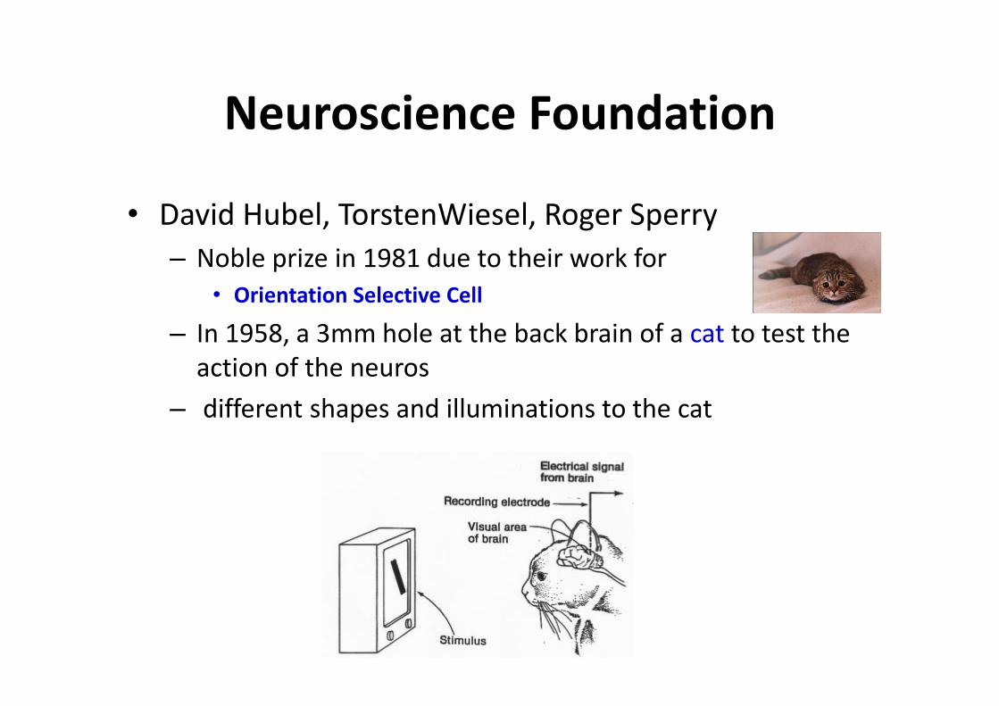
• David Hubel, TorstenWiesel, Roger Sperry– Noble prize in 1981 due to their work for
• Orientation Selective Cell
– In 1958, a 3mm hole at the back brain of a cat to test the action of the neuros
– different shapes and illuminations to the cat

Computer vision
• B. Olshausen, D. Field – Black‐white images in 1995 – S[i], i = 0,.. 399,
• 400 patches size of 16x16
– T, a patch randomly size of 16x16– question:
• Select a group of patches, S[k], • ∑ (a[k] ∗ S[k]) T• The number of S[k] is small as possible

Sparse coding
• Iterations ( (a[k] S[k]) T)– Fix S[k], change a[k]– fix a[k], change S’[k]
• S[k] – Similar edges but in different orientations
• Gabor, 5*8
Back ground
• ANN• Sparse coding• Supervised learning • Unsupervised learning• Shallow Learning & Deep Learning

Supervised learning
– samples: (X, Y)– Regression:
• Y is a real vector• Fit (X, Y) as a curve to minimize the cost function
– Classification:• Y is the class label• Cost function L(X,Y)
, where fi(X)=P(Y=i| X);

Unsupervised learning
• Dataset: X={xi}– Learn a function f to represent the possibilty of P(x)
– density estimation
– Clustering• K‐Means
Back ground
• ANN• Sparse coding• Supervised learning • Unsupervised learning• Shallow Learning & Deep Learning

Shallow Learning & Deep Learning
• Shallow Learning is the first progress of machine learing– Multi‐layer Perceptron– Support Vector Machines (SVM)– Boosting– Maximum entropy (Logistic Regression)
• Deep Learning is the second progress – Geoffrey Hinton, Science 2006
Deep Learning
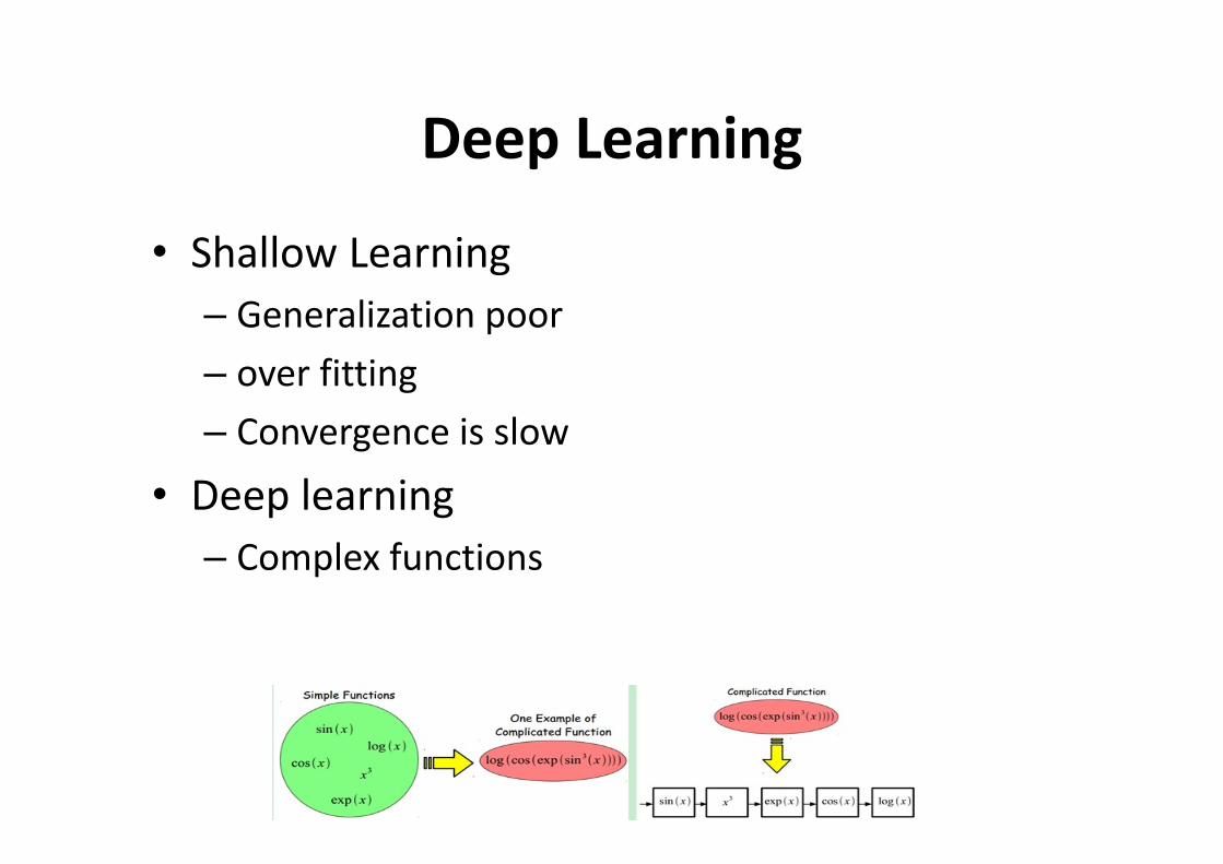
• Shallow Learning– Generalization poor– over fitting– Convergence is slow
• Deep learning– Complex functions
Deep Learning
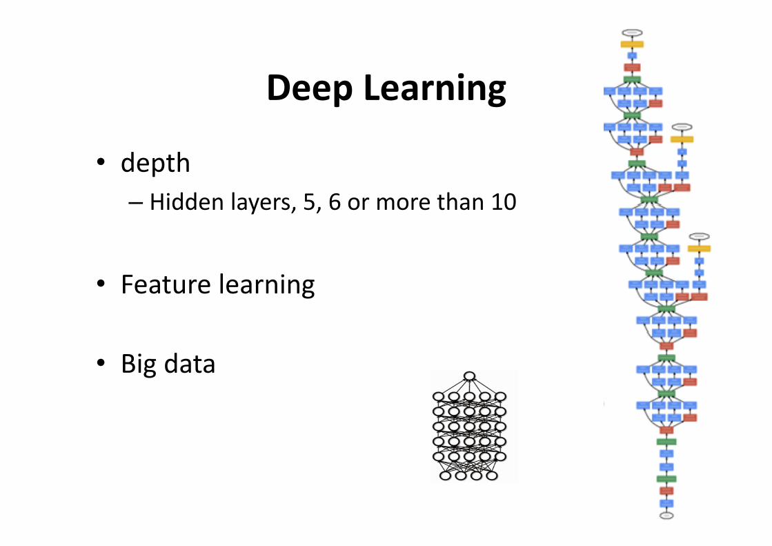
• depth– Hidden layers, 5, 6 or more than 10
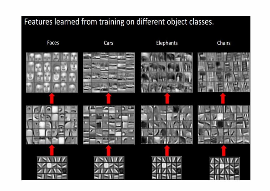
• Feature learning
• Big data

Deep Learning model
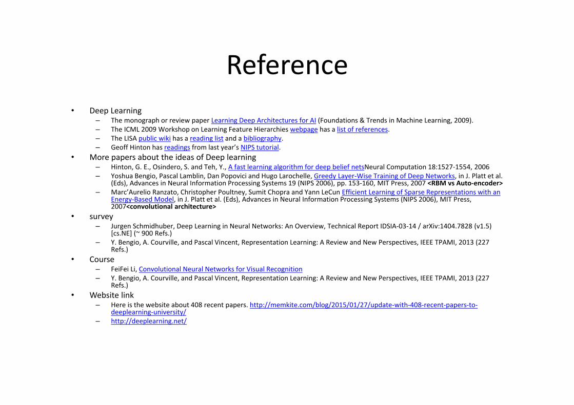
• AutoEncoder• Restricted Boltzmann Machine (RBM)• Deep Belief Networks (DBN)• Convolutional Neural Networks (CNN)

Auto Encoder
• Unsurprised feature learning
– How much layers
– How to perform the unsurprised feature learning
Auto Encoder• Unsurprised feature learning
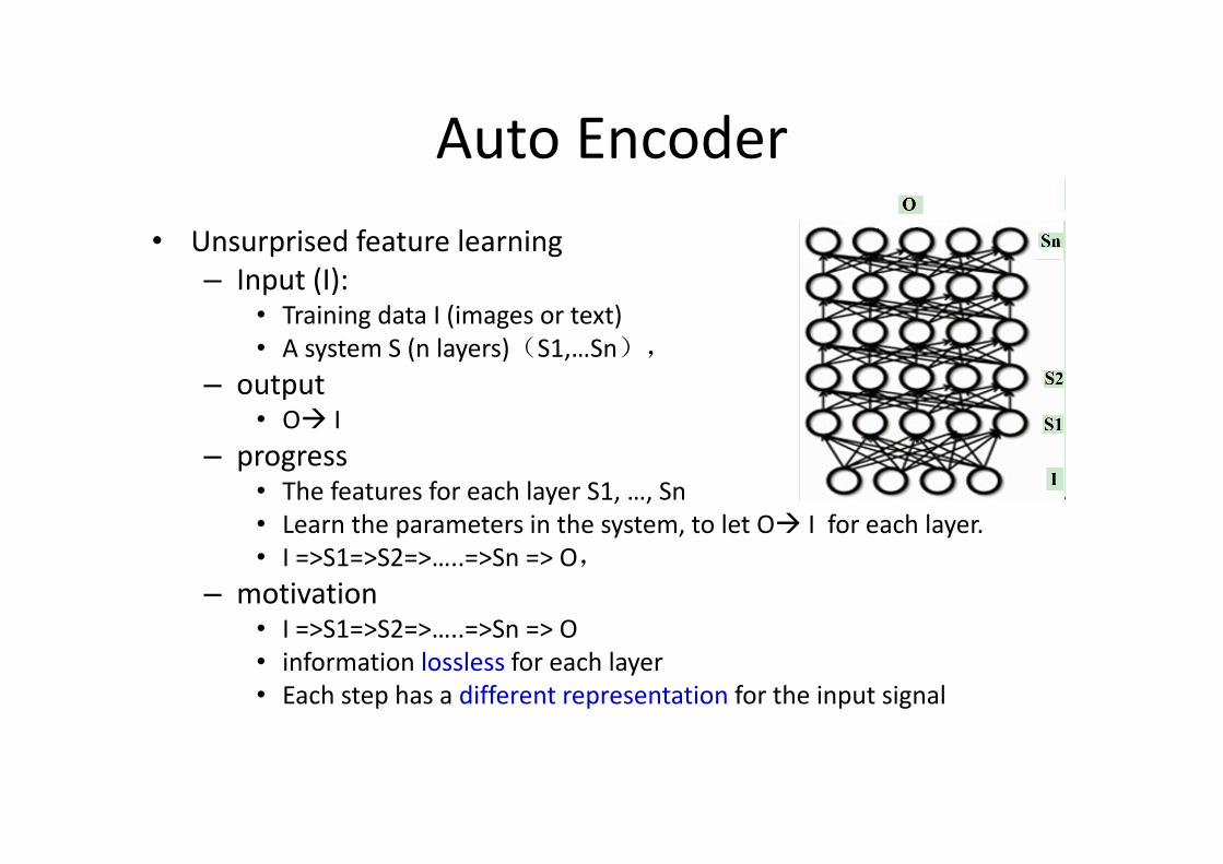
– Input (I):• Training data I (images or text)• A system S (n layers)(S1,…Sn),
– output• O I
– progress• The features for each layer S1, …, Sn• Learn the parameters in the system, to let O I for each layer. • I =>S1=>S2=>…..=>Sn => O,
– motivation• I =>S1=>S2=>…..=>Sn => O• information lossless for each layer• Each step has a different representation for the input signal
Auto Encoder
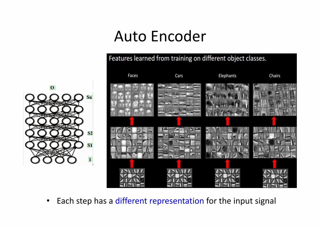
• Each step has a different representation for the input signal

Auto Encoder
• pre‐train– Train one layer in unsupervised way every time– The output of the former layer is the input of the higher layer
• fine‐tuning– Tune the parameters in supervised way– r x’
• x : the original signal • r : the representation from the original signal x • x’ generated by the representation r

Auto Encoder• Unsupervised feature learning from low level to high level
• Feature can be used to represent the input in large dataset.
• Combine the feature and classifier in one framework
Conclusion• Unsupervised feature learning from low level to high level
• Feature can be used to represent the input in large dataset.
• Combine the feature and classifier in one framework
Reference• Deep Learning
– The monograph or review paper Learning Deep Architectures for AI (Foundations & Trends in Machine Learning, 2009).– The ICML 2009 Workshop on Learning Feature Hierarchies webpage has a list of references.– The LISA public wiki has a reading list and a bibliography.– Geoff Hinton has readings from last year’s NIPS tutorial.
• More papers about the ideas of Deep learning– Hinton, G. E., Osindero, S. and Teh, Y., A fast learning algorithm for deep belief netsNeural Computation 18:1527‐1554, 2006– Yoshua Bengio, Pascal Lamblin, Dan Popovici and Hugo Larochelle, Greedy Layer‐Wise Training of Deep Networks, in J. Platt et al.
(Eds), Advances in Neural Information Processing Systems 19 (NIPS 2006), pp. 153‐160, MIT Press, 2007 <RBM vs Auto‐encoder>– Marc’Aurelio Ranzato, Christopher Poultney, Sumit Chopra and Yann LeCun Efficient Learning of Sparse Representations with an
Energy‐Based Model, in J. Platt et al. (Eds), Advances in Neural Information Processing Systems (NIPS 2006), MIT Press, 2007<convolutional architecture>
• survey– Jurgen Schmidhuber, Deep Learning in Neural Networks: An Overview, Technical Report IDSIA‐03‐14 / arXiv:1404.7828 (v1.5)
[cs.NE] (~ 900 Refs.)– Y. Bengio, A. Courville, and Pascal Vincent, Representation Learning: A Review and New Perspectives, IEEE TPAMI, 2013 (227
Refs.)• Course
– FeiFei Li, Convolutional Neural Networks for Visual Recognition– Y. Bengio, A. Courville, and Pascal Vincent, Representation Learning: A Review and New Perspectives, IEEE TPAMI, 2013 (227
Refs.)• Website link
– Here is the website about 408 recent papers. http://memkite.com/blog/2015/01/27/update‐with‐408‐recent‐papers‐to‐deeplearning‐university/
– http://deeplearning.net/

Deep Learning tools• Caffe CNN
– http://caffe.berkeleyvision.org/– a framework for convolutional neural network algorithms.– provides seamless switching between CPU and GPU– fits industry needs
• Matconvnet– http://www.vlfeat.org/matconvnet/)
• Torch– http://torch.ch/
• Theano– a Python library that allows you to define, optimize, and evaluate
mathematical expressions involving multi‐dimensional arrays efficiently.• Matlab For Science Paper
– A deep autoencoder on MNIST digits by Hinton– http://www.cs.toronto.edu/~hinton/MatlabForSciencePaper.html
• AutoEncoder• Restricted Boltzmann Machine (RBM)• Deep Belief Networks (DBN)• Convolutional Neural Networks (CNN)

Background
• Generative model– Model the distribution of input as well as output ,P(x , y)
• Discriminative model– Model the posterior probabilities ,P(y | x)
P(x,y1) P(x,y2) P(y1|x) P(y2|x)
27
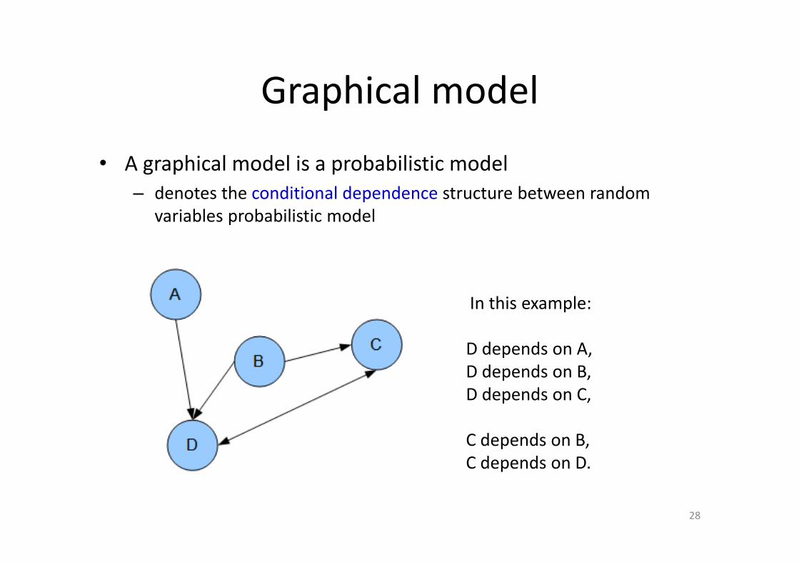
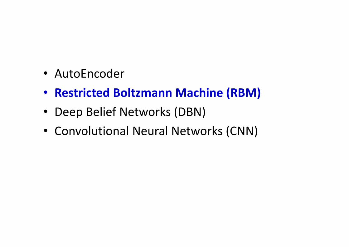
Graphical model
• A graphical model is a probabilistic model – denotes the conditional dependence structure between random
variables probabilistic model
28
In this example:
D depends on A, D depends on B, D depends on C,
C depends on B, C depends on D.

Graphical model
• Directed graphical model
• Undirected graphical model
29
A
B C
D
A
B
C
D
, , ,1∗ φ , , ∗ , ,
, , , | ,

Boltzmann machine
• A graphical representation– Each undirected edge represents dependency.
3 hidden units and 4 visible units. not a restricted Boltzmann machine.
3 hidden units and 2 visible units. a restricted Boltzmann machine.
hidden
i
j
visible
wij
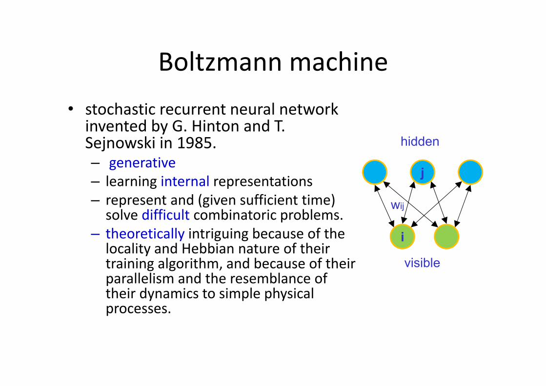
Boltzmann machine• stochastic recurrent neural network invented by G. Hinton and T. Sejnowski in 1985.– generative – learning internal representations – represent and (given sufficient time) solve difficult combinatoric problems.
– theoretically intriguing because of the locality and Hebbian nature of their training algorithm, and because of their parallelism and the resemblance of their dynamics to simple physical processes.
hidden
i
j
visible
wij

Boltzmann machine
• the probability that the i‐th unit is on
hidden
i
j
visible
wij

Boltzmann machine
• Stochastic binary units, and global energy, E:hidden
i
j
visible
wij

Boltzmann machine‐Training• Two kinds of units
– 'visible' units, V, and 'hidden' units, H. – The visible units training set,
• a set of binary vectors over the set V. – The distribution over the training set is denoted
(V).
• The distribution over global states converges as the Boltzmann machine reaches thermal equilibrium. We denote this distribution as
(V) by marginalizing it over the hidden units,
• Our goal is to approximate the "real" distribution (V) using the (V).
hidden
i
j
visible
wij

Boltzmann machine• Measure similarity
• the gradient with respect to a given weight, ,
• , the probability of units i and j both being on when the machine is at equilibrium on the positive phase.
• , is the probability of units i and j both being on when the machine is at equilibrium on the negative phase.
• R denotes the learning rate

Boltzmann machine• Equilibrium state
– run by repeatedly choosing a unit and setting its state according to the below formula.
– After running for long enough at a certain temperature, the probability of a global state of the network will depend only upon that global state's energy, and not on the initial state from which the process was started.
– This relationship is true when the machine is "at thermal equilibrium", meaning that the probability distribution of global states has converged.
– If we start running the network from a high temperature, and gradually decrease it until we reach a thermal equilibrium at a lowtemperature, we may converge to a distribution where the energy level fluctuates around the global minimum. This process is called simulated annealing.

Stochastic SearchWhy BM?
Different optimization criteria in traditional networks and RBM for optimization purpose:
Traditional: Error criterion. BP method strictly goes along the gradient descent direction. Any direction that enlarge error is NOT acceptable. Easy to get stuck in local minima.
BM: associate the network with “Energy”. Simulated Annealing enables the energy to grow under certain probability.

Restricted Boltzmann machines
• Restricted Boltzmann machines (RBM) are unsupervised nonlinear feature learners based on a probabilistic model.
• The features extracted by an RBM or a hierarchy of RBMs often give good results when fed into a linear classifier such as a linear SVM or a perceptron.
Restricted Boltzmann machines
• users to rate a set of movies– explain each movie and user in terms of a set of latent factors.
• movies like Star Wars and Lord of the a latent science fiction and fantasy factor
• users who like Wall‐E and Toy Story might have strong associations with a latent Pixar factor.
– users simply tell you whether they like a movie or not• RBM essentially perform a binary version of factor analysis. – discover latent factors that can explain the activation of these movie choices.
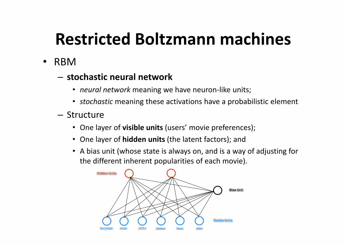
Restricted Boltzmann machines• RBM
– stochastic neural network• neural networkmeaning we have neuron‐like units; • stochasticmeaning these activations have a probabilistic element
– Structure• One layer of visible units (users’ movie preferences);• One layer of hidden units (the latent factors); and• A bias unit (whose state is always on, and is a way of adjusting for the different inherent popularities of each movie).

Restricted Boltzmann machines
• Full connection– each visible/ hidden unit is connected to all the hidden/visible units – bias unit is connected to all the visible and hidden units. – undirected
• Restriction– no visible unit is connected to any other visible unit– So for hidden unit
• To make learning easier
Restricted Boltzmann machines
• example– six movies
• Harry Potter, Avatar, LOTR 3, Gladiator, Titanic, and Glitter
– users tell which ones they want to watch – learn two latent units underlying movie preferences
• SF/fantasy (containing Harry Potter, Avatar, and LOTR 3) • Oscar winners (containing LOTR 3, Gladiator, and Titanic),
– our latent units correspond to these categories

Restricted Boltzmann machines
• RBM: binary‐valued hidden and visible units• Weights
– (size m×n) : hj and vi– ai : bias weights (offsets) for the visible units – bj for the hidden units.
• Energy of a configuration (v,h) is defined as
• Matrix notationiji
i jjj
jji
ii vwhhbvahvE ,),(
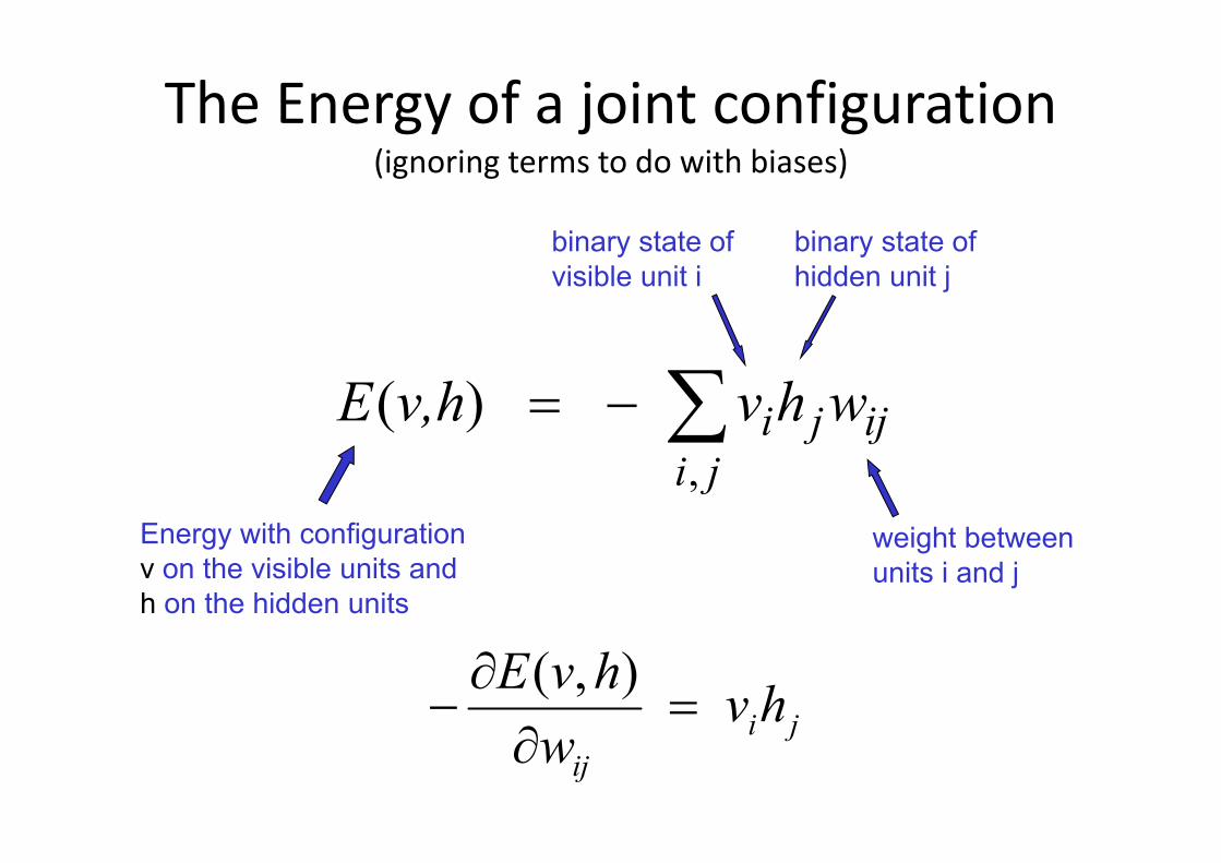
The Energy of a joint configuration(ignoring terms to do with biases)
ji
ijji whvv,hE,
)(
weight between units i and j
Energy with configuration v on the visible units and h on the hidden units
binary state of visible unit i
binary state of hidden unit j
jiij
hvwhvE
),(

Restricted Boltzmann machines
• Probability distributions over hidden and/or visible vectors:
– where Z is a normalizing constant to ensure the probability distribution sums to 1
• Marginal probability of a visible (input) vector of booleans is the sum over all possible hidden layer configurations

Restricted Boltzmann machines
• Conditional probability of h given v
• Individual activation probabilities
– denotes the logistic sigmoid.
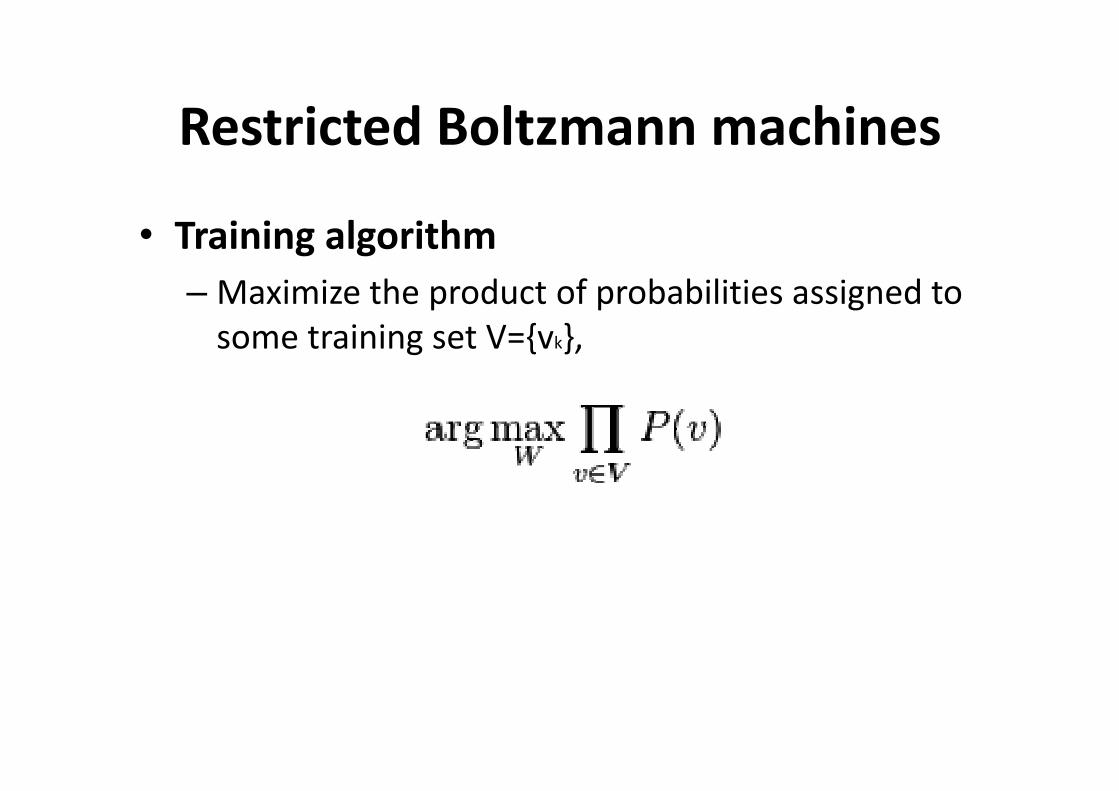
Restricted Boltzmann machines
• Training algorithm– Maximize the product of probabilities assigned to some training set V={vk},

Restricted Boltzmann machines
• CD‐1: Single‐step contrastive divergence– Take a training sample v, compute the probabilities of the hidden units
and sample a hidden activation vector h from this probability distribution.• Compute the outer product of v and h and call this the positive gradient.
– From h, sample a reconstruction v' of the visible units, then resample the hidden activations h' from this. (Gibbs sampling step)
• Compute the outer product of v' and h' and call this the negative gradient.
– update the weight wi,j
ε: learning rate.
• The update rule for the biases a, b is defined analogously.

Deep Boltzmann Machine• Unsupervised feature learning

• Pretraining a DBM with three hidden layers – learning a stack of RBMs.
R. Salakhutdinov, G. Hinton, An Efficient Learning Procedure for Deep Boltzmann Machines, Neural Computation, 2012Hinton, G. E. (2007). To recognize shapes, first learn to generate images. Computational neuroscience: Theoretical insights into brain function. NewYork: Elsevier.

Deep Boltzman Machines
• fine‐tuning– Discriminative
• backpropagation
– Generative • Positive phase: variationalapproximation (mean‐field)
• Negative phase: persistent chain (stochastic approxiamtion)
Salakhutdinov et al, AISTATS 2009, Lee et al, ICML 2009

• AutoEncoder• Restricted Boltzmann Machine (RBM)• Deep Belief Networks (DBN)• Convolutional Neural Networks (CNN)

Belief nets
• A belief net is a directed acyclic graph composed of stochastic variables
53
stochastic hidden causes
visible
Stochastic binary neurons
ii
i wxbz ze
yp
1
1)1(
It is sigmoid belief nets

Belief nets
• we would like to solve two problems– The inference problem: Infer the states of the unobserved variables.– The learning problem: Adjust the interactions between variables to
make the network more likely to generate the training data.
54
stochastic hidden causes
visible
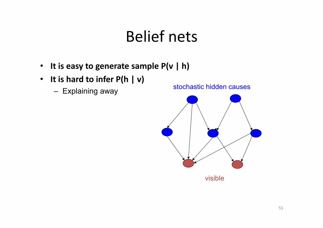
Belief nets
• It is easy to generate sample P(v | h)• It is hard to infer P(h | v)
– Explaining away
55
stochastic hidden causes
visible

Explaining away (Judea Pearl)• Even if two hidden causes are independent, they can become
dependent when we observe an effect that they can both influence. – If we learn that there was an earthquake it reduces the probability that the house jumped because of a truck.
truck hits house earthquake
house jumps
20 20
-20
-10 -10
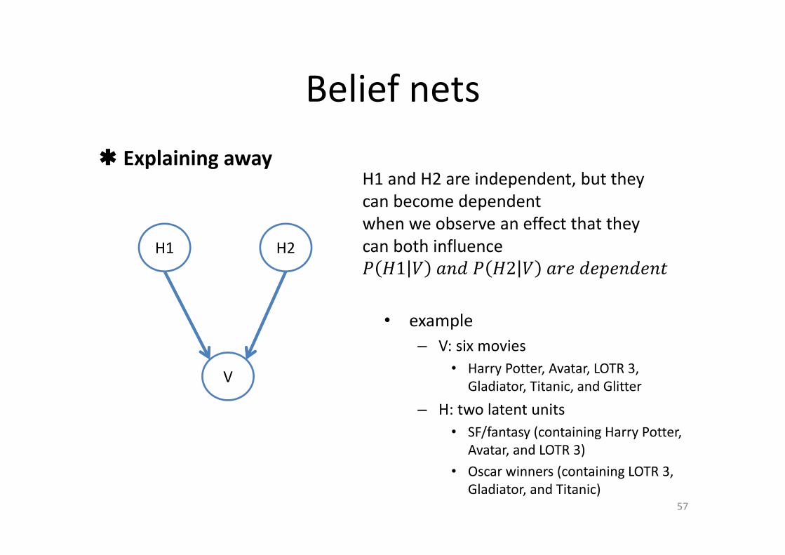
Belief nets Explaining away
57
H1 H2
V
H1 and H2 are independent, but they can become dependentwhen we observe an effect that they can both influence
1 2
• example– V: six movies
• Harry Potter, Avatar, LOTR 3, Gladiator, Titanic, and Glitter
– H: two latent units• SF/fantasy (containing Harry Potter,
Avatar, and LOTR 3) • Oscar winners (containing LOTR 3,
Gladiator, and Titanic)

Belief nets
• Some methods for learning deep belief nets– Monte Carlo methods
• But its painfully slow for large, deep belief nets
– Use Restricted Boltzmann Machines
58
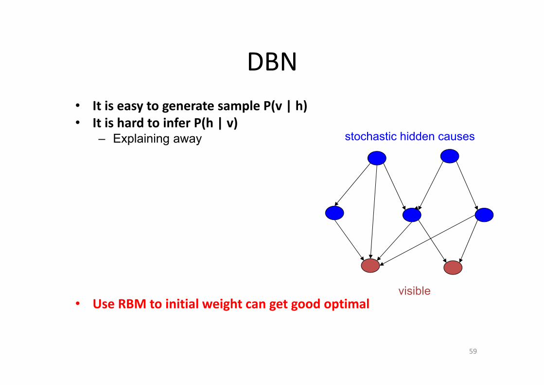
DBN• It is easy to generate sample P(v | h)• It is hard to infer P(h | v)
– Explaining away
• Use RBM to initial weight can get good optimal
59
stochastic hidden causes
visible

DBN
• Combining two RBMs to make a DBN
60
1W
2W2h
1h
1h
v
1W
2W
2h
1h
v
copy binary state for each v
Compose the two RBM models to make a single DBN model
Train this RBM first
Then train this RBM
It’s a deep belief nets!

DBN• Inference in a directed net with replicated
weights– Inference is trivial. We just multiply v0 by W transpose.– The model above h0 implements a complementary
prior.– Multiplying v0 by W transpose gives the
product of the likelihood term and the prior term.
– complementary priorsConsider observations x and hidden variables y, for a given likelihood function P(x|y), the priors of y, P(y) is called the complementary priors of P(x|y), provided that P(x,y)=P(x|y) P(y) leads to the posteriors P(y|x) that exactly factorises.
61
Wv1
h1
v0
h0
v2
h2
TW
TW
TW
W
W
etc.

DBN
• Complementary prior
• A Markov chain is a sequence of variables X1;X2; : : : with the Markov property
, … , |• A Markov chain is stationary if the transition probabilities do not
depend on time→
→ ′ is called the transition matrix.• If a Markov chain is ergodic it has a unique equilibrium distribution
→ → ∞
62
X1 X2 X3 X4

DBN• Most Markov chains used in practice satisfy detailed balance
→ ′ ′ ′ → e.g. Gibbs, Metropolis‐Hastings, slice sampling. . .
• Such Markov chains are reversible
63
X1 X2 X3 X4
→ → →
X1 X2 X3 X4
← ← ←
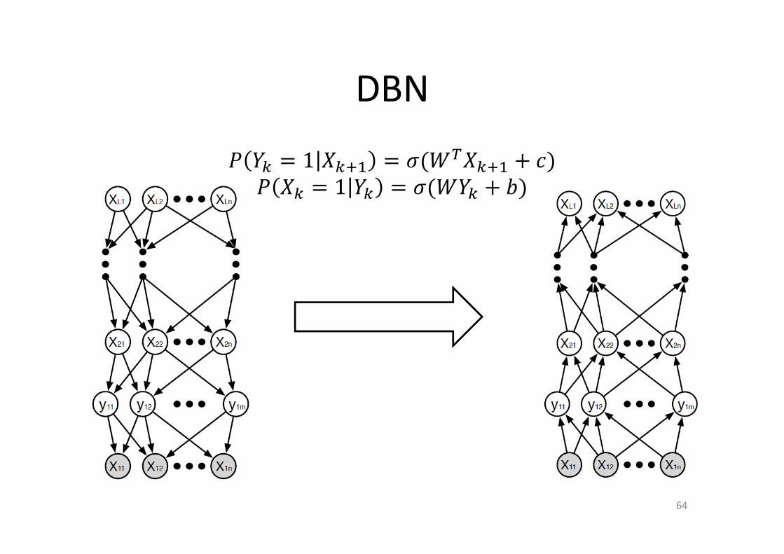
DBN
11
64

DBN
• Combining two RBMs to make a DBN
65
1W
2W2h
1h
1h
v
1W
2W
2h
1h
v
copy binary state for each v
Compose the two RBM models to make a single DBN model
Train this RBM first
Then train this RBM
It’s a deep belief nets!


• AutoEncoder• Restricted Boltzmann Machine (RBM)• Deep Belief Networks (DBN)• Convolutional Neural Networks (CNN)
Reference
• http://blog.echen.me/2011/07/18/introduction‐to‐restricted‐boltzmann‐machines/
• http://en.wikipedia.org/wiki/Restricted_Boltzmann_machine
• G . Hinton, Deep Belief Nets,2007 NIPS tutorial • https://class.coursera.org/neuralnets‐2012‐001/class/index
• http://en.wikipedia.org/wiki/Graphical_model• http://www.cs.toronto.edu/~hinton/csc2515/deeprefs.html

• Questions?