Deep Learning for Predicting Asset Returns

Guanhao Feng∗

College of Business

City University of Hong Kong

Jingyu He†

Booth School of Business

University of Chicago

Nicholas G. Polson ‡

Booth School of Business

University of Chicago

April 25, 2018

Abstract

Deep learning searches for nonlinear factors for predicting asset returns. Predictability is achieved

via multiple layers of composite factors as opposed to additive ones. Viewed in this way, asset

pricing studies can be revisited using multi-layer deep learners, such as rectified linear units

(ReLU) or long-short-term-memory (LSTM) for time-series effects. State-of-the-art algorithms

including stochastic gradient descent (SGD), TensorFlow and dropout design provide imple-

mentation and efficient factor exploration. To illustrate our methodology, we revisit the equity

market risk premium dataset of Welch and Goyal (2008). We find the existence of nonlinear

factors which explain predictability of returns, in particular at the extremes of the characteristic

space. Finally, we conclude with directions for future research.

Key Words: Deep Learning, Nonlinear Factor, Equity Premium, Empirical Asset Pricing, ReLU

Networks, LSTM

∗Address: 83 Tat Chee Avenue, Kowloon Tong, Hong Kong. E-mail address: gavin.feng@cityu.edu.hk.†Address: 5807 S Woodlawn Avenue, Chicago, IL 60637, USA. E-mail address: jingyu.he@chicagobooth.edu.‡Address: 5807 S Woodlawn Avenue, Chicago, IL 60637, USA. E-mail address: ngp@chicagobooth.edu.

1

arX

iv:1

804.

0931

4v2

[st

at.M

L]

26

Apr

201

8

1 Introduction

Deep learning searches for nonlinear factors to predict asset returns via a composition of factor-

based characteristics. Predicting asset returns is important to empirical finance and factor models

play a central role, for example, see Rosenberg et al. (1976) and Fama and French (1993). Cross-

sectional time series predictability is studied using predictive regressions, see Kandel and Stam-

baugh (1996), Barberis (2000) and Welch and Goyal (2008). We build on this line of research, by

incorporating deep learning with hierarchical layers of nonlinear factors to perform out-of-sample

prediction. Deep learning factors provide improvements at the extremes of the characteristic space

when explaining empirical asset returns. They provide an alternative to dynamic factor modeling,

see Lopes and Carvalho (2007), Carvalho et al. (2011) and Carvalho et al. (2017).

While the use of (artificial) neural networks is not novel in economics and finance, see Gal-

lant and White (1988a,b); Hornik et al. (1989); Gallant and White (1992); Kuan and White (1994);

Hutchinson et al. (1994); Lo (1994); Qi (1999); Jones (2006); Sirignano et al. (2016) and Heaton et al.

(2017), deep learning is new to characteristic-based asset pricing. Deep learning is capable of ex-

tracting nonlinear factors and provides a powerful alternative to feature selection and shrinkage

methods. Feng et al. (2017). Recent work of Kozak et al. (2017); Gu and Xiu (2018) shows the

promise of machine learning based predictors in empirical finance, including traditional regular-

ization methods and trees and. Feng et al. (2018) predicts cross-sectional returns with deep learn-

ing in a portfolio context. Deep networks, as opposed to shallow ones, can achieve out-of-sample

performance gains versus linear additive models, while avoiding the curse of dimensionality, for

example, see Poggio et al. (2017).

To predict the equity premium with a large set of economic variables, Welch and Goyal (2008)

leads to out-of-sample performance which is hard to outperform historical means. Improved method-

ologies have been suggested by Campbell and Thompson (2007), Rapach et al. (2010) and Harvey

et al. (2016) and, more recently, Feng et al. (2017) and Kozak et al. (2017). The latter relies on shrink-

ing the cross-sectional select which economic variables are of importance, rather than deep learning

which extracts nonlinear factors from the full characterisitc space with a goal of improved predictive

performance.

The rest of our paper is organized as follows. Section 1.1 discusses deep learning in financial

2

economics. Section 2 constructs our deep learning architectures for applications in forecasting the

equity premium. Section 3 shows simulation results. Section 4 reports our results on predicting

stock returns, mimicking the analysis of Welch and Goyal (2008). Finally, appendices contain details

on SGD and LSTM models as well as a comprehensive set of results on our empirical study.

1.1 Deep Learning Econometrics

Deep learning is a form of supervised learning for predicting an output variable, Y , via pre-

dictors, X . Deep learning comprises of a series of L non-linear transformations applied to the input

space X . Each of the L transformations is referred to as a layer, where the original input is X , the

output of the first transformation is the first layer, and so on, with the output Y as the (L + 1)-th

layer. We use l ∈ {1, . . . , L} to index the layers from 1 to L, which are called hidden layers. The

number of layers L represents the depth of the architecture.

Specifically, a deep neural network can be described as follows. Let f1, . . . , fL be given uni-

variate activation functions for each of the L layers. Activation functions are non-linear transforma-

tions of weighted data. Commonly used activation functions are sigmoidal (e.g., 1/(1 + exp(−x))

or tanh(x)), heaviside gate functions (e.g., I(x > 0)), or rectified linear units (ReLU) max{x, 0}. We

let Z(l) denote the l-th layer which is a vector with same length as number of neurons in that layer,

and so X = Z(0). The explicit structure of a deep prediction rule is then a composition of univariate

semi-affine functions,

FW,b = FW (1),b(1)

1 ◦ · · · ◦ FW (L),b(L)

L

FW (l),b(l)

l : = fl(W(l)Z(l) + b(l)) = fl

(Nl∑

i=1

W(l)i Z

(i)i + b

(l)i

), ∀1 ≤ l ≤ L

(1)

where Nl is the number of neurons or width of the architecture at layer l. W (l) are real weight ma-

trices and b(l) are threshold or activation level which contribute to the output of a hidden unit, al-

lowing the activation function to be shifted left or right. One noticeable property is that the weights

Wl ∈ RNl×Nl−1 are matrices. In an econometric perspective, deep learner models constitute a partic-

ular class of nonlinear neural network predictors. Fl denotes the l-th hidden layer. As in traditional

financial modeling we can view F (l) as latent factors. The main difference is that we will use a

3

composition of factors versus a traditional additive structure. Moreover, the hidden factors F (l) will

be extracted from the algorithm.

2 Deep Learning for Characteristic Based Asset Pricing

Let Rt+1 ∈ RT×1 be a vector of asset returns, Xt ∈ RT×p a high dimensional set of predictor

variables. Deep learning is a data reduction scheme that uses L layers of “hidden” factors, which

can be highly nonlinear. The factors are extracted from data set with the dual goal of good out-of-

sample prediction and in-sample model fit. Mean squared prediction error (MSPE) is a common

metric for out-of-sample predictor performance. From a finance viewpoint, we have a hierarchical

model of the formRt+1 = α+ βXt + βfFt + εt+1

Ft = FW,b(Xt)

FW,b : = fW1,b11 ◦ · · · ◦ fWL,bL

L

fWl,bl(Z) : = fl(WlZ + bl), ∀1 ≤ l ≤ L

(2)

where F : RT×p → RT×1 is a multivariate data reduction map represented as a deep learner. The

network parameters (W, b) are weights and offsets to be trained. Here εt are the usual idiosyncratic

pricing errors. The major difference between DL and traditional factor models are the useage of

compositions of factors rather shallow additive models. F is constructed as a composition of uni-

variate semi-affine functions and a common choice for activation function is fl(x) = max(x, 0) :=

ReLU(x), the so-called rectified linear unit. This leads to Deep ReLU networks which have been

popular in applications from image processing to game intelligence.

Traditionally, researchers estimate factors Ft and then learn coefficients α, β by regression with

a two-step procedure. Here Rt+1 is a linear additive combination of input variables Xt and latent

factors Ft,

Rt+1 = α+ βXt + βfFt

Deep learning will estimate coefficient α, β and latent factors, Ft, jointly. Figure 1 illustrates

this with green circles on left side as input predictors Xt for example, dividends, earnings, inflation

or other economic variables. The key advantage is non-linearity and simultaneous factor estima-

4

tion. The rightmost red circle is asset return Rt+1 to predict. The purple circles are fully connected

X1Dividends

X2Earnings

...

Book-to-Market

Inflation

X1

X2

f3

f4

f5

Hidden Layer1

Hidden Layer2

EconomicsVariables

ExcessReturn

Figure 1: Deep Learning architecture to estimate dynamic factor model

neurons in hidden layers. The yellow circles are the last hidden layer in equation 2, but are different

from the first hidden layer as they are composed of latent factors Ft generated by previous hidden

layers and a copy of the original input Xt.

To train a model, we need a loss function to minimize, which is typically mean squared error

of the in-sample fit of Rt+1.

L =1

T

T∑

t=1

(Rt+1 − Rt+1

)ᵀ(Rt+1 − Rt+1

)+ λφ

(β,W, b

), (3)

where φ(β,W, b

)is a regularization penalty to induce predictor selection and avoid model over-

fitting and λ controls the amount of regulations. The regressor parameters α, β, βf and factors Ft

jointly minimize loss function using stochastic gradient descent (SGD) algorithm in TensorFlow.

Another notable difference is that there is no stochastic error in the factor construction. Kandel

and Stambaugh (1996) discuss the difficulty of the model estimation and prediction in the presence

of parameter uncertainty. They propose a Bayesian framework to add a regularization prior on the

predictor existence and strength. Their model still cannot deal with an ultra high-dimensional xt as

5

well as its nonlinear signals.

3 Application

3.1 Simulation Study

To illustrate the possible gains available in deep learners for predictions, we provide a simula-

tion study to compare its prediction performance versus traditional machine learning tools such as

linear regression, Lasso, partial least squares and elastic net. As data generating processes, we use

one layer and two layers dynamic latent factor model.

Rt+1 = α+ βFt + εt+1

Ft = fl(WXt + b)

Similarly, the two layers data generating process is

Rt+1 = α+ βF2,t + εt+1

F1,t = fl(W(1)Xt + b(1))

F2,t = fl(W(2)F1,t + b(2))

The one hidden layer data generating process is described as follows. Suppose the length of

time series is T . Xt is a T × p matrix drawn from i.i.d. standard normal distribution. α, β, W and b

are coefficients also drawn from i.i.d. standard normal distribution. We control in-sample R2IS as a

measure of signal level, draw εt+1 from i.i.d. N(0, σ2) where σ2 are solved from equation

R2IS =

var(α+ βZt)

var(α+ βZt) + σ2.

where W (1), W (2), b(1), b(2) are coefficients drawn from i.i.d. standard normal. Xt is a T × p matrix

drawn from i.i.d. standard normal.

In the data generating process above, we generate R2 in the same way and regressors Xt,

output yt+1 and latent factors Ft. Three different deep learning architectures are compared: three

hidden layer deep learning model with 64 neurons in the first hidden layer, 32 neurons in the second

6

hidden layer and 16 neurons in the third hidden layer (DL-64-32-16). We add Xt to the last layer

(as shown in Figure 1), so there are actually p + 16 neurons in the third layer. Similarly we create

two hidden layer deep learning model with 32 and 16 neurons in each layer (DL-32-16) and one

16 neurons hidden layer model (DL-16). To illustrate the success of deep learning models, we also

compare with other frequently used approach such as ordinary least squares (OLS), partial least

squares (PLS), Lasso, elastic-net and “oracle OLS” which regress yt on latent factors Ft directly.

Oracle OLS is not possible to implement as we need to learn latent factors Ft from data. Shrinkage

parameters of Lasso and elastic net are selected by cross validation. For comparation, we use linear

regression, Lasso, Ridge, Elastic Net, PCA and PLS regressions. Simulation studies reveal that

neural network outperforms all other methods.

Table 1 provides results of one layer data generating process. Table 2 shows results of two

layers data generating process. It is straightforward to see that oracle OLS achieves smallest mean

squared prediction error (MSPE). The three deep learning models (DL 64-32-16, DL 32-16 and DL

16) are very similar to each other in all circumstances and all of them are much better than other

methods except oracle OLS as expected. Deep learning’s advantage over other approaches dimin-

ishes a little bit as R2 increases (noise level decreases). Table 1 shows the same pattern as Table 2,

our approach is the closest to oracle OLS.

K T R2MSPE

Oracle OLS PLS Lasso ElasNet DL 64-32-16 DL 32-16 DL 165 500 0.05 97.19 160.06 148.36 155.91 141.74 122.18 122.32 122.915 500 0.25 22.46 41.46 37.76 39.43 34.4 31.74 31.87 32.775 500 0.5 4.32 9.42 8.53 8.65 7.5 7.4 7.33 7.785 500 0.75 1.93 6.25 5.74 5.82 5.31 5.17 5.17 5.47

25 500 0.05 588.16 874.51 800.94 864.13 813.82 665.27 660.89 650.7125 500 0.25 93.49 159.21 145.91 154.74 140.71 123.59 123.49 123.6325 500 0.5 22.56 44.51 40.94 42.75 38.42 35.43 35.27 36.1525 500 0.75 12.85 36.41 32.42 34.9 31.58 29.61 29.48 30.54

Table 1: One layer data generating process. P is dimension of Xt, K is dimension of latent factorsZt, T is length of time series. KPLS is number of factors used in principal regression. R2 is Rsquared of DGP, Rt+1 = α+ βFt + εt+1. The oracle regresses Rt on Ft, all other methods regress Rt

on xt. Dropout = 0.5

7

P K1 K2 T R2MSPE

Oracle OLS PLS Lasso Elastic-Net DL 64-32-16100 25 25 500 0.05 1130.05 1401.06 1302.05 1390.49 1329.43 1088.67100 25 25 500 0.25 121.57 160.04 143.22 155.72 140.31 117.92100 25 25 500 0.5 22.74 38.48 35.98 37.19 34.04 32.17100 25 25 500 0.75 8.61 19.57 17.64 18.67 16.95 15.62100 25 5 500 0.05 146.81 244.75 223.29 239.48 219.26 183.25100 25 5 500 0.25 15.35 30.62 27.58 28.94 24.75 21.61100 25 5 500 0.5 4.19 9.25 8.50 8.65 7.61 7.03100 25 5 500 0.75 1.14 3.85 3.54 3.50 3.18 3.01

Table 2: Two layers data generating process. P is dimension of Xt, K1 and K2 are dimensions oflatent factors Z1

t and Z2t respectively. T is length of time series. KPLS is number of factors used in

principal regression. R2 is R squared of DGP, Rt+1 = α + βFt + εt+1. Oracle regresses Rt on Ft, allother methods regress Rt on xt.

4 Predict Asset Returns

Data. Predicting market excess returns is a challenge as usually predictors have difficulty in outper-

forming historical mean averages. Welch and Goyal (2008) explore the out-of-sample excess market

return predictability of S&P 500 based on a large set of economic predictor variables.

Table 3 provides the variable descriptions. The sample frequency is monthly data, beginning

in 1926 December to 2016 December, giving 90 years in total.

Variable Descriptiond/p dividend price ratiod/y dividend yield ratioe/p earning price ratiod/e dividend payout ratiosvar stock varianceb/m book to market rationtis net issuestbl treasury bills rateltr long term rate

tms term spreaddfy default spreaddfr default return spreadinfl consumer price indexcay consumption, wealth, income ratio

Table 3: Description of all variables

8

Predictive Regressions. A predictive regression model takes the form

Rt+1 = α+ βᵀXt + εt+1

Xt = A+BXt−1 + ut.

Here, Rt+1 is the logarithm return on a market portfolio S&P 500. Xt is a p × 1 predictor from the

lag period and follows a VAR(1) model.

Our deep learning dynamic factor model builds on this by assuming

Rt+1 = α+ βXt + βfFt + εt+1

Ft = FW,b(Xt)

Deep learning structures are flexible enough that we need to specify number of hidden layers and

number of neurons in each layer. We present result of a variety of deep learning structures (DL1 to

DL4) and compare with a range of frequently used methods such as ordinary least squares (OLS),

ridge regression (Ridge), partial least squares (PLS), Lasso and elastic-net. For example, for model

DL1, 32-16-8 means a three layers deep network with 32, 16 and 8 neurons in the three hidden layers

respectively. The shrinkage level is a critical tuning parameter for Lasso and elastic net, which is

selected by cross validation.

Method DescriptionDL1 32-16-8DL2 16-8-4DL3 16-8DL4 16OLS ordinary least squares

Ridge ridge regressionPLS partial least squares

Lasso LassoElasNet elastic net

Table 4: Description of all methods for comparision

Input variables. We consider four different cases of input variables with growing dimensionality.

In the first case, the input variables are the original 14 variables Xt as shown in table 3. The second

case has squared terms (Xt, X2t ) and 28 variables in total. In the third case we add an asymmetric

9

term (Xt, I{Rt−1 > 0} × Xt) where I{Rt−1 > 0} is an indicator whether the return of previous

period is positive or not. In the last case, we use all variables above as (Xt, X2t , I{Rt−1 > 0} ×Xt),

42 variables in total.

Output variables. We predict the excess logarithm return of S&P 500, which is the difference be-

tween logarithm return of S&P 500 and risk-free interest rate. Welch and Goyal (2008) points out

that although it is not clear how to choose the periods over which a regression model is estimated

and subsequently evaluated, it is important to have enough initial data to get a reliable regression

estimate at the start of the evaluation period. We predict three kinds of returns: one, three and

twelve months returns.

Training set specifications. We also explore two period specifications. The first one uses a fixed

(50 years) moving window to estimate the model and predicts the following period. The second

one uses a cumulative moving window which starts from 1926 December to the current month and

predicts the next period. Therefore the second specification uses more and more data as the window

moving with time.

Forecast Evaluations. To compare prediction results Rt+1 and Rt+1, we use out-of-sample R2OS as

suggested by Campbell and Thompson (2007). The R2OS statistics is akin to in-sample R2 and is

defined by

R2OS = 1−

∑Pk=P0+1(Rt+k − Rt+k)2

∑Pt=P0+1(Rt+k − Rt+k)2

. (4)

where Rt+k is the prediction of a predictive model. Rt+k is forecast of historical mean. When

R2OS > 0, the predictive regression model has better mean squared prediction error (MSPE) than

the benchmark average historical return. The most popular method for testing significant differ-

ence in MSPE is the Diebold and Mariano (2002) and West (1996) test. Even if there is evidence

that R2OS is statistically significant, R2

OS values are typically small for prediction models, but as

Campbell and Thompson (2007) and Rapach et al. (2010) argue, even very small the R2OS values

can be economically meaningful in terms of portfolio returns. We find the same is true for our non-

linear deep learning prediction rules. Figure 2 shows histogram of R2OS for all methods and more

comprehensive tables are provided in the appendix.

10

Empirical Results. Figure 2 shows MSPE and R2 of 1-month predictions for moving window and

cumulative windows. Comprehensive tables can be found in the appendix. Here we summarize the

broad trends that merges. All other methods get negativeR2OS , which is consistent with conclusions

of Welch and Goyal (2008) that all predictive regression models cannot beat simple historical mean.

However, most deep learning approaches get slightly positive R2OS in all four different input cases,

which indicates that they have a smaller mean squared error than historical mean. The results of

predicting one month return using cumulative width moving window are shown in table 6, where

deep learning methods achieve higher R2OS than fixed width 600-month moving window because

deep learning model can learn the nonlinear structures better with more training observations. Note

that OLS has much lower negative R2OS in table 6 because it cannot learn the complex trend well in

a longer time horizon.

Figure 3 shows fitted latent factor of DL1 (32-16-8) model. We plot the 8 latent factors against

the first 4 input variables d/p, d/y, e/p and d/e. It straightforward to see that deep learning model

learns highly nonlinear factors from the data.

−0.2

−0.1

0.0

DL1 DL2 DL3 DL4 ElasticNet Lasso OLS PLS Ridge

Method

R2

Input

Case 1

Case 2

Case 3

Case 4

(a) R2 of 1 month return predictions. Mov-ing window.

−12.5

−10.0

−7.5

−5.0

−2.5

0.0

DL1 DL2 DL3 DL4 ElasticNet Lasso OLS PLS Ridge

Method

R2

Input

Case 1

Case 2

Case 3

Case 4

(b) R2 of 1 month return predictions. Cu-mulative window.

Figure 2: We generate 8 latent factors by fitting a three layer deep dynamic factor model with 32, 16and 8 neurons in each layer. The plot shows the latent factors against first 4 variables d/p, d/y, e/pand d/e. Strong non-linearity exists.

11

3.6 3.4 3.2 3.0 2.8dp, dividend price ratio

0.00

0.05

0.10

0.15

0.20

0.25

0.30

0.35

Late

nt fa

ctor

s

(a) d/p, dividend price ratio

3.6 3.4 3.2 3.0 2.8dy, dividend yield ratio

0.00

0.05

0.10

0.15

0.20

0.25

0.30

0.35

Late

nt fa

ctor

s

(b) d/y, dividend yield ratio

3.2 3.0 2.8 2.6 2.4 2.2 2.0ep, earning price ratio

0.00

0.05

0.10

0.15

0.20

0.25

0.30

0.35

Late

nt fa

ctor

s

(c) e/p, earning price ratio

1.0 0.9 0.8 0.7 0.6 0.5 0.4 0.3de, dividend payout ratio

0.00

0.05

0.10

0.15

0.20

0.25

0.30

0.35

Late

nt fa

ctor

s

(d) d/e, dividend payout ratio

Figure 3: We generate 8 latent factors by fitting a three layer deep dynamic factor model with 32, 16and 8 neurons in each layer, using input variables in case 1. The plot shows 8 latent factors againstfirst 4 variables d/p, d/y, e/p and d/e. Each color indicates one latent factor.

Comparison with Trees. We do further analysis to show the difference between deep learning and

tree based methods. Instead of prediction the logarithm return of S&P 500, we predict whether the

market crash or not, where the definition of a crash is that monthly return is worse than −10%.

Therefore, the regression problem is converted to a classification problem.

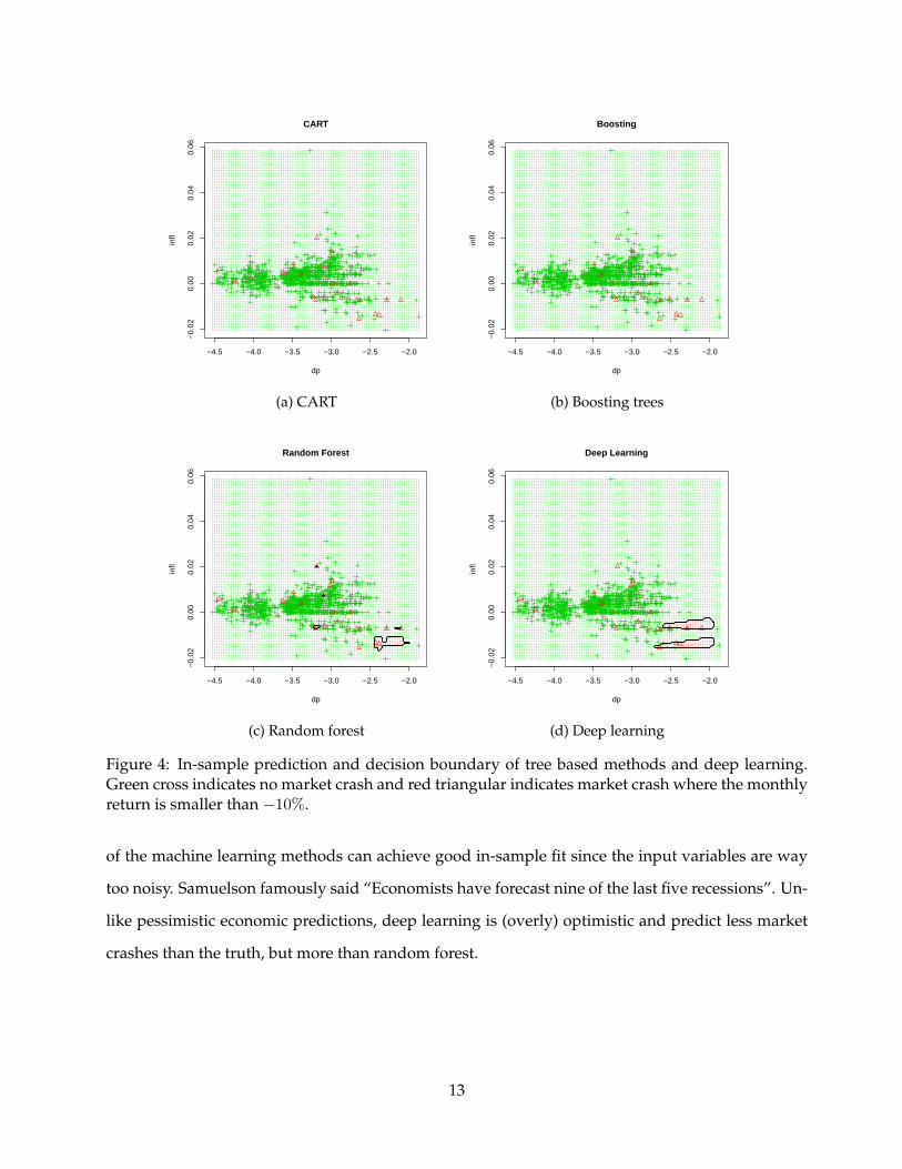
Figure 4 shows the in-sample fit of deep learning and tree based methods using two economic

variables dividend price ratio (dp) and inflation (infl). It’s straightforward to see that Both CART

and boosting always predict “no crash” no matter what value the input variables take. Deep learn-

ing does slightly better than random forest because it captures more tail behavior. However, none

12

−4.5 −4.0 −3.5 −3.0 −2.5 −2.0

−0.

020.

000.

020.

040.

06

CART

dp

infl

(a) CART

−4.5 −4.0 −3.5 −3.0 −2.5 −2.0

−0.

020.

000.

020.

040.

06

Boosting

dp

infl

(b) Boosting trees

−4.5 −4.0 −3.5 −3.0 −2.5 −2.0

−0.

020.

000.

020.

040.

06

Random Forest

dp

infl

(c) Random forest

−4.5 −4.0 −3.5 −3.0 −2.5 −2.0

−0.

020.

000.

020.

040.

06

Deep Learning

dp

infl

(d) Deep learning

Figure 4: In-sample prediction and decision boundary of tree based methods and deep learning.Green cross indicates no market crash and red triangular indicates market crash where the monthlyreturn is smaller than −10%.

of the machine learning methods can achieve good in-sample fit since the input variables are way

too noisy. Samuelson famously said “Economists have forecast nine of the last five recessions”. Un-

like pessimistic economic predictions, deep learning is (overly) optimistic and predict less market

crashes than the truth, but more than random forest.

13

5 Discussion

Deep learning dynamic factor models are constructed for predicting asset returns. Both hid-

den factors and regression coefficients are jointly estimated by stochastic gradient descent. Deep

learning is a very flexible class of machine learning tools for empirical analysis. By varying the

number of hidden layers and the number of neurons within each layer, very flexible predictors can

be training, and out-of-sample cross-validation provides a technique to avoid overfitting. Long-

short-term-memory (LSTM) models are alternatives to traditional state space modeling.

Deep learning methods have some advantages and caveats. The key advantages are: (i) With

TensorFlow, it is easy to implement deep learning architectures, (ii) Composite versus additive

models, (iii) Hyperplanes versus cylinder sets. With the coefficient term W , deep learning model

can rotate input variables and create cutoff hyperplanes. Hence better classification rules, (iv) Able

to fit in-sample far more accurately.

The key caveats are (i) Model interpretability, (ii) Learn only correlation but not causation, (iii)

Despite many gains from neural networks to detect and exploit interactions in empirical that are

hard to identify using existing economic theory, they have several important limitations. In partic-

ular, perform causal inference from large datasets is hard when there are complex data interactions

without taking assumptions for economic model specification. Due to the nesting of layers, statisti-

cal inference cannot always be applied to deep learning. Yet, deep learning provides a very fruitful

linear of research particularly in empirical asset pricing studies.

14

References

Barberis, N. (2000). Investing for the long run when returns are predictable. The Journal of Fi-

nance 55(1), 225–264.

Campbell, J. Y. and S. B. Thompson (2007). Predicting excess stock returns out of sample: Can

anything beat the historical average? The Review of Financial Studies 21(4), 1509–1531.

Carvalho, C. M., H. F. Lopes, and O. Aguilar (2011). Dynamic stock selection strategies: A structured

factor model framework. Bayesian Statistics 9, 1–21.

Carvalho, C. M., H. F. Lopes, and R. E. McCulloch (2017). On the long run volatility of stocks.

Journal of the American Statistical Association.

Cho, K., B. Van Merrienboer, D. Bahdanau, and Y. Bengio (2014). On the properties of neural ma-

chine translation: Encoder-decoder approaches. arXiv:1409.1259.

Dean, J., G. Corrado, R. Monga, K. Chen, M. Devin, M. Mao, A. Senior, P. Tucker, K. Yang, Q. V.

Le, et al. (2012). Large scale distributed deep networks. Advances in Neural Information Processing

Systems, 1223–1231.

Diebold, F. X. and R. S. Mariano (2002). Comparing predictive accuracy. Journal of Business &

Economic Statistics 20(1), 134–144.

Fama, E. F. and K. R. French (1993). Common risk factors in the returns on stocks and bonds. Journal

of Financial Economics 33(1), 3–56.

Feng, G., S. Giglio, and D. Xiu (2017). Taming the factor zoo. https://ssrn.com/abstract=2934020.

Feng, G., N. G. Polson, and J. Xu (2018). Deep Learning Alpha. Technical report, The University of

Chicago.

Gallant, A. R. and H. White (1988a). There exists a neural network that does not make avoidable

mistakes. In Proceedings of the Second Annual IEEE Conference on Neural Networks, San Diego, CA, I.

Gallant, A. R. and H. White (1988b). A unified theory of estimation and inference for nonlinear dynamic

models. Blackwell.

15

Gallant, A. R. and H. White (1992). On learning the derivatives of an unknown mapping with

multilayer feedforward networks. Neural Networks 5(1), 129–138.

Gu, Shihao, K. B. and D. Xiu (2018). Empirical asset pricing via machine learning.

https://ssrn.com/abstract=3159577.

Harvey, C. R., Y. Liu, and H. Zhu (2016). And the cross-section of expected returns. The Review of

Financial Studies 29(1), 5–68.

Heaton, J., N. Polson, and J. H. Witte (2017). Deep learning for finance: deep portfolios. Applied

Stochastic Models in Business and Industry 33(1), 3–12.

Hinton, G. E. and R. R. Salakhutdinov (2006). Reducing the dimensionality of data with neural

networks. Science 313(5786), 504–507.

Hochreiter, S. and J. Schmidhuber (1997). Long Short-Term Memory. Neural Computation 9(8), 1735–

1780.

Hornik, K., M. Stinchcombe, and H. White (1989). Multilayer feedforward networks are universal

approximators. Neural Networks 2(5), 359–366.

Hutchinson, J. M., A. W. Lo, and T. Poggio (1994). A nonparametric approach to pricing and hedging

derivative securities via learning networks. The Journal of Finance 49(3), 851–889.

Jones, C. S. (2006). A nonlinear factor analysis of S&P 500 index option returns. The Journal of

Finance 61(5), 2325–2363.

Kandel, S. and R. F. Stambaugh (1996). On the predictability of stock returns: an asset-allocation

perspective. The Journal of Finance 51(2), 385–424.

Kozak, S., S. Nagel, and S. Santosh (2017). Shrinking the cross section. Technical report, National

Bureau of Economic Research.

Kuan, C.-M. and H. White (1994). Artificial neural networks: an econometric perspective. Econo-

metric Reviews 13(1), 1–91.

16

Lake, B. M., R. Salakhutdinov, and J. B. Tenenbaum (2015). Human-level concept learning through

probabilistic program induction. Science 350(6266), 1332–1338.

Lo, A. W. (1994). Neural networks and other nonparametric techniques in economics and finance.

In AIMR Conference Proceedings, Number 9. CFA Institute.

Lopes, H. F. and C. M. Carvalho (2007). Factor stochastic volatility with time varying loadings and

markov switching regimes. Journal of Statistical Planning and Inference 137(10), 3082–3091.

Poggio, T., H. Mhaskar, L. Rosasco, B. Miranda, and Q. Liao (2017). Why and when can deep-but not

shallow-networks avoid the curse of dimensionality: A review. International Journal of Automation

and Computing 14(5), 503–519.

Qi, M. (1999). Nonlinear predictability of stock returns using financial and economic variables.

Journal of Business & Economic Statistics 17(4), 419–429.

Rapach, D. E., J. K. Strauss, and G. Zhou (2010). Out-of-sample equity premium prediction: Com-

bination forecasts and links to the real economy. The Review of Financial Studies 23(2), 821–862.

Rosenberg, B., V. Marathe, et al. (1976). Common factors in security returns: Microeconomic deter-

minants and macroeconomic correlates. Technical report, University of California at Berkeley.

Sirignano, J., A. Sadhwani, and K. Giesecke (2016). Deep learning for mortgage risk.

arXiv:1607.02470.

Srivastava, N., G. Hinton, A. Krizhevsky, I. Sutskever, and R. Salakhutdinov (2014). Dropout: A

simple way to prevent neural networks from overfitting. The Journal of Machine Learning Re-

search 15(1), 1929–1958.

Welch, I. and A. Goyal (2008). A comprehensive look at the empirical performance of equity pre-

mium prediction. Review of Financial Studies 21(4), 1455–1508.

West, K. D. (1996). Asymptotic inference about predictive ability. Econometrica: Journal of the Econo-

metric Society, 1067–1084.

17

A Complete Results of Predicting Asset Returns

A.1 1 month return prediction

Case 1 Case 2 Case 3 Case 4

MSPE R2OS MSPE R2

OS MSPE R2OS MSPE R2

OS

OLS 0.00224 -0.15680 0.00235 -0.21513 0.00218 -0.12647 0.00242 -0.27127Ridge 0.00201 -0.03761 0.00202 -0.04316 0.00205 -0.05721 0.00202 -0.06075PLS 0.00223 -0.15022 0.00233 -0.20209 0.00216 -0.11637 0.00240 -0.25753Lasso 0.00193 0.00165 0.00193 0.00322 0.00193 0.00138 0.00191 -0.00164ElasticNet 0.00193 0.00145 0.00193 0.00313 0.00193 0.00133 0.00191 -0.00157DL1 0.00192 0.01864 0.00192 0.00695 0.00193 0.00517 0.00189 0.00665DL2 0.00192 0.00784 0.00193 0.00441 0.00192 0.01111 0.00189 0.00766DL3 0.00192 0.00941 0.00192 0.00885 0.00192 0.00851 0.00189 0.00761DL4 0.00195 0.01103 0.00194 -0.00355 0.00195 -0.00654 0.00193 -0.01471

Table 5: Prediction 1 month logarithm return of S&P 500. The training data is a fixed length 600month moving window.

Case 1 Case 2 Case 3 Case 4

MSPE R2OS MSPE R2

OS MSPE R2OS MSPE R2

OS

OLS 0.01346 -6.43907 0.01487 -7.22048 0.01589 -7.74735 0.02347 -11.91466Ridge 0.00263 -0.45303 0.00242 -0.33556 0.00313 -0.72119 0.00288 -0.58245PLS 0.01355 -6.48721 0.01283 -6.08951 0.01729 -8.51291 0.01848 -9.16937Lasso 0.00199 -0.09974 0.00182 -0.00534 0.00204 -0.12395 0.00181 0.00629ElasticNet 0.00200 -0.10585 0.00182 -0.00330 0.00204 -0.12382 0.00181 0.00477DL1 0.00179 0.01348 0.00178 0.01390 0.00178 0.01867 0.00178 0.01864DL2 0.00178 0.01376 0.00178 0.01433 0.00178 0.01922 0.00178 0.01850DL3 0.00179 0.01318 0.00179 0.01280 0.00179 0.01710 0.00178 0.01792DL4 0.00186 -0.02858 0.00187 -0.03178 0.00191 -0.05172 0.00189 -0.03882

Table 6: Prediction 1 month logarithm return of S&P 500. The training data is a cumulative window.

18

A.2 3 month return prediction

Case 1 Case 2 Case 3 Case 4

MSPE R2OS MSPE R2

OS MSPE R2OS MSPE R2

OS

OLS 0.00767 -0.27961 0.00839 -0.39954 0.00802 -0.33652 0.00871 -0.44996Ridge 0.00670 -0.11741 0.00679 -0.13296 0.00693 -0.15497 0.00694 -0.15661PLS 0.00762 -0.27214 0.00821 -0.37061 0.00795 -0.32459 0.00836 -0.39237Lasso 0.00602 -0.00373 0.00602 -0.00457 0.00605 -0.00696 0.00604 -0.00648ElasticNet 0.00602 -0.00513 0.00602 -0.00455 0.00605 -0.00692 0.00604 -0.00659DL1 0.00593 0.01045 0.00594 0.00927 0.00595 0.00915 0.00595 0.00937DL2 0.00593 0.01023 0.00593 0.01099 0.00595 0.00970 0.00593 0.01266DL3 0.00593 0.01074 0.00593 0.01042 0.00593 0.01233 0.00595 0.00911DL4 0.00600 -0.00084 0.00600 -0.00041 0.00607 -0.01173 0.00595 0.00889

Table 7: Prediction 3 month logarithm return of S&P 500. The training data is a fixed length 600month moving window.

Case 1 Case 2 Case 3 Case 4

MSPE R2OS MSPE R2

OS MSPE R2OS MSPE R2

OS

OLS 0.06657 -10.09405 0.08616 -13.35903 0.05972 -8.96527 0.10663 -16.79488Ridge 0.01306 -1.17639 0.01444 -1.40593 0.01343 -1.24067 0.01482 -1.47293PLS 0.06816 -10.35922 0.09308 -14.51277 0.08010 -12.36732 0.09960 -15.62057Lasso 0.00798 -0.32950 0.00756 -0.26015 0.00719 -0.19937 0.00714 -0.19080ElasticNet 0.00797 -0.32892 0.00762 -0.27018 0.00729 -0.21706 0.00735 -0.22640DL1 0.00571 0.04783 0.00571 0.04767 0.00571 0.04737 0.00571 0.04680DL2 0.00571 0.04760 0.00571 0.04759 0.00570 0.04799 0.00570 0.04799DL3 0.00572 0.04680 0.00572 0.04678 0.00571 0.04655 0.00571 0.04647DL4 0.00602 -0.00360 0.00603 -0.00409 0.00623 -0.03891 0.00618 -0.03126

Table 8: Prediction 3 month logarithm return of S&P 500. The training data is a cumulative window.

19

A.3 12 month return prediction

Case 1 Case 2 Case 3 Case 4

MSPE R2OS MSPE R2

OS MSPE R2OS MSPE R2

OS

OLS 0.02903 -0.12388 0.03320 -0.28541 0.03308 -0.28480 0.03700 -0.43717Ridge 0.02788 -0.07920 0.02864 -0.10883 0.02917 -0.13287 0.02991 -0.16163PLS 0.02894 -0.12034 0.03233 -0.25154 0.03018 -0.17200 0.03322 -0.29019Lasso 0.02703 -0.04662 0.02700 -0.04529 0.02709 -0.05211 0.02706 -0.05107ElasticNet 0.02714 -0.05069 0.02711 -0.04954 0.02713 -0.05371 0.02718 -0.05553DL1 0.02496 0.03361 0.02497 0.03324 0.02504 0.02756 0.02502 0.02824DL2 0.02494 0.03450 0.02496 0.03356 0.02499 0.02948 0.02496 0.03060DL3 0.02499 0.03268 0.02499 0.03272 0.02516 0.02296 0.02505 0.02729DL4 0.02607 -0.00936 0.02584 -0.00041 0.02664 -0.03445 0.02628 -0.02076

Table 9: Prediction 12 month logarithm return of S&P 500. The training data is a fixed length 600month moving window.

Case 1 Case 2 Case 3 Case 4

MSPE R2OS MSPE R2

OS MSPE R2OS MSPE R2

OS

OLS 0.47498 -14.73602 0.51265 -15.98412 0.65768 -21.26662 0.69387 -22.49201Ridge 0.09795 -2.24502 0.10592 -2.50926 0.10892 -2.68761 0.11665 -2.94934PLS 0.46656 -14.45711 0.47528 -14.74595 0.56927 -18.27361 0.56701 -18.19688Lasso 0.04705 -0.55869 0.04714 -0.56159 0.04596 -0.55601 0.04433 -0.50088ElasticNet 0.04634 -0.53519 0.04605 -0.52564 0.04480 -0.51667 0.04258 -0.44144DL1 0.02619 0.13242 0.02608 0.13601 0.02625 0.11129 0.02611 0.11611DL2 0.02617 0.13290 0.02611 0.13505 0.02618 0.11352 0.02614 0.11492DL3 0.02624 0.13071 0.02605 0.13687 0.02634 0.10838 0.02614 0.11493DL4 0.03016 0.00069 0.03019 -0.00017 0.03355 -0.13583 0.03240 -0.09704

Table 10: Prediction 12 month logarithm return of S&P 500. The training data is a cumulativewindow.

20

B Dropout

Dropout Hinton and Salakhutdinov (2006) and Srivastava et al. (2014) is a technique designed

to avoid over-fitting in the training process. Input dimensions in X are removed randomly with

a given probability p. This affects the underlying loss function and optimization problem. For

example, if L(Y, Y ) = ‖Y − Y ‖22, where Y = WX . When marginalizing over the randomness, we

have a new objective

arg minW ED∼Ber(p)‖Y −W (D ?X)‖22 ,

which is equivalent to

arg minW ‖Y − pWX‖22 + p(1− p)‖(diag(X>X))12W‖22 ,

which is ridge a penalty under a g-prior. The dropout architecture is

Y(l)i = D(l) ? X(l), where D(l) = (D

(l)1 , · · · , D(l)

p ) ∼ Ber(p)

Y(l)i = f(W

(l)i X(l) + b

(l)i )

where in effect, the input X is replaced by D ?X , where ? denotes the element-wise product and D

is a matrix of independent Bernoulli Ber(p) distributed random variables.

21

C Deep Long-Short-Term-Memory

Traditional recurrent neural nets (RNNs) can learn complex temporal dynamics via the set of

deep recurrence equations

Zt = f(WxzXt +Wzz + bx),

Yt = f(WhzZt + bz),

where Yt is the output at time t, Xt is the input, Zt is the hidden layer with N hidden units. For

length T the updates are computed sequentially.

Long-short-term-memories (LSTMs) are a particular form of recurrent network which provide

a solution by incorporating memory units, see Hochreiter and Schmidhuber (1997). This allows

the network to learn when to forget previous hidden states and when to update hidden states given

new information. Models with hidden units with varying connections within the memory unit have

been proposed in the literature with great empirical success. Specifically, in addition to a hidden

unit, LSTMs include an input gate, a forget gate, an input modulation gate, and a memory cell.

The memory cell unit combines the previous memory cell unit which is modulated by the forget

and input modulation gate together with the previous hidden state, modulated by the input gate.

These additional cells enable an LSTM architecture to learn extremely complex long-term temporal

dynamics that a vanilla RNN is not capable of. Additional depth can be added to LSTMs by stacking

them on top of each other, using the hidden state of the LSTM as the input to the next layer.

State ht = σ(ot)� tanh(ct)

Equations ct = σ(ft)� ct−1 + σ(it)� tanh(kt)

it

kt

ft

ot

=

Wix Wih

Wkx Wkh

Wfx Wfh

Wox Woh

xt

ht−1

+

bi

bk

bf

bo

(5)

where � denotes element-wise vector product. The term σ(ft) � ct−1 introduces the long-range

22

dependence. kt is new information flow to the current cell. The states (ft, it) controls weights of

past memory and new information. ft is also called forget gate. The parameters (W, b) of the stacked

weight and bias vectors are learned by stochastic gradient descend (SGD) in TensorFlow. LSTM

cell is defined by a state equation which is updated deterministically as

ht

ct

= LSTMCell(yt, ht−1) (6)

Figure 5: Structure of an LSTM cell

Figure 5 demonstrates the architecture of one LSTM cell. Let yt denote the observed time series

and ht a hidden state. ct is the “memory” pass through multiple LSTM cells. The hidden state ht is

generated using another hidden cell state, ct that will be generated so long term dependencies are

allowed to flow in the network. The output state, ht is generated by a sequence of transformations

known as an LSTMCell operator.

The key addition, compared to an RNN, is the hidden state ct, the information is added or

removed from the memory state via layers defined via a sigmoid function σ(x) = (1 + e−x)−1 and

point-wise multiplication ⊗. The first gate ft ⊗ ct−1, called the forget gate, allows to throw away

some data from the previous cell state. The next gate, it ⊗ kt, called the input gate, decides which

values will be updated. Then the new cell state is a sum of the previous cell state, passed through the

forgot gate selected components. This provides a mechanism for dropping irrelevant information

from the past and adding relevant information from the current time step. Finally, the output layer,

ot ⊗ tanh(ct), returns tanh applied to the hidden state with some of the entries removed.

23