Journal Pre-proof

Deep-learning-based surrogate model for reservoir simulation withtime-varying well controls

Zhaoyang Larry Jin, Yimin Liu, Louis J. Durlofsky

PII: S0920-4105(20)30353-3DOI: https://doi.org/10.1016/j.petrol.2020.107273Reference: PETROL 107273

To appear in: Journal of Petroleum Science and Engineering

Received date : 11 November 2019Revised date : 15 March 2020Accepted date : 5 April 2020

Please cite this article as: Z.L. Jin, Y. Liu and L.J. Durlofsky, Deep-learning-based surrogate modelfor reservoir simulation with time-varying well controls. Journal of Petroleum Science andEngineering (2020), doi: https://doi.org/10.1016/j.petrol.2020.107273.

This is a PDF file of an article that has undergone enhancements after acceptance, such as theaddition of a cover page and metadata, and formatting for readability, but it is not yet the definitiveversion of record. This version will undergo additional copyediting, typesetting and review before itis published in its final form, but we are providing this version to give early visibility of the article.Please note that, during the production process, errors may be discovered which could affect thecontent, and all legal disclaimers that apply to the journal pertain.

© 2020 Published by Elsevier B.V.

1

2

3

4

5

6

7

8

9

10

11

12

13

14

15

16

17

18

19

20

21

22

23

24

25

26

27

28

29

30

31

32

33

34

35

36

37

38

39

40

41

42

43

44

45

46

47

48

49

50

51

52

53

54

55

56

57

58

59

60

61

62

63

64

65

Deep-learning-based surrogate model for reservoir simulation with

time-varying well controls

Zhaoyang Larry Jina,∗, Yimin Liua, Louis J. Durlofskya

aDepartment of Energy Resources Engineering, Stanford University, Stanford, CA, 94305

Abstract

A new deep-learning-based reduced-order modeling (ROM) framework is proposed forapplication in subsurface flow simulation. The reduced-order model is based on an exist-ing embed-to-control (E2C) framework and includes an auto-encoder, which projects thesystem to a low-dimensional subspace, and a linear transition model, which approximatesthe evolution of the system states in low dimension. In addition to the loss function fordata mismatch considered in the original E2C framework, we introduce a physics-based lossfunction that penalizes predictions that are inconsistent with the governing flow equations.The loss function is also modified to emphasize accuracy in key well quantities of inter-est (e.g., fluid production rates). The E2C ROM is shown to be analogous to an existingROM, POD-TPWL, which has been extensively developed for subsurface flow simulation.The new ROM is applied to oil-water flow in a heterogeneous reservoir, with flow driven bynine wells operating under time-varying control specifications. A total of 300 high-fidelitytraining simulations are performed in the offline stage, and the network training requires 10-12 minutes on a Tesla V100 GPU node. Online (runtime) computations achieve speedups ofover a factor of 1000 relative to full-order simulations. Extensive test case results, with wellcontrols varied over large ranges, are presented. Accurate ROM predictions are achieved forglobal saturation and pressure fields at particular times, and for injection and productionwell responses as a function of time. Error is shown to increase when 100 or 200 (rather than300) training runs are used to construct the E2C ROM. Overall the E2C ROM is shown toprovide reliable predictions with levels of perturbations in the well controls that are muchlarger than those used with existing POD-TPWL treatments. The current model is howeverlimited to 2D systems, and the required number of training simulations is much larger thanthat for POD-based ROMs.

Keywords: reservoir simulation, reduced-order model, deep learning, physics-informedneural network, auto-encoder, embed-to-control, E2C

∗Corresponding authorEmail addresses: zjin@stanford.edu (Zhaoyang Larry Jin), yiminliu@stanford.edu (Yimin Liu),

lou@stanford.edu (Louis J. Durlofsky)

Preprint submitted to Journal of Petroleum Science and Engineering March 15, 2020

*Revised manuscript with changes marked

Jour

nal P

re-p

roof

Journal Pre-proof

1

2

3

4

5

6

7

8

9

10

11

12

13

14

15

16

17

18

19

20

21

22

23

24

25

26

27

28

29

30

31

32

33

34

35

36

37

38

39

40

41

42

43

44

45

46

47

48

49

50

51

52

53

54

55

56

57

58

59

60

61

62

63

64

65

1. Introduction

Reservoir simulation is widely applied to model and manage subsurface flow operations.However, due to the nonlinear nature of the governing equations and the multiscale char-acter of the geological description, computational costs can be high, especially when highlyresolved models are used. Computational demands can become prohibitive when simula-tion tools are applied for optimization, uncertainty quantification, and data assimilation, inwhich case thousands of simulation runs may be required.

Reduced-order models (ROMs) have been developed and applied to accelerate flow pre-dictions in a variety of settings. Our goal in this work is to develop a new deep-learning-basedreduced-order modeling procedure. Following the embed-to-control framework, the approachintroduced here is comprised of a linear transition model and an auto-encoder (AE, also re-ferred to as encoder-decoder). An encoder-decoder architecture is used to achieve dimensionreduction by constructing the mapping to and from the low-dimensional representation. TheAE component is a stack of multiple convolutional neural network (CNN) layers and densefeed-forward layers. The linear transition model represents the step-wise evolution of thesystem states with multiple linear feed-forward layers. The E2C procedure is constructedto predict key well quantities, such as time-varying production and injection rates and/orbottom-hole pressure (BHPs), as well as global pressure and saturation fields, in oil-waterreservoir simulation problems.

ROM methodologies have received a large amount of attention in recent years. Theseprocedures typically involve an offline (train-time) component, where training runs are per-formed and relevant solution information is processed and saved, and an online (test-time)component, where new (test) runs are performed. A popular category of methods is proper-orthogonal-decomposition-based (POD-based) ROMs, in which POD is applied to enablethe low-dimensional representation of solution unknowns in the online computations. Theseapproaches also require the projection of the system of equations to low dimension (thisprojection is also referred to as constraint reduction). Galerkin projection and least-squaresPetrov-Galerkin projection are the two approaches typically used for this step.

A treatment of solution nonlinearity is also required, and there have been a numberof treatments for this within the context of POD-based ROMs. One effective approach isGauss-Newton with approximated tensors or GNAT, which also uses POD for state reduc-tion and least-squares Petrov-Galerkin projection. GNAT was developed by Carlberg et al.[1], and has since been used for structural and solid mechanics [2], electromechanics [3], andcomputational fluid dynamics [4]. GNAT represents a generalization of the discrete empiri-cal interpolation method (DEIM) [5]), and the two methods (GNAT and POD-DEIM) havebeen applied in a number of studies involving subsurface flow simulation [6, 7, 8, 9, 10, 11].A radial basis function (RBF) multidimensional interpolation method has also been used totreat nonlinearity in the low-dimensional space represented by POD, and the resulting pro-cedure is referred to as the POD-RBF method [12, 13]. Trajectory piecewise linearization,originally introduced by Rewienski and White [14], entails linearization around ‘nearby’training solutions. POD-TPWL has been widely applied for subsurface flow simulationsinvolving oil-water, oil-gas compositional, CO2 storage, and coupled flow-geomechanics sys-

2

Jour

nal P

re-p

roof

Journal Pre-proof

1

2

3

4

5

6

7

8

9

10

11

12

13

14

15

16

17

18

19

20

21

22

23

24

25

26

27

28

29

30

31

32

33

34

35

36

37

38

39

40

41

42

43

44

45

46

47

48

49

50

51

52

53

54

55

56

57

58

59

60

61

62

63

64

65

tems [15, 16, 17, 18, 19, 20]. Trehan and Durlofsky [21] extended POD-TPWL to include aquadratic term, which gives a trajectory piecewise quadratic (POD-TPWQ) procedure.

The recent success of deep learning in image processing has inspired the rapid develop-ment of algorithms for subsurface modeling that make use of deep neural networks. Thesemethods have been applied for geological parameterization, uncertainty quantification, andsurrogate/reduced-order modeling. For geological parameterization and uncertainty quan-tification, Lee et al. [22] applied a distance-based clustering framework, in which modelsthat are close in terms of distance are grouped. Distance is determined based on a param-eterization of the reservoir models using a stacked AE. Efficient uncertainty quantificationwas then achieved by simulating only one model in each group. The results from all groupswere taken to represent the uncertainty range of the entire ensemble.

Canchumuni et al. [23] generated new geological realizations from randomized low-dimensional latent variables using a variational auto-encoder (VAE). A VAE [24] entailsa convolutional encoder-decoder neural network architecture similar to the AE, where theencoder component projects a high-dimensional distribution into a low-dimensional randomvector, with each element following an independent Gaussian distribution. The decoder actsas the inverse of the encoder and projects the sampled Gaussian-distributed random variablesback to the high dimension. Laloy et al. [25] achieved a similar goal using a generative ad-versarial network (GAN), where the projection to high dimension is determined by trainingtwo adversarial neural networks (known as the generator and the discriminator). Liu et al.[26] and Liu and Durlofsky [27] extended principal component analysis (PCA) based repre-sentations to a CNN-PCA procedure. This approach applied the ‘fast neural style transfer’algorithm [28] to represent complex geological models characterized by multipoint spatialstatistics, and was shown to enable more efficient data assimilation. Zhu and Zabaras [29]formulated surrogate modeling as an image-to-image regression, and constructed a Bayesiandeep convolutional neural network for geological uncertainty quantification. Subsequently,Mo et al. [30] extended this model to handle multiphase flow problems, and further improvedperformance by introducing additional physical constraints.

Recent developments involving the use of deep-learning techniques in ROMs indicategreat potential for such approaches. Lee and Carlberg [31] introduced an improved GNATprocedure by replacing POD with AE. The resulting method was applied to a one-dimensionaldynamic Burgers’ equation and a two-dimensional quasi-static chemically reacting flow prob-lem, with the boundary conditions in the test runs different from those in the training runs.Kani and Elsheikh [32] developed a deep residual recurrent neural network (DR-RNN) pro-cedure, which employed RNN to approximate the low-dimensional residual functions forthe governing equations in a POD-DEIM procedure. The resulting ROM was then appliedfor uncertainty quantification in a two-dimensional small-scale oil-water system with thedistribution of porosity in the test runs perturbed from that of the training runs. Zhanget al. [33] used a fully-connected network to replace the Newton iterations in a POD-DEIMprocedure. The method was used to predict well responses in a two-dimensional oil-waterproblem, in which combinations of well controls and permeability fields for test runs weredifferent from those of the training simulations. Though improvements in accuracy wereachieved by all of the above approaches relative to the ‘standard’ implementations, all of

3

Jour

nal P

re-p

roof

Journal Pre-proof

1

2

3

4

5

6

7

8

9

10

11

12

13

14

15

16

17

18

19

20

21

22

23

24

25

26

27

28

29

30

31

32

33

34

35

36

37

38

39

40

41

42

43

44

45

46

47

48

49

50

51

52

53

54

55

56

57

58

59

60

61

62

63

64

65

these developments were within existing ROM settings; i.e., none adopted an end-to-enddeep-learning framework.

Other researchers have developed ROMmethodologies that represent more of a departurefrom existing approaches. Wang et al. [34], for example, used the long-short-term-memory(LSTM) RNN [35] to approximate flow dynamics in a low-dimensional subspace constructedby POD. Subsequently, Gonzalez and Balajewicz [36] replaced the POD step with AE forthe low-dimensional representation. Both of these approaches, however, were applied onrelatively simple problems, where the only differences between online and offline simulationruns were the initial conditions of the systems (boundary conditions were identical). Inthe subsurface flow equations, wells appear as localized source/sink terms, which essentiallyact as ‘internal’ boundary conditions. The ability to vary well settings (by well settingshere we mean time-varying rates or BHPs for each well in the model) between offline andonline computations is an essential feature for ROMs used in oil production optimizationand related areas. Thus the above implementations may not be directly applicable for theseproblems.

Temirchev et al. [37] constructed a similar ROM, representing the reservoir states in lowdimension with VAE. They tested this in combination with either linear regression, LSTM,or gated recurrent units (GRU) for dynamic simulation, with the best results achievedwith GRU. A GRU [38] is an RNN that is similar to an LSTM RNN, but GRUs havesimpler structures. The relative error with GRU was, however, reported to be relativelylarge in some validation scenarios, which might pose problems for applications such as wellcontrol optimization. This study nonetheless provides a useful assessment of several potentialapproaches within a VAE setting. Temirchev et al. [39] further extended this approach to a‘neural-differential-equation-based’ ROM, and applied it for a 3D synthetic benchmark testmodel. Tang et al. [40] introduced a deep-learning-based surrogate model with convolutionaland recurrent neural networks to predict flow responses for new geomodels. Well controlswere not changed between training and testing runs. This model, referred to as ‘recurrentR-U-Net,’ was applied successfully within a history matching workflow.

Many of the existing approaches are purely data driven and do not take the underlyinggoverning equations into (direct) consideration. A number of methods have, however, beenapplied to incorporate physical constraints into deep neural networks. Raissi et al. [41] in-troduced a physics-informed deep learning framework (later referred to as physics-informedneural network or PINN) that used densely connected feed-forward neural networks. InPINN, the residual functions associated with the governing partial differential equations(PDEs) are introduced into the loss function of the neural network. Zhu et al. [42] extendedthis PDE-constraint concept to a deep flow-based generative model (GLOW [43]), and con-structed a surrogate model for uncertainty quantification using residuals of the governingequations rather than simulation outputs. Watter et al. [44] proposed an embed-to-control(E2C) framework, in the context of robotic planning systems, to predict the evolution ofsystem states using direct sensory data (images) and time-varying controls as inputs. TheE2C framework combines a VAE, which is used as both an inference model to project thesystem states to a low-dimensional subspace, and a generative model to reconstruct theprediction results at full order, with a linear transition model. The latter approximates the

4

Jour

nal P

re-p

roof

Journal Pre-proof

1

2

3

4

5

6

7

8

9

10

11

12

13

14

15

16

17

18

19

20

21

22

23

24

25

26

27

28

29

30

31

32

33

34

35

36

37

38

39

40

41

42

43

44

45

46

47

48

49

50

51

52

53

54

55

56

57

58

59

60

61

62

63

64

65

evolution of low-dimensional states based on the time-varying control inputs.In this paper, we develop a deep-learning framework for reduced-order modeling of sub-

surface flow systems based on the E2C model [44] and the aforementioned physics-informedtreatments [41, 42]. Two key modifications of the existing E2C model are introduced. Specif-ically, we simplify the VAE to an AE to achieve better accuracy for deterministic test cases,and we incorporate a comprehensive loss function that introduces both PDE-based phys-ical constraints and improves accuracy for well production and injection quantities. Thelatter treatment is important for improving the accuracy of well rates, which are essentialin oil production optimization procedures. Because we are considering a supervised learn-ing problem with labeled data (input and output pairs), the way we introduce the physicalconstraints is different from the approaches of Raissi et al. [41] and Zhu et al. [42], wherethe PDE residuals were used in the loss function during the training process. Interestingly,our E2C procedure is analogous to existing POD-TPWL methodologies, and we discuss therelationships between the two approaches in some detail.

This paper proceeds as follows. In Section 2, we present the governing equations forsubsurface oil-water flow and then briefly describe the POD-TPWL ROM. In Section 3, theE2C formulation is presented, and the correspondences between E2C and POD-TPWL arehighlighted. We present results for a two-dimensional oil-water problem in Section 4. Testcases involve the specification of different time-varying well settings, as would be encounteredin an optimization problem. We also present a detailed error assessment for several keyquantities. We conclude with a summary and suggestions for future work in Section 5.

Supplementary Material for this paper, available online, includes the detailed architec-tures for the encoder and decoder used in the E2C model, performance comparisons betweenan auto-encoder, variational auto-encoder and uncertainty auto-encoder (UAE) [45], E2CROM results for two additional test cases, and a Nomenclature defining the main variablesused in this work.

2. Governing equations and POD-TPWL ROM

In this section, we present the equations for oil-water flow. We then provide an overviewof the POD-TPWL ROM for this problem, which will allow us to draw analogies with theE2C ROM.

2.1. Governing equations

The governing equations for immiscible oil-water flow derive from mass conservation foreach component combined with Darcy’s law for each phase. The resulting equations, withcapillary pressure effects neglected, are

∂

∂t(φSjρj) −∇ · (λjρjk∇p) +

∑

w

ρjqwj = 0, (1)

where subscript j (j = o, w for oil and water) denotes fluid phase. The geological charac-terization is represented in Eq. 1 through porosity φ and the permeability tensor k, while

5

Jour

nal P

re-p

roof

Journal Pre-proof

1

2

3

4

5

6

7

8

9

10

11

12

13

14

15

16

17

18

19

20

21

22

23

24

25

26

27

28

29

30

31

32

33

34

35

36

37

38

39

40

41

42

43

44

45

46

47

48

49

50

51

52

53

54

55

56

57

58

59

60

61

62

63

64

65

the interactions between rock and fluids are specified by the phase mobilities λj, whereλj = krj/µj, with krj the relative permeability of phase j and µj the viscosity of phasej. Other variables are pressure p and phase saturation Sj (these are the primary solutionvariables), time t, and phase density ρj. The q

wj term denotes the phase source/sink term for

well w. This oil-water model is completed by enforcing the saturation constraint So+Sw = 1.Because the system considered in this work is horizontal (in the x− y plane), gravity effectsare neglected.

The oil and water flow equations are discretized using a standard finite-volume formula-tion, and their solutions are computed for each grid block. In this work, we use Stanford’sAutomatic Differentiation-based General Purpose Research Simulator, AD-GPRS [46], forall flow simulations. Let nb denote the number of grid blocks in the model. The flow systemis fully defined through the use of two primary variables, p and Sw, in each grid block, sothe total number of variables in the system is 2nb. We define xt = [pTt ,S

Tt ]T ∈ R2nb to be

the state vector for the flow variables at a specific time step t, where pt ∈ Rnb and St ∈ Rnb

denote the pressure and saturation in every grid block at time step t.The set of nonlinear algebraic equations representing the discretized fully implicit system

can be expressed as:g(xt+1,xt,ut+1

)= 0, (2)

where g ∈ R2nb is the residual vector (set of nonlinear algebraic equations) we seek to driveto zero, the subscript t indicates the current time level and t + 1 the next time level, andut+1 ∈ Rnw designates the well control variables, which can be any combination of time-varying bottom-hole pressures (BHPs) or well rates. Here nw denotes the number of wells inthe system. In this work we operate production wells under BHP specifications and injectionwells under rate specifications. Our treatments are general in this regard, and other controlsettings could also be applied.

Newton’s method is typically used to solve the full-order discretized nonlinear systemdefined by Eq. 2. This requires constructing the sparse Jacobian matrix of dimension 2nb×2nb, and then solving a linear system of dimension 2nb, at each iteration for every time step.Solution of the linear system is often the most time-consuming part of the simulation. Aswill be explained later, both POD-TPWL and the deep-learning-based E2C ROM avoid thetest-time construction and solution of this high-dimensional system.

2.2. POD-TPWL formulation

Many deep-learning-based models involve treatments that are not directly analogous tothose used in existing ROMs, which were developed based on the underlying PDEs andnumerical discretizations. Rather, these new approaches often involve machine-learningmethods that derive from image classification, language recognition, or other non-PDE-based applications. Our E2C ROM is somewhat different in this regard, because its threemain components are analogous to treatments used in an existing ROM (POD-TPWL) thathas been extensively applied for subsurface flow. We believe it is worthwhile to discuss thecorrespondences between the POD-TPWL and E2C ROMs, since the analogies between thetwo approaches may enable insight or suggest approaches for some of the detailed treatments.

6

Jour

nal P

re-p

roof

Journal Pre-proof

1

2

3

4

5

6

7

8

9

10

11

12

13

14

15

16

17

18

19

20

21

22

23

24

25

26

27

28

29

30

31

32

33

34

35

36

37

38

39

40

41

42

43

44

45

46

47

48

49

50

51

52

53

54

55

56

57

58

59

60

61

62

63

64

65

To enable this discussion, we first provide a high-level overview of POD-TPWL forreservoir simulation. For full details on recent POD-TPWL implementations, please see[17, 18, 19, 20]. Note that, although we discuss the conceptual similarities between theseapproaches, we will not present any POD-TPWL results in this paper. This is because thenumber of training runs we use for E2C (100–300) is much more than is compatible withexisting POD-TPWL frameworks (which use, e.g., 3–5 training runs). More specifically, theso-called point-selection strategies used in the POD-TPWL linearization step would have tobe reformulated in order to accommodate 100 or more training runs. This would entail thedevelopment of new treatments along with extensive testing, both of which are beyond thescope of this paper.

During the offline (pre-processing) POD-TPWL stage, the training simulation runs areperformed using a full-order simulator (AD-GPRS in this work). The goal here is to predicttest-time results with varying well control sequences. Therefore, during training runs, weapply different well control sequences U = [u1, . . . ,uNctrl

] ∈ Rnw×Nctrl , where uk ∈ Rnw ,k = 1, . . . , Nctrl, contains the settings (rates or BHPs) for all wells at control step k, andNctrl denotes the total number of control steps in a training run. There are many fewercontrol steps than time steps in a typical simulation (in our examples we have 20 controlsteps and around 100 time steps). State variables in all grid blocks (referred to as snapshots)and derivative matrices are saved at each time step in the training runs. At test-time,simulations with control sequences that are different from those of the training runs areperformed. Information saved from the training runs is used to (very efficiently) approximatetest solutions.

POD-TPWL entails (1) projection from a high-dimensional space to a low-dimensionalsubspace, (2) linear approximation of the dynamics in the low-dimensional subspace, and(3) projection back to the high-dimensional space. A projection matrix Φ ∈ R2nb×lξ isconstructed based on the singular value decomposition (SVD) of the solution snapshot ma-trices (these snapshot matrices contain full-order solutions at all time steps in all trainingruns). Given Φ, the high-dimensional states x ∈ R2nb can be represented in terms of thelow-dimensional variable ξ ∈ Rlξ using

x ≈ Φξ, (3)

where lξ is the dimension of the reduced space, with lξ ≪ nb. Note that in practice, theSVD and subsequent projections are performed separately for the pressure and saturationvariables. Because Φ is orthonormal, we also have ξ = ΦTx.

Before discussing the POD-TPWL approximation in low-dimensional space, we first showthe linearization in high dimension. Following [18], the TPWL formulation (with the PODrepresentation for states, x = Φξ, applied to the right-hand side) can be expressed as

Ji+1xt+1 = Ji+1Φξi+1 − [Ai+1Φ(ξt − ξi) +Bi+1(ut+1 − ui+1)], (4)

7

Jour

nal P

re-p

roof

Journal Pre-proof

1

2

3

4

5

6

7

8

9

10

11

12

13

14

15

16

17

18

19

20

21

22

23

24

25

26

27

28

29

30

31

32

33

34

35

36

37

38

39

40

41

42

43

44

45

46

47

48

49

50

51

52

53

54

55

56

57

58

59

60

61

62

63

64

65

where

Ji+1 =∂gi+1

∂xi+1∈ R2nb×2nb , Ai+1 =

∂gi+1

∂xi∈ R2nb×2nb , Bi+1 =

∂gi+1

∂ui+1∈ R2nb×nw . (5)

Here the subscripts t and t+ 1 denote time steps in the test run, while the subscripts i andi + 1 designate time steps in the training simulations. Note that Eq. 4 differs slightly fromthe expressions in [18] since the time step designations are now subscripted, for consistencywith the embed-to-control equations shown later. The variable ξt is the projection of thetrue (high-order) solution of Eq. 2 at time step t. The variable xt+1 ∈ R2nb is distinct fromxt+1, in that it represents the full-order variable at time step t + 1 approximated throughlinearization instead of via solution of the full-order system (Eq. 2). From here on, wewill use variables without ‘hats’ to denote the true high-order solution (e.g., x) or the truesolution projected with matrix Φ (e.g., ξ = ΦTx). And, we will use variables with ‘hats’(x and ξ) to designate solutions approximated (either reconstructed or predicted, as will beexplained in detail later) by the ROM. The variables ut+1,ui+1 ∈ Rnw are the well settingsat time step t+1 and i+1 — these are prescribed by the user or specified by an optimizationalgorithm.

Applying the POD representation on the left-hand side and constraint reduction (pro-jection) on both sides of Eq. 4, the solution approximation in low-dimensional space, aftersome rearrangement, is given by

ξt+1 = ξi+1 − (Jri+1)−1[Ar

i+1(ξt − ξi) +Bri+1(ut+1 − ui+1)], (6)

with the reduced derivative matrices defined as

Jri+1 = (Ψi+1)TJi+1Φ, Ar

i+1 = (Ψi+1)TAi+1Φ, Br

i+1 = (Ψi+1)TBi+1. (7)

Here Jri+1 ∈ Rlξ×lξ , Ari+1 ∈ Rlξ×lξ and Br

i+1 ∈ Rlξ×nw . The matrix Ψi+1 denotes the con-

straint reduction matrix at time step i + 1. The variable ξt+1 ∈ Rlξ represents the reducedvariable approximated through linearization at time step t+ 1.

During the online stage (test-time), we do not know ξt (the projected true solution ofEq. 2 at time step t). Rather, we have ξt, the reduced variable approximated throughlinearization at time step t (computed from Eq. 6 at the previous time step). Therefore, attest-time, Eq. 6 becomes

ξt+1 = ξi+1 − (Jri+1)−1[Ar

i+1(ξt − ξi) +Bri+1(ut+1 − ui+1)]. (8)

Note that ξt now appears on the right-hand side instead of ξt. At test-time, the training‘point,’ around which linearization is performed (this point defines i and i+1), is determinedusing a ‘point-selection’ procedure. This point selection depends on ξt (see [16, 19] fordetails), so the reduced derivative matrices Jri+1, A

ri+1 and Br

i+1 can all be considered to be

functions of ξt. In the last step of POD-TPWL, the approximated solutions are projectedback to the full-order space through application of x = Φξ.

8

Jour

nal P

re-p

roof

Journal Pre-proof

1

2

3

4

5

6

7

8

9

10

11

12

13

14

15

16

17

18

19

20

21

22

23

24

25

26

27

28

29

30

31

32

33

34

35

36

37

38

39

40

41

42

43

44

45

46

47

48

49

50

51

52

53

54

55

56

57

58

59

60

61

62

63

64

65

Each of the above-mentioned steps in POD-TPWL can be viewed in terms of an op-timization, as we now consider. The projection matrix Φ is constructed using the PODprocedure. This has the well-known property that the resulting basis matrix minimizes aprojection error eproj, defined as

eproj = ‖x−ΦΦTx‖22, (9)

where x ∈ R2nb is the full-order state variable.In addition, as discussed by He and Durlofsky [18], the constraint reduction error can be

defined asecr = ‖x−Φξ‖2Θ, (10)

where x corresponds to the solution xt+1 in Eq. 4 (before constraint reduction is applied);this variable was denoted as x2 in [18]. The variable ξ corresponds to the solution ξt+1 inEq. 6 (after constraint reduction is applied) and was expressed as ξ3 in [18]. The notation‖ · ‖Θ is a norm defined as ‖e‖Θ =

√eTΘe, with e ∈ R2nb and Θ ∈ R2nb×2nb , where Θ is

a symmetric positive definite matrix. The optimal constraint reduction matrix Ψ can bedetermined by minimizing the constraint reduction error, i.e.,

Ψ = argminΨ

ecr. (11)

If the matrix Θ is defined as JTJ then, following Eqs. 21 through 27 in [18], we arrive atthe least-squares Petrov-Galerkin projection, i.e.,

Ψ = JΦ. (12)

This treatment, which as we see is optimal in a particular norm, is now routinely used inPOD-TPWL.

The remaining aspect of POD-TPWL to be considered is point selection. Different point-selection strategies have been used for different applications, and these typically include aheuristic component. These procedures entail the minimization of a ‘distance’ metric, whichquantifies the distance (in an application-specific sense) between the current test point and alarge set of training-run points. Thus, this step also entails an optimization. As we will see,these POD-TPWL component optimizations correspond to the loss function minimizationthat will be applied in the embed-to-control framework. A key difference, however, is thatin the E2C framework all of the steps are optimized together, rather than separately as inPOD-TPWL.

3. Embed-to-control formulation

In this section, we develop an embed-to-control ROM that includes physical constraints.Analogies to POD-TPWL are established for the various E2C components. The E2C modelpresented here generally follows that developed by Watter et al. [44], though several impor-tant modifications are introduced, as will be discussed below.

9

Jour

nal P

re-p

roof

Journal Pre-proof

1

2

3

4

5

6

7

8

9

10

11

12

13

14

15

16

17

18

19

20

21

22

23

24

25

26

27

28

29

30

31

32

33

34

35

36

37

38

39

40

41

42

43

44

45

46

47

48

49

50

51

52

53

54

55

56

57

58

59

60

61

62

63

64

65

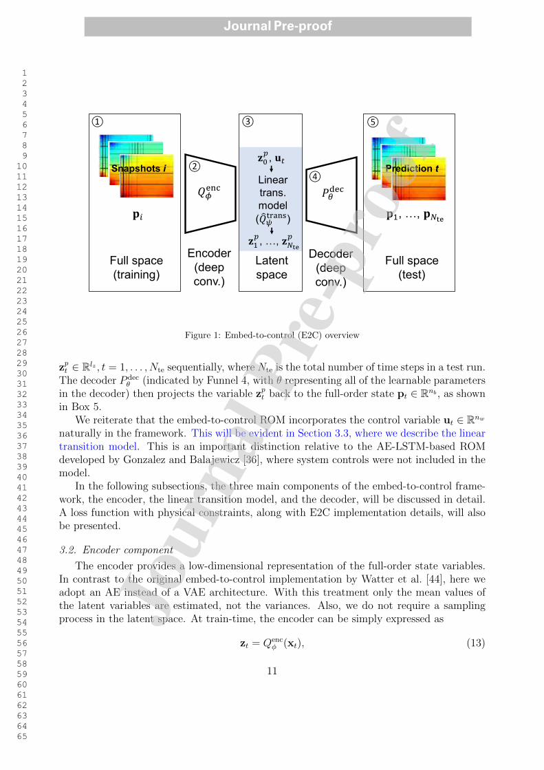
3.1. E2C overview

The embed-to-control framework entails three processing steps: an encoder or inferencemodel that projects the system variables from a high-dimensional space to a low-dimensionalsubspace (referred to here as the latent space), a linear transition model that approximatessystem dynamics in low-dimension, and a decoder or generative model that projects solu-tions back to high-dimensional (full-order) space. The E2C framework originally proposedby Watter et al. [44] used a VAE architecture for both the encoder and decoder procedures,which allowed them to account for uncertainty in predictions. In the formulation here, theVAE architecture is reduced to an auto-encoder (AE) architecture, since we are consideringdeterministic systems. We performed limited numerical experimentation (some of the resultsfrom these experiments are presented in Supplementary Material) and found that AE wasmore accurate than VAE for our application. This may be because the complexity of thenetwork has not reached the point where over-fitting is a significant issue. If we use deepernetworks, as might be required if we wish to use the E2C ROM for production optimiza-tion under uncertainty, another comparison between AE and VAE should be performed todetermine the preferable architecture.

We note that the AE architecture is commonly used for semantic segmentation [47],where each pixel of the image is associated with a class label, and for depth prediction [48],where the 3D geometry of a scene is inferred from a 2D image. In the context of subsurfaceflow simulation, AE architectures have been used to construct surrogate simulation modelsas an image-to-image regression. In this case the input images are reservoir properties (e.g.,permeability field) and the outputs are state variables [29, 30].

Figure 1 displays the overall workflow for our embed-to-control model. The pressure fieldpi ∈ Rnb is the only state variable shown in this illustration (the subscript i, distinct fromt, denotes the time steps in a training run), though our actual problem also includes thesaturation field Si ∈ Rnb . Additional state variables would appear in more general settings(e.g., displacements if a coupled flow-geomechanics model is considered).

Box 1 in Fig. 1 displays pressure snapshots pi ∈ Rnb , i = 1, . . . , Ns in the full-orderspace, where Ns is the total number of snapshots. The notation Qenc

φ in Funnel 2 denotesthe encoder, which projects the full space into a latent space, with φ representing all of the‘learnable’ parameters in the encoder. By learnable parameters we mean, in general, theset of parameters within the deep-learning-based ROM that are determined in the offlinetraining step. This training is accomplished by minimizing an appropriate loss function.As discussed later, there are learnable parameters associated with the encoder, decoder,and linear transition components of the ROM. The variable zpi ∈ Rlz in Box 3 is the latentvariable for pressure, with lz the dimension of the latent space.

In Box 3, the test simulation results are approximated in the latent space with a lineartransition model. The variable zp0 ∈ Rlz denotes the initial latent state for a test run,and ut ∈ Rnw , t = 1, . . . , Nctrl designates the control sequence for a test run, with nw thenumber of wells (as noted previously), the subscript t indicates time step in the test run,and Nctrl is the number of control steps in the test run. The linear transition model Qtrans

ψ

(ψ denotes the learnable parameters) takes zp0 ∈ Rlz and ut ∈ Rnw as input, and outputs

10

Jour

nal P

re-p

roof

Journal Pre-proof

1

2

3

4

5

6

7

8

9

10

11

12

13

14

15

16

17

18

19

20

21

22

23

24

25

26

27

28

29

30

31

32

33

34

35

36

37

38

39

40

41

42

43

44

45

46

47

48

49

50

51

52

53

54

55

56

57

58

59

60

61

62

63

64

65

Snapshots i𝐳0𝑝, 𝐮𝑡Linear

trans.

model

( 𝑄𝜓trans)𝐳1𝑝, …, 𝐳𝑁te𝑝Full space

(training)

Full space

(test)

𝐩𝑖 𝐩1, …, 𝐩𝑁tePrediction t

Encoder

(deep

conv.)

Decoder

(deep

conv.)

𝑄𝜙enc 𝑃𝜃decLatent

space

①

②

③

④

⑤

Figure 1: Embed-to-control (E2C) overview

zpt ∈ Rlz , t = 1, . . . , Nte sequentially, where Nte is the total number of time steps in a test run.The decoder P dec

θ (indicated by Funnel 4, with θ representing all of the learnable parametersin the decoder) then projects the variable zpt back to the full-order state pt ∈ Rnb , as shownin Box 5.

We reiterate that the embed-to-control ROM incorporates the control variable ut ∈ Rnw

naturally in the framework. This will be evident in Section 3.3, where we describe the lineartransition model. This is an important distinction relative to the AE-LSTM-based ROMdeveloped by Gonzalez and Balajewicz [36], where system controls were not included in themodel.

In the following subsections, the three main components of the embed-to-control frame-work, the encoder, the linear transition model, and the decoder, will be discussed in detail.A loss function with physical constraints, along with E2C implementation details, will alsobe presented.

3.2. Encoder component

The encoder provides a low-dimensional representation of the full-order state variables.In contrast to the original embed-to-control implementation by Watter et al. [44], here weadopt an AE instead of a VAE architecture. With this treatment only the mean values ofthe latent variables are estimated, not the variances. Also, we do not require a samplingprocess in the latent space. At train-time, the encoder can be simply expressed as

zt = Qencφ (xt), (13)

11

Jour

nal P

re-p

roof

Journal Pre-proof

1

2

3

4

5

6

7

8

9

10

11

12

13

14

15

16

17

18

19

20

21

22

23

24

25

26

27

28

29

30

31

32

33

34

35

36

37

38

39

40

41

42

43

44

45

46

47

48

49

50

51

52

53

54

55

56

57

58

59

60

61

62

63

64

65

where Qencφ represents the encoder (this notation appears in Fig. 1). The variable xt ∈ R2nb is

the full-order state variable at time step t, and zt ∈ Rlz is the corresponding latent variable,with lz the dimension of the latent space.

In the examples presented later, we consider a 2D 60× 60 oil-water model (which meansthe full-order system is of dimension 7200), and we set lz = 50. This value of lz wasdetermined based on numerical experiments, where the goal was to assure that the dimensionof the subspace was high enough to accurately represent the physics, while still low enoughfor efficient computation. More specifically, the initial value of lz was set consistent withvalues used in POD-TPWL [19, 20], where lz is typically on the order of 100. Then, lz wasreduced gradually, with the accuracy of the E2C ROM monitored. Non-negligible reductionin E2C accuracy was observed for lz < 50; thus we use lz = 50 in this work. Note that theappropriate value for lz is expected to be somewhat case-dependent. Cross-validation wasalso conducted to verify that the trained network did not lead to over-fitting.

Note that Eq. 13 is analogous to Eq. 3 in the POD-TPWL procedure, except the linearprojection in POD is replaced by a nonlinear projection Qenc

φ in the encoder. Followingthe convention described earlier, we use variables without a ‘hat’ to denote (projected) truesolutions of Eq. 2, which are available from training runs. Variables with a hat designateapproximate solutions provided by the test-time ROM.

The detailed layout of the encoder in the E2C model is presented in Fig. 2. During train-ing, sequences of pressure and saturation snapshots are fed through the encoder network,and sequences of latent state variables zt ∈ Rlz are generated. The encoder network usedhere is comprised of a stack of four encoding blocks, a stack of three residual convolutional(resConv) blocks, and a dense layer. The encoder in Fig. 2 is more complicated (i.e., itcontains resConv blocks and has more convolutional layers) compared to those used in [44].A more complicated structure may be needed here because, compared to the prototype plan-ning tasks addressed in [44] (e.g, cart-pole balancing, and three-link robotic arm planning),proper representation of PDE-based pressure and saturation fields requires feature mapsfrom a deeper network.

Similar to the CNN-PCA proposed by Liu et al. [26], which uses the filter operations inCNN to capture the spatial correlations that characterize geological features, the embed-to-control framework uses stacks of convolutional filters to represent the spatial distribution ofthe pressure and saturation fields determined by the underlying governing equations. Earlierimplementations with AE/VAE-based ROMs [31, 36] have demonstrated the potential ofconvolutional filters to capture such fields in fluid dynamics problems. Thus, our encodernetwork is mostly comprised of these convolutional filters (in the form of two-dimensionalconvolutional layers, i.e., conv2D layer [49]). More detail on the encoder network is providedin Table 1 in Supplementary Material.

The input to an encoding block is first fed through a convolution operation, which can alsobe viewed as a linear filter. Following the expression in [26], the mathematical formulationof linear filtering is

Fi,j(x) =n∑

p=−n

n∑

q=−nwp,qxi+p,j+q + b, (14)

12

Jour

nal P

re-p

roof

Journal Pre-proof

1

2

3

4

5

6

7

8

9

10

11

12

13

14

15

16

17

18

19

20

21

22

23

24

25

26

27

28

29

30

31

32

33

34

35

36

37

38

39

40

41

42

43

44

45

46

47

48

49

50

51

52

53

54

55

56

57

58

59

60

61

62

63

64

65

Encoder Network

S1

S2

p1

p2

z2

Calculate

reconstruction loss

together with Decoder

ResConv Block

Encoding Block

Dense Layer

Dim: nb = nx x ny

Dim: lz << nb

z1

Figure 2: Encoder layout

where x is the input state map, subscripts i and j denote x and y coordinate directionindices, w represents the weights of a linear filter (template) of size (2n+1)×(2n+1), Fi,j(x)designates the filter response map (i.e., feature map) for x at spatial location (i, j), and b isa scalar parameter referred to as bias. Note that there are typically many filters associatedwith a conv2D layer, and the filter response map, which collects all of these operations, isthus a third-order tensor. The output filter response maps are then passed through a batchnormalization (batchNorm) layer [50], which applies normalization operations (shifts themean to zero and rescales by the standard deviation) for each subset of training data. AbatchNorm operation is a crucial step in the efficient training of deep neural networks, sinceit renders the learning process less sensitive to parameter initialization, which means a largerinitial learning rate can be used. The nonlinear activation function ReLU (rectified linearunit, max(0,x)) [51] is applied on the normalized filter response maps to give a final response(output) of the encoder block. This nonlinear response is referred to as the ‘activation’ ofthe encoding block. The conv2D-batchNorm-ReLU architecture (with variation in ordering)is a standard processing step in CNNs.

The learnable parameters in an encoding block include the collection of weights w andbias terms b in Eq. 14 for all of the filters in conv2D layers, and the shifting and scalingparameters in batchNorm. These parameters are determined during training by minimizingthe loss function (defined later). The ReLU layer does not involve learnable parameters. Thecollection of learnable parameters in all the encoding blocks, resConv blocks, and dense layersin the encoder (which is about 2.42× 106 total parameters), is represented by φ in Eq. 13.An illustration of the encoding block structure is provided in Fig. 1(a) in Supplementary

13

Jour

nal P

re-p

roof

Journal Pre-proof

1

2

3

4

5

6

7

8

9

10

11

12

13

14

15

16

17

18

19

20

21

22

23

24

25

26

27

28

29

30

31

32

33

34

35

36

37

38

39

40

41

42

43

44

45

46

47

48

49

50

51

52

53

54

55

56

57

58

59

60

61

62

63

64

65

Material.To properly incorporate feature maps capable of representing the spatial pressure and

saturation distributions, as determined by the underlying governing equations, a deep neuralnetwork with many stacks of convolutional layers is required. Deep neural networks are,however, difficult to train, mostly due to the gradient vanishing issue [52]. By this wemean that gradients of the loss function with respect to the model parameters (weightsof the filters) become vanishingly small, which negatively impacts training. He et al. [53]addressed this issue by creating an additional identity mapping, referred to as resNet, thatbypasses the nonlinear layer. Following the idea of resNet, we add a stack of resConv blocksto the encoder network to deepen the network while mitigating the vanishing-gradient issue.The nonlinear layer in the resConv block still generally follows the conv2D-batchNorm-ReLUarchitecture. See Fig. 1(d) in Supplementary Material for a depiction of the resConv block.

Similar to that of the encoding block, the output of resConv blocks is a stack of low-dimension feature maps. This stack of feature maps is ‘flattened’ to a vector (which is still arelatively high-dimensional vector due to the large number of feature maps), and then inputto a dense layer. A dense (fully-connected) layer is simply a linear projection that maps ahigh-dimensional vector to a low-dimensional vector.

The overall architecture of the encoder network used here differs from that constructedby Zhu and Zabaras [29] in three key aspects. First, resNet is used in our encoder while theyused denseNet [54] to mitigate the vanishing-gradient issue. Another key distinction is thatthe encoder (and the decoder) in [29] do not include the dense layer at the end, which meansthe encoder outputs a stack of feature maps at the end. A large number of feature maps(i.e., a tall but relatively thin third-order tensor) would be too high-dimensional for thesequential linear operations subsequently performed by our linear transition model. Finally,Zhu and Zabaras [29] adopted a U-Net [47] architecture, while our E2C model uses a differentarchitecture.

The encoder (and decoder) in the embed-to-control ROM is analogous to the PODrepresentation used in POD-TPWL. As noted earlier, the basis matrix Φ constructed viaSVD of the snapshot matrices has the feature that it minimizes eproj in Eq. 9. In the contextof the encoder, a reconstruction loss LR, which is similar to eproj for POD, is computed.Conceptually, the ‘best’ Qenc

φ is found by minimizing LR. However, as mentioned earlier,the optimization applied for the embed-to-control model involves all three processing stepsconsidered together, so LR is not minimized separately.

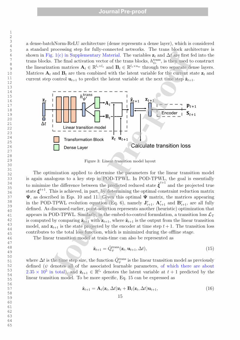
3.3. Linear transition model

The linear transition model evolves the latent variable from one time step to the next,given the controls. Fig. 3 shows how the linear transition model is constructed and evaluatedduring the offline stage (train-time). The inputs to the linear transition model include thelatent variable for the current state zt ∈ Rlz , the current step control ut+1 ∈ Rnw , andtime step size ∆t. The model outputs the predicted latent state for the next time stepzt+1 ∈ Rlz . We reiterate that zt+1 represents the output of the linear transition model. Thestructure of the linear transition model, which generally follows that in [44], is comprised ofa stack of three transformation (trans) blocks and two dense layers. The trans block follows

14

Jour

nal P

re-p

roof

Journal Pre-proof

1

2

3

4

5

6

7

8

9

10

11

12

13

14

15

16

17

18

19

20

21

22

23

24

25

26

27

28

29

30

31

32

33

34

35

36

37

38

39

40

41

42

43

44

45

46

47

48

49

50

51

52

53

54

55

56

57

58

59

60

61

62

63

64

65

a dense-batchNorm-ReLU architecture (dense represents a dense layer), which is considereda standard processing step for fully-connected networks. The trans block architecture isshown in Fig. 1(c) in Supplementary Material. The variables zt and ∆t are first fed into thetrans blocks. The final activation vector of the trans blocks, htransψ′ , is then used to construct

the linearization matrices At ∈ Rlz×lz and Bt ∈ Rlz×nw through two separate dense layers.Matrices At and Bt are then combined with the latent variable for the current state zt andcurrent step control ut+1 to predict the latent variable at the next time step zt+1.

Linear transition model

Calculate transition lossTransformation Block

Dense Layer

𝐳𝑡 ො𝐳𝑡+1

𝐮𝑡+1

𝐳𝑡+1Encoder

𝐩𝑡+1𝐒𝑡+1Δ𝑡ℎ𝜓′trans 𝐀𝑡

𝐳𝑡𝐁𝑡

Figure 3: Linear transition model layout

The optimization applied to determine the parameters for the linear transition modelis again analogous to a key step in POD-TPWL. In POD-TPWL, the goal is essentially

to minimize the difference between the predicted reduced state ξt+1

and the projected truestate ξt+1. This is achieved, in part, by determining the optimal constraint reduction matrixΨ, as described in Eqs. 10 and 11. Given this optimal Ψ matrix, the matrices appearingin the POD-TPWL evolution equation (Eq. 6), namely Jri+1, A

ri+1 and Br

i+1, are all fullydefined. As discussed earlier, point-selection represents another (heuristic) optimization thatappears in POD-TPWL. Similarly, in the embed-to-control formulation, a transition loss LT

is computed by comparing zt+1 with zt+1, where zt+1 is the output from the linear transitionmodel, and zt+1 is the state projected by the encoder at time step t+1. The transition losscontributes to the total loss function, which is minimized during the offline stage.

The linear transition model at train-time can also be represented as

zt+1 = Qtransψ (zt,ut+1,∆t), (15)

where ∆t is the time step size, the function Qtransψ is the linear transition model as previously

defined (ψ denotes all of the associated learnable parameters, of which there are about2.35 × 105 in total), and zt+1 ∈ Rlz denotes the latent variable at t + 1 predicted by thelinear transition model. To be more specific, Eq. 15 can be expressed as

zt+1 = At(zt,∆t)zt +Bt(zt,∆t)ut+1, (16)

15

Jour

nal P

re-p

roof

Journal Pre-proof

1

2

3

4

5

6

7

8

9

10

11

12

13

14

15

16

17

18

19

20

21

22

23

24

25

26

27

28

29

30

31

32

33

34

35

36

37

38

39

40

41

42

43

44

45

46

47

48

49

50

51

52

53

54

55

56

57

58

59

60

61

62

63

64

65

where At ∈ Rlz×lz and Bt ∈ Rlz×nw are matrices. Consistent with the expressions in [44],these matrices are given by

vec[At] = WAhtransψ′ (zt,∆t) + bA, (17)

vec[Bt] = WBhtransψ′ (zt,∆t) + bB, (18)

where vec denotes vectorization, so vec[At] ∈ R(l2z)×1 and vec[Bt] ∈ R(lznw)×1. The variablehtransψ′ ∈ Rntrans represents the final activation output after three transformation blocks (whichaltogether are referred to as the transformation network). The ψ′ in Eqs. 17 and 18 is asubset of ψ in Eq. 15, since the latter also includes parameters outside the transformationnetwork. Here WA ∈ Rl2z×ntrans , WB ∈ R(lznw)×ntrans , bA ∈ R(l2z)×1, and bB ∈ R(lznw)×1,where ntrans denotes the dimension of the transformation network. We set ntrans = 200 inthe model tested here.

During the online stage (test-time) the linear transition model is slightly different, sincethe latent variable fed into the model (zt ∈ Rlz) is predicted from the last time step.Therefore, at test-time, Eq. 16 becomes

zt+1 = At(zt,∆t)zt +Bt(zt,∆t)ut+1. (19)

Note the only difference is that zt on the right-hand side of Eq. 16 is replaced by zt in Eq. 19.The test-time formulation of the linear transition model is directly analogous to the

linear representation step in POD-TPWL. In POD-TPWL, since the training step i (andthus i+ 1) is determined based on the point-selection calculation involving ξt, the matricesappearing in the online expression (Eq. 8) can be considered to be functions of ξt. Aftersome reorganization, Eq. 8 can then be written as

ξt+1

= ATPWLt (ξt)ξt +BTPWL

t (ξt)ut+1 + cTPWLt , (20)

whereATPWLt = −(Ji+1

r )−1Ai+1r , BTPWL

t = −(Ji+1r )−1Ui+1

r ,

cTPWLt = −ATPWL

t ξi −BTPWLt ui+1 + ξi+1.

(21)

Thus we see that Eq. 19 for the online stage of the embed-to-control formulation is of thesame form as Eq. 20 for the online stage of POD-TPWL. The key difference is that matricesAt and Bt in E2C are determined by a deep-learning model instead of being constructedfrom derivative matrices from training runs. The vector ct does not appear in the E2Cformulation, since this representation does not entail expansion around nearby solutions.

Note that the transition loss used here involves pairs of time steps (t and t+1) rather thanthe full sequence. Approaches of this type can potentially lead to error accumulation over thefull simulation period. As will be demonstrated later (in the results), error accumulationis not significant for the cases considered here, though this is something that should bemonitored. Alternate treatments for the transition loss, in which the loss function is definedover the entire simulation period, are presented in [32]. Using approaches of this type, error

16

Jour

nal P

re-p

roof

Journal Pre-proof

1

2

3

4

5

6

7

8

9

10

11

12

13

14

15

16

17

18

19

20

21

22

23

24

25

26

27

28

29

30

31

32

33

34

35

36

37

38

39

40

41

42

43

44

45

46

47

48

49

50

51

52

53

54

55

56

57

58

59

60

61

62

63

64

65

propagation over time can be effectively controlled. The formulation in [32] is, however, forcases with fixed well settings. It is not clear if this approach can be applied directly for caseswith time-varying well controls, as are considered here.

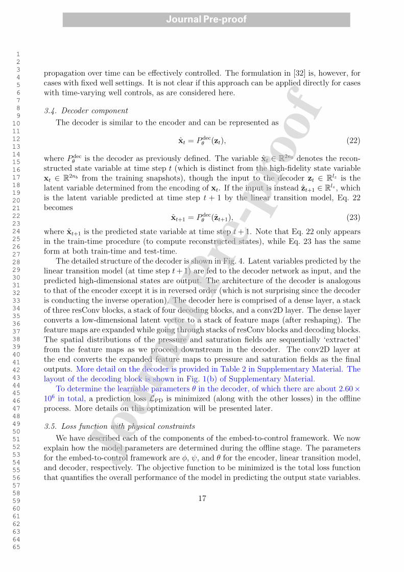
3.4. Decoder component

The decoder is similar to the encoder and can be represented as

xt = P decθ (zt), (22)

where P decθ is the decoder as previously defined. The variable xt ∈ R2nb denotes the recon-

structed state variable at time step t (which is distinct from the high-fidelity state variablext ∈ R2nb from the training snapshots), though the input to the decoder zt ∈ Rlz is thelatent variable determined from the encoding of xt. If the input is instead zt+1 ∈ Rlz , whichis the latent variable predicted at time step t + 1 by the linear transition model, Eq. 22becomes

xt+1 = P decθ (zt+1), (23)

where xt+1 is the predicted state variable at time step t+ 1. Note that Eq. 22 only appearsin the train-time procedure (to compute reconstructed states), while Eq. 23 has the sameform at both train-time and test-time.

The detailed structure of the decoder is shown in Fig. 4. Latent variables predicted by thelinear transition model (at time step t+1) are fed to the decoder network as input, and thepredicted high-dimensional states are output. The architecture of the decoder is analogousto that of the encoder except it is in reversed order (which is not surprising since the decoderis conducting the inverse operation). The decoder here is comprised of a dense layer, a stackof three resConv blocks, a stack of four decoding blocks, and a conv2D layer. The dense layerconverts a low-dimensional latent vector to a stack of feature maps (after reshaping). Thefeature maps are expanded while going through stacks of resConv blocks and decoding blocks.The spatial distributions of the pressure and saturation fields are sequentially ‘extracted’from the feature maps as we proceed downstream in the decoder. The conv2D layer atthe end converts the expanded feature maps to pressure and saturation fields as the finaloutputs. More detail on the decoder is provided in Table 2 in Supplementary Material. Thelayout of the decoding block is shown in Fig. 1(b) of Supplementary Material.

To determine the learnable parameters θ in the decoder, of which there are about 2.60×106 in total, a prediction loss LPD is minimized (along with the other losses) in the offlineprocess. More details on this optimization will be presented later.

3.5. Loss function with physical constraints

We have described each of the components of the embed-to-control framework. We nowexplain how the model parameters are determined during the offline stage. The parametersfor the embed-to-control framework are φ, ψ, and θ for the encoder, linear transition model,and decoder, respectively. The objective function to be minimized is the total loss functionthat quantifies the overall performance of the model in predicting the output state variables.

17

Jour

nal P

re-p

roof

Journal Pre-proof

1

2

3

4

5

6

7

8

9

10

11

12

13

14

15

16

17

18

19

20

21

22

23

24

25

26

27

28

29

30

31

32

33

34

35

36

37

38

39

40

41

42

43

44

45

46

47

48

49

50

51

52

53

54

55

56

57

58

59

60

61

62

63

64

65

Decoder Network

Calculate

prediction loss

ResConv Block

Decoding Block

Dense Layer

Dim: nb = nx x ny

Dim: lz << nbො𝐳2 ො𝐳3ෝ𝐩2ෝ𝐩3

𝐒2𝐒3

2D Conv. Layer

Figure 4: Decoder layout

We have briefly introduced the reconstruction loss (LR), the linear transition loss (LT),and the prediction loss (LPD), which comprise major components of the total loss function.To be more specific, the reconstruction loss for a training data point i can be expressed as

(LR)i = {‖xt − xt‖22}i, (24)

where i = 1, . . . , Nt, with Nt denoting the total number of data points generated in thetraining runs. Note that Nt = Ns − ntrain, where Ns is the total number of snapshots in thetraining runs and ntrain is the number of training simulations performed. Here Nt and Ns

differ because, for a training simulation containing Ntr snapshots, only Ntr − 1 data pointscan be collected (since pairs of states, at sequential time steps, are required). The variablext is the state variable at time step t from a training simulation, and xt = P dec

θ (zt) =P decθ (Qenc

φ (xt)) denotes the states reconstructed by the encoder and decoder.The linear transition loss for training point i is similarly defined as

(LT)i = {‖zt+1 − zt+1‖22}i, (25)

where zt+1 = Qencφ (xt+1) is the latent variable encoded from the full-order state variable at

t + 1, and the variable zt+1 = Qtransψ (zt,ut+1,∆t) denotes the latent variable predicted by

the linear transition model. Finally, the prediction loss for training point i is defined as

(LPD)i = {‖xt+1 − xt+1‖22}i, (26)

18

Jour

nal P

re-p

roof

Journal Pre-proof

1

2

3

4

5

6

7

8

9

10

11

12

13

14

15

16

17

18

19

20

21

22

23

24

25

26

27

28

29

30

31

32

33

34

35

36

37

38

39

40

41

42

43

44

45

46

47

48

49

50

51

52

53

54

55

56

57

58

59

60

61

62

63

64

65

where xt+1 designates the state variable at time step t + 1 from the training simulations,and xt+1 = P dec

θ (zt+1) represents the full-order state variable predicted by the ROM. Thedata mismatch loss is the sum of these losses averaged over all training data points,

Ld =1

Nt

Nt∑

i=1

(LR)i + (LPD)i + λ(LT)i, (27)

where λ is a weight term.

4600

4800

5000

5200

5400

5600

5800

6000

(a) High-fidelity solution(HFStest)

4800

5000

5200

5400

5600

5800

6000

(b) ROM solutionwithout Lp

0

5

10

15

20

25

30

35

40

(c) |HFStest − ROMtest|without Lp (max error 97 psi)

4600

4800

5000

5200

5400

5600

5800

6000

(d) ROM solutionwith Lp

2

4

6

8

10

12

14

16

(e) |HFStest − ROMtest|with Lp (max error 16 psi)

Figure 5: Pressure field predictions with and without Lp (all colorbars in units of psi)

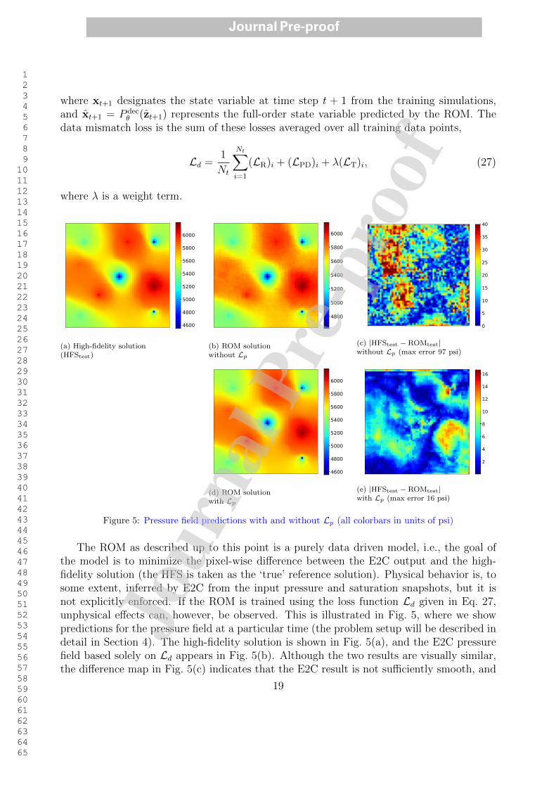
The ROM as described up to this point is a purely data driven model, i.e., the goal ofthe model is to minimize the pixel-wise difference between the E2C output and the high-fidelity solution (the HFS is taken as the ‘true’ reference solution). Physical behavior is, tosome extent, inferred by E2C from the input pressure and saturation snapshots, but it isnot explicitly enforced. If the ROM is trained using the loss function Ld given in Eq. 27,unphysical effects can, however, be observed. This is illustrated in Fig. 5, where we showpredictions for the pressure field at a particular time (the problem setup will be described indetail in Section 4). The high-fidelity solution is shown in Fig. 5(a), and the E2C pressurefield based solely on Ld appears in Fig. 5(b). Although the two results are visually similar,the difference map in Fig. 5(c) indicates that the E2C result is not sufficiently smooth, and

19

Jour

nal P

re-p

roof

Journal Pre-proof

1

2

3

4

5

6

7

8

9

10

11

12

13

14

15

16

17

18

19

20

21

22

23

24

25

26

27

28

29

30

31

32

33

34

35

36

37

38

39

40

41

42

43

44

45

46

47

48

49

50

51

52

53

54

55

56

57

58

59

60

61

62

63

64

65

relatively large errors appear at some spatial locations. This could have a significant impacton well rate predictions, which are an essential ROM output.

To address this issue, we combine the loss for data mismatch with a loss function basedon flow physics. Specifically, we seek to minimize the inconsistency in flux between eachpair of adjacent grid blocks. Extra weight is also placed on key well quantities. We considerboth reconstruction (at time step t) and prediction (at time step t+1). Thus we define thephysics-based loss for each data point, (Lp)i, as

(Lp)i ={‖k · [(∇pt −∇pt)recon + (∇pt+1 −∇pt+1)pred]‖22}i+ γ{‖(qwt − qwt )recon + (qwt+1 − qwt+1)pred‖22}i.

(28)

Here pt,pt+1 ∈ Rnb are the pressure fields at time steps t and t+ 1 from the training data,which are components of the state variables xt and xt+1, and pt, pt+1 ∈ Rnb represent theROM pressure reconstruction (at time step t, defined after Eq. 24) and prediction (at timestep t + 1, defined after Eq. 26). The variables qwt ,q

wt+1 ∈ Rnw are well quantities from the

training data, and qwt , qwt+1 ∈ Rnw are well quantities reconstructed (at time step t) and

predicted (at time step t+1) by the ROM. Recall that nw is the total number of wells. Thevariable γ is a parameter that defines the weights for well-data loss in loss function Lp. Thepressure gradients in Eq. 28 are computed via numerical finite difference. The additionalcomputation associated with these terms is negligible.

The terms on the right hand side of Eq. 28 correspond to the flux and source termsin Eq. 1. In the examples in this paper, we specify rates for injection wells and BHPsfor production wells. With this specification, the loss on injection rates is zero. The keyquantity to track for production wells is the well-block pressure for each well. This is becauseproduction rate is proportional to the difference between wellbore pressure (BHP in this case,which is specified) and well-block pressure. The proportionality coefficient is the product ofphase mobility λj and the Peaceman well index [55], which depends on permeability, blockdimensions and wellbore radius. Because overall well rate in this case is largely impacted bywell-block pressure, we set the second term on the right-hand side of Eq. 28 to γ′‖pwj − pwj ‖22,where pwj ∈ Rnp and pwj ∈ Rnp (j = t, t+ 1) denote the true and ROM well-block pressures,and np is the number of production wells. Here γ′ is a modified weight that accounts for thewell index.

The physics-based loss function is computed by averaging (Lp)i over all data points, i.e.,

Lp =1

Nt

Nt∑

i=1

(Lp)i. (29)

Combining the loss for data mismatch with this physics-based loss, the total loss functionbecomes

L = Ld + αLp, (30)

where α is a weight term. Through limited numerical experimentation, we found α = 0.033and γ′ = 20 to be appropriate values for these parameters. The E2C ROM prediction for

20

Jour

nal P

re-p

roof

Journal Pre-proof

1

2

3

4

5

6

7

8

9

10

11

12

13

14

15

16

17

18

19

20

21

22

23

24

25

26

27

28

29

30

31

32

33

34

35

36

37

38

39

40

41

42

43

44

45

46

47

48

49

50

51

52

53

54

55

56

57

58

59

60

61

62

63

64

65

the pressure field at a particular time, using the total loss function L, is shown in Fig. 5(d),and the difference map appears in Fig. 5(e). We see that the ROM prediction is noticeablyimproved when Lp is included in the loss function. Specifically, the maximum pressure erroris reduced from 97 psi to 16 psi, and the resulting field is smoother (and thus more physical).This demonstrates the benefit of incorporating physics-based losses into the E2C ROM. Wenote that the (global) flux-loss terms in Eq. 28 contribute more to this error reduction thanthe well-block-loss terms.

3.6. E2C implementation and training details

To train the E2C model, we use a data set D = {(xt,xt+1,ut+1)i}, i = 1, . . . , Nt, contain-ing full-order states and corresponding well controls, where Nt is the total number of trainingrun data points. In the examples in this paper, we simulate a total of 300 training runs. Asdiscussed earlier, this is many more than are used with POD-TPWL (where we typicallysimulate three or five training runs), but we expect a much higher degree of robustness withE2C. By this we mean that E2C can provide accurate results over a large range of controlspecifications, rather than over a limited range as in POD-TPWL.

Part of the reason we use a large number of full-order training simulations with the E2CROM is that the pressure and saturation solutions (snapshots) are extracted at only 20time steps in each simulation run. These time steps correspond to control steps (changesin well controls). Thus we set Nctrl = Ntr = Nte = 20. This treatment accelerates trainingand focuses ROM predictions on quantities of interest at time steps when the controls arechanging. With 300 training runs, this provides a total number of data points of Nt = 5700.It is possible, however, that fewer total training runs could be used if we extracted solutionsat more time steps. This might have the downside of limiting the variability in the trainingdata, so a balance between the number of runs and the number of solutions extracted fromeach run must be established. This issue should be considered in future work. We notefinally that the training runs are completely independent of one another, so they can beperformed in parallel if a large cluster or cloud computing is available.

The gradient of the total loss function with respect to the model parameters (φ, ψ, θ)is calculated via back-propagation through the embed-to-control framework. The adaptivemoment estimation (ADAM) algorithm is used for this optimization, as it has been provento be effective for optimizing deep neural networks [56]. The rate at which the modelparameters are updated at each iteration is controlled by the learning rate lr. Here we setlr = 10−4.

Normalization is an important data preprocessing step, and its appropriate applicationcan improve both the learning process and output quality. For saturation we have S ∈ [0, 1],so normalization is not required. Pressure and well data, including control variables, arenormalized. Normalized rate q0, and pressure (both grid-block pressure and BHP) p0, aregiven by

q0 =q − qmin

qmax − qmin

, p0 =p− pmin

pmax − pmin

. (31)

Here q denotes simulator rate output in units of m3/day, qmax and qmin are the upper andlower injection-rate bounds, p is either grid-block pressure or production-well BHP (units of

21

Jour

nal P

re-p

roof

Journal Pre-proof

1

2

3

4

5

6

7

8

9

10

11

12

13

14

15

16

17

18

19

20

21

22

23

24

25

26

27

28

29

30

31

32

33

34

35

36

37

38

39

40

41

42

43

44

45

46

47

48

49

50

51

52

53

54

55

56

57

58

59

60

61

62

63

64

65

psi or bar), pmin is the lower bound on BHP, and pmax is 1.1 times the highest field pressureobserved (the factor of 1.1 ensures essentially all data fall within the range).

Algorithm 1: E2C ROM procedures

Procedure: Offline procedure1 Perform training simulations with given control settings;2 Collect snapshots xt and controls ut and normalize with Eq. 31;3 Construct training dataset D;4 for each training epoch do

5 Feed the training dataset through E2C model (i.e., Qφ, Qψ, and Pθ defined inEqs. 13, 16 and 22);

6 Compute loss function L defined in Eq. 30;7 Get derivatives of L with respect to (φ, ψ, θ);8 Update (φ, ψ, θ);

9 endProcedure: Online procedure

10 Construct E2C model with parameters (φ, ψ, θ) determined in the offline procedure;11 Initialize predicted value x0 = x0;12 for t = 1, . . . , T (final simulation time) do13 Predict xt+1 from xt with E2C model defined in Eqs. 13, 19 and 23;14 end15 Compute well quantities and perform any subsequent analysis;

The workflows for the offline and online components of the E2C ROM are summarized inAlgorithm 1. In terms of timing, each full-order training simulation requires about 60 secondsto run on dual Intel Xeon ES-2670 CPUs (24 cores). Our E2C ROM is implemented usingKeras [57] with TensorFlow [58] backend. The offline training process (excluding trainingsimulation runtime) takes around 10-12 minutes on a Tesla V100 GPU node (exact timingsdepend on the memory allocated, which can vary from 8-12 GB). The model is applied on100 test runs, which will be discussed in detail in the following section. Nearly all of the testresults presented are based on the use of 300 training runs, though we also present summaryerror statistics using 100 and 200 training runs. Offline training for these cases requiresabout the same amount of time as for 300 training runs, except for the direct savings in thefull-order training simulations.

4. Results using embed-to-control ROM

In this section, we describe the model setup for the oil-water simulations and we presentsimulation results for the deep-learning-based ROM. One of the test cases is considered indetail in this section; results for two additional test cases are provided in SupplementaryMaterial. In this section we also present summary error results for all 100 test cases.

22

Jour

nal P

re-p

roof

Journal Pre-proof

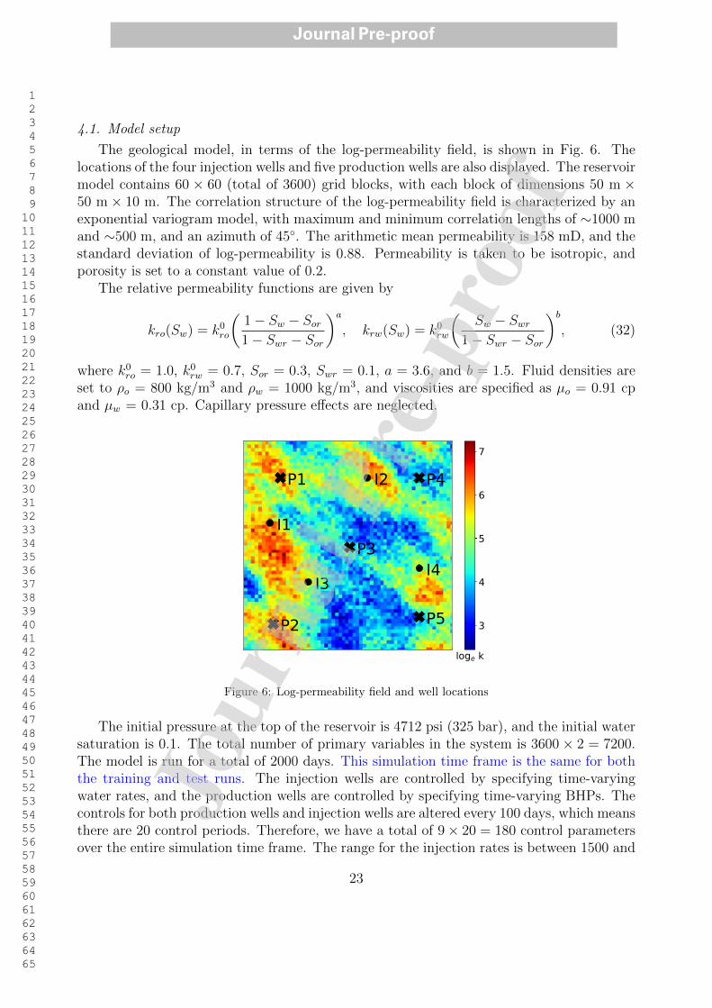
1

2

3

4

5

6

7

8

9

10

11

12

13

14

15

16

17

18

19

20

21

22

23

24

25

26

27

28

29

30

31

32

33

34

35

36

37

38

39

40

41

42

43

44

45

46

47

48

49

50

51

52

53

54

55

56

57

58

59

60

61

62

63

64

65

4.1. Model setup

The geological model, in terms of the log-permeability field, is shown in Fig. 6. Thelocations of the four injection wells and five production wells are also displayed. The reservoirmodel contains 60 × 60 (total of 3600) grid blocks, with each block of dimensions 50 m ×50 m× 10 m. The correlation structure of the log-permeability field is characterized by anexponential variogram model, with maximum and minimum correlation lengths of ∼1000 mand ∼500 m, and an azimuth of 45◦. The arithmetic mean permeability is 158 mD, and thestandard deviation of log-permeability is 0.88. Permeability is taken to be isotropic, andporosity is set to a constant value of 0.2.

The relative permeability functions are given by

kro(Sw) = k0ro

(1− Sw − Sor1− Swr − Sor

)a

, krw(Sw) = k0rw

(Sw − Swr

1− Swr − Sor

)b

, (32)

where k0ro = 1.0, k0rw = 0.7, Sor = 0.3, Swr = 0.1, a = 3.6, and b = 1.5. Fluid densities areset to ρo = 800 kg/m3 and ρw = 1000 kg/m3, and viscosities are specified as µo = 0.91 cpand µw = 0.31 cp. Capillary pressure effects are neglected.

P1

P2

P3

P4

P5

I1

I2

I3I4

loge k

3

4

5

6

7

Figure 6: Log-permeability field and well locations

The initial pressure at the top of the reservoir is 4712 psi (325 bar), and the initial watersaturation is 0.1. The total number of primary variables in the system is 3600× 2 = 7200.The model is run for a total of 2000 days. This simulation time frame is the same for boththe training and test runs. The injection wells are controlled by specifying time-varyingwater rates, and the production wells are controlled by specifying time-varying BHPs. Thecontrols for both production wells and injection wells are altered every 100 days, which meansthere are 20 control periods. Therefore, we have a total of 9× 20 = 180 control parametersover the entire simulation time frame. The range for the injection rates is between 1500 and

23

Jour

nal P

re-p

roof

Journal Pre-proof

1

2

3

4

5

6

7

8

9

10

11

12

13

14

15

16

17

18

19

20

21

22

23

24

25

26

27

28

29

30

31

32

33

34

35

36

37

38

39

40

41

42

43

44

45

46

47

48

49

50

51

52

53

54

55

56

57

58

59

60

61

62

63

64

65

6500 bbl/day (between 238 and 1033 m3/day). This is a very large range for well operationcompared with what is often considered with ROMs [19, 20]. The range for productionBHPs is 3770 to 3988 psi (between 260 and 275 bar).

The controls for the training and test runs are specified as follows. For each injection well,we randomly sample, from a uniform distribution between 2000 and 6000 bbl/day, a baselineinjection rate qbasew . Then, at each control period, we sample uniformly a perturbation q′wover the range [−500, 500] bbl/day. The rate for the control period is then prescribed tobe qbasew + q′w. Producer BHPs at each control step are sampled uniformly over the range[3770, 3988] psi. For production wells there is not a baseline BHP, and the settings fromcontrol step to control step are uncorrelated. This approach for specifying injection ratesresults in a wide range of solution behaviors (e.g., saturation distributions), since well-by-well injection varies considerably from run to run. This treatment also avoids the averagingeffect that can occur if injection rates are not referenced to a baseline value qbasew . Wellspecifications for a test case, generated using this procedure, are shown in Fig. 7.

We perform 300 training simulations to construct the E2C ROM, except where otherwiseindicated. As discussed in previous papers (e.g., [19]), the types of well schedules shownin Fig. 7 are intended to represent the well control profiles evaluated during optimizationprocedures, where the goal is to maximize oil production or profitability, or to minimizeenvironmental impact or some measure of risk. We note finally that the dimension of theE2C latent space, lz, is set to 50.

As discussed earlier, comparisons of E2C results with those from POD-TPWL are notperformed in this work. This is because the range over which the well settings are varied,and the number of training runs performed, are very different between the two procedures,so direct comparisons are not feasible. In particular, existing POD-TPWL implementationstypically involve 3–5 training runs, and relatively small perturbations in the test-run con-trols relative to those used in training runs (during optimization, retraining can be used withPOD-TPWL if necessary). Algorithmic treatments, specifically the point-selection strategyused to determine the solution around which linearization is performed, would require de-tailed reformulation if large numbers of training runs were used with POD-TPWL. With theE2C ROM, by contrast, the controls span a much broader range, but 100–300 training runsare required. In fact, as a deep-learning-based ROM, E2C requires, and is fully compatiblewith, large numbers of training runs. Thus, although there are conceptual similarities, thetwo approaches are distinct in terms of their pre-processing demands and applicability range,which greatly limits our ability to perform direct comparisons with current implementations.

4.2. Results for Test Case 1

In this section we present detailed results for a particular test case. These includewell quantities (injection BHPs and production rates) and global quantities (pressure andsaturation fields). The injection rate and BHP profiles for Test Case 1 are displayed inFig. 7. Here we show the water rates for the four injection wells (Fig. 7(a)-(d)), and theBHPs for the five production wells (Fig. 7(e)-(i)).

We now assess the performance of the deep-learning-based ROM for this test case. Thetime-evolution of the global saturation field is first considered. The first column in Fig. 8

24

Jour

nal P

re-p

roof

Journal Pre-proof

1

2

3

4

5

6

7

8

9

10

11

12

13

14

15

16

17

18

19

20

21

22

23

24

25

26

27

28

29

30

31

32

33

34

35

36

37

38

39

40

41

42

43

44

45

46

47

48

49

50

51

52

53

54

55

56

57

58

59

60

61

62

63

64

65

0 500 1000 1500 2000Time [day]

0.56

0.58

0.60

0.62

0.64

0.66

0.68

0.70

Inj r

ate

[100

0 m

3 /day

]

(a) Well I1

0 500 1000 1500 2000Time [day]

0.34

0.36

0.38

0.40

0.42

0.44

0.46

0.48

0.50

Inj r

ate

[100

0 m

3 /day

]

(b) Well I2

0 500 1000 1500 2000Time [day]

0.26

0.28

0.30

0.32

0.34

0.36

0.38

0.40

Inj r

ate

[100

0 m

3 /day

]

(c) Well I3

0 500 1000 1500 2000Time [day]

0.60

0.62

0.64

0.66

0.68

0.70

0.72

0.74

Inj r

ate

[100

0 m

3 /day

]

(d) Well I4

0 500 1000 1500 2000Time [day]

3775

3800

3825

3850

3875

3900

3925

3950

Prod

BHP

[psi]

(e) Well P1

0 500 1000 1500 2000Time [day]

3775

3800

3825

3850

3875

3900

3925

3950

3975

Prod

BHP

[psi]

(f) Well P2

0 500 1000 1500 2000Time [day]

3800

3825

3850

3875

3900

3925

3950

3975

Prod

BHP

[psi]

(g) Well P3

0 500 1000 1500 2000Time [day]

3800

3850

3900

3950

Prod

BHP

[psi]

(h) Well P4

0 500 1000 1500 2000Time [day]

3800

3850

3900

3950

Prod

BHP

[psi]

(i) Well P5

Figure 7: Test Case 1: well controls

25

Jour

nal P

re-p

roof

Journal Pre-proof

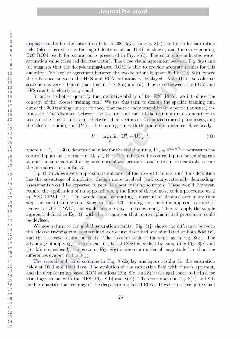
1

2

3

4

5

6

7

8

9

10

11

12

13

14

15

16

17

18

19

20

21

22

23

24

25

26

27

28

29

30

31

32

33

34

35

36

37

38

39

40

41

42

43

44

45

46

47

48

49

50

51

52

53

54

55

56

57

58

59

60

61

62

63

64

65

displays results for the saturation field at 200 days. In Fig. 8(a) the full-order saturationfield (also referred to as the high-fidelity solution, HFS) is shown, and the correspondingE2C ROM result for saturation is presented in Fig. 8(d). The color scale indicates watersaturation value (thus red denotes water). The close visual agreement between Fig. 8(a) and(d) suggests that the deep-learning-based ROM is able to provide accurate results for thisquantity. The level of agreement between the two solutions is quantified in Fig. 8(g), wherethe difference between the HFS and ROM solutions is displayed. Note that the colorbarscale here is very different than that in Fig. 8(a) and (d). The error between the ROM andHFS results is clearly very small.

In order to better quantify the predictive ability of the E2C ROM, we introduce theconcept of the ‘closest training run.’ We use this term to denote the specific training run,out of the 300 training runs performed, that most closely resembles (in a particular sense) thetest case. The ‘distance’ between the test run and each of the training runs is quantified interms of the Euclidean distance between their vectors of normalized control parameters, andthe ‘closest training run’ (k∗) is the training run with the minimum distance. Specifically,

k∗ = argmink

‖U0te −U0

tr,k‖22, (33)

where k = 1, . . . , 300, denotes the index for the training runs, Ute ∈ Rnw×Nctrl represents thecontrol inputs for the test run, Utr,k ∈ Rnw×Nctrl indicates the control inputs for training runk, and the superscript 0 designates normalized pressures and rates in the controls, as perthe normalizations in Eq. 31.

Eq. 33 provides a very approximate indicator of the ‘closest training run.’ This definitionhas the advantage of simplicity, though more involved (and computationally demanding)assessments would be expected to provide closer training solutions. These would, however,require the application of an approach along the lines of the point-selection procedure usedin POD-TPWL [19]. This would entail computing a measure of distance over many timesteps for each training run. Since we have 300 training runs here (as opposed to three orfive with POD-TPWL), this would become very time consuming. Thus we apply the simpleapproach defined in Eq. 33, with the recognition that more sophisticated procedures couldbe devised.

We now return to the global saturation results. Fig. 8(j) shows the difference betweenthe ‘closest training run’ (determined as we just described and simulated at high fidelity),and the test-case saturation fields. The colorbar scale is the same as in Fig. 8(g). Theadvantage of applying the deep-learning-based ROM is evident by comparing Fig. 8(g) and(j). More specifically, the error in Fig. 8(g) is about an order of magnitude less than thedifferences evident in Fig. 8(j).

The second and third columns in Fig. 8 display analogous results for the saturationfields at 1000 and 1800 days. The evolution of the saturation field with time is apparent,and the deep-learning-based ROM solutions (Fig. 8(e) and 8(f)) are again seen to be in closevisual agreement with the HFS (Fig. 8(b) and 8(c)). The error maps in Fig. 8(h) and 8(i)further quantify the accuracy of the deep-learning-based ROM. These errors are quite small

26

Jour

nal P

re-p

roof

Journal Pre-proof

1

2

3

4

5

6

7

8

9

10

11

12

13

14

15

16

17

18

19

20

21

22

23

24

25

26

27

28

29

30

31

32

33

34

35

36

37

38

39

40

41

42

43

44

45

46

47

48

49

50

51

52

53

54

55

56

57

58

59

60

61

62

63

64

65

0.2

0.3

0.4

0.5

0.6

(a) High-fidelity solution (HFStest) at200 days

0.2

0.3

0.4

0.5

0.6

(b) High-fidelity solution (HFStest) at1000 days

0.2

0.3

0.4

0.5

0.6

(c) High-fidelity solution (HFStest) at1800 days

0.2

0.3

0.4

0.5

0.6

(d) ROM solution (ROMtest) at 200days

0.2

0.3

0.4

0.5

0.6

(e) ROM solution (ROMtest) at 1000days

0.2

0.3

0.4

0.5

0.6

(f) ROM solution (ROMtest) at 1800days

0.00

0.02

0.04

0.06

0.08

0.10

0.12

0.14

(g) |HFStest − ROMtest| at 200 days

0.00

0.02

0.04

0.06

0.08

0.10

0.12

0.14

(h) |HFStest −ROMtest| at 1000 days

0.00

0.02

0.04

0.06

0.08

0.10

0.12

0.14

(i) |HFStest − ROMtest| at 1800 days

0.00

0.02

0.04

0.06

0.08

0.10

0.12

0.14

(j) |HFStest −HFStrain| at 200 days

0.00

0.02

0.04

0.06

0.08

0.10

0.12

0.14

(k) |HFStest −HFStrain| at 1000 days

0.00

0.02

0.04

0.06

0.08

0.10

0.12

0.14

(l) |HFStest −HFStrain| at 1800 days

Figure 8: Test Case 1: saturation field at 200, 1000 and 1800 days

27

Jour

nal P

re-p

roof

Journal Pre-proof

1

2

3

4

5

6

7

8

9

10

11

12

13

14

15

16

17

18

19

20

21

22

23

24

25

26

27

28

29

30

31

32

33

34

35

36

37

38

39

40

41

42

43

44

45

46

47

48

49

50

51

52

53

54

55

56

57

58

59

60

61

62

63

64

65

compared with the difference maps between the ‘closest training run’ and the HFS, shownin Fig. 8(k) and 8(l), which further illustrates the effectiveness of the ROM.

Note that in the ROM solutions, we do observe some local (unphysical) extrema withinthe saturation plumes. These are perhaps most apparent in Fig. 8(f), in the two lowerplumes. At the outer (bottom) edges of both plumes, we see small ‘islands’ of yellow pixelswithin a light green background. These local fluctuations correspond to nonmonotonicsaturation profiles, which are not observed in the HFS (see Fig. 8(c)). Smaller fluctuationsin similar regions can also be seen in Fig. 8(e). These unphysical extrema are a minor issuehere since the difference maps show small overall discrepancies between the ROM and high-fidelity solutions. In some cases, however, such fluctuations could be a cause for concern.A potential remedy for this would be to add a term to the physics-based loss function suchthat local extrema in saturation that are inconsistent with the governing flow equations arepenalized.

The global pressure field at particular times is also of interest. In Fig. 9(a) and (b) wedisplay the HFS and ROM pressure solutions at 1000 days. The close visual agreement sug-gests that the deep-learning-based ROM is able to provide accurate (and smooth) pressurepredictions. Fig. 9(c) shows the error map for the ROM solution, where we see that errorsare indeed very small. These errors are much less than those for the ‘closest training run,’which are shown in Fig. 9(d).

In many subsurface flow applications the well responses are of primary interest. E2CROM predictions for these quantities will now be assessed. Since in this problem we specifyinjection rates and production well BHPs, the quantities of interest are injection well BHPsand oil and water production rates. Figs. 10 and 11 display the phase flow rates for Wells P1and P2, which are the wells contributing most to total field production. Fig. 12 shows theBHP responses for all four injection wells. In all figures the black curves represent the full-order (reference) HFS, the red curves are the deep-learning-based ROM results, and the bluecurves are the results for the ‘closest training run.’ A high degree of accuracy between theROM and HFS results is consistently observed. The level of agreement in these essentialquantities is enhanced through the additional weighting placed on well-block quantities inloss function Lp (see Eq. 28).

We provide results for two more examples (Test Cases 2 and 3) in Supplementary Mate-rial. These results corroborate our observations here; namely, that the deep-learning-basedROM is able to accurately predict both global saturation and pressure distributions and wellquantities of interest.

Finally, we discuss the timings for the high-fidelity and ROM runs. The high-fidelitytest cases take 60 seconds each to simulate using AD-GPRS on a node with dual Intel XeonES-2670 CPUs (24 cores). The full batch of 100 test cases can be evaluated using the E2CROM in about 1.25 seconds on a Tesla V100 GPU node with 8 GB of memory allocated.A direct comparison thus indicates a speedup factor of 4800, though this value involvescomparing a GPU to a CPU. If we instead use the same CPU for the online E2C ROM runsas was used for the full-order simulations (Intel Xeon ES-2670), it takes around 16 secondsfor the 100 test runs. This corresponds to a speedup factor of 375, which is less than thatachieved with the GPU, but still very substantial.

28

Jour

nal P

re-p

roof

Journal Pre-proof

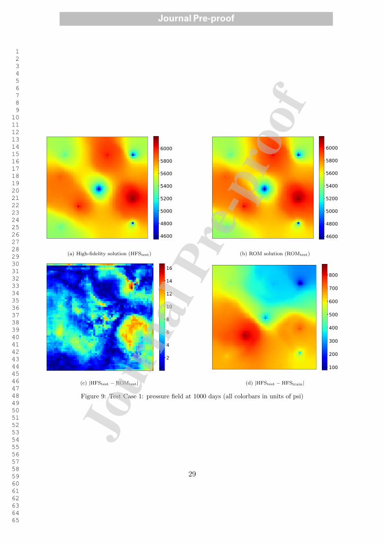
1

2

3

4

5

6

7

8

9

10

11

12

13

14

15

16

17

18

19

20

21

22

23

24

25

26

27

28

29

30

31

32

33

34

35

36

37

38

39

40

41

42

43

44

45

46

47

48

49

50

51

52

53

54

55

56

57

58

59

60

61

62

63

64

65

4600

4800

5000

5200

5400

5600

5800

6000

(a) High-fidelity solution (HFStest)

4600

4800

5000

5200

5400

5600

5800

6000

(b) ROM solution (ROMtest)

2

4

6

8

10

12

14

16

(c) |HFStest − ROMtest|

100

200

300

400

500

600

700

800

(d) |HFStest −HFStrain|

Figure 9: Test Case 1: pressure field at 1000 days (all colorbars in units of psi)

29

Jour

nal P

re-p

roof

Journal Pre-proof

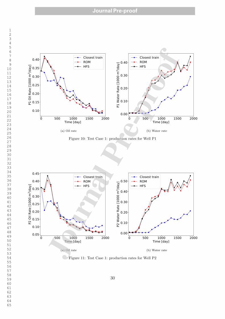
1

2

3

4

5

6

7

8

9

10

11

12

13

14

15

16

17

18

19

20

21

22

23

24

25

26

27

28

29

30

31

32

33

34

35

36

37

38

39

40

41

42

43

44

45

46

47

48

49

50

51

52

53

54

55

56

57

58

59

60

61

62

63

64

65

0 500 1000 1500 2000Time [day]

0.10

0.15

0.20

0.25

0.30

0.35

0.40

P1 O

il Ra

te [1

000

m3 /d

ay]

Closest trainROMHFS

(a) Oil rate

0 500 1000 1500 2000Time [day]

0.00

0.10

0.20

0.30

0.40

P1 W

ater

Rat

e [1

000

m3 /d

ay]

Closest trainROMHFS

(b) Water rate

Figure 10: Test Case 1: production rates for Well P1

0 500 1000 1500 2000Time [day]

0.05

0.10

0.15

0.20

0.25

0.30

0.35

0.40

0.45

P2 O

il Ra

te [1

000

m3 /d

ay]

Closest trainROMHFS

(a) Oil rate

0 500 1000 1500 2000Time [day]

0.00

0.10

0.20

0.30

0.40

0.50

P2 W

ater

Rat

e [1

000

m3 /d

ay]

Closest trainROMHFS

(b) Water rate

Figure 11: Test Case 1: production rates for Well P2

30

Jour

nal P

re-p

roof

Journal Pre-proof

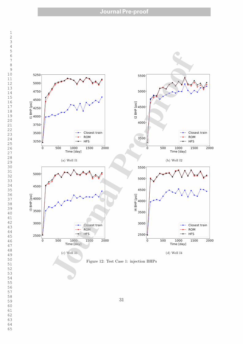
1

2

3

4

5

6

7

8

9

10

11

12

13

14

15

16

17

18

19

20

21

22

23

24

25

26

27

28

29

30

31

32

33

34

35

36

37

38

39

40

41

42

43

44

45

46

47

48

49

50

51

52

53

54

55

56

57

58

59

60

61

62

63

64

65

0 500 1000 1500 2000Time [day]

3250

3500

3750

4000

4250

4500

4750

5000

5250

I1 B

HP [p

si]

Closest trainROMHFS

(a) Well I1

0 500 1000 1500 2000Time [day]

3500

4000

4500

5000

5500

I2 B

HP [p

si]Closest trainROMHFS

(b) Well I2

0 500 1000 1500 2000Time [day]

2500

3000

3500

4000

4500

5000

I3 B

HP [p

si]

Closest trainROMHFS

(c) Well I3

0 500 1000 1500 2000Time [day]

2500

3000

3500

4000

4500

5000

5500

I4 B

HP [p

si]

Closest trainROMHFS

(d) Well I4

Figure 12: Test Case 1: injection BHPs

31

Jour

nal P

re-p

roof

Journal Pre-proof

1

2

3

4

5

6

7

8

9

10

11

12

13

14

15

16

17

18

19

20

21

22

23

24

25

26

27

28

29

30

31

32

33

34

35

36

37

38

39

40

41

42

43

44

45

46

47

48

49

50

51

52

53

54

55

56

57

58

59

60

61

62

63

64

65

4.3. Results and error measurement for all test cases

In this section we assess the accuracy of the ROM results for the full ensemble of 100test cases. We first consider field cumulative oil and water production, which are given by

Qj =

∫ T

0

np∑

w=1

qwj (t)dt. (34)

Here j = o, w denotes the phase, np is the total number of production wells, T designatesthe total simulation time, and qwj (t) represents the fluid rate for phase j at time step t.

In Fig. 13 we present crossplots of Qo and Qw for the HFS and ROM solutions for the100 test cases. The three ×’s on each plot indicate the results for Test Cases 1, 2 and 3. It isevident that these cases are quite different in terms of Qo and Qw, and in this sense span therange of the 100 test cases. We see that the points in both plots fall near the 45◦ line, whichdemonstrates that our ROM solutions are in close agreement with the HFS. The results forQw in Fig. 13(b) indicate that the ROM under-predicts cumulative water production. Theunder-prediction is relatively small, however, as the range covered in this plot is narrow.Note also that a slight over-prediction for cumulative oil production is evident in Fig. 13(a).

The errors in Fig. 13 appear to be due, at least in part, to a trend toward the slight under-prediction of water saturation at production-well grid blocks at late time. This often occurswhen water production rates are the highest. These errors could potentially be reducedby modifying the loss function used in training to include mismatch in production-blocksaturation values. This would, however, likely act to compromise ROM prediction accuracyfor other quantities of interest. Since the errors in Fig. 13 are small, we did not pursue thisline of investigation, but this could be a topic for future work.

600 1000 1400 1800 2200Field cum. oil (HFS) [1000 m3]

600

1000

1400

1800

2200

Fiel

d cu

m. o

il (R

OM) [

1000

m3 ] Test case 1

Test case 2Test case 3

(a) Cumulative oil production

1200 1400 1600 1800Field cum. water (HFS) [1000 m3]

1200

1400

1600

1800

Fiel

d cu

m. w

ater

(ROM

) [10

00 m

3 ] Test case 1Test case 2Test case 3

(b) Cumulative water production

Figure 13: Cumulative oil and water production for all 100 test cases

We now introduce a number of error measures, which will be used to assess the generalperformance of the E2C ROM. These error metrics follow those used in [20]. The relative

32

Jour

nal P

re-p

roof

Journal Pre-proof

1

2

3

4

5

6

7

8

9

10

11

12

13

14

15

16

17

18

19

20

21

22

23

24

25

26

27

28

29

30

31

32

33

34

35

36

37

38

39

40

41

42

43

44

45

46

47

48

49

50

51

52

53

54

55

56

57

58

59

60

61

62

63

64

65

error for oil or water production rate, for a single production well p, is defined as:

epj =

∫ T0

∣∣qj,pROM(t)− qj,pHFS(t)∣∣dt

∫ T0

∣∣qj,pHFS(t)∣∣dt

, (35)

where j = o, w is the fluid phase, qj,p(t) is the oil or water production rate at time t forproduction well p, the subscripts HFS and ROM denote the high-fidelity and ROM results,and T is the total simulation time. We define the error for overall production rate, Er, interms of eo and ew for all production wells, as:

Er =1

np

np∑

p=1

(epo + epw), (36)

where np is the total number of production wells. Similarly, the relative error in injectionBHP for a single injection well i is defined as:

eiBHP =

∫ T0

∣∣pw,iROM(t)− pw,iHFS(t)∣∣dt

∫ T0

∣∣pw,iHFS(t)∣∣dt

, (37)

where pw,i(t) denotes the injection BHP at time t for injection well i. The overall injectionwell BHP error EBHP is then given by:

EBHP =1

ni

ni∑

i=1

eiBHP, (38)

where ni is the total number of injection wells.Error in global quantities is also of interest. We define global pressure and saturation

error as:

Ev =

∑nb

k=1

∫ T0

∣∣vkROM − vkHFS

∣∣dt∑nb

k=1

∫ T0

∣∣vkHFS

∣∣dt, (39)

where vk denotes the global variable of interest in grid block k (pressure pk or saturationSk), and nb is the total number of grid blocks in the model.

These four error quantities are displayed as the red points in Fig. 14. We also evaluatethese errors for the ‘closest training run’ for all test cases. In the plots, the points are orderedby increasing error for the ‘closest training run’ (blue points). Results for Test Cases 1, 2and 3 are indicated in each plot. We see that the ROM errors are consistently very small,while the errors for the ‘closest training run’ are large in many cases. Interestingly, the ROMerrors do not appear to depend on the error associated with the ‘closest training run.’ Thisis a desirable feature as it suggests a high degree of robustness in the E2C ROM.

It might also be of interest to evaluate the E2C ROM in terms of mass balance error.This could theoretically be accomplished by computing the net mass flux into each gridblock and subtracting the mass accumulation (for well blocks, the source term would also

33

Jour

nal P

re-p

roof

Journal Pre-proof

1

2

3

4

5

6

7

8

9

10

11

12

13

14

15

16

17

18

19

20

21

22

23

24

25

26

27

28

29

30

31

32

33

34

35

36

37

38

39

40

41

42

43

44

45

46

47

48

49

50

51

52

53

54

55

56

57

58

59

60

61

62

63

64

65

0 25 50 75 100Case sorted by inceasing error wrt closest training

0.00

0.50

1.00

1.50

2.00

2.50

3.00

Rela

tive

erro

r

Test case 1Test case 2Test case 3Err. ROMErr. closest train

(a) Production rates (Er)

0 25 50 75 100Case sorted by inceasing error wrt closest training

0.00

0.05

0.10

0.15

0.20

0.25

Rela

tive

erro

r

Test case 1Test case 2Test case 3Err. ROMErr. closest train

(b) Injection BHPs (EBHP)

0 25 50 75 100Case sorted by inceasing error wrt closest training

0.000.050.100.150.200.250.300.350.400.45

Rela

tive

erro

r

Test case 1Test case 2Test case 3Err. ROMErr. closest train

(c) Saturation field (ES)

0 25 50 75 100Case sorted by inceasing error wrt closest training

0.00

0.03

0.06

0.09

0.12

0.15

0.18

Rela

tive

erro

r

Test case 1Test case 2Test case 3Err. ROMErr. closest train

(d) Pressure field (Ep)

Figure 14: Errors for quantities for interest

34

Jour

nal P

re-p

roof

Journal Pre-proof

1

2

3

4

5

6

7

8

9

10

11

12

13

14

15

16

17

18

19

20

21

22

23

24

25

26

27

28

29

30

31

32

33

34

35

36

37

38

39

40

41

42

43

44

45

46

47

48

49

50

51

52

53

54

55

56

57

58

59

60

61

62

63

64

65

enter this computation). This quantity should sum to zero for each block, and the degreeof deviation from zero would indicate mass balance error. In our treatment, however, wepredict pressure and saturation fields only at 20 particular time steps; i.e., every 100 days.If we try to compute mass balance error using sequential solutions, this 100-day ‘effective’time step is too large to provide meaningful results. In order to assess the mass balanceerror in our method, we would need to train (and then predict) for a significantly largernumber of time steps. This would enable us to have a sufficiently small time step in themass balance computation.

100 200 300Number of training runs

0.10

0.20

0.30

0.40

0.50

0.60

0.70

0.80

Rela

tive

erro

r

(a) Error in production rates (Er)

100 200 300Number of training runs

0.00

0.05

0.10

0.15

0.20

Rela

tive

erro

r

(b) Error in injection BHPs (EBHP)

100 200 300Number of training runs

0.04

0.06

0.08

0.10

0.12

0.14

0.16

0.18

Rela

tive

erro

r

(c) Error in saturation field (ES)

100 200 300Number of training runs

0.00

0.02

0.04

0.06

0.08

0.10

Rela

tive

erro

r

(d) Error in pressure field (Ep)

Figure 15: ROM error with different numbers of training runs

We now briefly consider the use of smaller numbers of training runs in the constructionof the E2C ROM. For these cases we present only summary error results. Fig. 15 displaysthe four relative errors considered above, in terms of box plots, for 100, 200 and 300 trainingruns. In each box, the central orange line indicates the median error, and the bottom and top

35

Jour

nal P

re-p

roof

Journal Pre-proof

1

2

3

4

5

6

7

8

9

10

11

12

13

14

15

16

17

18

19

20

21

22

23

24

25

26

27

28

29

30

31

32

33

34

35

36

37

38

39

40

41

42

43

44

45

46

47

48

49

50

51

52

53

54

55

56

57

58

59

60

61

62

63

64

65

edges of the box show the 25th and 75th percentile errors. The ‘whiskers’ extending out fromthe boxes indicate the minimum and maximum errors. There is significant improvement inROM accuracy as we proceed from 200 to 300 training runs. In future work it will be usefulto establish approaches to determine the required number of training runs.

Because it is difficult to display the errors for Test Cases 1, 2 and 3 in the box plots inFig. 15, we present them in Table 1. These results are with 300 training runs. Note thatthe average values for Er, EBHP, ES and Ep across all 100 test cases are about 0.14, 0.02,0.04 and 0.002, respectively. The error values for the three test cases shown in the table canbe seen to represent a reasonable spread among the full set of test cases. It is of interest toobserve that the four errors do not appear to be closely correlated within a particular testcase. For example, in Test Case 1, Ep is in the 98th percentile, while EBHP is in the 15thpercentile.

Case Er EBHP ES Ep

Test Case 1 Error 0.11 0.0054 0.042 0.0033

Percentile 37 15 70 98Test Case 2 Error 0.19 0.0064 0.050 0.0031

Percentile 96 29 99 95Test Case 3 Error 0.16 0.012 0.042 0.0017

Percentile 77 84 73 24

Table 1: Errors and percentiles for test cases

5. Concluding remarks

In this work, we introduced a deep-learning-based reduced-order modeling procedure forsubsurface flow simulation. The procedure was adapted from the existing embed-to-control(E2C) procedure, though we introduced some key modifications relative to the formulation in[44]. Essentially, the ROM consists of an auto-encoder (AE) and a linear transition model. Inour E2C formulation, an additional physics-based loss function was combined with the data-mismatch loss function to enhance consistency with the governing flow equations. Althoughit is based on deep-learning concepts and methods, the various E2C ROM steps were shownto be analogous to those used in the well-developed physics/numerics-based POD-TPWLROM.

In most of our evaluations, we performed 300 training runs in the offline step. Excludingthe run time for the training simulations, the offline model construction required 10-12 min-utes for ROM training using a Tesla V100 GPU. Online (runtime) speedups of over a factorof 1000, relative to AD-GPRS full-order simulations, were observed for the case considered.Given the offline costs and online speedup, the use of this ROM is appropriate when many(related) simulation runs are required. This is the case in production optimization compu-tations, data assimilation and uncertainty assessments (though in this work only a singlegeological model was considered).

36

Jour

nal P

re-p

roof

Journal Pre-proof

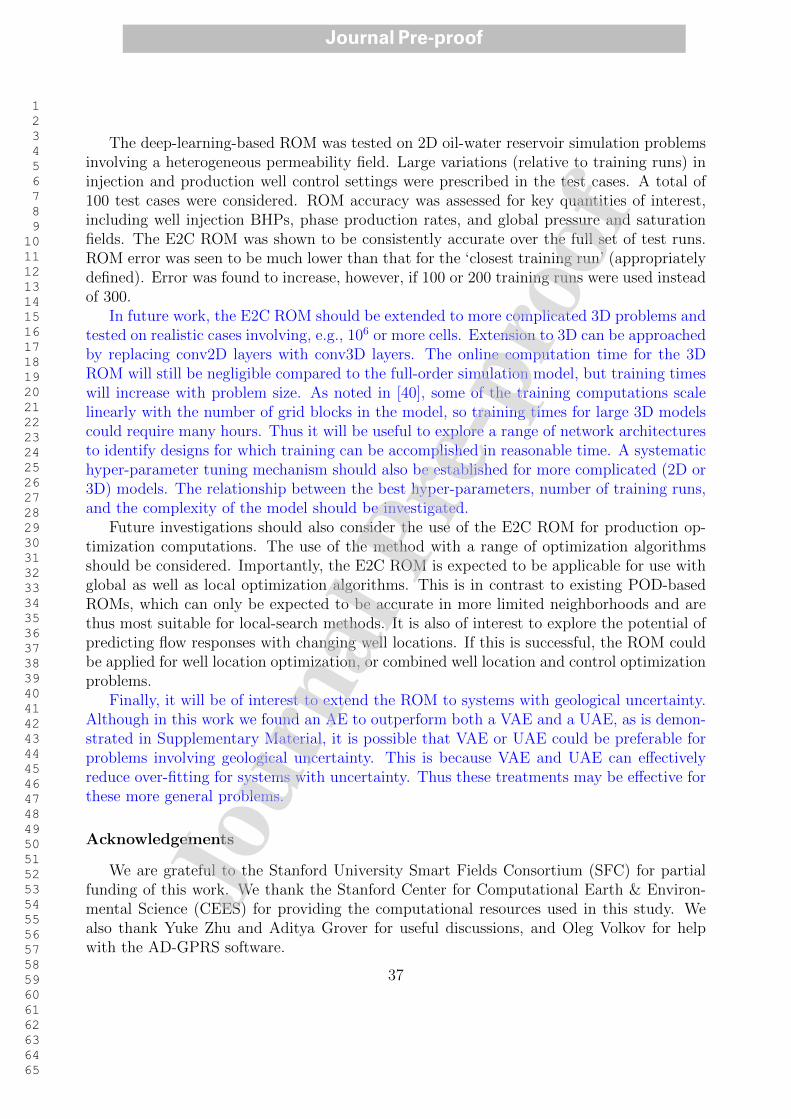
1

2

3

4

5

6

7

8

9

10

11

12

13

14

15

16

17

18

19

20

21

22

23

24

25

26

27

28

29

30

31

32

33

34

35

36

37

38

39

40

41

42

43

44

45

46

47

48

49

50

51

52

53

54

55

56

57

58

59

60

61

62

63

64

65

The deep-learning-based ROM was tested on 2D oil-water reservoir simulation problemsinvolving a heterogeneous permeability field. Large variations (relative to training runs) ininjection and production well control settings were prescribed in the test cases. A total of100 test cases were considered. ROM accuracy was assessed for key quantities of interest,including well injection BHPs, phase production rates, and global pressure and saturationfields. The E2C ROM was shown to be consistently accurate over the full set of test runs.ROM error was seen to be much lower than that for the ‘closest training run’ (appropriatelydefined). Error was found to increase, however, if 100 or 200 training runs were used insteadof 300.

In future work, the E2C ROM should be extended to more complicated 3D problems andtested on realistic cases involving, e.g., 106 or more cells. Extension to 3D can be approachedby replacing conv2D layers with conv3D layers. The online computation time for the 3DROM will still be negligible compared to the full-order simulation model, but training timeswill increase with problem size. As noted in [40], some of the training computations scalelinearly with the number of grid blocks in the model, so training times for large 3D modelscould require many hours. Thus it will be useful to explore a range of network architecturesto identify designs for which training can be accomplished in reasonable time. A systematichyper-parameter tuning mechanism should also be established for more complicated (2D or3D) models. The relationship between the best hyper-parameters, number of training runs,and the complexity of the model should be investigated.

Future investigations should also consider the use of the E2C ROM for production op-timization computations. The use of the method with a range of optimization algorithmsshould be considered. Importantly, the E2C ROM is expected to be applicable for use withglobal as well as local optimization algorithms. This is in contrast to existing POD-basedROMs, which can only be expected to be accurate in more limited neighborhoods and arethus most suitable for local-search methods. It is also of interest to explore the potential ofpredicting flow responses with changing well locations. If this is successful, the ROM couldbe applied for well location optimization, or combined well location and control optimizationproblems.

Finally, it will be of interest to extend the ROM to systems with geological uncertainty.Although in this work we found an AE to outperform both a VAE and a UAE, as is demon-strated in Supplementary Material, it is possible that VAE or UAE could be preferable forproblems involving geological uncertainty. This is because VAE and UAE can effectivelyreduce over-fitting for systems with uncertainty. Thus these treatments may be effective forthese more general problems.

Acknowledgements

We are grateful to the Stanford University Smart Fields Consortium (SFC) for partialfunding of this work. We thank the Stanford Center for Computational Earth & Environ-mental Science (CEES) for providing the computational resources used in this study. Wealso thank Yuke Zhu and Aditya Grover for useful discussions, and Oleg Volkov for helpwith the AD-GPRS software.

37

Jour

nal P

re-p

roof

Journal Pre-proof

1

2

3

4

5

6

7

8

9

10

11

12

13

14

15

16

17

18

19

20

21

22

23

24

25

26

27

28

29

30

31

32

33

34

35

36

37

38

39

40

41

42

43

44

45

46

47

48

49

50

51

52

53

54

55

56

57

58

59

60

61

62

63

64

65

References

[1] K. Carlberg, C. Bou-Mosleh, C. Farhat, Efficient non-linear model reduction via a least-squares Petrov–Galerkin projection and compressive tensor approximations, International Journal for Numerical Meth-ods in Engineering 86 (2) (2011) 155–181.

[2] M. J. Zahr, P. Avery, C. Farhat, A multilevel projection-based model order reduction framework fornonlinear dynamic multiscale problems in structural and solid mechanics, International Journal forNumerical Methods in Engineering 112 (8) (2017) 855–881.

[3] D. Amsallem, M. J. Zahr, C. Farhat, Nonlinear model order reduction based on local reduced-orderbases, International Journal for Numerical Methods in Engineering 92 (10) (2012) 891–916.

[4] K. Carlberg, C. Farhat, J. Cortial, D. Amsallem, The GNAT method for nonlinear model reduction:effective implementation and application to computational fluid dynamics and turbulent flows, Journalof Computational Physics 242 (2013) 623–647.

[5] S. Chaturantabut, D. C. Sorensen, Nonlinear model reduction via discrete empirical interpolation,SIAM Journal on Scientific Computing 32 (5) (2010) 2737–2764.

[6] S. Yoon, Z. M. Alghareeb, J. R. Williams, Hyper-reduced-order models for subsurface flow simulation,SPE Journal 21 (06) (2016) 2128–2140.

[7] Y. Yang, M. Ghasemi, E. Gildin, Y. Efendiev, V. Calo, Fast multiscale reservoir simulations withPOD-DEIM model reduction, SPE Journal 21 (06) (2016) 2141–2154.

[8] Y. Efendiev, E. Gildin, Y. Yang, Online adaptive local-global model reduction for flows in heterogeneousporous media, Computation 4 (2) (2016) 22.

[9] X. Tan, E. Gildin, H. Florez, S. Trehan, Y. Yang, N. Hoda, Trajectory-based DEIM (TDEIM) modelreduction applied to reservoir simulation, Computational Geosciences 23 (1) (2019) 35–53.

[10] R. Jiang, L. J. Durlofsky, Implementation and detailed assessment of a GNAT reduced-order model forsubsurface flow simulation, Journal of Computational Physics 379 (2019) 192–213.

[11] H. Florez, E. Gildin, Model-order reduction of coupled flow and geomechanics in ultra-low permeabilityULP reservoirs (SPE paper 193911), in: SPE Reservoir Simulation Conference, Galveston, Texas, USA,2019.

[12] D. Xiao, F. Fang, C. Pain, G. Hu, Non-intrusive reduced-order modelling of the Navier–Stokes equationsbased on RBF interpolation, International Journal for Numerical Methods in Fluids 79 (11) (2015) 580–595.

[13] W. Kostorz, A. Muggeridge, M. Jackson, A. Moncorge, Non-intrusive reduced order modelling for re-construction of saturation distributions (SPE paper 193831), in: SPE Reservoir Simulation Conference,Galveston, Texas, USA, 2019.

[14] M. Rewienski, J. White, A trajectory piecewise-linear approach to model order reduction and fastsimulation of nonlinear circuits and micromachined devices, IEEE Transactions on Computer-aidedDesign of Integrated Circuits and Systems 22 (2) (2003) 155–170.

[15] M. Cardoso, L. J. Durlofsky, Linearized reduced-order models for subsurface flow simulation, Journalof Computational Physics 229 (3) (2010) 681–700.

[16] J. He, J. Sætrom, L. J. Durlofsky, Enhanced linearized reduced-order models for subsurface flow simu-lation, Journal of Computational Physics 230 (23) (2011) 8313–8341.

[17] J. He, L. J. Durlofsky, Reduced-order modeling for compositional simulation by use of trajectorypiecewise linearization, SPE Journal 19 (05) (2014) 858–872.

[18] J. He, L. J. Durlofsky, Constraint reduction procedures for reduced-order subsurface flow models basedon POD-TPWL, International Journal for Numerical Methods in Engineering 103 (1) (2015) 1–30.

[19] Z. L. Jin, L. J. Durlofsky, Reduced-order modeling of CO2 storage operations, International Journal ofGreenhouse Gas Control 68 (2018) 49–67.

[20] Z. L. Jin, T. Garipov, O. Volkov, L. J. Durlofsky, Reduced-order modeling of coupled flow-geomechanicsproblems (SPE paper 193863), in: SPE Reservoir Simulation Conference, Galveston, Texas, USA, 2019.

[21] S. Trehan, L. J. Durlofsky, Trajectory piecewise quadratic reduced-order model for subsurface flow, withapplication to PDE-constrained optimization, Journal of Computational Physics 326 (2016) 446–473.

[22] K. Lee, J. Lim, S. Ahn, J. Kim, Feature extraction using a deep learning algorithm for uncertainty

38

Jour

nal P

re-p

roof

Journal Pre-proof

1

2

3

4

5

6

7

8

9

10

11

12

13

14

15

16

17

18

19

20

21

22

23

24

25

26

27

28

29

30

31

32

33

34

35

36

37

38

39

40

41

42

43

44

45

46

47

48

49

50

51

52

53

54

55

56

57

58

59

60

61

62

63

64

65

quantification of channelized reservoirs, Journal of Petroleum Science and Engineering 171 (2018) 1007–1022.

[23] S. W. Canchumuni, A. A. Emerick, M. A. C. Pacheco, History matching geological facies models basedon ensemble smoother and deep generative models, Journal of Petroleum Science and Engineering 177(2019) 941–958.

[24] D. P. Kingma, M. Welling, Auto-encoding variational Bayes, arXiv preprint arXiv:1312.6114 .[25] E. Laloy, R. Herault, D. Jacques, N. Linde, Training-image based geostatistical inversion using a spatial

generative adversarial neural network, Water Resources Research 54 (1) (2018) 381–406.[26] Y. Liu, W. Sun, L. J. Durlofsky, A deep-learning-based geological parameterization for history matching

complex models, Mathematical Geosciences 51 (2019) 725–766.[27] Y. Liu, L. J. Durlofsky, Multilevel strategies and geological parameterizations for history matching

complex reservoir models (SPE paper 193895), in: SPE Reservoir Simulation Conference, Galveston,Texas, USA, 2019.

[28] J. Johnson, A. Alahi, F.-F. Li, Perceptual losses for real-time style transfer and super-resolution, in:European Conference on Computer Vision, Amsterdam, The Netherlands, 2016.

[29] Y. Zhu, N. Zabaras, Bayesian deep convolutional encoder–decoder networks for surrogate modeling anduncertainty quantification, Journal of Computational Physics 366 (2018) 415–447.

[30] S. Mo, Y. Zhu, N. Zabaras, X. Shi, J. Wu, Deep convolutional encoder-decoder networks for uncertaintyquantification of dynamic multiphase flow in heterogeneous media, Water Resources Research 55 (1)(2019) 703–728.

[31] K. Lee, K. T. Carlberg, Model reduction of dynamical systems on nonlinear manifolds using deepconvolutional autoencoders, Journal of Computational Physics 404 (2020) 108973.

[32] J. N. Kani, A. H. Elsheikh, Reduced-order modeling of subsurface multi-phase flow models using deepresidual recurrent neural networks, Transport in Porous Media 126 (3) (2019) 713–741.

[33] J. Zhang, S. W. Cheung, Y. Efendiev, E. Gildin, E. T. Chung, Deep model reduction-model learning forreservoir simulation (SPE paper 193912), in: SPE Reservoir Simulation Conference, Galveston, Texas,USA, 2019.

[34] Z. Wang, D. Xiao, F. Fang, R. Govindan, C. C. Pain, Y. Guo, Model identification of reduced orderfluid dynamics systems using deep learning, International Journal for Numerical Methods in Fluids86 (4) (2018) 255–268.

[35] F. A. Gers, J. Schmidhuber, F. Cummins, Learning to forget: continual prediction with LSTM, in: 9thInternational Conference on Artificial Neural Networks, Edinburgh, UK, 1999.

[36] F. J. Gonzalez, M. Balajewicz, Deep convolutional recurrent autoencoders for learning low-dimensionalfeature dynamics of fluid systems, arXiv preprint arXiv:1808.01346 .

[37] P. Temirchev, M. Simonov, R. Kostoev, E. Burnaev, I. Oseledets, A. Akhmetov, A. Margarit, A. Sit-nikov, D. Koroteev, Deep neural networks predicting oil movement in a development unit, Journal ofPetroleum Science and Engineering 184 (2020) 106513.

[38] J. Chung, C. Gulcehre, K. Cho, Y. Bengio, Empirical evaluation of gated recurrent neural networks onsequence modeling, arXiv preprint arXiv:1412.3555 .

[39] P. Temirchev, A. Gubanova, R. Kostoev, A. Gryzlov, D. Voloskov, D. Koroteev, M. Simonov, A. Akhme-tov, A. Margarit, A. Ershov, Reduced order reservoir simulation with neural-network based hybridmodel (SPE paper 196864), in: SPE Russian Petroleum Technology Conference, Moscow, Russia,2019.

[40] M. Tang, Y. Liu, L. J. Durlofsky, A deep-learning-based surrogate model for data assimilation indynamic subsurface flow problems, arXiv preprint arXiv:1908.05823 .

[41] M. Raissi, P. Perdikaris, G. Karniadakis, Physics-informed neural networks: a deep learning frameworkfor solving forward and inverse problems involving nonlinear partial differential equations, Journal ofComputational Physics 378 (2019) 686–707.

[42] Y. Zhu, N. Zabaras, P.-S. Koutsourelakis, P. Perdikaris, Physics-constrained deep learning for high-dimensional surrogate modeling and uncertainty quantification without labeled data, Journal of Com-putational Physics 394 (2019) 56–81.

39

Jour

nal P

re-p

roof

Journal Pre-proof

1

2

3

4

5

6

7

8

9

10

11

12

13

14

15

16

17

18

19

20

21

22

23

24

25

26

27

28

29

30

31

32

33

34

35

36

37

38

39

40

41

42

43

44

45

46

47

48

49

50

51

52

53

54

55

56

57

58

59

60

61

62

63

64

65

[43] D. P. Kingma, P. Dhariwal, Glow: generative flow with invertible 1x1 convolutions, in: Advances inNeural Information Processing Systems, Montreal, Canada, 2018.

[44] M. Watter, J. Springenberg, J. Boedecker, M. Riedmiller, Embed to control: A locally linear latentdynamics model for control from raw images, in: Advances in Neural Information Processing Systems,Montreal, Canada, 2015.

[45] A. Grover, S. Ermon, Uncertainty autoencoders: learning compressed representations via variationalinformation maximization, arXiv preprint arXiv:1812.10539 .

[46] Y. Zhou, Parallel General-Purpose Reservoir Simulation with Coupled Reservoir Models and Multiseg-ment Wells, Ph.D. thesis, Stanford University, 2012.

[47] O. Ronneberger, P. Fischer, T. Brox, U-net: Convolutional networks for biomedical image segmenta-tion, in: International Conference on Medical Image Computing and Computer-Assisted Intervention,Munich, Germany, 2015.

[48] D. Eigen, C. Puhrsch, R. Fergus, Depth map prediction from a single image using a multi-scale deepnetwork, in: Advances in Neural Information Processing Systems, Montreal, Canada, 2366–2374, 2014.

[49] Y. LeCun, L. Bottou, Y. Bengio, P. Haffner, Gradient-based learning applied to document recognition,Proceedings of the IEEE 86 (11) (1998) 2278–2324.

[50] S. Ioffe, C. Szegedy, Batch normalization: Accelerating deep network training by reducing internalcovariate shift, arXiv preprint arXiv:1502.03167 .

[51] X. Glorot, A. Bordes, Y. Bengio, Deep sparse rectifier neural networks, in: Fourteenth InternationalConference on Artificial Intelligence and Statistics, Ft. Lauderdale, Florida, USA, 2011.

[52] X. Glorot, Y. Bengio, Understanding the difficulty of training deep feedforward neural networks, in:Thirteenth International Conference on Artificial Intelligence and Statistics, Sardinia, Italy, 2010.

[53] K. He, X. Zhang, S. Ren, J. Sun, Deep residual learning for image recognition, in: IEEE Conferenceon Computer Vision and Pattern Recognition, Las Vegas, Nevada, USA, 2016.

[54] G. Huang, Z. Liu, L. Van Der Maaten, K. Q. Weinberger, Densely connected convolutional networks,in: Computer Vision and Pattern Recognition, Honolulu, USA, 2017.

[55] D. W. Peaceman, Interpretation of well-block pressures in numerical reservoir simulation, SPE Journal18 (03) (1978) 183–194.

[56] D. P. Kingma, J. Ba, Adam: A method for stochastic optimization, arXiv preprint arXiv:1412.6980 .[57] F. Chollet, et al., Keras, https://github.com/fchollet/keras, 2015.[58] M. Abadi, et al., TensorFlow: large-scale machine learning on heterogeneous systems,

https://www.tensorflow.org/, 2015.

40

Jour

nal P

re-p

roof

Journal Pre-proof

• Reduced-order model for subsurface flow based on embed-to-control (E2C) developed

• Direct analogies between E2C ROM and existing POD-TPWL ROM are provided

• Accuracy of E2C ROM is improved by adding a physics-based loss function

• E2C ROM assessed on test cases with large variations in control parameters

• Reliable predictions achieved for global quantities and well responses

*Highlights

Jour

nal P

re-p

roof

Journal Pre-proof

Declaration of interests

☒ The authors declare that they have no known competing financial interests or personal relationships

that could have appeared to influence the work reported in this paper.

☐The authors declare the following financial interests/personal relationships which may be considered

as potential competing interests:

*Declaration of Interest Statement

Jour

nal P

re-p

roof

Journal Pre-proof

CRediT author statement

Zhaoyang Larry Jin: Conceptualization, Methodology, Data curation,

Software, Investigation, Formal analysis, Visualization, Validation,

Writing- Original draft preparation, Writing- Reviewing and Editing.

Yimin Liu: Methodology, Software, Writing- Reviewing and Editing.

Louis J. Durlofsky: Supervision, Project administration, Funding

acquisition, Writing- Reviewing and Editing.

*Credit Author Statement

Jour

nal P

re-p

roof

Journal Pre-proof