Deep ADMM-Net for Compressive Sensing MRI

Yan YangXi’an Jiaotong University

yangyan92@stu.xjtu.edu.cn

Jian SunXi’an Jiaotong University

jiansun@mail.xjtu.edu.cn

Huibin LiXi’an Jiaotong University

huibinli@mail.xjtu.edu.cn

Zongben XuXi’an Jiaotong Universityzbxu@mail.xjtu.edu.cn

Abstract

Compressive Sensing (CS) is an effective approach for fast Magnetic ResonanceImaging (MRI). It aims at reconstructing MR image from a small number of under-sampled data in k-space, and accelerating the data acquisition in MRI. To improvethe current MRI system in reconstruction accuracy and computational speed, inthis paper, we propose a novel deep architecture, dubbed ADMM-Net. ADMM-Net is defined over a data flow graph, which is derived from the iterative pro-cedures in Alternating Direction Method of Multipliers (ADMM) algorithm foroptimizing a CS-based MRI model. In the training phase, all parameters of thenet, e.g., image transforms, shrinkage functions, etc., are discriminatively trainedend-to-end using L-BFGS algorithm. In the testing phase, it has computationaloverhead similar to ADMM but uses optimized parameters learned from the train-ing data for CS-based reconstruction task. Experiments on MRI image reconstruc-tion under different sampling ratios in k-space demonstrate that it significantlyimproves the baseline ADMM algorithm and achieves high reconstruction accura-cies with fast computational speed.

1 Introduction

Magnetic Resonance Imaging (MRI) is a non-invasive imaging technique providing both functionaland anatomical information for clinical diagnosis. Imaging speed is a fundamental challenge. FastMRI techniques are essentially demanded for accelerating data acquisition while still reconstructinghigh quality image. Compressive sensing MRI (CS-MRI) is an effective approach allowing for datasampling rate much lower than Nyquist rate without significantly degrading the image quality [1].

CS-MRI methods first sample data in k-space (i.e., Fourier space), then reconstruct image usingcompressive sensing theory. Regularization related to the data prior is a key component in a CS-MRI model to reduce imaging artifacts and improve imaging precision. Sparse regularization can beexplored in specific transform domain or general dictionary-based subspace [2]. Total Variation (TV)regularization in gradient domain has been widely utilized in MRI [3, 4]. Although it is easy andfast to optimize, it introduces staircase artifacts in reconstructed image. Methods in [5, 6] leveragesparse regularization in the wavelet domain. Dictionary learning methods rely on a dictionary oflocal patches to improve the reconstruction accuracy [7, 8]. The non-local method uses groups ofsimilar local patches for joint patch-level reconstruction to better preserve image details [9, 10, 11].In performance, the basic CS-MRI methods run fast but produce less accurate reconstruction results.The non-local and dictionary learning-based methods generally output higher quality MR images,but suffer from slow reconstruction speed. In a CS-MRI model, it is commonly challenging tochoose an optimal image transform domain / subspace and the corresponding sparse regularization.

30th Conference on Neural Information Processing Systems (NIPS 2016), Barcelona, Spain.

To optimize the CS-MRI models, Alternating Direction Method of Multipliers (ADMM) has provento be an efficient variable splitting algorithm with convergence guarantee [4, 12, 13]. It considersthe augmented Lagrangian function of a given CS-MRI model, and splits variables into subgroups,which can be alternatively optimized by solving a few simply subproblems. Although ADMM isgenerally efficient, it is not trivial to determine the optimal parameters (e.g., update rates, penaltyparameters) influencing accuracy in CS-MRI.

In this work, we aim to design a fast yet accurate method to reconstruct high-quality MR imagesfrom under-sampled k-space data. We propose a novel deep architecture, dubbed ADMM-Net, in-spired by the ADMM iterative procedures for optimizing a general CS-MRI model. This deep archi-tecture consists of multiple stages, each of which corresponds to an iteration in ADMM algorithm.More specifically, we define a deep architecture represented by a data flow graph [14] for ADMMprocedures. The operations in ADMM are represented as graph nodes, and the data flow betweentwo operations in ADMM is represented by a directed edge. Therefore, the ADMM iterative proce-dures naturally determine a deep architecture over a data flow graph. Given an under-sampled datain k-space, it flows over the graph and generates a reconstructed image. All the parameters (e.g.,transforms, shrinkage functions, penalty parameters, etc.) in the deep architecture can be discrimi-natively learned from training pairs of under-sampled data in k-space and reconstructed image usingfully sampled data by backpropagation [15] over the data flow graph.

Our experiments demonstrate that the proposed deep ADMM-Net is effective both in reconstruc-tion accuracy and speed. Compared with the baseline methods using sparse regularization in trans-form domain, it achieves significantly higher accuracy and takes comparable computational time.Compared with the state-of-the-art methods using dictionary learning and non-local techniques, itachieves high accuracy in significantly faster computational speed.

The main contributions of this paper can be summarized as follows. We propose a novel deepADMM-Net by reformulating an ADMM algorithm to a deep network for CS-MRI. This is achievedby designing a data flow graph for ADMM to effectively build and train the ADMM-Net. ADMM-Net achieves high accuracy in MR image reconstruction with fast computational speed justified inexperiments. The discriminative parameter learning approach has been applied to sparse codingand Markov Random Filed [16, 17, 18, 19]. But, to the best of our knowledge, this is the firstcomputational framework that maps an ADMM algorithm to a learnable deep architecture.

2 Deep ADMM-Net for Fast MRI

2.1 Compressive Sensing MRI Model and ADMM Algorithm

General CS-MRI Model: Assume x ∈ CN is an MRI image to be reconstructed, y ∈ CN ′(N ′ <

N ) is the under-sampled k-space data, according to the CS theory, the reconstructed image can beestimated by solving the following optimization problem:

x̂ = argminx

{1

2∥Ax− y∥22 +

L∑l=1

λlg(Dlx)

}, (1)

where A = PF ∈ RN ′×N is a measurement matrix, P ∈ RN ′×N is a under-sampling matrix, and Fis a Fourier transform. Dl denotes a transform matrix for a filtering operation, e.g., Discrete WaveletTransform (DWT), Discrete Cosine Transform (DCT), etc. g(·) is a regularization function derivedfrom the data prior, e.g., lq-norm (0 ≤ q ≤ 1) for a sparse prior. λl is a regularization parameter.

ADMM solver: [12] The above optimization problem can be solved efficiently using ADMM algo-rithm. By introducing auxiliary variables z = {z1, z2, · · · , zL}, Eqn. (1) is equivalent to:

minx,z

1

2∥Ax− y∥22 +

L∑l=1

λlg(zl) s.t. zl = Dlx, ∀ l ∈ [1, 2, · · · , L]. (2)

Its augmented Lagrangian function is :

Lρ(x, z, α) =1

2∥Ax− y∥22 +

L∑l=1

λlg(zl)−L∑

l=1

⟨αl, zl −Dlx⟩+L∑

l=1

ρl2∥zl −Dlx∥22, (3)

2

Sampling datain k-space

ReconstructedMR image

stage n

(1)X

(n-1)C (n-1)

Z (n)X

(n-1)M

(n)C (n)

Z(n+1)

X

(n)M

(n+1)C

(n+1)Z s 1(N )

X

(n+1)M

(n-1)X

Figure 1: The data flow graph for the ADMM optimization of a general CS-MRI model. This graphconsists of four types of nodes: reconstruction (X), convolution (C), non-linear transform (Z), andmultiplier update (M). An under-sampled data in k-space is successively processed over the graph,and finally generates a MR image. Our deep ADMM-Net is defined over this data flow graph.

where α = {αl} are Lagrangian multipliers and ρ = {ρl} are penalty parameters. ADMM alterna-tively optimizes {x, z, α} by solving the following three subproblems:

x(n+1) = argminx

12∥Ax− y∥22 −

∑Ll=1⟨α

(n)l , z

(n)l −Dlx⟩+

∑Ll=1

ρl

2 ∥z(n)l −Dlx∥22,

z(n+1) = argminz

∑Ll=1 λlg(zl)−

∑Ll=1⟨α

(n)l , zl −Dlx

(n+1)⟩+∑L

l=1ρl

2 ∥zl −Dlx(n+1)∥22,

α(n+1) = argminα

∑Ll=1⟨αl, Dlx

(n+1) − z(n+1)l ⟩,

(4)where n ∈ [1, 2, · · · , Ns] denotes n-th iteration. For simplicity, let βl =

αl

ρl(l ∈ [1, 2, · · · , L]), and

substitute A = PF into Eqn. (4). Then the three subproblems have the following solutions:X(n) : x(n) = FT [PTP +

∑Ll=1 ρlFDT

l DlFT ]−1[PT y +

∑Ll=1 ρlFDT

l (z(n−1)l − β

(n−1)l )],

Z(n) : z(n)l = S(Dlx

(n) + β(n−1)l ;λl/ρl),

M(n) : β(n)l = β

(n−1)l + ηl(Dlx

(n) − z(n)l ),

(5)where x(n) can be efficiently computed by fast Fourier transform, S(·) is a nonlinear shrinkagefunction. It is usually a soft or hard thresholding function corresponding to the sparse regularizationof l1-norm and l0-norm respectively [20]. The parameter ηl is an update rate.

In CS-MRI, it commonly needs to run the ADMM algorithm in dozens of iterations to get a satis-factory reconstruction result. However, it is challenging to choose the transform Dl and shrinkagefunction S(·) for general regularization function g(·). Moreover, it is also not trivial to tune theparameters ρl and ηl for k-space data with different sampling ratios. To overcome these difficul-ties, we will design a data flow graph for the ADMM algorithm, over which we can define a deepADMM-Net to discriminatively learn all the above transforms, functions, and parameters.

2.2 Data Flow Graph for the ADMM Algorithm

To design our deep ADMM-Net, we first map the ADMM iterative procedures in Eqn. (5) to adata flow graph [14]. As shown in Fig. 1, this graph comprises of nodes corresponding to differentoperations in ADMM, and directed edges corresponding to the data flows between operations. Inthis case, the n-th iteration of ADMM algorithm corresponds to the n-th stage of the data flow graph.In the n-th stage of the graph, there are four types of nodes mapped from four types of operations inADMM, i.e., reconstruction operation (X(n)), convolution operation (C(n)) defined by {Dlx

(n)}Ll=1,nonlinear transform operation (Z(n)) defined by S(·), and multiplier update operation (M(n)) inEqn. (5). The whole data flow graph is a multiple repetition of the above stages corresponding tosuccessive iterations in ADMM. Given an under-sampled data in k-space, it flows over the graphand finally generates a reconstructed image. In this way, we map the ADMM iterations to a dataflow graph, which is useful to define and train our deep ADMM-Net in the following sections.

2.3 Deep ADMM-Net

Our deep ADMM-Net is defined over the data flow graph. It keeps the graph structure but generalizesthe four types of operations to have learnable parameters as network layers. These operations arenow generalized as reconstruction layer, convolution layer, non-linear transform layer, and multiplierupdate layer. We next discuss them in details.

3

Reconstruction layer (X(n)): This layer reconstructs an MRI image following the reconstructionoperation X(n) in Eqn. (5). Given z

(n−1)l and β

(n−1)l , the output of this layer is defined as:

x(n) = FT (PTP +L∑

l=1

ρ(n)l FH

(n)l

TH(n)l FT )−1[PT y+

L∑l=1

ρ(n)l FH

(n)l

T (z(n−1)l −β

(n−1)l )], (6)

where H(n)l is the l-th filter, ρ(n)l is the l-th penalty parameter, l = 1, · · · , L, and y is the input

under-sampled data in k-space. In the first stage (n = 1), z(0)l and β(0)l are initialized to zeros,

therefore x(1) = FT (PTP +∑L

l=1 ρ(1)l FH

(1)l

TH(1)l FT )−1(PT y).

Convolution layer (C(n)): It performs convolution operation to transform an image into trans-form domain. Given an image x(n), i.e., a reconstructed image in stage n, the output is

c(n)l = D

(n)l x(n), (7)

where D(n)l is a learnable filter matrix in stage n. Different from the original ADMM, we do not

constrain the filters D(n)l and H

(n)l to be the same to increase the network capacity.

Nonlinear transform layer (Z(n)): This layer performs nonlinear transform inspired by theshrinkage function S(·) defined in Z(n) in Eqn. (5). Instead of setting it to be a shrinkage func-tion determined by the regularization term g(·) in Eqn. (1), we aim to learn more general functionusing piecewise linear function. Given c

(n)l and β

(n−1)l , the output of this layer is defined as:

z(n)l = SPLF (c

(n)l + β

(n−1)l ; {pi, q(n)l,i }

Nci=1), (8)

where SPLF (·) is a piecewise linear function determined by a set of control points {pi, q(n)l,i }Nci=1. i.e.

SPLF (a; {pi, q(n)l,i }Nci=1) =

a+ q

(n)l,1 − p1, a < p1,

a+ q(n)l,Nc

− pNc , a > pNc ,

q(n)l,k +

(a−pk)(q(n)l,k+1−q

(n)l,k )

pk+1−pk, p1 ≤ a ≤ pNc ,

(9)

where k = ⌊ a−p1

p2−p1⌋, {pi}Nc

i=1 are predefined positions uniformly located within [-1,1], and {q(n)l,i }Nci=1

are the values at these positions for l-th filter in n-th stage. Figure 2 gives an illustrative example.Since a piecewise linear function can approximate any function, we can learn flexible nonlineartransform function from data beyond the off-the-shelf hard or soft thresholding functions.

(𝑝𝑖,𝑞𝑙,𝑖(𝑛)

)

… …-1 1

Figure 2: Illustration of a piecewise linear function determined by a set of control points.

Multiplier update layer (M(n)): This layer is defined by the Lagrangian multiplier updatingprocedure M(n) in Eqn. (5). The output of this layer in stage n is defined as:

β(n)l = β

(n−1)l + η

(n)l (c

(n)l − z

(n)l ), (10)

where η(n)l are learnable parameters.

Network Parameters: These layers are organized in a data flow graph shown in Fig. 1. In thedeep architecture, we aim to learn the following parameters: H(n)

l and ρ(n)l in reconstruction layer,

filters D(n)l in convolution layer, {q(n)l,i }

Nci=1 in nonlinear transform layer, η(n)l in multiplier update

layer, where l ∈ [1, 2, · · · , L] and n ∈ [1, 2, · · · , Ns] are the indexes for the filters and stagesrespectively. All of these parameters are taken as the network parameters to be learned.

Figure 3 shows an example of a deep ADMM-Net with three stages. The under-sampled data ink-space flows over three stages in a order from circled number 1 to number 12, followed by afinal reconstruction layer with circled number 13 and generates a reconstructed image. Immediatereconstruction result at each stage is shown under each reconstruction layer.

4

①

④

(1)X

②

(1)C

③

(1)Z

⑤

(2)X

(1)M ⑧

⑥

(2)C

⑦

(2)Z

⑨

(3)X

(2)M ⑫

⑩

(3)C

⑪

(3)Z

⑬

(4)X

(3)MSampling data

in k-spaceReconstructed

MR image

Figure 3: An example of deep ADMM-Net with three stages. The sampled data in k-space issuccessively processed by operations in a order from 1 to 12, followed by a reconstruction layerX(4) to output the final reconstructed image. The reconstructed image in each stage is shown undereach reconstruction layer.

3 Network Training

We take the reconstructed MR image using fully sampled data in k-space as the ground-truth MRimage xgt, and under-sampled data y in k-space as the input. Then a training set Γ is constructedcontaining pairs of under-sampled data and ground-truth MR image. We choose normalized meansquare error (NMSE) as the loss function in network training. Given pairs of training data, the lossbetween the network output and ground truth is defined as:

E(Θ) =1

|Γ|∑

(y,xgt)∈Γ

√∥x̂(y,Θ)− xgt∥22√

∥xgt∥22, (11)

where x̂(y,Θ) is the network output based on network parameter Θ and under-sampled data y in k-space. We learn the parameters Θ = {(q(n)l,i )

Nci=1, D

(n)l , H

(n)l , ρ

(n)l , η

(n)l }Ns

n=1 ∪ {H(Ns+1)l , ρ

(Ns+1)l }

(l = 1, · · · , L) by minimizing the loss w.r.t. them using L-BFGS1. In the following, we first discussthe initialization of these parameters and then compute the gradients of the loss function E(Θ) w.r.t.parameters Θ using backpropagation (BP) [21] over the data flow graph.

3.1 Initialization

We initialize the network parameters Θ according to the ADMM solver of the following baselineCS-MRI model:

argminx

{1

2∥Ax− y∥22 + λ

L∑l=1

||Dlx||1

}. (12)

In this model, we set Dl as a DCT basis and impose l1-norm regularization in the DCT trans-form space. The function S(·) in ADMM algorithm (Eqn. (5)) is a soft thresholding function:S(t;λ/ρl) = sgn(t)(|t| − λ/ρl) when |t| > λ/ρl, and 0 otherwise. For each n-th stage of deepADMM-Net, filters D(n)

l in convolution layers and H(n)l in reconstruction layers are initialized to be

Dl in Eqn. (12). In the nonlinear transform layer, we uniformly choose 101 positions located within[-1,1], and each value q

(n)l,i is initialized as S(pi;λ/ρl). Parameters λ, ρ

(n)l , η

(n)l are initialized to

be the corresponding values in the ADMM algorithm. In this case, the initialized net is exactly arealization of ADMM optimizing Eqn. (12), therefore outputs the same reconstructed image as theADMM algorithm. The optimization of the network parameters is expected to produce improvedreconstruction result.

3.2 Gradient Computation by Backpropagation over Data Flow Graph

It is challenging to compute the gradients of loss w.r.t. parameters using backpropagation over thedeep architecture in Fig. 1, because it is a directed graph. In the forward pass, we process the dataof n-th stage in the order of X(n),C(n),Z(n) and M(n). In the backward pass, the gradients are

1http://users.eecs.northwestern.edu/~nocedal/lbfgsb.html

5

( )n

lc(n)

Z ( 1)nx

(b) Non-linear transform layer

( )n

l

(c) Convolution layer

( )nx(n)

C( )n

lz

( )n

l

( )n

lz

( 1)n

l

(n)M

( 1)n

lz

(a) Multiplier update layer

( 1)n

l

(d) Reconstruction layer

(n)X

( )n

lc

( )n

lc

( )n

l

( )nl

( )nl

( 1)nl ( )n

lz

( 1)n

lz ( )n

lc

()n

lc

( )nx

(1)

nl

( 1)nx

()n

lz

Figure 4: Illustration of four types of graph nodes (i.e., layers in network) and their data flows instage n. The solid arrow indicates the data flow in forward pass and dashed arrow indicates thebackward pass when computing gradients in backpropagation.

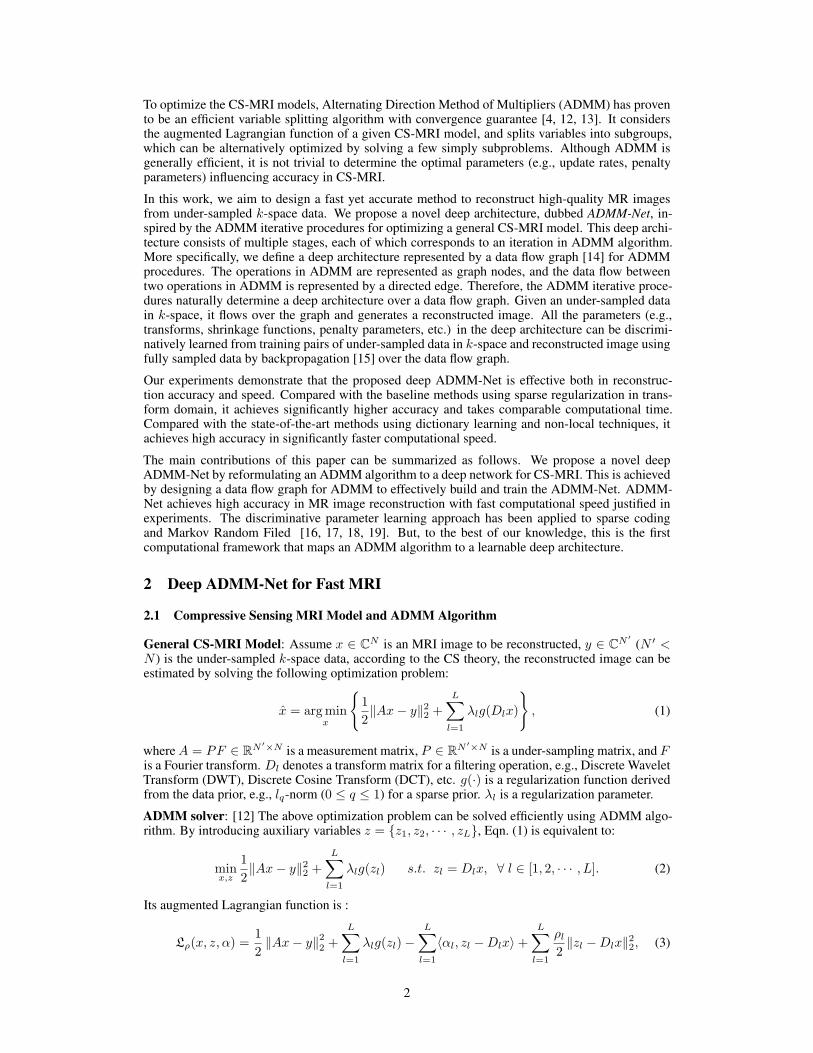
computed in an inverse order. Figure 3 shows an example, where the gradient can be computedbackwardly from the layers with circled number 13 to 1 successively. For a stage n, Fig. 4 showsfour types of nodes (i.e., network layers) and the data flow over them. Each node has multiple inputsand (or) outputs. We next briefly introduce the gradients computation for each layer in a typicalstage n (n < Ns). Please refer to supplementary material for details.

Multiplier update layer (M(n)): As shown in Fig. 4(a), this layer has three sets of inputs:{β(n−1)

l }, {c(n)l } and {z(n)l }. Its output {β(n)l } is the input to compute {β(n+1)

l }, {z(n+1)l } and

x(n+1). The parameters of this layer are η(n)l , l = 1, · · · , L. The gradients of loss w.r.t. the parame-

ters can be computed as:

∂E

∂η(n)l

=∂E

∂β(n)l

∂β(n)l

∂η(n)l

, where∂E

∂β(n)l

=∂E

∂β(n+1)l

∂β(n+1)l

∂β(n)l

+∂E

∂z(n+1)l

∂z(n+1)l

∂β(n)l

+∂E

∂x(n+1)

∂x(n+1)

∂β(n)l

.

∂E

∂β(n)l

is the summation of gradients along the three dashed blue arrows in Fig. 4(a). We also compute

gradients of the output in this layer w.r.t. its inputs: ∂β(n)l

∂β(n−1)l

,∂β(n)l

∂c(n)l

, and ∂β(n)l

∂z(n)l

.

Nonlinear transform layer (Z(n)): As shown in Fig. 4(b), this layer has two sets of inputs:{β(n−1)

l }, {c(n)l }, and its output {z(n)l } is the input for computing {β(n)l } and x(n+1) in next stage.

The parameters of this layers are {q(n)l,i }Nci=1, l = 1, · · · , L. The gradient of loss w.r.t. parameters can

be computed as

∂E

∂q(n)l,i

=∂E

∂z(n)l

∂z(n)l

∂q(n)l,i

,where∂E

∂z(n)l

=∂E

∂β(n)l

∂β(n)l

∂z(n)l

+∂E

∂x(n+1)

∂x(n+1)

∂z(n)l

.

We also compute the gradients of layer output to its inputs: ∂z(n)l

∂β(n)l

and ∂z(n)l

∂c(n)l

.

Convolution layer (C(n)): The parameters of this layer are D(n)l (l = 1, · · · , L). We represent

the filter by D(n)l =

∑tm=1 ω

(n)l,mBm, where Bm is a basis element, and {ω(n)

l,m} is the set of filtercoefficients to be learned. The gradients of loss w.r.t. filter coefficients are computed as

∂E

∂ω(n)l,m

=∂E

∂c(n)l

∂c(n)l

∂ω(n)l,m

,where∂E

∂c(n)l

=∂E

∂β(n)l

∂β(n)l

∂c(n)l

+∂E

∂z(n)l

∂z(n)l

∂c(n)l

.

The gradient of layer output w.r.t. input is computed as ∂c(n)l

∂x(n) .

Reconstruction layer (X(n)): The parameters of this layer are H(n)l , ρ

(n)l (l = 1, · · · , L). Similar

to convolution layer, we represent the filter by H(n)l =

∑sm=1 γ

(n)l,mBm, where {γ(n)

l,m} is the set offilter coefficients to be learned. The gradients of loss w.r.t. parameters are computed as

∂E

∂γ(n)l,m

=∂E

∂x(n)

∂x(n)

∂γ(n)l,m

,∂E

∂ρ(n)l

=∂E

∂x(n)

∂x(n)

∂ρ(n)l

,

where∂E

∂x(n)=

∂E

∂c(n)∂c(n)

∂x(n), if n ≤ Ns,

∂E

∂x(n)=

1

|Γ|(x(n) − xgt)√

∥xgt∥22√∥x(n) − xgt∥22

, if n = Ns + 1.

The gradients of layer output w.r.t. inputs are computed as ∂x(n)

∂β(n−1)l

and ∂x(n)

∂z(n−1)l

.

6

4 Experiments

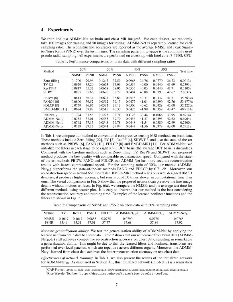
We train and test ADMM-Net on brain and chest MR images2. For each dataset, we randomlytake 100 images for training and 50 images for testing. ADMM-Net is separately learned for eachsampling ratio. The reconstruction accuracies are reported as the average NMSE and Peak Signal-to-Noise Ratio (PSNR) over the test images. The sampling pattern in k-space is the commonly usedpseudo radial sampling. All experiments are performed on a desktop with Intel core i7-4790k CPU.

Table 1: Performance comparisons on brain data with different sampling ratios.

Method 20% 30% 40% 50% Test timeNMSE PSNR NMSE PSNR NMSE PSNR NMSE PSNR

Zero-filling 0.1700 29.96 0.1247 32.59 0.0968 34.76 0.0770 36.73 0.0013sTV [2] 0.0929 35.20 0.0673 37.99 0.0534 40.00 0.0440 41.69 0.7391sRecPF [4] 0.0917 35.32 0.0668 38.06 0.0533 40.03 0.0440 41.71 0.3105sSIDWT 0.0885 35.66 0.0620 38.72 0.0484 40.88 0.0393 42.67 7.8637s

PBDW [6] 0.0814 36.34 0.0627 38.64 0.0518 40.31 0.0437 41.81 35.3637sPANO [10] 0.0800 36.52 0.0592 39.13 0.0477 41.01 0.0390 42.76 53.4776sFDLCP [8] 0.0759 36.95 0.0592 39.13 0.0500 40.62 0.0428 42.00 52.2220sBM3D-MRI [11] 0.0674 37.98 0.0515 40.33 0.0426 41.99 0.0359 43.47 40.9114s

Init-Net13 0.1394 31.58 0.1225 32.71 0.1128 33.44 0.1066 33.95 0.6914sADMM-Net13 0.0752 37.01 0.0553 39.70 0.0456 41.37 0.0395 42.62 0.6964sADMM-Net14 0.0742 37.13 0.0548 39.78 0.0448 41.54 0.0380 42.99 0.7400sADMM-Net15 0.0739 37.17 0.0544 39.84 0.0447 41.56 0.0379 43.00 0.7911s

In Tab. 1, we compare our method to conventional compressive sensing MRI methods on brain data.These methods include Zero-filling [22], TV [2], RecPF [4], SIDWT 3, and also the state-of-the-artmethods such as PBDW [6], PANO [10], FDLCP [8] and BM3D-MRI [11]. For ADMM-Net, weinitialize the filters in each stage to be eight 3 × 3 DCT basis (the average DCT basis is discarded).Compared with the baseline methods such as Zero-filling, TV, RecPF and SIDWT, our proposedmethod produces the best quality with comparable reconstruction speed. Compared with the state-of-the-art methods PBDW, PANO and FDLCP, our ADMM-Net has more accurate reconstructionresults with fastest computational speed. For the sampling ratio of 30%, our method (ADMM-Net15) outperforms the state-of-the-art methods PANO and FDLCP by 0.71 db. Moreover, ourreconstruction speed is around 66 times faster. BM3D-MRI method relies on a well designed BM3Ddenoiser, it produces higher accuracy, but runs around 50 times slower in computational time thanours. The visual comparisons in Fig. 5 show that the proposed network can preserve the fine imagedetails without obvious artifacts. In Fig. 6(a), we compare the NMSEs and the average test time fordifferent methods using scatter plot. It is easy to observe that our method is the best consideringthe reconstruction accuracy and running time. Examples of the learned nonlinear functions and thefilters are shown in Fig. 7.

Table 2: Comparisons of NMSE and PSNR on chest data with 20% sampling ratio.

Method TV RecPF PANO FDLCP ADMM-Net15-B ADMM-Net15 ADMM-Net17

NMSE 0.1019 0.1017 0.0858 0.0775 0.0790 0.0775 0.0768PSNR 35.49 35.51 37.01 37.77 37.68 37.84 37.92

Network generalization ability: We test the generalization ability of ADMM-Net by applying thelearned net from brain data to chest data. Table 2 shows that our net learned from brain data (ADMM-Net15-B) still achieves competitive reconstruction accuracy on chest data, resulting in remarkablea generalization ability. This might be due to that the learned filters and nonlinear transforms areperformed over local patches, which are repetitive across different organs. Moreover, the ADMM-Net17 learned from chest data achieves the better reconstruction accuracy on test chest data.

Effectiveness of network training: In Tab. 1, we also present the results of the initialized networkfor ADMM-Net13. As discussed in Section 3.1, this initialized network (Init-Net13) is a realization

2CAF Project: https://masi.vuse.vanderbilt.edu/workshop2013/index.php/Segmentation_Challenge_Details3Rice Wavelet Toolbox: http://dsp.rice.edu/software/rice-wavelet-toolbox

7

NMSE:0.0564; PSNR:35.79 NMSE:0.0727; PSNR:33.62 NMSE:0.0489; PSNR:37.03NMSE:0.0612; PSNR:35.10

NMSE:0.0660; PSNR:33.61 NMSE:0.0843; PSNR:31.51 NMSE:0.0726; PSNR:32.80 NMSE:0.0614; PSNR:34.22

Ground truth image

Ground truth image

Figure 5: Examples of reconstruction results with 20% (the first row) and 30% (the second row)sampling ratios. The left four columns show results of ADMM-Net15, RecPF, PANO, BM3D-MRI.

Test time in seconds(a) (b)

NM

SE

15

Stage number

Figure 6: (a) Scatter plot of NMSEs and average test time for different methods; (b) The NMSEs ofADMM-Net using different number of stages (20% sampling ratio for brain data).

Figure 7: Examples of learned filters in convolution layer and the corresponding nonlinear trans-forms (the first stage of ADMM-Net15 with 20% sampling ratio for brain data).

of the ADMM optimizing Eqn. (12). The network after training produces significantly improvedaccuracy, e.g., PNSR is increased from 32.71 db to 39.84 db with sampling ratio of 30%.

Effect of the number of stages: To test the effect of the number of stages (i.e., Ns), we greedily traindeeper network by adding one stage at each time. Fig. 6(b) shows the average testing NMSE valuesusing different stages in ADMM-Net under the sampling ratio of 20%. The reconstruction errordecreases fast when Ns < 8 and marginally decreases when further increasing the number of stages.

Effect of the filter sizes: We also train ADMM-Net initialized by two gradient filters with size of 1×3and 3 × 1 respectively for all convolution and reconstruction layers, the corresponding trained netwith 13 stages under 20% sampling ratio achieves NMSE value of 0.0899 and PSNR value of 36.52db on brain data, compared with 0.0752 and 37.01 db using eight 3 × 3 filters as shown in Tab. 1.We also learn ADMM-Net13 with 8 filters sized 5 × 5 initialized by DCT basis, the performance isnot significantly improved, but the training and testing time are significantly longer.

5 Conclusions

We proposed a novel deep network for compressive sensing MRI. It is a novel deep architecture de-fined over a data flow graph determined by an ADMM algorithm. Due to its flexibility in parameterlearning, this deep net achieved high reconstruction accuracy while keeping the computational effi-ciency of the ADMM algorithm. As a general framework, the idea that models an ADMM algorithmas a deep network can be potentially applied to other applications in the future work.

8

References[1] Michael Lustig, David L Donoho, Juan M Santos, and John M Pauly. Compressed sensing mri. IEEE

Journal of Signal Processing, 25(2):72–82, 2008.

[2] Michael Lustig, David Donoho, and John M Pauly. Sparse mri: The application of compressed sensingfor rapid mr imaging. Magnetic Resonance in Medicine, 58(6):1182–1195, 2007.

[3] Kai Tobias Block, Martin Uecker, and Jens Frahm. Undersampled radial mri with multiple coils: Iterativeimage reconstruction using a total variation constraint. Magnetic Resonance in Medicine, 57(6):1086–1098, 2007.

[4] Junfeng Yang, Yin Zhang, and Wotao Yin. A fast alternating direction method for tvl1-l2 signal recon-struction from partial fourier data. IEEE Journal of Selected Topics in Signal Processing, 4(2):288–297,2010.

[5] Chen Chen and Junzhou Huang. Compressive sensing mri with wavelet tree sparsity. In Advances inNeural Information Processing Systems, pages 1115–1123, 2012.

[6] Xiaobo Qu, Di Guo, Bende Ning, and et al. Undersampled mri reconstruction with patch-based directionalwavelets. Magnetic resonance imaging, 30(7):964–977, 2012.

[7] Saiprasad Ravishankar and Yoram Bresler. Mr image reconstruction from highly undersampled k-spacedata by dictionary learning. IEEE Transactions on Medical Imaging, 30(5):1028–1041, 2011.

[8] Zhifang Zhan, Jian-Feng Cai, Di Guo, Yunsong Liu, Zhong Chen, and Xiaobo Qu. Fast multi-classdictionaries learning with geometrical directions in mri reconstruction. IEEE Transactions on BiomedicalEngineering, 2016.

[9] Sheng Fang, Kui Ying, Li Zhao, and Jianping Cheng. Coherence regularization for sense reconstructionwith a nonlocal operator (cornol). Magnetic Resonance in Medicine, 64(5):1413–1425, 2010.

[10] Xiaobo Qu, Yingkun Hou, Fan Lam, Di Guo, Jianhui Zhong, and Zhong Chen. Magnetic resonance imagereconstruction from undersampled measurements using a patch-based nonlocal operator. Medical ImageAnalysis, 18(6):843–856, 2014.

[11] Ender M Eksioglu. Decoupled algorithm for mri reconstruction using nonlocal block matching model:Bm3d-mri. Journal of Mathematical Imaging and Vision, pages 1–11, 2016.

[12] Stephen Boyd, Neal Parikh, Eric Chu, Borja Peleato, and Jonathan Eckstein. Distributed optimization andstatistical learning via the alternating direction method of multipliers. Foundation and Trends in MachineLearning, 3(1):1–122, 2011.

[13] Huahua Wang, Arindam Banerjee, and Zhi-Quan Luo. Parallel direction method of multipliers. In Ad-vances in Neural Information Processing Systems, pages 181–189, 2014.

[14] Krishna M Kavi, Bill P Buckles, and U Narayan Bhat. A formal definition of data flow graph models.IEEE Transactions on Computers, 100(11):940–948, 1986.

[15] Yann Lécun, Leon Bottou, Yoshua Bengio, and Patrick Haffner. Gradient-based learning applied to docu-ment recognition. Proceedings of the IEEE, 86(11):2278–2324, 1998.

[16] Karol Gregor and Yann LeCun. Learning fast approximations of sparse coding. In Proceedings of the27th International Conference on Machine Learning, pages 399–406, 2010.

[17] Uwe Schmidt and Stefan Roth. Shrinkage fields for effective image restoration. In Proceedings of theIEEE Conference on Computer Vision and Pattern Recognition, pages 2774–2781, 2014.

[18] Sun Jian and Xu Zongben. Color image denoising via discriminatively learned iterative shrinkage. IEEETransactions on Image Processing, 24(11):4148–4159, 2015.

[19] John R Hershey, Jonathan Le Roux, and Felix Weninger. Deep unfolding: Model-based inspiration ofnovel deep architectures. arXiv preprint arXiv:1409.2574, 2014.

[20] Francis Bach, Rodolphe Jenatton, Julien Mairal, and Guillaume Obozinski. Optimization with sparsity-inducing penalties. Foundations and Trends in Machine Learning, 4(1):1–106, 2012.

[21] David E Rumelhart, Geoffrey E Hinton, and Ronald J Williams. Learning representations by back-propagating errors. Cognitive modeling, 5(3):1, 1988.

[22] Matt A Bernstein, Sean B Fain, and Stephen J Riederer. Effect of windowing and zero-filled reconstructionof mri data on spatial resolution and acquisition strategy. Magnetic Resonance Imaging, 14(3):270–280,2001.

9