decrease in stomach contents in the antarctic minke whale

SC/F14/J14

THIS PAPER CAN NOT BE CITED EXCEPT IN THE CONTEXT OF IWC MEETING UNTIL THE

PAPER IS FORMALLY PUBLISHED IN POLAR BIOLOGY

1

Kenji Konishi1•Takashi Hakamada

1• Hiroshi Kiwada

2•Toshihide Kitakado

3•Lars 2

Walløe4 3

Decrease in stomach contents in the Antarctic minke whale 4

(Balaenoptera bonaerensis) in the Southern Ocean 5

6

1Institute of Cetacean Research, 4-5, Toyomi-cho, Chuo-ku, Tokyo 104-0055, Japan 7

2Ocean Engineering & Development Co.,Ltd., 3-2 Nihonbashi Kobuna-cho, Chuo-ku, Tokyo 8

103-0024, Japan 9

3Tokyo University of Marine Science and Technology, 4-5-7, Kounan, Minato-ku, Tokyo 104-8477, 10

Japan 11

4 Department of Physiology, Institute of Basic Medical Sciences, University of Oslo, P.O. Box 1103 12

Blindern, N-0317 Oslo, Norway 13

14

E-mail: [email protected] 15

Tel: +81-3-3536-6521 16

Fax: +81-3-3536-6522 17

18

2

Abstract 19

The Antarctic minke whale (Balaenoptera bonaerensis) is one of the major krill predators in 20

Antarctic waters. A reported decline in energy storage over almost two decades indicates that food 21

availability for the whales may also have declined recently. To test this hypothesis, catch data from 22

20 survey years in the Japanese Whale Research Program in the Antarctic (JARPA) and its second 23

phase (JARPA II) (1990/91-2009/10), which covered the longitudinal sector between 35°E and 24

145°W south of 58°S, were used to investigate whether there was any annual trend in the stomach 25

contents of Antarctic minke whales. A linear mixed-effects analysis showed a 31% (95% CI 26

12.6%-45.3%) decrease in the weight of stomach contents over the 20 years since 1990/1991. A 27

similar pattern of decrease was found in both males and females, except in the case of females 28

sampled at higher latitude in the Ross Sea. These results suggest a decrease in the availability of krill 29

for Antarctic minke whales in the lower latitudinal range of the research area. The results are 30

consistent with the decline in energy storage reported previously. The decrease in krill availability 31

could be due to environmental changes or to an increase in the abundance of other krill-feeding 32

predators. The latter appears somewhat more likely, given the recent rapid recovery of humpback 33

whale. Furthermore, humpback whales are not found in the Ross Sea, where both Antarctic krill and 34

ice krill (E. crystallorophias) are available, and where no change in prey availability for Antarctic 35

minke whales is indicated. 36

37

KEYWORDS: Minke whale. Feeding ecology. Balaenoptera. Ross Sea. Antarctic krill 38

39

40

41

42

3

Introduction 43

The Antarctic minke whale (Balaenoptera bonaerensis) is a relatively small baleen whale species, but 44

a major component of the Southern Ocean ecosystem with an estimated abundance of over 500,000 45

the period 1992/93- 2003/04 (IWC 2012). The minke whale was not hunted until very near the end of 46

the commercial whaling period because of its small size, while other baleen whales, such as the blue 47

(Balaenoptera musculus), fin (B. physalus) and humpback whales (Megaptera novaeangliae), were 48

heavily depleted in the nineteenth and twentieth centuries. Laws (1977) therefore hypothesized that 49

the high population of minke whales in the 1980s was a response to the krill surplus resulting from the 50

reduction of the large baleen whales by commercial whaling. This hypothesis is based on the concept 51

of species interactions between krill predators, and has since been evaluated by modeling based on 52

population dynamics (Mori and Butterworth 2006). Nevertheless considerable controversy remains 53

about whether or not the large-scale removal of whales caused changes in the species composition of 54

other krill consumers, with some authors supporting “bottom-up” (Ballance et al. 2006; Nicol et al. 55

2007; Trivelpiece et al. 2011) and others “top-down” control theories (see Laws 1977; Reid and 56

Croxall 2001; Ainley et al. 2007)). According to the former, krill population dynamics and krill 57

availability for predators are controlled by production at lower trophic levels and oceanographic 58

conditions. The latter involve control by predation. Long time series of ecological and biological data 59

for baleen whales are needed to answer questions about ecosystem change in the Southern Ocean. 60

Energy storage in minke whales has been declining over a period of almost two decades (Konishi et 61

al. 2008), and the age at sexual maturity, which declined from the 1950s to the late 1960s, then 62

remained constant or increased slightly up to the 1990s (Zenitani and Kato 2006). These findings 63

could be signs of negative pressures on the Antarctic minke whale after the earlier increase in 64

population. They indicate that food availability may have declined in recent decades. In order to test 65

this hypothesis, we used a 20-year time series of data on stomach contents obtained by the Japanese 66

Whale Research Program under Special Permit in the Antarctic (JARPA) and its second phase 67

(JARPA II). 68

69

Materials and Methods 70

Research area and period 71

4

JARPA was conducted during the austral summer seasons (December to March) from 1987/1988 to 72

2004/2005, while JARPA II started in the 2005/2006 season and is still continuing. Data used in the 73

present study were collected between the 1990/91 and 2009/10 seasons. These long-term programs 74

include whale sampling to study biological parameters concurrently with sighting surveys and 75

oceanographic surveys for management and monitoring purposes (Government of Japan 2005). The 76

research area for the research programs is the longitudinal sector between 35°E and 145°W, south of 77

60°S (and a few catches between 58°S and 60°S in JARPA). This sector includes the Management 78

Areas IIIE, IV, V and VIW of the International Whaling Commission (Donovan 1991; Fig. 1). The 79

Ross Sea is the highest-latitude part of the study area, between 170°E and 160°W and south of 70°S. 80

It lies largely above the continental shelf and is shallower than 1000m. 81

Samples 82

Antarctic minke whales were randomly sampled along predetermined tracklines. Sampling was 83

carried out from one hour after sunrise to one hour before sunset, but limited to a maximum of 12 84

hours per day. The sampling positions for the Antarctic minke whales used in this study are shown in 85

Figure 1. The number of samples used in the present study is shown in Table 1 for each sex. Samples 86

were taken in the Ross Sea every second year, and Table 2 indicates the years when samples were 87

taken in lower and higher latitudinal areas. The search lines and the positions where whales were 88

found indicate where krill was available (Online Resource 1). 89

Examination of stomach contents 90

All whales were dissected on board the research base vessel Nisshin-Maru. Stomach contents were 91

removed from each compartment and weighed to the nearest 0.1kg, and some subsamples were 92

collected for species identification. Details of the treatments of stomach contents were given in 93

Tamura and Konishi (2009). Minke whales have a four-chambered stomach (Hosokawa and Kamiya 94

1971; Olsen et al. 1994), and the forestomach serves mainly as a food storage chamber, like the rumen 95

in bovids (Olsen et al. 1994). For statistical analysis, we used the weight of the sieved contents of the 96

forestomach as the weight of the stomach contents (kg: SCW) which is the most consistent measure 97

throughout JARPA - JARPA II period, with the exception of the first three seasons (1987/88 - 98

1989/90), when forestomach contents were not weighed. Since whales were caught during the day, 99

5

the diurnal feeding pattern had to be included in the models. The weight of stomach contents showed 100

a decline from morning to evening in a previous study (Tamura and Konishi 2009). 101

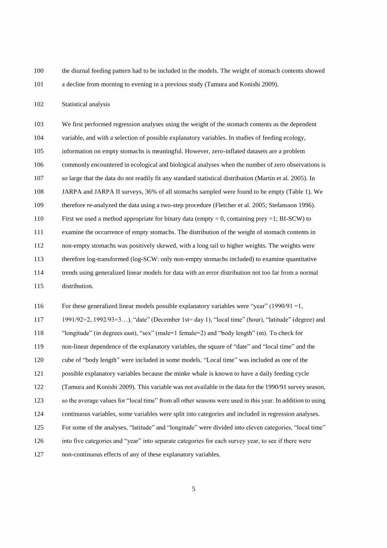
Statistical analysis 102

We first performed regression analyses using the weight of the stomach contents as the dependent 103

variable, and with a selection of possible explanatory variables. In studies of feeding ecology, 104

information on empty stomachs is meaningful. However, zero-inflated datasets are a problem 105

commonly encountered in ecological and biological analyses when the number of zero observations is 106

so large that the data do not readily fit any standard statistical distribution (Martin et al. 2005). In 107

JARPA and JARPA II surveys, 36% of all stomachs sampled were found to be empty (Table 1). We 108

therefore re-analyzed the data using a two-step procedure (Fletcher et al. 2005; Stefansson 1996). 109

First we used a method appropriate for binary data (empty = 0, containing prey =1; BI-SCW) to 110

examine the occurrence of empty stomachs. The distribution of the weight of stomach contents in 111

non-empty stomachs was positively skewed, with a long tail to higher weights. The weights were 112

therefore log-transformed (log-SCW: only non-empty stomachs included) to examine quantitative 113

trends using generalized linear models for data with an error distribution not too far from a normal 114

distribution. 115

For these generalized linear models possible explanatory variables were “year” (1990/91 =1, 116

1991/92=2, 1992/93=3…), “date” (December 1st= day 1), “local time” (hour), “latitude” (degree) and 117

“longitude” (in degrees east), “sex” (male=1 female=2) and “body length” (m). To check for 118

non-linear dependence of the explanatory variables, the square of “date” and “local time” and the 119

cube of “body length” were included in some models. “Local time” was included as one of the 120

possible explanatory variables because the minke whale is known to have a daily feeding cycle 121

(Tamura and Konishi 2009). This variable was not available in the data for the 1990/91 survey season, 122

so the average values for “local time” from all other seasons were used in this year. In addition to using 123

continuous variables, some variables were split into categories and included in regression analyses. 124

For some of the analyses, “latitude” and “longitude” were divided into eleven categories, “local time” 125

into five categories and “year” into separate categories for each survey year, to see if there were 126

non-continuous effects of any of these explanatory variables. 127

6

An important assumption in fixed effects models is that data are independent. Since JARPA and 128

JARPA II sampling surveys were conducted in each survey seasons in only a part of the total sampling 129

area, this assumption may be violated, and the data matrix may contain spatio-temporal correlations 130

because the environmental factors driving the results are correlated. The use of random effect models 131

is one common and convenient way to model such data structure (Faraway 2006), and we therefore 132

included some random effects by some of the categorical variables in our models. 133

For first analyses with BI-SCW as the dependent variable, we used a linear mixed-effects logistic 134

model with a logit link function. In the main analyses with log-SCW as the dependent variable, we 135

used a linear mixed effects model, and the estimation was effected using restricted maximum 136

likelihood methods (REML) (Baayen et al. 2008). The continuous variable “year” was included in all 137

models to examine the linear yearly trend in stomach contents. To compare models and determine the 138

most plausible model, the Akaike’s Information Criterion (AIC) was used and the three models with 139

smallest AIC were chosen as plausible models. We ran the various regression models including and 140

excluding explanatory variables from the simple basic model (LMER1; Online Resource 2) and used 141

AIC to show differences from the basic model. Since inferences regarding the fixed-effect parameters 142

are more complicated in a linear mixed-effects model (Baayen et al. 2008), we also applied the Markov 143

chain Monte Carlo (MCMC) technique with 10000 resamplings to estimate confidence intervals and 144

p-value for year effects for each model. The main analyses were conducted for both sexes combined 145

and the best models were selected. To investigate possible correlation between years, the jack-knife 146

method was applied in one of the best models by excluding data from one year at a time. To confirm 147

the jack-knife results, track line as a grouping factor for random effects was added into one of the 148

best models. The analyses were also carried out without data from the first year (when ‘local time’ 149

was not available). None of these analyses changed the conclusions. Analyses were then performed 150

for males and females separately without the “sex” variable, using the three best models identified 151

from the analyses for both sexes combined. Because the distribution of females covered such a wide 152

range of latitudes, extending as far south as the Ross Sea (Figure 1), data from females were analyzed 153

separately for lower and higher latitude areas, with 70°S as the dividing line. For these analyses, 154

“latitude” was divided into twenty categories. Because there were few males in the higher latitude area 155

(Table 2), data from lower latitudes for both sexes were analyzed to see the results without any effect 156

of higher latitude. To confirm the robustness of the year effect in the analyses with respect to the 157

7

statistical assumptions, the best models in Log-SCW were also run using ranked SCW and the original 158

nontransformed SCW datasets. 159

All statistical analyses were conducted in R environment version 2.13 (R development core team 160

2011) using package “lme4” version 0.999375-41 (Faraway 2006; Bates 2007), “languageR” version 161

1.2 (Baayen 2011) for mixed effects models and “LMERConvenientFunctions” (Tremblay 2011) for 162

graph illustration. 163

164

Results 165

In the first step, a total of eleven mixed effect logistic regressions using BI-SCW data (Table 3) were 166

used to analyze whether there was any time trend from year to year in the proportion of empty 167

stomachs for the two sexes combined. No statistically significant estimates of the coefficient for “year” 168

(year effect) were found in any of the regression analyses. The regression coefficients ranged from 169

-0.0061 to 0.0009 per year. These results show that there was no trend in the proportion of empty 170

stomachs in Antarctic minke whales through the survey period. The effect of “local time” was 171

statistically significant in all runs with an increase in empty stomachs of about 2% per hour from dawn 172

to dusk. 173

Since no trend in the proportion of empty stomachs was evident, log transformed data from non-empty 174

stomachs (log-SCW) were used for next analyses. For the main analyses for the two sexes combined, 175

we used 24 mixed effects models including the explanatory variables (see Online Resource 2). In all 176

regression models, the year effects were similar and ranged from -0.026 to -0.018 per year. They were 177

significant at the 5% level in all models (Online Resource 3). The year effects indicate that the 178

stomach contents of Antarctic minke whales have decreased substantially with time. The model 179

LMER24, including crossed random effects of “date2” grouped by categorical variables “year” and 180

“latitude”, and “date2” grouped by categorical variables “longitude” and “year”, gave the smallest AIC, 181

followed by models LMER16 and LMER23. The coefficients of “local time”, “sex” and “body length” 182

in LMER24 were -0.115 per hour, -0.128 less for females than males, and 0.311 per meter, 183

respectively, indicating that minke whales with food in their stomach have fed more early in the day, 184

and that males and larger individuals feed more (Table 4). The scatterplot of standardized residuals in 185

8

LMER24 shows that the distribution is acceptable for a parametric approach (Figure 2). Although it 186

is still somewhat skewed even after the log transformation, the distribution is not too far from normal. 187

To explore possible biases, we have run some additional checks. In the jack-knife analysis, the mean 188

effect of ‘year’ for 20 runs was -0.020 (95% C I: -0.027 to -0.012), showing that the effect of ‘year’ 189

is stable between years, which suggests that there was little correlation between years. Random 190

effects of ’date’, ’latitude’ and ’longitude’ grouped by track line were added into LMER24, giving 191

similar negative ‘year’ effects at the 5% significant level (random effects of ‘date’ -0.020, SE: 192

0.0062, ‘latitude’ -0.026, SE: 0.0073, ‘longitude’ -0.031, SE: 0.0070). When the best three models 193

were fitted to the data set for lower latitudes only, the results were similar to those for the whole area 194

(Online Resource 3). The LMER 24 was also fitted to the data set without data from the first year as 195

a sensitivity test for missing ‘local time’ in the first year, giving results similar to those from all 196

years (coefficient of -0.0246, p< 0.001). This model was also fitted to the total data set, including 197

both empty stomachs and stomachs with contents. The results were a ‘year’ effect of -0.338 (SE: 198

0.057, p<0.0001). These additional analyses all support the results of the mixed-effects models. 199

As the next step, the three best models (LMER16, 23 and 24) identified in the earlier set of analyses 200

were applied separately to the male-only and female-only dataset (Online Resource 3). The year 201

effects in males were similar in the three models, ranging from -0.0278 to -0.0270 per year, and were 202

significant at the 5% level. This is of the same order as in the analyses for the two sexes combined, 203

showing a clear decrease of stomach contents over time in males. However, the ‘year’ effects in 204

females were not significant in the three models (Online Resource 3). Because the distribution of 205

females covers a wider range of latitudes, an area effect (lower and higher latitude areas, north and 206

south of 70°S) against ‘year’ was included in the three best models for the female-only dataset. In 207

two of the models, the area effects were significant at the 5% level (Online Resource 3), showing 208

that the ‘year’ effects differ between the two latitude areas. Then the analyses were performed for 209

two datasets separately, that is for females at lower and higher latitudes (Online Resource 3). In the 210

analyses for females at lower latitudes, the year effects ranged from -0.0236 to -0.0215, which is 211

significant at the 5% level. In the analyses for females at higher latitudes (including the Ross Sea), the 212

coefficients of “year” show a small positive slope with large p-values, which means that no time trend 213

in stomach contents was found for females in this area (Online Resource 3). 214

9

Additional regression analyses using ranked SCW and the original (nontransformed) SCW were 215

conducted as robustness trials. The results are shown in Table 5. All year effects are negative with a 216

significance probability of less than 5% except in one case. These results add support to the main 217

regression results, which use log-SCW as the dependent variable. 218

219

Discussion 220

All the main regression analyses for both sexes show that the year effects on the weight of stomach 221

contents are negative, indicating that food intake by Antarctic minke whales has decreased over the 222

20-year period. Based on the best model, the rate of decrease in stomach contents is exp(-0.0194) or 223

1.96% pa and the average SCW of non-empty stomachs is 25.62 kg. We used this as the average value 224

for SCW in the 10th year (1999/2000). SCW in the first and last years can then be calculated as 225

25.62*exp(-0.0194)^(-9) and 25.62*exp(0.0194)^(10). In this way, the decrease in stomach content 226

weight through the whole survey period was found to be approximately 9.41 kg (95%CI 3.44-15.42), 227

or 31% (95%CI 12.6-45.3) of the mean weight in the first year (which is estimated at 30.5 kg). This 228

large decrease is consistent with the results of earlier studies on energy storage (Konishi et al. 2008) 229

and age at maturity (Zenitani and Kato 2006). A possible explanation for the results of all three 230

investigations is that prey availability for minke whales has decreased in recent decades. As a 231

supplement to the analyses in Konishi et al. (2008), blubber thicknesses from their study were 232

reanalyzed using a linear mixed-effects model to examine year effects as in the present investigation. 233

The results showed a negative year trend similar to the values obtained by Konishi et al. (2008) (Skaug 234

2011). 235

In the logistic regression analyses using binary SCW, no time trend in the proportion of empty 236

stomachs was observed. This indicates that the weight of the stomach contents is independent of the 237

reason for empty forestomachs in minke whales. The occurrence of empty stomachs is probably 238

related to the feeding behavior of minke whales. The Antarctic minke whale has a daily feeding 239

cycle, feeding most actively in the morning, but with individual variation between whales (see 240

Tamura and Konishi 2009), and this could explain the absence of food in the forestomachs at certain 241

times of day. Furthermore, aggregation of Antarctic krill is not uniform in the study area (see Sara et 242

10

al. 2002; Taki et al. 2008), and minke whales may therefore not feed while moving between krill 243

aggregations. The time series appears to be consistent with this feeding pattern. 244

A reviewer has suggested that a harpooned whale might vomit part of its stomach contents if the kill 245

is not instantaneous, and that this might bias the results of our analyses. Vomiting has never been 246

observed in harpooned minke whales, even when there have been systematic observations since the 247

first year of JARPA II to attempt to detect this. Nevertheless, to examine this possibility further, 248

information on whether the kill was instantaneous or not (using the death criteria as agreed by the 249

IWC) was added as a new binomial variable, and the best fitted model LMER 24 was run both with 250

and without this variable. This information was not available for the first six years of JAPRA, so the 251

two models were run for the last 15 years of JARPA and JARPA II only. During these years about 252

40% of the whales were killed instantaneously. Both models gave virtually the same rate of decline 253

in stomach contents with year, which for both models was statistically highly significant. AIC 254

increased when the instantaneous death variable was added to the models, and the coefficient for this 255

new variable was very small and far from significant. These results are not consistent with the 256

possibility of vomiting leading to a bias in our estimate of the rate of decline in stomach contents. 257

Year effects were negative in males and in females at lower latitudes, while no year effect was 258

observed in females at higher latitudes, including the Ross Sea. This indicates that prey availability 259

has decreased north of 70 °S, but not in the Ross Sea. This can be explained by the fact that different 260

krill species are available in the southern Ross Sea and other areas, and by the overlap in distribution 261

between minke whales and humpback whales. Minke whales have a sex-segregated distribution 262

pattern, and pregnant females occur at high density in the Ross Sea (Kato et al. 1991; Ichii et al. 1998), 263

especially above the continental shelf in areas shallower than 1000 m. In this area, ice krill E. 264

crystallorophias is common and is the most important prey of the Antarctic minke whales (see Ichii et 265

al. 1998; Tamura and Konishi 2009), while the Antarctic krill (Sala et al. 2002; Taki et al. 2008) is 266

only occasionally found in this area. Ice krill probably functions as a stable prey species for minke 267

whales, and its abundance shows no correlation with that of the Antarctic krill, which suggests that 268

evidence of a decrease in krill availability would not be expected in this area. In contrast, the results 269

here suggest that a decline in krill availability for minke whales has occurred in the main distribution 270

area of Antarctic krill, north of the continental shelf. Humpback whales occur in the offshore area, 271

with almost no observations south of 70°S in the study area (see Matsuoka et al. 2005; Matsuoka et 272

11

al. in press), suggesting that interactions with the Antarctic minke whale are only likely north of 273

70°S. Fin whales also occur in the study area, but tend only to be present in small numbers in 274

offshore waters (see Matsuoka et al. 2005). These possible interactions are described in more detail 275

below. 276

A 31% reduction in food intake as measured by stomach content weight of the Antarctic minke whale 277

over two decades needs to be taken into account in quantitative studies of the Antarctic ecosystem 278

such as the modeling studies by Mori and Butterworth (2006) because the species is such an 279

important consumer. Total consumption by minke whales in the feeding season was estimated at 280

approximately 1.1 million tonnes in 2001/02 in IWC management area IV and 4.1 million tonnes in 281

2002/03 in area V, corresponding to the western part of this study area (Tamura and Konishi 2009), 282

and annual consumption by mature animals was estimated at 35.5 million tonnes south of 60°S in the 283

1970s and 1980s (Armstrong and Siegfried 1991). 284

Possible changes in the abundance of minke whales, krill and other krill predators are important in 285

any discussion of the reasons for the decrease in stomach contents in minke whales (Plagányi and 286

Butterworth 2012). Intra-species interactions can reduce food availability per capita if minke whale 287

abundance in the feeding areas is close to carrying capacity. However, the abundance of Antarctic 288

minke whales in ice-free areas most likely decreased from the 1970s to the early 2000s (Branch and 289

Butterworth 2001; IWC 2012) and age at sexual maturity stopped declining in the 1970s (Zenitani 290

and Kato 2006), so that it is unlikely that the decline in krill availability was caused by intra-species 291

interactions such as an increase in minke whale abundance in the study area. Two alternative 292

hypotheses can be suggested to explain the decline in krill availability for minke whales, especially 293

at the lower latitudes of the study area. The first is that krill availability for the Antarctic minke 294

whales has changed in response to oceanographic and environmental changes. The oceanographic 295

environment is an important factor for krill abundance and distribution (Sala et al. 2002). The most 296

obvious changes around the Antarctic Peninsula are due to global warming (Meredith 2005): rising 297

temperature and increasing current strength is resulting in a decrease in sea ice extent and duration, 298

which causes low blooming success and a low density of krill (Loeb et al. 1997; Atkinson et al. 2004; 299

Siegel 2005; Siegel and Loeb 1995; Trathan et al. 2003; Hunt and Hosie 2006; Nicol 2006). Scientific 300

echo sounders were carried on board to collect data on krill abundance during JARPAII 301

(Government of Japan 2005), but no results on trends in krill abundance are available from the study 302

12

area at present. Changes in temperature, sea ice thickness and the extent and persistence of polynyas 303

have been observed in the study area (see Ainley et al. 2010; Comiso et al. 2011), and these 304

environmental changes could be affecting krill reproduction in the study area. Further information is 305

needed to make projections of krill population trends. 306

A second hypothesis to explain the decrease in krill availability is interactions between krill predators. 307

West of the Antarctic Peninsula, the recovery of baleen whale and fur seal populations is one of the 308

reasons suggested for the decline in krill availability to penguins (Trivelpiece et al. 2011). Different 309

studies indicate that the recovery of the populations of humpback, fin and blue whales started more 310

than twenty years ago (Bannister 1994; Matsuoka et al. 2005; Branch 2006; Branch; 2007; Noad et al. 311

2011). In particular, the annual rate of increase in humpback whale abundance in Area IV has been 312

over 12% during the JARPA survey period (1989/1990-2004/2005), and abundance was estimated at 313

approximately 37000 whales in this area after 2000 (Matsuoka et al. in press). This is higher than the 314

estimated minke whale biomass in Area IV (see Matsuoka et al. 2005; Matsuoka et al. in press). In the 315

study area, the humpback whale feeds on the Antarctic krill (Mizue and Murata 1951; Kawamura 316

1978; Stone and Hamner 1988). The two whale species may have different spatial feeding patterns to 317

avoid “direct” competition or maintain spatial niche separation (see Kasamatsu et al. 2000; 318

Friedlaender et al. 2009; Santora et al. 2010). However, minke and humpback whale distributions 319

overlap between 60 and 65°S (see Murase et al. 2002), suggesting that they share the same krill 320

resources. Furthermore, humpback whale biomass was less than half of minke whale biomass in the 321

early 1990s, but rose to more than twice total minke whale biomass by the early 2000s in Area IV 322

(see Matsuoka et al. 2005). Thus, the rapid recovery of the humpback whale is likely to have reduced 323

krill availability for the minke whale, although a decline in the krill population in response to 324

environmental change may have accelerated the decline and thus its availability for the minke whale. 325

We have demonstrated consistent long-term changes in the nutritional status of the Antarctic minke 326

whale in the JARPA research area. However, we need to be cautious in interpreting the scale and 327

other details of the decline, because whales presumably change their feeding behavior in response to 328

changes in food availability. For instance, whales are expected to compensate for lower food density 329

by travelling further in search of food and more lunge feeding, but the latter has high energetic costs, 330

especially in large whales (Acevedo-Gutiérrez et al. 2002; Goldbogen et al. 2006; Goldbogen et al. 331

2008). For a deeper understanding of minke whale feeding, we need to know whether and how minke 332

13

whales have changed their distribution to adapt to the change in food availability. According to an 333

ecosystem model developed on the assumption that krill predators compete, species other than baleen 334

whales, such as crabeater seals (Lobodon carcinophagus), may play an important role (Mori and 335

Butterworth 2006). Thus there is also a need to investigate how the other important krill predators 336

interact with each other and with minke whales in order to gain a deeper understanding of the Antarctic 337

minke whale’s environment. If future studies provide this information, it may help to confirm or reject 338

the krill surplus hypothesis put forward by Laws (1977). If the decrease in food availability for minke 339

whales continues, the population will decline, partly as a result of the rise in age at sexual maturity. 340

Thus, continuous monitoring of food availability as indicated by stomach contents and of energy 341

storage in the form of blubber thickness can contribute important information for the management 342

and conservation under the mandates of both the IWC and CCAMLR of the krill fishery and of the 343

predators that depend on krill for food in the Southern Ocean. Such monitoring may also give 344

information about the extent to which changes in abundance of krill are driven by top-down 345

(consumption) compared to bottom-up (environmental) effects. 346

347

ACKNOWLEDGEMENTS 348

We would like to thank all the captains, crews, especially Hajime Shirasaki (Kyodo Senpaku Co. Ltd.) 349

and the scientists who were involved in the JARPA and JARPAII surveys. Thanks are also due to T. 350

Tamura, S. Kumagai, L.A. Pastene, H. Skaug and D. Butterworth for their useful comments on the 351

manuscript, and to Alison Coulthard for correcting the English. The JARPA program was conducted 352

with permission from the Japanese Fisheries Agency, Government of Japan. 353

354

14

REFERENCES 355

Acevedo-Gutiérrez A, Croll DA, Tershy BR (2002) High feeding costs limit dive time in the largest 356

whales. J Exper Biol 205: 1747-1753. 357

Ainley D, Ballard G, Ackley S, Blight LK, Eastman JT, Emslie SD, Lescroël A, Olmastroni S, 358

Townsend SE, Tynan CT, Wilson P, Woehler E (2007) Paradigm lost, or is top-down forcing no 359

longer significant in the Antarctic marine ecosystem? Ant Sci 19:283-290. 360

doi:10.1017/S095410200700051X 361

Ainley D, Russell J, Jenouvrier S, Woehler E, Lyver P, Fraser WR, Kooyman GL (2010) Antarctic 362

penguin response to habitat change as Earth’s troposphere reaches 28C above preindustrial levels. 363

Ecol Monogr 801: 49–66. doi:10.1890/08-2289.1 364

Armstrong AJ, Siegfried WR (1991) Consumption of Antarctic krill by Minke whales. Ant Sci 365

3:13-18. doi:10.1017/S0954102091000044 366

Atkinson A, Siegel V, Pakhomov E, Rothery P. (2004) Long-term decline in krill stock and increase in 367

salps within the Southern Ocean. Nature 432;100-103. doi:10.1038/nature02996 368

Baayen R H (2011) languageR: Data sets and functions with "Analyzing Linguistic Data: A practical 369

introduction to statistics". R package version 1.2. http://CRAN.R-project.org/package=language 370

Baayen RH, Davidson DJ, Bates DM (2008) Mixed-effects modeling with crossed random effects for 371

subjects and items. J Mem Lang 59:390-412. doi:10.1016/j.jml.2007.12.005 372

Ballance LT, Pitman RL, Hewitt RP, Siniff DB, Trivelpiece WZ, Clapham PJ, Brownell LB (2006) In: 373

Estes A et al. (eds) Whales, whaling and ocean ecosystems. University of California Press, pp 215–374

230 375

Bannister J L (1994) Continued increase in humpback whales off western Australia. Rep Int Whal 376

Commn 44: 309- 310. 377

Bates DM (2007) Linear mixed model implementation in lme4. Manuscript, university of Wisconsin - 378

Madison, January 2007. 379

15

Beekmans BWPM, Forcada J, Murphy E, de Baar HJW, Bathmann UV, Fleming AH (2010). 380

Generalised additive models to investigate environmental drivers of Antarctic minke whale 381

(Balaenoptera bonaerensis) spatial density in austral summer. J Cetacean Res Manage 11:115–129. 382

Branch TA (2006) Humpback abundance south of 60°S from three completed sets of IDCR/SOWER 383

circumpolar surveys. IWC Document SC/AO6/HW6: 14pp 384

Branch, TA (2007) Abundance of Antarctic blue whales south of 60 S from three complete 385

circumpolar sets of surveys. J Cetacean Res Manage. 9:253–262. 386

Branch TA, Butterworth DS (2001). Southern Hemisphere minke whales: standardised abundance 387

estimates from the 1978/79 to 1997/98 IDCR-SOWER surveys. J Cetacean Res Manage 3:143-174. 388

Comiso JC, Kwok R, Martin S, Gordon AL (2011) Variability and trends in sea ice extent and ice 389

production in the Ross Sea. J Geophys Res 116: 1-19. doi:10.1029/2010JC006391. 390

Donovan GP (1991) A review of IWC stock boundaries (special issue). Rep int Whal Commn 13: 391

39-68 392

Faraway JJ (2006) Extending the linear model with R. Boca Raton, FL: Chapman & Hall/CRC. pp 393

331. 394

Friedlaender AS, Lawson GL, Halpin PN (2009) Evidence of resource partitioning between humpback 395

and minke whales around the western Antarctic Peninsula. Mar Mamm Sci 25:402-415. 396

doi:10.1111/j.1748-7692.2008.00263.x 397

Fletcher D, MacKenzie D, Villouta E (2005). Modelling skewed data with many zeros: A simple 398

approach combining ordinary and logistic regression. Environ Ecol Stat 12:45–54. 399

doi:10.1007/s10651-005-6817-1 400

Goldbogen JA, Calambokidis J, Shadwick RE, Oleson EM, McDonald MA, Hildebrand JA (2006) 401

Kinematics of foraging dives and lunge-feeding in fin whales. J Exper Biol 209: 1231-1244. 402

doi:10.1242/jeb.02135 403

16

Goldbogen JA, Calambokidis J, Croll, DA, Harvey JT, Newton KM, Oleson EM, Schorr G, Shadwick 404

RE (2008) Foraging behavior of humpback whales: kinematic and respiratory patterns suggest a high 405

cost for a lunge. J Exper Biol 211: 3712-3719. doi:10.1242/jeb.023366 406

Government of Japan (2005) Plan for the Second Phase of the Japanese Whale Research Program 407

under Special Permit in the Antarctic (JARPA II) -Monitoring of the Antarctic Ecosystem and 408

Development of New Management Objectives for Whale Resources. Paper SC/57/O1 presented to the 409

IWC Scientific Committee, Jun 2005. 99pp. 410

Hunt B, Hosie G (2006) The seasonal succession of zooplankton in the Southern Ocean south of 411

Australia, part I: The seasonal ice zone. Deep Sea Res I 53:1182-1202. doi:10.1016/j.dsr.2006.05.001. 412

International Whaling Commission (2012) Report of the Sub-Committee on Abundance estimate on 413

the Antarctic minke whale. Rep Int Whal Comm (available on IWC web page) 35-39. 414

Ichii T, Shinohara N, Fujise Y, Nishiwaki S, Matsuoka K. (1998) Interannual changes in body fat 415

condition index of minke whales in the Antarctic. Mar Ecol Prog Ser 175:1-12. 416

doi:10.3354/meps175001 417

Kasamatsu F, Matsuoka K, Hakamada T (2000) Interspecific relationships in density among the whale 418

community in the Antarctic. Polar Biol 23:466-473. doi:10.1007/s003009900107 419

Kato H, Fujise Y, Kishino H (1991). Age structure and segregation of southern minke whales by the 420

data obtained during Japanese research take in 1988/89. Rep Int Whal Commn 41:287-292 421

Kawamura A (1978) An interim consideration on a possible interspecific relation in southern baleen 422

whales from the viewpoint of their food habits. Rep Int Whal Commn 28:411-420 423

Konishi K, Tamura T, Zenitani R, Bando T, Kato H, Walløe L (2008) Decline in energy storage in the 424

Antarctic minke whale (Balaenoptera bonaerensis) in the Southern Ocean. Polar Biol 31:1509-1520. 425

doi:10.1007/s00300-008-0491-3 426

Laws RM (1977) Seals and whales of the Southern Ocean. Phil Trans R Soc Lond B 279:81-96. 427

doi:10.1098/rstb.1977.0073 428

17

Loeb V, Siegel V, Holm-Hansen O, Hewitt R, Fraser W, Trivelpiece W, Trivelpiece S (1997) Effects 429

of sea-ice extent and krill or salp dominance on the Antarctic food web. Nature 387:897-900. 430

doi:10.1038/43174 431

Martin T, Wintle B, Rhodes J, Kuhnert P, Field S, Low-Choy S, Tyre A, Possingham, H (2005) Zero 432

tolerance ecology: improving ecological inference by modelling the source of zero observations. Ecol 433

lett 8:1235-1246. doi:10.1111/j.1461-0248.2005.00826.x 434

Matsuoka K, Hakamada T, Kiwada H, Murase H, Nishiwaki S (2005) Abundance increases of large 435

baleen whales in the Antarctic based on the sighting survey during Japanese Whale Research Program 436

(JARPA). Glob Environ Res 9:105-115 437

Matsuoka K, Hakamada T, Kiwada H, Murase H, Nishiwaki S (in press) Abundance estimates and 438

trends for humpback whales (Megaptera novaeangliae) in Antarctic Areas IV and V based on JARPA 439

sighting data. J Cetacean Res Manage Special Issue: Southern Hemisphere humpback whale 440

Meredith MP (2005) Rapid climate change in the ocean west of the Antarctic Peninsula during the 441

second half of the 20th century. Geophys Res Lett 32: 1-5. doi:10.1029/2005GL024042. 442

Mizue K, Murata T (1951) Biological Investigation on the whales caught by the Japanese Antarctic 443

whaling fleets season 1949-50. Sci Rep Whales Res Ins Tokyo 6:73-131 444

Mori M, Butterworth DS (2006) A first step towards modelling the krill-predator dynamics of the 445

Antarctic ecosystem. CCAMLR Sci 13:217–277 446

Murase H, Matsuoka K, Ichii T, Nishiwaki S (2002) Relationship between the distribution of 447

euphausiids and baleen whales in the Antarctic (35 E-145 W). Polar Biol 25: 135-145. 448

doi:10.1007/s003000100321. 449

Nicol S. (2006) Krill, currents, and sea ice: Euphausia superba and its changing environment. BioSci 450

56: 111-120. doi:10.1641/0006-3568(2006)056. 451

Nicol S, Croxall J, Trathan P, Gales N, Murphy E (2007) Paradigm misplaced? Antarctic marine 452

ecosystems are affected by climate change as well as biological processes and harvesting. Ant Sci 453

19:291. doi:10.1017/S0954102007000491 454

18

Noad MJ, Dunlop RA,Paton D, Kniest H (2011) Abundance estimates of the east Australian 455

humpback whale population: 2010 survey and update. Paper IWC/SC/63/SH22 (Available at IWC 456

web page: http://iwcoffice.org). 457

Olsen MA., Nordøy E S, Blix AS, Mathiesen SD (1994) Function anatomy of the gastrointestinal 458

system of Northeastern Atlantic minke whales (Balaenoptera acutorostrata). J Zool Lond 234: 55-74. 459

doi:10.1111/j.1469-7998.1994.tb06056.x 460

Plagányi EE and Butterworth DS (2012) The Scotia Sea krill fishery and its possible impacts on 461

dependent predators – modeling localized depletion of prey. Ecol Monogr 22:748–761. doi: 462

10.1890/11-0441.1 463

R Development Core Team (2011) R: A language and environment for statistical computing. R 464

Foundation for Statistical Computing, Vienna, Austria. ISBN 3-900051-07-0, URL 465

http://www.R-project.org. 466

Reid K, Croxall JP (2001) Environmental response of upper trophic-level predators reveals a system 467

change in an Antarctic marine ecosystem. Proc R. Soc Lond B 268:377-384. 468

doi:10.1098/rspb.2000.1371 469

Sala A, Azzali M, Russo A (2002) Krill of the Ross Sea: distribution, abundance and demography of 470

Euphausia superba and Euphausia crystallorophias during the Italian Antarctic Expedition 471

(January-February 2000). Sci Mar 66:123-133. doi:10.3989/scimar.2002.66n2123 472

Santora J, Reiss C, Loeb V, Veit R (2010) Spatial association between hotspots of baleen whales and 473

demographic patterns of Antarctic krill Euphausia superba suggests size-dependent predation. Mar 474

Ecol Prog Ser 405:255-269. doi:10.3354/meps08513 475

Siegel V, Loeb V (1995) Recruitment of Antarctic krill Euphausia superba and possible causes for its 476

variability. Mar Ecol Prog Ser 123: 45-56. doi:10.3354/meps123045. 477

Siegel V (2005) Distribution and population dynamics of Euphausia superba: summary of recent 478

findings. Polar Biol 29: 1-22. doi:10.1007/s00300-005-0058-5. 479

Skaug (2011) Results of mixed-effects regression analyses of blubber thickness in Antarctic minke 480

whale from data collected under JARPA. Appendix 2 in IWC/63/Rep 1 Report of the Scientific 481

19

Committee Annex K1: Working Group to Address Multi-species and Ecosystem Modelling 482

Approaches, Tromsø, Norway, 30 May to 11 June 2011. (Available at IWC web page: 483

http://iwcoffice.org). 484

Stefansson G (1996) Analysis of groundfish survey abundance data: combining the GLM and delta 485

approaches. ICES J Mar Sci 53:577–588 486

Stone GS, Hamner WM (1988) Humpback whales Megaptera novaeangliae and southern right whales 487

Eubalaena australis in Gerlache Strait, Antarctica. Polar Rec 24:15-20. 488

doi:10.1017/S0032247400022300 489

Taki K, Yabuki T, Noiri Y, Hayashi T, Naganobu M (2008) Horizontal and vertical distribution and 490

demography of euphausiids in the Ross Sea and its adjacent waters in 2004/2005. Polar Biol 491

31:1343-1356. doi: 10.1007/s00300-008-0472-6 492

Tamura T, Konishi K (2009) Feeding Habits and Prey Consumption of Antarctic minke whale 493

(Balaenoptera bonaerensis) in the Southern Ocean. J Northw Alt Fish Sci 42:13-25. 494

doi:10.2960/J.v42.m652 495

Testa JW, Oehlert G, Ainley DG, Bengtson JL, Siniff DB, Laws RM, Rounsevell D (1991) Temporal 496

variability in Antarctic Marine Ecosystems: Periodic fluctuations in the Phocid Seals. Can J Fish 497

Aquat Sci 48:631-639. doi:10.1139/f91-081 498

Trathan PN, Brierley AS, Brandon MA, Bone DG, Goss C, Grant SA, Murphy EJ, Watkins JL (2003) 499

Oceanographic variability and changes in Antarctic krill (Euphausia superba) abundance at South 500

Georgia. Fish Oceanogr 12: 569-583. doi:10.1046/j.1365-2419.2003.00268.x. 501

Tremblay A (2011) LMERConvenienceFunctions: A suite of functions to back-fit fixed effects and 502

forward-fit random effects, as well as other miscellaneous functions. R package version 1.6.3. 503

http://CRAN.R-project.org/package=LMERConvenienceFunctions 504

Trivelpiece, W. Z., Hinke, J. T., Miller, A. K., Reiss, C. S., Trivelpiece, S. G., and Watters, G. M. 505

(2011). Variability in krill biomass links harvesting and climate warming to penguin population 506

changes in Antarctica. Proc. Natl. Acad. Sci. available on the PNAS web page. 1-4. doi: 507

10.1073/pnas.1016560108 508

20

Zenitani R and Kato H (2006) Temporal trend of age at sexual maturity of Antarctic minke whales 509

based on transition phase in earplugs obtained under JARPA surveys from 1987/88-2004/05. Paper 510

AC/D05/J15 presented to the JARPA Review Meeting called by IWC, December 2006. 9pp 511

512

513

21

Tables 514

Table 1 515

Data on body length and stomach contents used in the analyses. 516

Table 2 517

Average stomach content weight (kg) for non-empty stomachs and the number of samples from two 518

latitudinal areas. 519

Table 3 520

Results of generalized logistic regression analyses with binary stomach content weight (BI-SCW) as 521

the dependent variable. Data for both sexes were combined. 522

Table 4 523

The model evaluation with random and fixed effects for model LMER24. 524

Table 5 525

Results of linear mixed-effects models with ranked (Ranked SCW) and normal (SCW) stomach 526

content weight. 527

528

Online Resource 1 529

Efforts of sighting and sampling vessels and position of the Antarctic minke whales with stomach 530

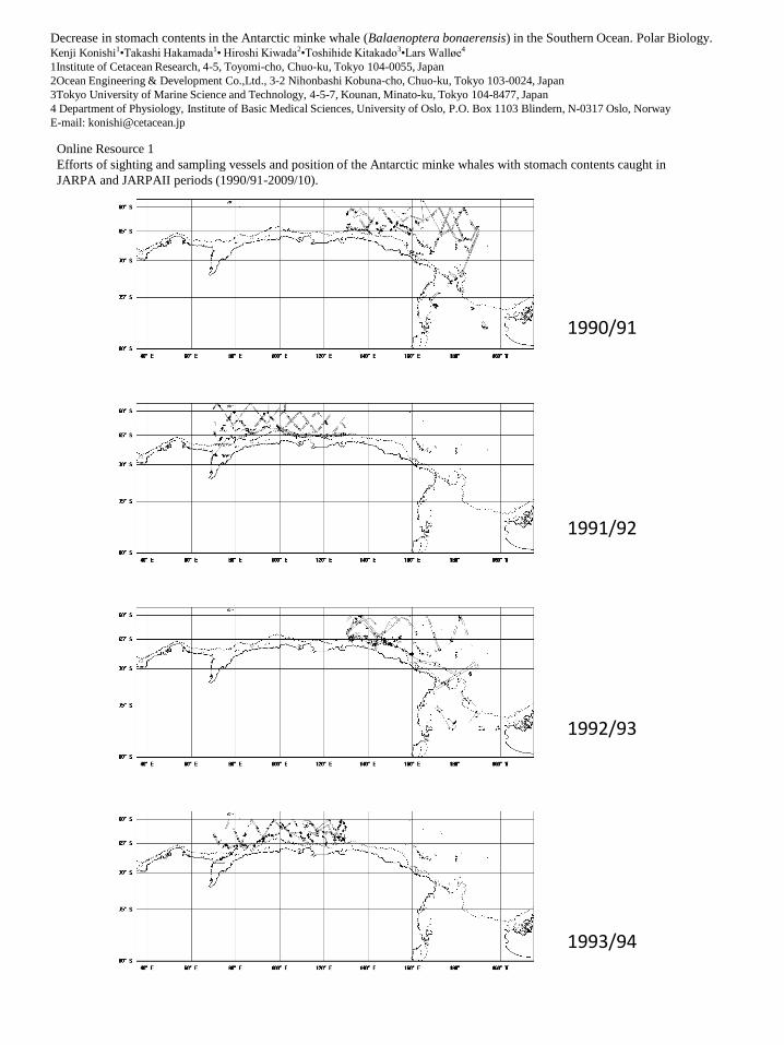
contents caught in JARPA and JARPAII periods (1990/91-2009/10). Grey lines represent search 531

lines and black circles represent sampling positions where whales were sampled. 532

533


List of linear mixed-effects models used in the main analyses with log-transformed stomach content 535

weight (log SCW) as the dependent variable. The covariates in models were selected by an inclusion 536

22

and exclusion process depending on whether the AIC value was smaller than in a previous model 537

(Online Resource 3). 538

539


Results of linear mixed-effects models with log-transformed stomach content weight (log SCW) as the 541

dependent variable. Results are shown for both sexes combined and for males and females separately. 542

The female dataset was divided into two, for lower (<70°S) and higher (>70°S) latitude areas. The 543

Markov chain Monte Carlo (MCMC) method was applied for each model to evaluate and estimate 544

p-values. Delta-AIC = 0 for the minimum AIC in each group of results. 545

546

547

23

Figures 548

Figure 1 549

Map of the study area in the Pacific sector of the Southern Ocean for the 1990/91 to 2009/10 survey 550

seasons. Dots show positions where Antarctic minke whales were sampled during JARPA and JARPA 551

II (blue: male, red: female). The Ross Sea extends into the Antarctic from the Pacific Ocean and its 552

northern limit is at approximately 70°S near Cape Adare. The dotted line shows the 1000m depth 553

contour, which roughly indicates the border between the south continental shelf and offshore waters. 554

The figure at the lower left is a large-scale map showing IWC Management Areas (Donovan 1991), 555

and the black border shows the boundary of the study area. 556

Figure 2 557

Scatterplot of standardized residuals versus fitted values for the linear mixed-effects model 558

LMER24. 559

560

561

Table 1　Data on body length and stomach contents used in the analyses.

All whales mean SD mean SD Nmale 7.96 0.96 17.23 29.55 4407female 8.20 1.20 15.68 30.17 4061

Whales without empty stomachmale 8.06 0.87 26.08 33.03 2912female 8.27 1.13 25.10 34.94 2537

Stomach contents = sieved stomach contents from forestomach

Body length (m) Stomach content weight (kg)

Male Female Male FemaleSurvey Year Average N Average N Average N Average N90/91 26.28 103 31.87 62 21.18 3 15.42 3891/92 30.64 106 30.51 8192/93 37.43 90 33.15 70 21.16 14 17.08 3293/94 36.62 148 29.35 8294/95 21.09 106 24.35 30 22.77 14 27.83 5995/96 33.67 147 21.93 6996/97 26.29 95 30.14 76 40.53 13 36.18 5897/98 31.62 176 28.27 8398/99 29.11 156 24.83 74 - -99/00 27.78 147 27.34 13100/01 21.32 146 23.1 59 19.8 19 18.81 5701/02 27.49 137 17.38 15102/03 26.05 126 25.94 70 27.23 13 45.57 6303/04 25.87 129 24.69 14004/05 18.07 88 18.64 61 30.06 19 21.03 8005/06 21.48 274 23.17 21906/07 29.52 51 20.43 26 19.82 12 26.99 14807/08 15.00 166 19.66 16908/09 16.32 207 19.55 96 31.22 50 27.58 9109/10 29.74 157 24.69 162

Higher Latitude (>70°S)Lower Latitude

Table 3　Results of generalized logistic regression analyses with binary stomach content weight (BI-SCW) as the dependent variable. Data for both sexes were combined.

Models

AIC Year effect SE z-value P valueBI-SCW1 = (Date|Latitude(c))+Year+Local Time+Sex+Body Length 10643 -0.0061 0.0043 -1.421 0.155BI-SCW2 = (Date|Latitude(c))+Year+Local Time+Sex+Longitude(c)+Body Length 10631 -0.0059 0.0045 -1.305 0.192BI-SCW3 = (Date|Latitude(c))+Year+Local Time+Sex+Latitude(c)+Body Length 10608 -0.0038 0.0044 -0.870 0.384

BI-SCW4 = (Date|Latitude(c))+Year+Local Time2+Sex+Body Length+Latitude(c) 10619 -0.0034 0.0044 -0.775 0.438

BI-SCW5 = (Date|Latitude(c))+Year+Local Time+Sex+Body Length3+Latitude(c) 10629 -0.0041 0.0044 -0.943 0.345

BI-SCW6 = (Date2|Latitude(c))+Year+Local Time+Sex+Body Length+Latitude(c) 10608 -0.0038 0.0044 -0.870 0.384

BI-SCW7 = (Latitude|Date(c))+Year+Local Time+Sex+Body Length+Date2+Latitude(c) 10608 -0.0036 0.0044 -0.822 0.411

BI-SCW8 = (Latitude|Date(c))+Year+Local Time+Sex+Body Length+Latitude(c) 10603 -0.0042 0.0044 -0.956 0.339

BI-SCW9 = (Date2|Longitude(c):Year(c))+(Date

2-1|Year(c))+Year+Local Time+Sex+Body Length+Latitude(c) 10515 0.0009 0.0062 0.138 0.891

BI-SCW16 = (Date2|Latitude(c):Longitude(c))+(Date

2-1|Longitude(c)11:Year(c))+Year+Local Time+Sex+Body Length+Latitude(c) 10524 -0.0038 0.0072 -0.530 0.596

BI-SCW17 = (Date2|Latitude(c):Year(c))+(Date

2-1|Longitude(c):Year(c))+Year+Local Time+Sex+Body Length+Latitude(c) 10491 -0.0038 0.0073 -0.518 0.605

(A:B) means A grouped by B.Variable name plus (c) means categorical variableLeft side of vertical bar ‘|’ is fixed effect and right side grouping factor to which the random effect applies.In mixed effects models (GLM3 and GLM4), the symbol ‘:’indicates a crossed random effect, which means grouping factors are crossed.

Coefficient of Year

Table 4 The model evaluation with random and fixed effects for model 24.Random effects:

Groups Name Variance SDLatitude(c):Year(c) Date

2 5.95E-09 7.71E-05

Longitude(c):Year(c) Date2 4.29E-09 6.55E-05

Residual 2.6855 1.6388

Fixed effectsEstimate SE t-value pMCMC

(Intercept) 0.2969 0.4594 0.6460 0.5182Year (1990/91 = 1) -0.0194 0.0063 -3.0840 0.0021Local time (h) -0.1154 0.0064 -17.9730 0.0000Sex (male=1, female=2) -0.1279 0.0487 -2.6270 0.0086Body length (m) 0.3112 0.0236 13.1970 0.0000Variable name plus (c) means categorical variable.

Table 5 Results of linear mixed-effects models with ranked (Ranked SCW) and normal (SCW) stomach content weight.Delta-AIC

Model No. B SE t-value MCMCmean HPD95lowerHPD95upper p by MCMCRanked-SCW model16 23 -16.95 5.692 -2.978 -16.55 -28.085 -5.251 0.0062

model23 21 -17.52 5.155 -3.398 -17.39 -27.390 -6.597 0.0006model24 0 -17.39 5.578 -3.118 -17.28 -27.990 -6.242 0.0016

SCW model16 36 -0.227 0.124 -1.828 -0.222 -0.465 0.039 0.090model23 16 -0.280 0.110 -2.541 -0.267 -0.481 -0.041 0.020model24 0 -0.267 0.122 -2.193 -0.267 -0.508 -0.029 0.029

The Markov chain Monte Carlo (MCMC) technique was applied to each model to evaluate the year effect in the model.Highest posterior density (HPD) interval is calculated for posterior value.

Coefficient MCMC

20°S

40°

60°

80°

40°W 20° 0° 20° 40° 60° 80° 100° 120° 140° 160° 180° 160° 140° 120° 100° 80° 60°

IV I III II V VI

Figure 1

Cape Adare

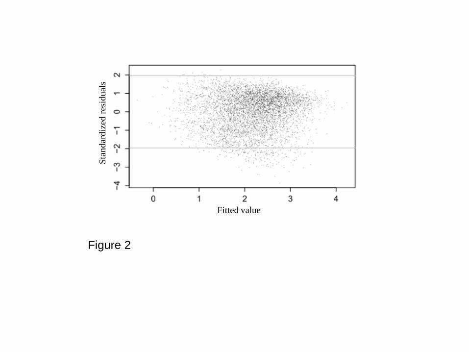
Figure 2

Fitted value

Sta

nd

ard

ized

res

idual

s

1990/91

1993/94

1992/93

1991/92

Decrease in stomach contents in the Antarctic minke whale (Balaenoptera bonaerensis) in the Southern Ocean. Polar Biology. Kenji Konishi1•Takashi Hakamada1• Hiroshi Kiwada2•Toshihide Kitakado3•Lars Walløe4

1Institute of Cetacean Research, 4-5, Toyomi-cho, Chuo-ku, Tokyo 104-0055, Japan

2Ocean Engineering & Development Co.,Ltd., 3-2 Nihonbashi Kobuna-cho, Chuo-ku, Tokyo 103-0024, Japan

3Tokyo University of Marine Science and Technology, 4-5-7, Kounan, Minato-ku, Tokyo 104-8477, Japan

4 Department of Physiology, Institute of Basic Medical Sciences, University of Oslo, P.O. Box 1103 Blindern, N-0317 Oslo, Norway

E-mail: [email protected]

Online Resource 1

Efforts of sighting and sampling vessels and position of the Antarctic minke whales with stomach contents caught in

JARPA and JARPAII periods (1990/91-2009/10).

1994/95

1997/98

1996/97

1995/96

1998/99

2001/02

2000/01

1999/00

2002/03

2005/06

2004/05

2003/04

2006/07

2009/10

2008/09

2007/08

Decrease in stomach contents in the Antarctic minke whale (Balaenoptera bonaerensis) in the Southern Ocean. Polar Biology.


1• Hiroshi Kiwada


3•Lars Walløe

4


Online Resource2　　List of linear mixed-effects models performed in main analyses with log-transformed stomach content weight (log SCW) as dependent variable.

Model No. Models

LMER1 Log-SCW = (Date|Latitude(c))+Year+Local time+Sex+Body length

LMER2 Log-SCW = (Date|Latitude(c))+Year+Local time+Sex+Body length+Longitude(c)

LMER3 Log-SCW = (Date|Latitude(c))+Year+Local time+Sex+Body length+Latitude(c)

LMER4 Log-SCW = (Date|Latitude(c))+Year+Local time2+Sex+Body length+Latitude(c)

LMER5 Log-SCW = (Date|Latitude(c))+Year+Local time+Sex+Body length3+Latitude(c)

LMER6 Log-SCW = (Date2|Latitude(c))+Year+Local time+Sex+Body length+Latitude(c)

LMER7 Log-SCW = (Latitude|Date(c))+Year+Local time+Sex+Body length+Latitude(c)+Date2

LMER8 Log-SCW = (Latitude|Date(c))+Year+Local time+Sex+Body length+Latitude(c)

LMER9 Log-SCW = (Date2|Longitude(c))+Year+Local time+Sex+Latitude(c)+Body length

LMER10 Log-SCW = (Date2|Year(c))+Year+Local time+Sex+Longitude(c)+Latitude(c)+Body length

LMER11 Log-SCW = (Date2|Latitude(c):Longitude(c))+Year+Local time+Sex+Body length

LMER12 Log-SCW = (Date2|Latitude(c):Year(c))+Year+Local time+Sex+Body length

LMER13 Log-SCW = (Date2|Longitude(c):Year(c))+Year+Local time+Sex+Body length

LMER14 Log-SCW = (Date2|Latitude(c):Longitude(c))+(Date|Year(c))+Year+Local time+Sex+Body length

LMER15 Log-SCW = (Date2|Latitude(c):Year(c))+(Date|Year(c))+Year+Local time+Sex+Body length

LMER16 Log-SCW = (Date2|Longitude(c):Year(c))+(Date|Year(c))+Year+Local time+Sex+Body length

LMER17 Log-SCW = (Date2|Latitude(c):Longitude(c))+(Latitude|Latitude(c))+Year+Local time+Sex+Body length

LMER18 Log-SCW = (Date2|Latitude(c):Year(c))+(Latitude|Latitude(c))+Year+Local time+Sex+Body length

LMER19 Log-SCW = (Date2|Longitude(c):Year(c))+(Latitude|Latitude(c))+Year+Local time+Sex+Body length

LMER20 Log-SCW = (Date2|Latitude(c):Longitude(c))+(Latitude|Longitude(c))+Year+Local time+Sex+Body length

LMER21 Log-SCW = (Date2|Latitude(c):Year(c))+(Latitude|Longitude(c))+Year+Local time+Sex+Body length

LMER22 Log-SCW = (Date2|Longitude(c):Year(c))+(Latitude|Longitude(c))+Year+Local time+Sex+Body length

LMER23 Log-SCW = (Date2|Latitude(c):Longitude(c))+(Date|Longitude(c):Year(c))+Year+Local time+Sex+Body length

LMER24 Log-SCW = (Date2|Latitude(c):Year(c))+(Date

2|Longitude(c):Year(c))+Year+Local time+Sex+Body length

Variable name plus (c) means categorical variable.

Left side of vertical bar ‘|’ is random effect and right side grouping factor which the random effect applies.

The symbol ‘:’ indicates a crossed random effect, which means grouping factors are crossed.




4 Department of Physiology, Institute of Basic Medical Sciences, University of Oslo, P.O. Box 1103 Blindern, N-0317 Oslo, Norway

Decrease in stomach contents in the Antarctic minke whale (Balaenoptera bonaerensis) in the Southern Ocean. Polar Biology.


1• Hiroshi Kiwada


3•Lars Walløe

4


Online Resource3 Results of linear mixed-effects models with log-transformed stomach content weight (log SCW) as the dependent variable.Sex combined Delta-AIC Markov chain Monte Carlo (MCMC) technique

Model No. Year effect SE t .value HPD95lower HPD95upper P by MCMCLMER1 155 -0.0264 0.00419 -6.296 -0.0346 -0.0182 0.0001LMER2 172 -0.0243 0.00443 -5.484 -0.0329 -0.0156 0.0001LMER3 147 -0.0246 0.00433 -5.679 -0.0330 -0.0161 0.0001LMER4 176 -0.0242 0.00434 -5.564 -0.0325 -0.0156 0.0001LMER5 168 -0.0250 0.00434 -5.762 -0.0337 -0.0168 0.0001LMER6 144 -0.0245 0.00434 -5.657 -0.0328 -0.0162 0.0001LMER7 172 -0.0248 0.00430 -5.758 -0.0330 -0.0163 0.0001LMER8 152 -0.0253 0.00429 -5.891 -0.0332 -0.0166 0.0001LMER9 132 -0.0253 0.00437 -5.382 -0.0332 -0.0166 0.0001LMER10 60 -0.0201 0.00634 -3.169 -0.0322 -0.0072 0.0022LMER11 105 -0.0217 0.00442 -4.916 -0.0301 -0.0127 0.0001LMER12 54 -0.0207 0.00586 -3.533 -0.0319 -0.0095 0.0002LMER13 21 -0.0204 0.00592 -3.451 -0.0315 -0.0082 0.0008LMER14 38 -0.0175 0.00635 -2.761 -0.0292 -0.004 0.0102LMER15 43 -0.0208 0.00647 -3.212 -0.0332 -0.0077 0.0012LMER16 14 -0.0189 0.00647 -2.926 -0.0312 -0.0047 0.0078LMER17 107 -0.0216 0.00443 -4.884 -0.0305 -0.0128 0.0001LMER18 56 -0.0207 0.00586 -3.526 -0.0319 -0.0087 0.0001LMER19 23 -0.0204 0.00592 -3.451 -0.0323 -0.0087 0.0014LMER20 106 -0.0206 0.00453 -4.545 -0.0296 -0.0118 0.0002LMER21 45 -0.0185 0.00608 -3.041 -0.0304 -0.0066 0.0022LMER22 21 -0.0196 0.00605 -3.233 -0.0311 -0.0073 0.0014LMER23 17 -0.0198 0.00589 -3.355 -0.0317 -0.0084 0.0006LMER24 0 -0.0194 0.00628 -3.084 -0.0315 -0.0071 0.0022

Lower latitudeLMER16 0 -0.0203 0.00673 -3.012 -0.0335 -0.0069 0.0042LMER23 9 -0.0231 0.00589 -3.915 -0.0338 -0.0093 0.0012LMER24 5 -0.0221 0.00629 -3.506 -0.0345 -0.0097 0.0004

MaleLMER16 0 -0.0270 0.00793 -3.400 -0.0423 -0.0107 0.0012LMER23 6 -0.0274 0.00671 -4.079 -0.0409 -0.0135 0.0001LMER24 12 -0.0278 0.00708 -3.924 -0.0421 -0.0136 0.0001

FemaleLMER16 0 -0.0136 0.00923 -1.471 -0.0316 0.0046 0.1528LMER23 11 -0.0132 0.00799 -1.657 -0.0298 0.0019 0.0826LMER24 13 -0.0147 0.00860 -1.708 -0.0310 0.0025 0.0870

Higher latitude LMER16 28 0.0288 0.02234 1.287 -0.0260 0.1289 0.1590LMER23 24 0.0382 0.02345 1.630 -0.0097 0.0922 0.0874LMER24 0 0.0392 0.02424 1.616 -0.0096 0.0961 0.1094

Lower latitude LMER16 0 -0.0215 0.00957 -2.244 -0.0407 -0.0025 0.0298LMER23 2 -0.0233 0.00880 -2.644 -0.0410 -0.0059 0.0116LMER24 2 -0.0236 0.00887 -2.664 -0.0415 -0.0056 0.0104

Bold type shows the three models with the lowest AIC values for both sexes combined. These models were run for separate male and female datasets.The Markov chain Monte Carlo (MCMC) technique was applied to each model to evaluate the year effect in the model.

Highest posterior density (HPD) interval is calculated for posterior value.

Coefficient

The female dataset was divided into two different latitudinal groups because of the wide latitudinal distribution of female whales (higher (Ross Sea) andlower latitudes, split at 70°S).




4 Department of Physiology, Institute of Basic Medical Sciences, University of Oslo, P.O. Box 1103 Blindern, N-0317 Oslo,

decrease in stomach contents in the antarctic minke whale

Documents