Decoupled farm payments and the Role of BaseUpdating under uncertainty

Arathi Bhaskar John C. BeghinIowa State University Iowa State University

And University of Sydney

October 2007

Abstract

In the context of the U.S farm policy, this paper analyzes the effect that expectationsabout base updating in future policies has on a farmer’s acreage decision in the presence ofprice, yield and policy uncertainty. We consider a risk neutral farmer producing a single cropwhose income consists of market revenue and government payments. We consider two policyregimes. Decisions made in the current policy regime are linked to government payments inthe future policy regime through the possibility of a base update in the future regime. Thereis policy uncertainty about the possibility of a base update being allowed in the future. Wecombine stochastic dynamic programming with present value calculations to link currentacreage decisions to future program payments. The average optimal planted acreage is non-decreasing in the subjective probability of the future base update. The maximum percentageincrease in the average optimal planted acreage conditional on price and the certainty of thefuture base update occurring is 6%.

1. Introduction

The Uruguay Round Agreement on Agriculture (URAA) of the World Trade Organization

(WTO) in 1994 was the first time that a major step was taken towards reducing the trade dis-

tortions caused by domestic agricultural subsidies. Domestic subsidies were classified into three

categories or “boxes” according to the level of distortion that they caused. The amber-box con-

tains the most distorting subsidies and are therefore required to be limited in use. The blue-box

payments also cause some distortion but are required to be production limiting. The green-box

contains subsidies that cause no or minimal distortion. The subsidies in the blue- and green-boxes

are currently excluded from all WTO disciplines. Decoupled payments fall under the green-box

and are defined as payments that are financed by taxpayers, are not related to current produc-

tion, factor use, or prices, and for which eligibility criteria are defined by a fixed, historical base

period. Since there are no restrictions on their use they have come to play an important role in

providing support to farmers especially in industrialized countries.

Recently though, green-box subsidies, especially decoupled payments, have come under

scrutiny. The WTO rulings against the United States in the cotton dispute (WTO (2004), WTO

(2005)) has brought the direct payments under the spotlight. There is an ongoing debate over the

impact that decoupled payments have on farmer decisions. The different “coupling” mechanisms

of decoupled payments have been analyzed in the literature.

Hennessy (1998) and Sckokai and Moro (2002) find that in the presence of uncertainty, de-

coupled payments have wealth and insurance effects with the insurance effect dominating the

wealth effect. Roe, Somwaru and Diao (2003) find that in the presence of segmented capital mar-

kets, decoupled payments have small effects that last only in the short run. Goodwin and Mishra

(2006) examine the effect of decoupled payments on farmers’ acreage decision. For the corn belt

1

region, they find that decoupled payments have a small but positive effect on acreage of corn and

soybeans. They also find that these payments lead to less land idling. Empirical results of El-Osta

et al. (2004) and Ahearn et al. (2006) indicate that decoupled payments influence labor allocation

decisions. Goodwin et al. (2003a), Goodwin et al. (2003b) and Roberts et al. (2003) find that de-

coupled payments increase land rents and land values as they are non-stochastic payments based

on land.

In the context of U.S. farm policy, our paper focuses on how a farmer’s expectations regarding

future decoupled payments influence their decisions. The 2002 FSRI Act in the United States

allowed base updating. Also some new commodities (soybeans, other oilseeds, and peanuts)

were added under the direct payment program. These features create potential incentives for

farmers to increase production, possibly creating a link between future payments and current

production. While the 1996 FAIR Act did not allow for base updating, the 2002 FSRI Act did

allow for base updating. If farmers expect that future Farm Bills might allow base updating, then

they link an increase in current acreage to higher future government payments that are paid on

base acres. Thus base updating may create incentives to expand production under the 2002 FSRI

Act. On the other hand the effect of the uncertainty regarding future policies might depress the

incentives associated with base updating. Uncertainty about the different payment rates could

also influence producer decisions such as the area to be planted and input use. Sumner (2003),

McIntosh et al. (2006) and Coble and Hudson (2007) have analyzed the effect of expectations

about a future opportunity to update base. Complementary to Sumner (2003), McIntosh et al.

(2006) and Coble and Hudson (2007), our approach formalizes and quantifies the influence of

expected payments under future policy which might allow a base update on acreage decisions

under current policy.

2

We analyze the impact of base updating on a farmer’s acreage decision in the presence of

price, yield and policy uncertainty. We consider a risk neutral farmer producing a single crop

whose income consists of market revenue and government payments. Three government pay-

ments are considered; direct payments (DP), counter-cyclical payments (CCP) and loan de-

ficiency payments (LDP). The farmer makes acreage planting decisions in the current policy

regime, (2002-06) not knowing what policies will be in place in the future policy regime (the

duration of the 2007 Farm Bill). If base updating is allowed in the future regime, then the new

base acreage for DP and CCP, is considered to be the average of the planted acreage in the cur-

rent regime. The subjective beliefs of the farmer formed under the current Farm Bill, regarding

a future base update occurring, (δ), is discretized into five values, starting from 0 (no update) to

1 (certain update) in increments of 0.25. The farmer’s problem is to maximize the present value

of profits by choosing acreage during 2002-06 while taking into account expected future policy

changes, including the possibility of a base update. Thus the farmer cares not only about his/her

current income but also about the future stream of income.

The solution to the model provides the optimal planted acreage for each of the years 2002-06

and for each value of the subjective probability about the future base update. The results are

presented in terms of the average of the optimal planted acreage, A, over 2002-06. Under cer-

tainty that there is no future base update, this value is driven entirely by market conditions and

current government programs, and establishes a “business as usual” baseline. Under certainty

that there will be an opportunity to update base, this value is driven by market conditions and the

expectation that base updating will be allowed for sure. A is then the new base acreage for DP

and CCP. Similarly for intermediate values of δ, A is driven by the varying degrees of conviction

regarding the possibility of a future base update. A is weakly increasing in δ. We then compute

3

the percent increase in A for δ > 0 relative to δ = 0 to quantify the supply expansion effect of an

expected base update. The results indicate that the maximum percentage increase in A is 6%. We

also look into alternate assumptions regarding policy parameters to investigate the robustness of

our main result. The paper is organized as follows. In the next section the literature on decoupled

payments in the United States is reviewed. Section 3 discusses the model, section 4 describes the

numerical analysis, section 5 presents the results and finally section 6 concludes.

2. Model

We follow Duffy and Taylor (1994) in formulating the acreage optimization problem for a risk

neutral farmer. The farmer produces a single crop, corn, and faces price and yield uncertainty,

with price and yield being negatively correlated. She earns income from the sale of her crop

and government payments. Three government payments are considered; LDPs, DPs and CCPs.

Of the three programs, DPs and CCPs depend on historical base acreage and historical yields1.

CCPs are triggered by low prices, as are loan deficiency payments. Thus updating base acreage

or historical yields affect the DPs and CCPs. The per-period profit of the farmer can be written

as:

πt = PtYtAt+max(LR−(Pt−0.26), 0)YtAt+0.85D∗BA∗Yd+0.85∗max(CR, 0)∗BA∗Yc−TC(At),

(1)

where Pt is the stochastic price, Yt is the stochastic yield, At is the current acreage, LR is the

loan rate, Pt− 0.26 represents the posted county average price2, D is the DP rate, CR is the CCP

1In the years 1998-2001 farmers received payments termed as the Market Loss Assistance (MLA) paymentsbecause of low prices. These ad-hoc payments were made permanent in the 2002 FSRI Act and called the CCPs.

2Babcock and Hart (2005) find that on average the posted county average price (used for computing LDP rate) isless than the season average price by 0.26 in the case of corn.

4

rate which equals TP −D−max(Pt, LR), where TP is the target price and TC is the total cost

of production which is a function of current acreage. BA is the base acreage for the duration of

the 2002 FSRI Act, and Yd and Yc are program yields for the DPs and CCPs respectively. Thus

profit, πt, is a function of Pt, Yt and At.

The farmer maximizes profits with respect to acreage over the period 2002-06 while taking

into account the possibility of a base update being allowed in the 2007 Farm Bill. This implies

that the farmer maximizes the expected present value of profits:

maxAt

E

[4∑

t=0

βtπt(At, Pt, Yt) + β5(δV B + (1− δ)V NB)

], (2)

where β is the discount factor and δ ∈ [0, 1] captures the farmer’s subjective probability regarding

an opportunity to update base in the 2007 Farm Bill. Five values of δ have been considered to

capture the varying degrees of conviction that the farmer has regarding the future policy changes.

δ = 0 implies that the farmer is certain that base update will not be allowed in the 2007 Farm

Bill. On the other hand δ = 1 implies that the farmer is certain that base updating will be allowed

in the 2007 Farm Bill. V B and V NB represent the future income stream for the farmer.

V B is the value function for the stochastic dynamic programming (SDP) problem associated

with base updating and other policy changes (SDPV B). V NB is the value function for the SDP

problem associated with no base updating in the 2007 Farm Bill (SDPV NB). Thus the farmer is

weighing the future income stream with δ. As the farmer’s beliefs about the expected base update

changes, land allocation decisions in 2002-06 are affected. Equation (2) also provides the link

between acreage decisions in 2002-06 with future farm payments. This is because under base

updating, the new base (which is the average of the acreage planted in 2002-06) affects V B.

5

The two SDP problems are solved for a five-year time horizon, representing the years 2007-

2011, and a discrete state and control space. The control or decision variable is the current

acreage, At, which is discretized into r values. The stochastic state variables are price and yield.

Both the variables are discretized into t and s number of states respectively. Additionally, for

SDPV B, the state space also includes all the possible values for the new base. Since price and

yield are stochastic, there is a probability associated with the realization of each of the possible

t price and s yield states. The probability transition matrix, which is a (t ∗ s) × (t ∗ s) matrix

contains these probabilities. An element pi,j,k,l of the probability transition matrix represents the

probability of moving from a current price of i and a yield of j to a price of k and yield of l in

the next period. We rewrite (2) as:

maxAt

4∑t=0

t∑k=1

s∑l=1

βtP i,j,k,l−→πt(At, Pt, Ynt) + β5

t∑k=1

s∑l=1

P i,j,k,l(δ ∗ −−→V B + (1− δ) ∗ −−−→V NB). (3)

The two SDP problems are:

V Bt(Pt, Ynt, BA′) =

maxAt

[∑tk=1

∑sl=1 P i,j,k,lπt(Pt, Ynt, At, BA′) + β

∑tk=1

∑sl=1 P i,j,k,lV Bt+1(Pt+1, Ynt, BA′)

],

t = 1, 2, ...5.

(4)

6

V NBt(Pt, Ynt) = maxAt

[∑tk=1

∑sl=1 P i,j,k,lπt(Pt, Ynt, At) + β

∑tk=1

∑sl=1 P i,j,k,lV NBt+1(Pt+1, Ynt)

],

t = 1, 2, ...5,

(5)

where BA′ is the new base acreage for the DPs and the CCPs for 2007-2011 and is the average

of the acreage planted during 2002-06. The option of not updating is also included amongst all

the possible base values considered. Here BA′ is treated as an endogenous state variable.

3. Numerical Solution

The numerical analysis is carried out at a national level using national season average price

and yield. We also take into account payment limitations while computing profits3. We assume

that the farmer receives DPs and CCPs on a base acreage of 1000 acres. Yd = 118 bu/acre is

the same as the program yield established in the Food, Agriculture, Conservation, and Trade

(FACT) Act of 19904. Farmers were given the opportunity to update their program yields for the

CCPs. The following two methods were allowed: (i) 93.5% of the 1998-2001 average yield or,

(ii) Yd + 70% ∗ ((1998− 2001 average) −Yd). If farmers choose not to update their yield then Yd

would be used. With Yd = 118 bu/acre, method (ii) results in the highest Yc and equals 130.48

bu/acre. D = 0.28 is assumed to remain the same for the 2007 Farm Bill.

The functional form considered for the total cost, TC(At), is F + bAt + cA3t where F is the

fixed cost and b and c are constants. Given F , we calibrate b and c for a 1000 acre farm using the

profit maximization condition and the acreage price elasticity 5.

3The 2002 Farm Act sets payment limits at $40,000 per person per fiscal year for DPs, at $65,000 for CCPs andat $75,000 for LDPs. In our analysis the payment limitations are binding only for LDPs when LR > Pt − 0.26

4The 2002 FSRI Act did not allow a yield update for DPs.5We use an estimate of acreage price elasticity equal to 0.412 (Lin et al. (1996)).

7

Both the price and yield state variables are discretized into eight values each, yielding a total

of 64 states. At is discretized into eight values, starting at 900 acres with increments of 50 acres.

Since the farmer can choose any one of the eight acreage choices in each of the five years, 2002-

06, the total number of new base values is large (32,768). Thus the total number of states for

SDPV B is even larger (32, 768 ∗ 64 = 20, 97, 152). For SDPV NB the total number of states

equal 64.

The elements in the probability transition matrix are derived from the joint distribution of

price and yield. We assume that price and yield follow a bivariate normal distribution6 with

negative correlation between price and yield. To compute the transition matrix, we also need to

estimate the first and second moments of price and yield.

Expected yield depends on a trend variable and expected price depends on lagged price.

Equations for expected price and yield are estimated as seemingly unrelated regressions using

time series data for the period 1980-2005 (price and yield data were obtained from the National

Agricultural Statistics Service (NASS)). Nominal prices have been deflated to 2005 prices using

the GDP price deflator. The results of the estimation are obtained as7:

EYt = 95.80 + 1.95 ∗ T − 29.06 ∗Dy (6)

where T is trend and Dy is a dummy variable which is equal to 1 for 1988 and 0 otherwise. The

variance σ2Y was estimated as 115.31.

EPt = 0.83 + 0.65 ∗ Pt−1 + 1.35 ∗Dp (7)6The Shapiro-Wilk test was used to test whether the price and yield distributions follow a normal distribution.

The null hypothesis of normality could not be rejected at the 5% level of significance7All coefficients are statistically significant at the 5% level of significance.

8

where Dp is a dummy variable which is equal to 1 for 1983 and 1995 and 0 otherwise. The vari-

ance, σ2P was estimated as 0.162. The dummy variables are employed for observations identified

as outliers8.

Yield is known to have an upward trend and it is important to capture this in the per-period

profit. To capture the trend in yield in (1) and to allow the yield states to be constant over

time, we transform yield to a standard normal variable while calculating the probability transition

matrix. Actual yield in a particular year, t, can be written as a function of the normalized yield

as Yt = Yn ∗ σY + E(Yt). Therefore the yield states are specified in terms of Yn: -1.75, -

1.25, -0.75, -0.25, 0.25, 0.75, 1.25 and 1.75. The following price states ($/bu) were chosen

to represent the probable range of prices: 1.625, 1.875, 2.125, 2.375, 2.625, 2.875, 3.125 and

3.375. Probabilities are then derived from the joint distribution of price and normalized yield9.

The probability transition matrix in our problem is driven by the price states. For example, the

probability of attaining any one of the 64 states starting from the previous yield state of -1.75

and previous price state of 1.625 is equal to the probability of attaining any one of the 64 states

starting from the previous yield state of 0.25 and previous price state of 1.625. This is because

the transition to any state in the next period depends only on the current price state via (7).

Yield in the next period is not affected by the yield in the current period. While calculating the

probability transition matrix we also take into account the truncation caused by the loan rate on

8An alternate specification was also considered by deleting observations corresponding to the outlier years. Hu-ber’s M estimation was also used to identify outliers. In this case only outliers in the price series were detected,corresponding to the same two years. Two specifications of the EYt and EPt equations were estimated, one with adummy variable for price and the second by deleting the observations for the outlier years. Finally we also estimatedthe two equations without treating for outliers. The results are robust to all the other specifications used.

9An element of the transition matrix, pi,j,k,l =∫ k

k

∫ l

lf(P, Yn; ρ)dYndP , where f(·) is the probability density

function of a bivariate normal distribution and ρ is the correlation coefficient between price and yield. Price statek ∈ (k, k) and yield state l ∈ (l, l). The price and yield states have been constructed as mid-points of intervals.The first price interval starts at $ 1.5/bu and goes upto a maximum of $ 3.5/bu in increments of 25 cents. The firstnormalized yield interval starts at -2 bu/acre and goes upto a maximum of 2 bu/acre in increments of 0.5 bu/acre.

9

the joint distribution of price and yield10. We use numerical integration to compute the probability

transition matrix.

SDPV B and SDPV NB are solved using backward recursion. The terminal value functions,

V B6 and V NB6 are initially assumed to be zero. We then solve for V B1 and V NB1 and substi-

tute these back as V B6 and V NB611 and solve again for V B1 and V NB1. These are the values

that enter in (3). Finally we calculate the present value of expected profits as defined in (3) for

each possible base value. The farmer maximizes the expected present value over all base values.

In the discussion above, we assume that the policy parameters in the 2002 and 2007 Farm

Bills remain the same and the farmer is faced only with uncertainty about the expected future

base update (denoted as case (i)). We also consider two other cases with respect to the expected

policy changes in the 2007 Farm Bill. These also include the uncertainty regarding an expected

base update. Under case (ii), the loan rate and the target price are reduced over the period 2007-

11 and there is no uncertainty regarding these rates. Under case (iii), the loan rate and the target

price are reduced over the period 2007-11 and there is uncertainty regarding the reduction in the

rates as well as base updating. The reduced rates for 2007-2011 are listed in Table 212. We solve

SDPV B and SDPV NB for case (ii) in a similar way as we did for case (i). Case (iii) is a combi-

nation of case (i) and case (ii), i.e. it is a combination of V B from case (ii) and V NB from case

(i). Thus for δ = 0, the expected present value of profit is equal under cases (i) and (iii); and for

δ = 1, the expected present value of profit is equal under cases (ii) and (iii).

10Calculation of the truncated mean and variance of prices and yields is based on (Greene 2002, chap. 22).11We do this to get an estimate of expected future income.12The reduced rates are taken from FAPRI (2005). These rates have been reduced to meet the October 2005 U.S

proposal in the WTO agricultural negotiations.

10

4. Results

Since the transition matrix depends entirely on the price states, the final payoffs are are also

entirely dependent on the price states. For example the payoff from a yield state of -1.75 and

price state of 1.625 is equal to the payoff attained from a yield state of 0.25 and a price state of

1.625. We therefore present the results for the eight price states. The solution to the farmer’s

problem is conditional on the price state in the year 2001 and the farmer’s subjective probability

about the expected base update. The solution to the problem is the optimal planted acreage to be

planted in each of the years 2002-2006.

The supply response is measured in terms of the average of the optimal planted acreage for

the years 2002-06, A. We present A for each of the price states and all values of δ in Table 3 for

case (i). With a few exceptions, A strictly increases as δ increases. For price state $1.625/bu and

δ = 0.25 and 0.5, price state $1.875/bu and δ = 0 and 0.25 and price state $2.125/bu and δ = 0, it

is optimal for the farmer not to make any changes to the acreage, i.e., the farmer should continue

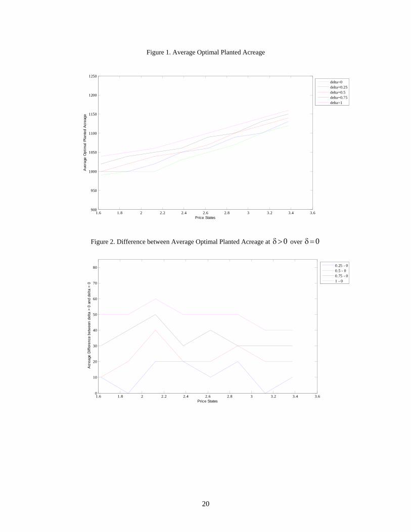
to plant 1000 acres in each of the years 2002-06. This result is driven by low prices. Figure 1

plots A against the price states for each value of δ. As δ increases, A shifts outwards. Figure

2 measures the supply response to the expected base update. When δ = 0, A is determined by

market conditions and farm programs in place in 2002-06. Thus, A at δ = 0 is the benchmark to

which we compare the A for δ > 0. A|δ>0 − A|δ=0 measures the supply effect13 of the expected

base update. We also compute the percent increase in A for δ > 0 relative to δ = 0. These

are presented in Table 4. For price states, $1.625, $1.875 and $2.125/bu farmers receive both

DPs and CCPs. There is therefore a link between an expected base update and future DPs and

CCPs. The maximum percent increase is 6% for $2.125/bu and δ = 1. It decreases to 4% as

13Here supply effect represents the expansion in acreage when δ increases.

11

δ decreases to 0.5. For $2.125/bu, the percent increase is the highest for all values of δ > 0.

For price states, $2.375, $2.625, $2.875, $3.125 and $3.375, only DPs are made to farmers and

therefore the results for these price states captures the supply effect of the expected base update

for the “decoupled” DPs. Averaged over the five price states, the percent increase in acreage for

δ = 1 is about 4%. When δ falls to 0.5 it decreases to less than 3%.

Under cases (ii) and (iii), the expected present value of profits are lower compared to case (i).

Also for δ = 1 the expected present value is equal for cases (ii) and (iii); for δ = 0, the expected

present value is equal for cases (i) and (iii). Even though the expected payoffs are lower under

cases (ii) and (iii), there is no change in A. This can be attributed to the fact that the reduction in

the payoffs are not large enough to affect the optimal planted acreage.

We also conduct sensitivity analysis for a change in the acreage price elasticity. Results for

an acreage price elasticity of 0.6 are presented in Tables 5 and 6, and Figures 3 and 4. A increases

for all values of δ. Comparing Tables 4 and 6 shows that increasing the acreage price elasticity

does not have dramatic effects on the acreage supply response to the expected base update. The

effect of an expected base update on current acreage remains small.

5. Conclusion

DPs in the 2002 FSRI Act fulfill many of the eligibility criteria of the decoupled payments

as defined in the URAA. But the planting restrictions imposed on base acres and the base update

allowed in the 2002 FSRI Act disqualify these payments as green-box. The United States is

negotiating to place the DPs in the green-box in the Doha round of the WTO.

There is a voluminous literature analyzing the effects of decoupled payments in the United

States (the PFC payments in the 1996 FAIR Act and the DPs in the 2002 FSRI Act) on farmer

12

decisions. The literature on decoupling indicates that decoupled payments do have coupling

effects, albeit small in magnitude, with the exception of the effect on land values.

Our paper adds to the current literature on the role of base updating by presenting a formalized

model to examine the role of base updating in a farmer’s decision making process. We analyzed

the effect of an expected base update in the 2007 Farm Bill on a farmer’s current acreage decision,

in the presence of price and yield uncertainty. Price and yield are discretized into eight states each,

to approximate the uncertainty faced by the farmer. We measure the change in acreage supply

response to an expected base update as the farmer’s expectation of the future update changes,

which is captured by δ ∈ [0, 1]. We find that the maximum percent increase in the average of

the optimal planted acreage over 2002-06 is 6% conditional on price = $2.125/bu and δ = 1.

At prices = $1.625, $1.875 and $2.125/bu, CCPs are positive and therefore any opportunity to

update base increases both the DPs and the CCPs. The average of the optimal planted acreage is

weakly increasing in δ.

Our results indicate that expectations about future policies influence producer decisions.

These results have important policy implications for the WTO negotiations in the Doha round.

At present, the proposals of the U.S. and EU, or even the Harbinson proposal for the Doha round

do not contain any changes to the green-box payments. But our results suggest that the green-box

criteria for decoupled payments must be made very clear, with no room for ambiguities. It should

be made clear that allowing base update or including new commodities in the program violate the

criteria of decoupled payments being paid on fixed historical base, although this effect is small.

Once a base update is allowed, decoupled payments should no longer be classified as green-box

payments.

Lastly, we would like to point out that our analysis is conducted in the short-run. In the

13

long-run, costs are flatter and we expect the acreage response to be higher. Therefore we expect

a larger acreage expansion as the probability of a future base update increases. Our analysis is

conducted for a single program crop, corn. We therefore consider our results to be an upper

bound on acreage expansion. A possible avenue of future research could be to extend this model

to include two crops.

14

ReferencesAhearn, M., El-Osta, H., and Dewbre, J. (2006). The impact of coupled and decoupled govern-

ment subsidies on off-farm labor participation of U.S farm operators. 88(2). American Journalof Agricultural Economics.

Babcock, B. and Hart, C. (2005). How much “safety” is available under the U.S. proposal to theWTO? Briefing Paper, Center for Agricultural and Rural Development.

Coble, K.H, M. J. and Hudson, M. (2007). Decoupled farm payments and expectations for baseupdating. Working paper, Mississippi State Department of Agriculture Economics.

Duffy, P. and Taylor, R. (1994). Effects on a corn-soybean farm of uncertainty about the futureof farm programs. American Journal of Agricultural Economics, 76:141–152.

El-Osta, H., Mishra, A., and Ahearn, M. (2004). Labor supply by farm operators under “decou-pled” farm program payments. Review of Economics of the Household, 2:367–385.

FAPRI (2005). Potential impacts on U.S. agriculture of the U.S. October 2005 WTO proposal.Food and Agricultural Policy Research Institute, University of Missouri-Columbia Report No.16-05.

Goodwin, B. and Mishra, A. (2006). Are “decoupled” farm program payments really decoupled?An empirical evaluation. American Journal of Agricultural Economics, 88:73–89.

Goodwin, B., Mishra, A., and Ortalo-Magne, F. (2003a). Explaining regional differences inthe capitalization of policy benefits into agricultural land values. In: Government Policy andFarmland Markets, pages 97–114. Edited by C.B. Moss and A. Schmitz, Iowa State Press.

Goodwin, B., Mishra, A., and Ortalo-Magne, F. (2003b). What’s wrong with our models ofagricultural land values? American Journal of Agricultural Economics, 85:744–752.

Greene, W. (2002). Econometric Analysis. Prentice Hall, 5 edition.

Hennessy, D. (1998). The production effects of agricultural income support policies under un-certainty. American Journal of Agricultural Economics, 80(1).

Lin, W., Westcott, P., Skinner, R., Sanford, S., and D., T. (1996). Supply response under the 1996Farm Act and implications for the U.S. field crops sector. Economic Research Service, UnitedStates Department of Agriculture.

McIntosh, C., Shogren, J., and Dohlman, E. (2006). Supply response to counter-cyclical pay-ments and base acre updating under uncertainty: An experimental study. Preliminary Draft.

Roberts, M., Kirwan, B., and Hopkins, J. (2003). Incidence of government program paymentson land rents: The challenges of identification. American Journal of Agricultural Economics,85(3):762–769.

15

Sckokai, P. and Moro, D. (2002). Modelling the CAP arable crop regime under uncertainty. Paperpresented at the American Agricultural Economics Association Annual Meeting, Long Beach,California.

Sumner, D. (2003). Implications of the us farm bill of 2002 for agricultural trade and tradenegotiations. Australian Journal of Agricultural and Resource Economics, 47:99–122.

WTO (2004). Panel report (http://www.wto.org/english/tratop e/dispu e/cases e/ds267 e.htm).

WTO (2005). Appelate body report (http://www.wto.org/english/tratop e/dispu e/cases e/ds267 e.htm).

16

Table 1: Model Parameters

β 0.95BA 1000 acresYd 118 bu/acreYc 130.48 bu/acreF $ 208230b -23.47c 0.00012

Table 2: Loan rates and Target price for 2002- 2011

2002 2003 2004 2005 2006LR 1.98 1.98 1.95 1.95 1.95TP 2.60 2.60 2.63 2.63 2.63

2007 2008 2009 2010 2011LR 1.91 1.86 1.82 1.78 1.74TP 2.59 2.56 2.52 2.48 2.45

17

Table 3: Average Optimal Planted Acreageδ

Price State 0 0.25 0.5 0.75 11.625 990 1000 1000 1020 10401.875 1000 1000 1020 1040 10502.125 1000 1020 1040 1050 10602.375 1030 1050 1050 1060 10802.625 1050 1060 1070 1090 11002.875 1070 1090 1100 1100 11203.125 1100 1100 1120 1130 11403.375 1120 1130 1140 1150 1160

Table 4: Percent change in A relative to δ = 0δ

Price State 0.25 0.5 0.75 11.625 1.01 1.01 3.03 5.051.875 0.00 2.00 4.00 5.002.125 2.00 4.00 5.00 6.002.375 1.94 1.94 2.91 4.852.625 0.95 1.90 3.81 4.762.875 1.87 2.80 2.8 4.673.125 0.00 1.82 2.73 3.643.375 0.89 1.79 2.68 3.57

18

Table 5: Average Optimal Planted Acreage with Acreage Price Elasticity of 0.6δ

Price State 0 0.25 0.5 0.75 11.625 1000 1010 1030 1050 10701.875 1010 1030 1050 1070 10902.125 1040 1050 1070 1090 11102.375 1060 1080 1100 1120 11302.625 1100 1110 1130 1140 11602.875 1130 1140 1160 1180 11903.125 1160 1180 1190 1210 12203.375 1190 1210 1220 1230 1250

Table 6: Percent change in A relative to δ = 0 with Acreage Price Elasticity of 0.6δ

Price State 0.25 0.5 0.75 11.625 1.00 3.00 5.00 7.001.875 1.98 3.96 5.94 7.922.125 0.96 2.88 4.81 6.732.375 1.89 3.77 5.66 6.602.625 0.91 2.73 3.64 5.452.875 0.88 2.65 4.42 5.313.125 1.72 2.59 4.31 5.173.375 1.68 2.52 3.36 5.04

19

20

Figure 1. Average Optimal Planted Acreage

1.6 1.8 2 2.2 2.4 2.6 2.8 3 3.2 3.4 3.6900

950

1000

1050

1100

1150

1200

1250

Price States

Ave

rage

Opt

imal

Pla

nted

Acr

eage

delta=0delta=0.25delta=0.5delta=0.75delta=1

Figure 2. Difference between Average Optimal Planted Acreage at 0>δ over 0=δ

1.6 1.8 2 2.2 2.4 2.6 2.8 3 3.2 3.4 3.60

10

20

30

40

50

60

70

80

Price States

Acr

eage

Diff

eren

ce b

etw

een

delta

> 0

and

del

ta =

0

0.25 - 00.5 - 00.75 - 01 - 0

21

Figure 3. Average Optimal Planted Acreage with Acreage Price Elasticity of 0.6

1.6 1.8 2 2.2 2.4 2.6 2.8 3 3.2 3.4 3.6900

950

1000

1050

1100

1150

1200

1250

Price States

Ave

rage

Opt

imal

Pla

nted

Acr

eage

delta=0delta=0.25delta=0.5delta=0.75delta=1

Figure 4. Difference between Average Optimal Planted Acreage at 0>δ over 0=δ with Acreage Price Elasticity of 0.6

1.6 1.8 2 2.2 2.4 2.6 2.8 3 3.2 3.4 3.60

10

20

30

40

50

60

70

80

Price States

Acr

eage

Diff

eren

ce b

etw

een

delta

> 0

and

del

ta =

0

0.25 - 00.5 - 00.75 - 01 - 0