arX

iv:0

810.

0003

v1 [

astr

o-ph

] 1

Oct

200

8

Mon. Not. R. Astron. Soc. 000, 000–000 (0000) Printed 30 May 2018 (MN LATEX style file v2.2)

Deconstructing Baryon Acoustic Oscillations:

A Comparison of Methods

Anaıs Rassat1, Adam Amara2, Luca Amendola3, Francisco J. Castander4,

Thomas Kitching5, Martin Kunz6,7, Alexandre Refregier1, Yun Wang8, Jochen Weller91IRFU-SAP, Service d’Astrophysique, CEA-Saclay, F-91191 Gif sur Yvette Cedex, France.2Institute for Astronomy, ETH Hoenggerberg Campus, Physics Department, CH-8093 Zurich, Switzerland.3INAF - Osservatorio Astronomico di Roma, Via Frascati 33, 00040 Monte Porzio Catone, Roma, Italy.4Institut de Ciencies de l’Espai (IEEC/CSIC), Campus UAB, 08193 Bellaterra, Barcelona, Spain5University of Oxford, Department of Physics, Denys Wilkinson Building, Keble Road, Oxford, OX1 3RH, United Kingdom.6Institute for Theoretical Physics, University of Geneva, 24, Quai Ernest-Ansermet, CH-1211 Geneve 4, Switzerland.7Department of Physics and Astronomy, University of Sussex, Brighton, East Sussex BN1 9QH, United Kingdom.8Dept. of Physics & Astronomy, The University of Oklahoma, 440 W. Brooks St., Norman, OK 73019, USA.9Physics & Astronomy, University College London, Gower Street, London WC1E 6BT, United Kingdom.

Accepted xxx. Received xxx; in original form xxx

ABSTRACTThe Baryon Acoustic Oscillations (BAOs) or baryon wiggles which are present in thegalaxy power spectrum at scales 100− 150h−1Mpc are powerful features with whichto constrain cosmology. The potential of these probes is such that these are nowincluded as primary science goals in the planning of several future galaxy surveys.However, there is not a uniquely defined BAO Method in the literature but a range ofimplementations. We study the assumptions and cosmological performances of threedifferent BAO methods: the full Fourier space power spectrum [P (k)], the ‘wigglesonly’ in Fourier space and the spherical harmonics power spectrum [C(ℓ)]. We contrastthe power of each method to constrain cosmology for two fiducial surveys taken fromthe Dark Energy Task Force (DETF) report and equivalent to future ground and spacebased spectroscopic surveys. We find that, depending on the assumptions used, thedark energy Figure of Merit (FoM) can change by up to a factor of 35 for a given fiducialmodel and survey. We compare our results with the DETF implementation and, discussthe robustness of each probe, by quantifying the dependence of the FoM with thewavenumber range. The more information used by a method, the higher its statisticalperformance, but the higher its sensitivity to systematics and implementations details.

1 INTRODUCTION

In the early Universe, just before recombination, fluctua-tions in the coupled baryon-photon fluid were subject totwo competing effects: attractive gravity and repulsive pres-sure. These two effects are expected to produce a seriesof acoustic peaks - dubbed Baryon Acoustic Oscillations(BAOs) - in both the Cosmic Microwave Background (CMB)(Sunyaev & Zeldovich 1970; Peebles & Yu 1970) and thematter power spectra (Eisenstein & Hu 1999).

These features have been observed in the CMBtemperature-temperature power spectrum using data fromseveral years of the Wilkinson Microwave Anisotropy Probe(WMAP) data (for the latest measurements see Nolta et al.2008). As galaxy surveys cover increasingly larger volumes,they too can probe the scales on which the BAOs are pre-dicted. Recently these have been observed in the Sloan Dig-ital Sky Survey (SDSS) (Eisenstein et al. 2005; Hutsi 2006a;

Percival et al. 07 a) and the 2 degree Field Galaxy Survey(2dFGS) (Percival et al. 07 b).

The scale of the oscillations provides a standardruler and has been used to constrain dark energy pa-rameters (Eisenstein et al. 2005; Amendola et al. 2005;Wang & Mukherjee 2006; Wang 2006; Percival et al. 07 a,b;Ichikawa & Takahashi 2007) as well as neutrinos masses(Goobar et al. 2006) and even alternative models of grav-ity (Alam & Sahni 2006; Pires et al. 2006; Guo et al. 2006;Yamamoto et al. 2006; Wang 2008), though current datadoes not cover enough cosmological volume to be constrain-ing without the help of external data sets.

In the future, BAOs will be a fundamental tool for preci-sion cosmology (Amendola et al. 2005; Peacock et al. 2006;Albrecht et al. 2006) and there are many planned surveyswhich use BAOs as one of their primary science drivers.These include ground based surveys such as the Dark En-

c© 0000 RAS

2 Rassat et al.

ergy Survey (Annis et al. 2005, DES), the Large SynopticSurvey Telescope (Zhan et al. 2007, LSST), the Wide-FieldMulti-Object Spectrograph (Glazebrook et al. 2005, WF-MOS), WiggleZ (Glazebrook et al. 2007), the Baryon Os-cillations Spectroscopic Survey (Schlegel et al. 2007, BOSSor SDSS III), the Physics of the Accelerating Universe Sur-vey (Benitez 2008, PAU), the Hobby-Eberly Telescope DarkEnergy Experiment (Hill et al. 2004, HETDEX), as well asspace-based surveys such as the Advanced Dark EnergyPhysics Telescope (ADEPT), the SPectroscopic All-sky Cos-mic Explorer (Cimatti et al. 2008, SPACE), the Dark UNi-verse Explorer (Refregier & the DUNE collaboration 2008,DUNE) and the EUCLID project1 currently under studyby the European Space Agency. Such surveys could probethe baryon oscillations in the galaxy distribution as wellas the distribution of clusters (Hutsi 2006b), quasars(Schlegel et al. 2007) or even supernovae (Zhan et al. 2008).

One of the attractive properties of using the BAOs asa cosmological probe is that they are considered to repre-sent a robust probe for extracting cosmological information.However there is not a unique BAO Method but a range ofmethods which differ in a number of ways.

The first variable in the method is the statisticsused in the analysis: the measurement can be done inreal space (Eisenstein et al. 2005, ξ(r)), configuration space(Loverde et al. 2008, w(θ)), Fourier space (Seo & Eisenstein2003; Amendola et al. 2005, P(k)) or in spherical harmonicspace (Dolney et al. 2006, C(ℓ)). Even when using thesame statistic, there are approaches which use differentlevels of information and are therefore subject to differ-ent systematics. For studies in Fourier space, some mea-sure the full power spectrum information, including theBAOs (Seo & Eisenstein 2003), whereas others subtract thesmooth part of the spectrum and focus only on the oscilla-tions (Blake et al. 2006; Seo & Eisenstein 2007) - the latteruses less information but may be more robust with respectto systematic uncertainties.

In this paper we use the Fisher matrix approximation ofthe likelihood to contrast the information available in threeof the methods described above: the Fourier space powerspectrum [P (k)], the Fourier space ‘wiggles only’ and thespherical harmonic correlation function [C(ℓ)].

In section 2 we overview the different features which arepresent in the galaxy power spectrum, and discuss the po-tential information carried by each feature. In section 3 wedescribe the three BAO Methods used in this paper. In sec-tion 4 we describe the details of the Fisher forecast methodused, as well as assumptions about our fiducial cosmologi-cal model and the implementations of each method. In thissection we also describe the ground and space based sur-veys corresponding to Stages III and IV for the BAO sur-veys described by the DETF report (Albrecht et al. 2006).In section 5 we compare our results with the DETF imple-mentation. We then present the constraints derived for eachmethod for both fiducial BAO surveys and we also com-bine these with CMB constraints derived from the future

1 http://sci.esa.int/science-e/www/area/index.cfm?fareaid=102

Planck mission. In addition, we investigate the impact ofthe wavenumber range on the Figure of Merit for each BAOmethod. In section 6 we discuss the constraints obtained byeach method, and the hierarchy that exists between themand give our overall conclusions. Details of the implementa-tion of the Fisher matrix calculations for each BAO methodas well as the for the Planck mission are given in AppendicesA and B.

2 THE BUILDING BLOCKS OF THE GALAXYPOWER SPECTRUM

The Fourier space matter power spectrum describes the fluc-tuation of the matter distribution and is defined by:⟨

δ(~k)δ∗(~k′)⟩

= (2π)3δ3D(~k − ~k′)P (k), (1)

where δ(~k) represents the Fourier transform of the matter

overdensities δ(~r) = ρ(~r)−ρ

ρ, and the mean density of the

Universe is ρ. The term δ3D(~k−~k′) represents the Dirac deltafunction.

The galaxy power spectrum is a rich statistic, whereseveral features on different scales contain specific cosmo-logical information. On linear scales, we identify three mainfeatures in the galaxy power spectrum, which are:

• The broad-band power: Information is contained in theshape, normalization and time evolution of the power spec-trum.

• The baryon acoustic oscillations: Information is con-tained in the tangential and radial wavelengths, as well asthe wiggle amplitude.

• The linear redshift space distortions

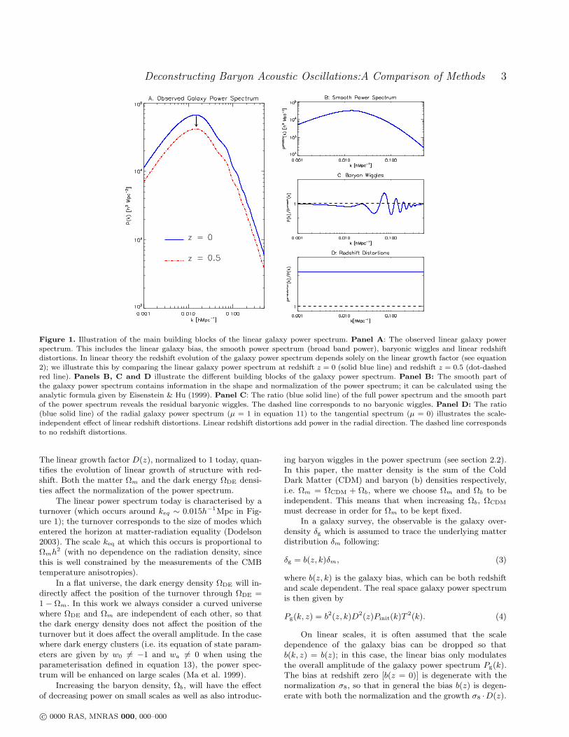
The three building blocks of the observed galaxy powerspectrum are plotted separately in Figure 1 (panels B, Cand D), while the observed power spectrum is plotted inpanel A. Each building block probes the various sectors ofthe cosmological model (dark energy, dark matter, initialconditions) in a different way. In this section, we describethe main building blocks of the power spectrum and focus ontheir cosmological parameter dependence for the following 7parameters: [Ωm,Ωb,ΩDE, w0, wa, h, ns].

2.1 Broad Band Power

The initial dark matter power spectrum is assumed to beof the form: Pinit(k) ∝ kns . The spectral index ns controlsthe tilt of the initial power spectrum, and the Harrison-Zel’dovich value of ns = 1 corresponds to a scale invariantpower spectrum of perturbations. The linear matter powerspectrum at a redshift z can be obtained by assuming theinitial power spectrum has evolved according to:

Pm(k, z) = D2(z)Pinit(k)T2(k). (2)

The quantity T (k) is the transfer function and is a solutionto Boltzman’s equations which includes the baryon wiggles.

c© 0000 RAS, MNRAS 000, 000–000

Deconstructing Baryon Acoustic Oscillations:A Comparison of Methods 3

Figure 1. Illustration of the main building blocks of the linear galaxy power spectrum. Panel A: The observed linear galaxy powerspectrum. This includes the linear galaxy bias, the smooth power spectrum (broad band power), baryonic wiggles and linear redshiftdistortions. In linear theory the redshift evolution of the galaxy power spectrum depends solely on the linear growth factor (see equation2); we illustrate this by comparing the linear galaxy power spectrum at redshift z = 0 (solid blue line) and redshift z = 0.5 (dot-dashedred line). Panels B, C and D illustrate the different building blocks of the galaxy power spectrum. Panel B: The smooth part ofthe galaxy power spectrum contains information in the shape and normalization of the power spectrum; it can be calculated using theanalytic formula given by Eisenstein & Hu (1999). Panel C: The ratio (blue solid line) of the full power spectrum and the smooth partof the power spectrum reveals the residual baryonic wiggles. The dashed line corresponds to no baryonic wiggles. Panel D: The ratio(blue solid line) of the radial galaxy power spectrum (µ = 1 in equation 11) to the tangential spectrum (µ = 0) illustrates the scale-independent effect of linear redshift distortions. Linear redshift distortions add power in the radial direction. The dashed line correspondsto no redshift distortions.

The linear growth factor D(z), normalized to 1 today, quan-tifies the evolution of linear growth of structure with red-shift. Both the matter Ωm and the dark energy ΩDE densi-ties affect the normalization of the power spectrum.

The linear power spectrum today is characterised by aturnover (which occurs around keq ∼ 0.015h−1Mpc in Fig-ure 1); the turnover corresponds to the size of modes whichentered the horizon at matter-radiation equality (Dodelson2003). The scale keq at which this occurs is proportional toΩmh2 (with no dependence on the radiation density, sincethis is well constrained by the measurements of the CMBtemperature anisotropies).

In a flat universe, the dark energy density ΩDE will in-directly affect the position of the turnover through ΩDE =1 − Ωm. In this work we always consider a curved universewhere ΩDE and Ωm are independent of each other, so thatthe dark energy density does not affect the position of theturnover but it does affect the overall amplitude. In the casewhere dark energy clusters (i.e. its equation of state param-eters are given by w0 6= −1 and wa 6= 0 when using theparameterisation defined in equation 13), the power spec-trum will be enhanced on large scales (Ma et al. 1999).

Increasing the baryon density, Ωb, will have the effectof decreasing power on small scales as well as also introduc-

ing baryon wiggles in the power spectrum (see section 2.2).In this paper, the matter density is the sum of the ColdDark Matter (CDM) and baryon (b) densities respectively,i.e. Ωm = ΩCDM + Ωb, where we choose Ωm and Ωb to beindependent. This means that when increasing Ωb, ΩCDM

must decrease in order for Ωm to be kept fixed.In a galaxy survey, the observable is the galaxy over-

density δg which is assumed to trace the underlying matterdistribution δm following:

δg = b(z, k)δm, (3)

where b(z, k) is the galaxy bias, which can be both redshiftand scale dependent. The real space galaxy power spectrumis then given by

Pg(k, z) = b2(z, k)D2(z)Pinit(k)T2(k). (4)

On linear scales, it is often assumed that the scaledependence of the galaxy bias can be dropped so thatb(k, z) = b(z); in this case, the linear bias only modulatesthe overall amplitude of the galaxy power spectrum Pg(k).The bias at redshift zero [b(z = 0)] is degenerate with thenormalization σ8, so that in general the bias b(z) is degen-erate with both the normalization and the growth σ8 ·D(z).

c© 0000 RAS, MNRAS 000, 000–000

4 Rassat et al.

2.2 Baryon Acoustic Oscillations

The baryon acoustic oscillations in the CDM power spec-trum are relatively weak features (see Figure 1); never-theless they can be used independently to constrain cos-mology (Peacock et al. 2006; Albrecht et al. 2006). Theycan be isolated from the galaxy power spectrum either bytaking the ratio with the corresponding baryon-free powerspectrum, or a smooth fitting curve (Blake & Glazebrook2003; Seo & Eisenstein 2003). In the latter case, the oscil-lations can be approximated by a decaying sinusoidal func-tion. The amplitude of the oscillations increases with thebaryon density Ωb, and the location kA of the peaks is re-lated to the sound horizon at decoupling, s, by kA = 2π/s(Blake & Glazebrook 2003).

The theoretical value of kA provides a known - or stan-dard - ruler, fixed by the sound horizon at decoupling:

s =

∫ tdec

0

csadt =

c

H0

∫ ∞

zdec

csE(z)

dz, (5)

where cs is the sound speed and:

E(z) = H(z)/H0 =√

Ωrad(1 + z)4 + Ωm(1 + z)3 +ΩDEf(z), (6)

where the expression

f(z) = exp

[

3

∫ z

0

1 +w(z′)

1 + z′dz′

]

, (7)

describes the effect of dark energy on the Universe’s expan-sion. At these high redshifts the curvature can be neglected.The radiation density is strongly constrained by the mea-surement of the CMB temperature, and the sound horizons depends strongly on Ωm through equation 6. In addition,the sound speed and the redshift of decoupling zdec dependon Ωbh

2, which is thereby moderately constrained, but apartfrom this combination, the constraints on Ωb and H0 sepa-

rately are weak due to degeneracies (though including theamplitude of the baryon wiggles would further constrain Ωb).

Dependence on dark energy parameters can vary withthe model, but in most cases the dark energy density atvery early times is small and can be neglected (Bean et al.(2001) showed it has to be less than a few percent duringthe Big Bang Nucleosynthesis epoch). The dependence onthe dark energy parameters does therefore not enter throughthe size of the ruler, it affects the observed oscillation scale:A ruler at a redshift z with a given (comoving) size r⊥(z)perpendicular to the line of sight, and a size r‖(z) along theline of sight is related to the observed angular size ∆θ andredshift extent ∆z through (Seo & Eisenstein 2003):

r⊥(z) = (1 + z)DA(z)∆θ, (8)

r‖(z) =c∆z

H(z), (9)

where DA(z) is the angular diameter distance. Since thesize of the ruler scales with s, the observation of the baryonacoustic scale in the tangential and radial direction affordsus a measurement of DA/s and H ·s respectively. In the limitwhere the size of the sound horizon is known from CMBdata to much higher precision than the measurement of theoscillation scales from the galaxy survey, we can consider the

baryon wiggles to provide estimates of the angular diameterdistance and the expansion rate directly.

Thus, if we divide out the broad shape of the powerspectrum and neglect the amplitude of the wiggles, we ex-pect to be able to measure the matter and dark energy den-sities Ωm and ΩDE; with sufficient amount of redshift infor-mation, it will also be possible to constrain the evolution ofthe dark energy equation of state w(z).

2.3 Redshift Space Distortion

An observer can only measure the galaxy power spectrumin redshift space, which is distorted compared to the powerspectrum in real space. Redshift distortions are due to pe-culiar velocities of galaxies; these cause radial distortionsin the observed galaxy density field. This distortion occursbecause the observed redshift zobs is a sum of two quantities:

zobs = zh + z~v.~r, (10)

where zh is the redshift due to the cosmological Hubble ex-pansion of the Universe, and z~v.~r is the redshift due to theradial component of the galaxy’s peculiar velocity.

In linear theory this will affect structures along the lineof sight, which will appear enhanced compared to transversestructures; i.e. for a structure which is isotropic in real space,an observer will measure more power in the radial directionthan in the transverse direction. Considering linear theoryalone, the observed redshift space power spectrum for galax-ies is related to the real space matter power spectrum by(Kaiser 1987; Seo & Eisenstein 2003):

P g,z(k, z, µ) ∝(

1 + βµ2)2

b(z, k)2Pm,real(k, z), (11)

where µ is the cosine of the angle between the wavevector ~kand the line of sight. The amplitude of the redshift distortionis modulated by the distortion parameter

β =1

b(z)

dlnD(a)

dlna, (12)

so that the redshift distortions are a probe of the growthrate of structure as well as the linear galaxy bias.

3 RECIPES FOR BARYON ACOUSTICOSCILLATIONS

The goal of this paper is to contrast the constraining poten-tial of three different families of BAO methods, namely:

(i) Full Fourier space galaxy correlation function P (k),(ii) Fourier space BAO ‘wiggles only’,(iii) Spherical harmonic space galaxy correlation function

C(ℓ).

The general underlying basis of each method is de-scribed in this section and a schematic summary is givenin Table 1. Details of the tomographic method, the fiducialcosmological model and further implementation specifica-tions are given in section 4. Full mathematical details onthe Fisher matrix calculations for each family of methodsare given in Appendix A.

c© 0000 RAS, MNRAS 000, 000–000

Deconstructing Baryon Acoustic Oscillations:A Comparison of Methods 5

Table 1. Schematic summary of which building blocks of the galaxy power spectrum are probed by each family of BAO methodconsidered in this paper. In this paper, certain components such as the normalization of the power spectrum or the redshift distortionshave been marginalized over in order to follow prescriptions which exist in the literature; when this is done the corresponding buildingblock is represented in brackets in the Table below.

Broad Band Overall Amplitude Tangential Radial Wiggle Amplitude Redshift SpacePower BAO scale BAO scale Distortions

Full P (k)√

(√)

√ √ √(√)

‘Wiggles only’ – –√ √

– –C(ℓ)

√(√)

√–

√ √

3.1 Full P(k)

The full Fourier space galaxy correlation method uses in-formation across different scales and capitalizes on eachbuilding block of the galaxy power spectrum. Such meth-ods have already been applied to forecasts for future surveys(Seo & Eisenstein 2003; Amendola et al. 2005, see AppendixA1).

In this paper we follow the implementation ofSeo & Eisenstein (2003), which we refer the reader to forspecific methodology, though details are also given in sec-tion 4 and Appendix A1.

Intuitively, because this method uses information fromthe full galaxy correlation function, it should have the po-tential to constrain cosmological parameters with high pre-cision. However since it uses information over a wide rangeof scales this method could also be prone to a high level ofsystematics.

In particular, the unknown linear bias b(z) will affectboth the overall amplitude of the power spectrum as well asthe amplitude of the redshift distortion (see equation 11). Ifthe bias is also scale dependent, i.e. if b(z) = b(k, z), thenthis can potentially distort the shape of the power spectrumover a range of scales leading to a fairly high sensitivity tosystematics.

The full galaxy correlation function will also be moresensitive to non-linear redshift distortions at small scales.Additionally, intrinsic non-linearities in the density contrastwill distort the shape of the spectrum at large wavenum-bers - while leaving the wiggle location relatively unchanged(see for e.g. Scoccimarro (2004) and Matarrese & Pietroni(2008)).

3.2 BAO wiggles only

To avoid the effect of the potential systematics of the fullP (k) method, one can focus the analysis on specific scales,and remove the overall shape and amplitude of the galaxypower spectrum, centering the analysis on the baryon wig-gles only.

The way to do this is to consider the ratio of theobserved power spectrum to a baryon-free power spec-trum, i.e. P (k,Ωb 6= 0)/P (k,Ωb = 0) (as in Figure1) or to a smooth parametric curve (Blake et al. 2006;Seo & Eisenstein 2007). This BAO ‘wiggle-only’ method hasbeen implemented in several papers. Some popular methods,

are described in Parkinson et al. (2007), Blake et al. (2006)and Seo & Eisenstein (2007).

By focusing on the baryon wiggles only, the measuredquantity is now independent of the redshift dependent lin-ear bias b(z) (though the errors on the peak measurementwill depend weakly on the bias) and, because the wiggles oc-cur on a limited wavenumber range, the measured quantityis also weakly dependent on the scale dependent bias b(k).This method should intuitively be more robust than the fullP (k) approach, as it exploits less features over a limited krange, it is also bound to provide weaker constraints on thecosmological parameters.

In this paper, the main calculations for the ‘wig-gles only’ method are performed using the formalism ofSeo & Eisenstein (2007) and Parkinson et al. (2007) (seesection 4 and Appendix A2), except in section 5.1 wherethe errors on the wiggles estimation are calculated as inBlake et al. (2006).

3.3 Spherical Harmonics C(ℓ)

Both methods described above perform the analysis inFourier space. Doing this raises several issues.

The first is that equation (11) which relates the realand redshift space Fourier power spectra is only valid inthe far field approximation, i.e. for galaxies which are sep-arated by small angles on the sky, and for which the lineof sight vectors can be considered parallel. While this maybe a valid approximation for current surveys, future sur-veys plan to cover all the extragalactic sky (∼ 2π) andthis may no longer be valid. A natural decomposition fordata on a sphere is in spherical harmonic space in whichtransverse and radial modes are independent. In this de-composition, there exists an exact solution to express thegalaxy power spectrum in redshift space (see Fisher et al.1994; Heavens & Taylor 1995, and equations A16 and A19in Appendix A). For large sky coverage it is therefore morejudicious to study the galaxy power spectrum in sphericalharmonic space.

The second and more fundamental issue has to do withthe actual measurement of the Fourier power spectrum. Thebare observables provided by a redshift survey are the angu-lar position and redshift of a galaxy, say (θ, φ, z) (althoughtechnically the redshift is itself a first order quantity derivedfrom the galaxy’s observed electromagnetic spectrum). Tomeasure the Fourier space power spectrum it is necessary

c© 0000 RAS, MNRAS 000, 000–000

6 Rassat et al.

to relate these observables to the wavenumber ~k and thistransformation is dependent on the assumed cosmologicalmodel. On the other hand, in spherical harmonic space, thetransform from (θ, φ, z) to (ℓ, z) is independent of cosmologyand this is a further central motivation for analysing galaxysurveys in spherical harmonic space.

This is the final family of methods we investigate, fol-lowing the tomographic method described in Dolney et al.(2006) (see section 4 and Appendix A3 for details).

4 IMPLEMENTATION DETAILS

In this section we describe the implementation details of ourcalculations. In section 4.1, we justify our choice of fiducialcosmological parameters and their central values. In section4.2 we describe the two fiducial surveys we use for our cal-culations, which are chosen as Stage III and Stage IV BAOsurveys as described in the DETF report (Albrecht et al.2006); these correspond to future ground and space basedsurveys respectively. In section 4.3, we overview the specifi-cations of our calculations.

4.1 Fiducial cosmological model and centralvalues

To quantify the dark energy, we adopt a convenient param-eterisation (Chevallier & Polarski 2001; Linder 2003) of itsequation of state w(a) by,

w(a) = w0 + (1− a)wa, (13)

where a = 1/(1 + z). This can also be expressed in terms ofthe pivot scale factor ap:

w(a) = wp + (ap − a)wa. (14)

The DETF “Figure of Merit” (FoM) is defined by:

FoM =1

σ(wp)σ(wa), (15)

which is used to compare the suitability of different probesand surveys to constrain the dark energy equation of state.In order to avoid problems of phantom crossing around w0 =−1, we chose a central value of w0 = −0.95.

We forecast errors for an 7-parameter model within theframework of general relativity, i.e. we have not added anyextra parameters to account for potential modified gravityscenarios (Amendola et al. 2008; Huterer & Linder 2007).The 7-parameter model and central fiducial values are givenin Table 2. The power spectrum normalization is chosen asσ8 = 0.80 and is marginalised over for calculations involvingthe full Fourier power spectrum and the spherical harmonicgalaxy correlation function.

4.2 Fiducial Survey

The DETF have published dark energy forecasts for differ-ent “Stages” of surveys, numbered from I to IV. Stage Icorresponds to dark energy projects that have already been

Table 2. Central fiducial values and cosmological parameter setfor the Fisher matrix calculations performed in section 5. Thenormalization of the power spectrum is taken as σ8=0.80 .

Parameter Central fiducial value

Ωm 0.25Ωb 0.0445ΩDE 0.75

w0 -0.95wa 0h 0.70ns 1

Figure 2. The value of kmax as a function of redshift z. Thesolid line (diamonds) corresponds σ(R) < 0.20 and kmax <

0.25hMpc−1. The dashed and dot-dashed lines correspond respec-tively to deviations around the central line, specifically kmax(z) ·0.5 (dot-dashed) and kmax(z) · 1.2 (dashed) respectively and areused in section 5.3.

completed; Stage II to ongoing projects, Stage III to “near-term, medium-cost, currently proposed projects” and StageIV to future ground or space based (LSST/SKA or JDEMlike) missions with large sky coverage. The BAO forecastspublished by the DETF were calculated using a specific im-plementation of the ‘wiggles only’ method. In this paper weare interested in comparing these forecasts with those fromtwo other methods, namely the full Fourier power spectrumand the spherical harmonic power spectrum.

We make these comparisons for future ground and spacebased spectroscopic (“S” identifier in DETF denomination)surveys, which correspond to “Stage III” and “Stages IV”surveys. In the DETF report, the spectroscopic Stage IIIsurvey is composed of both a wide and a deep survey(BAO-IIIS-o in DETF denomination, defined page 56 inAlbrecht et al. (2006)), for which results are always pre-sented combined. Here we consider only the wide survey of

c© 0000 RAS, MNRAS 000, 000–000

Deconstructing Baryon Acoustic Oscillations:A Comparison of Methods 7

Table 3. Future fiducial spectroscopic ground and space based surveys taken from DETF. The sky coverage, redshift range and galaxydensity (nP = 3) are described in the DETF report. The number of redshift bins, the bias prescription and wavenumber range are chosenspecifically for this paper.

Ground Based Survey Space Based Survey

DETF denomination BAO-IIIS-o (WFMOS-like, “wide” only) BAO-IVS-o (Optical/NIR JDEM Spatial Mission)Sky coverage 2, 000deg2 (fsky = 0.05) 10, 000deg2(fsky = 0.25)Redshift range 0.5 < z < 1.3 (4 bins) 0.5 < z < 2 (8 bins)

Bias prescription bg(z) =√1 + z

k-range kmin = 10−3, kmax < 0.25 or σ(R) < 0.20

the Stage III. For the Stage IV mission, we chose it to resem-ble a spectroscopic JDEM-like mission, by using the DETFnotation BAO-IVS-o (defined page 56 in Albrecht et al.(2006) - the optimistic survey does not include systemat-ics).

The main features of these two spectroscopic surveysare given in Table 3. The galaxy number density was takenso that neffPg(k

∗ = 0.2hMpc−1) = 3 (Blake et al. 2006;Albrecht et al. 2006), which fixes the galaxy distribution andshot noise contribution. We note that fixing the value ofneffP (k∗) does not construct a realistic magnitude-limitedgalaxy distribution. The sky coverage and redshift rangesare chosen according to the description given in the DETFreport and given in Table 3. Specifications given in the sec-ond half of the Table are chosen specifically for this paperand are explained in more detail below.

4.3 Specifications

For the ‘wiggles only’ calculation (which is the calculationperformed by the DETF) the value of the galaxy bias is ir-relevant - so long as it is scale independent, which is what weassume here. For the Fourier space and spherical harmonicspace calculations, we chose the bias to follow a simple adhoc functional form of b(z) =

√1 + z. This choice can po-

tentially affect statistical constraints for the full P (k) andC(ℓ) methods, where the bias is explicitly present; whereasthe ‘wiggles only’ method depends very weakly on the valueof the galaxy bias.

As the linear bias and normalization σ8 are highly de-generate, we also marginalise over the bias value b(zi) ineach redshift bin as well as over σ8 for the C(ℓ) method(which is slightly different than the Dolney et al. (2006) im-plementation, who uses a more complex bias prescription).

For the full P (k) method we follow the implementationof Seo & Eisenstein (2003): information from the amplitudeof the power spectrum as well as from redshift distortions aresuppressed by marginalizing over the product σ8b(zi)D(zi)and the redshift distortion parameter β(zi) in each redshiftbin. Finally, we marginalize over an unknown white shotnoise, which is denoted in Seo & Eisenstein (2003) by Pshot.

For all methods we perform calculations in the linearregime. This is ensured by restricting the calculation to cer-tain linear scales. The kmax at which non-linear effects be-come no longer negligible in our fiducial model depends of

course on the precision one wishes to attain. Recent work(Crocce & Scoccimarro 2008; Matarrese & Pietroni 2008)show that at k = 0.2hMpc−1 the deviation from linearity atz=0 is already sizeable, although the position of the peaksis much less sensitive to non-linear corrections.

The wavenumber corresponding to the linear cut-off willevolve with redshift. We quantify this evolution by con-sidering only scales for which σ(R) < 0.20 and kmax <0.25hMpc−1, where σ(R) is defined similarly to the nor-malization σ8 ≡ σ(R = 8h−1Mpc), but for a general R.The evolution of the kmax we use for our computation withredshift bin is illustrated in Figure 2 as the solid line withdiamonds. We assume the largest scales probed are given bykmin = 10−3hMpc−1.

We find the choice of wavenumber range can have a verystrong influence on results. We investigate the dependenceof the FoM on the values of kmax in section 5.3.

5 FORECASTS

The ‘wiggles only’ BAO method we use is comparable tothat used by the Dark Energy Task Force (Albrecht et al.2006, DETF), and so we first compare constraints from ourcalculation with those of DETFast2 in section 5.1. In sec-tion 5.2, we compare the constraining potential of the threedifferent families of BAO methods. The constraints are cal-culated for the galaxy surveys described in section 4, namelya future ground- and space-based spectroscopic surveys.

5.1 Comparison with DETF Calculation

In this paper, constraints for the BAO ‘wiggles only’method are performed using distance error estimates fromSeo & Eisenstein (2007). The DETF uses a similar method,though the distance error estimates are calculated us-ing the fitting formulae given by Blake et al. (2006). Theslight difference between the fitting formulae provided inBlake et al. (2006) is that the k-range is fixed, whereas inSeo & Eisenstein (2007) the k-range is an input to the er-ror estimates. In this section we switch to using the er-ror estimates from Blake et al. (2006) in order to compare

2 http://www.physics.ucdavis.edu/DETFast/ by Jason Dick andLloyd Knox.

c© 0000 RAS, MNRAS 000, 000–000

8 Rassat et al.

constraints with those given by the DETF. We obtain con-straints from DETFast1, a web-interface for calculations per-formed by the DETF.

In this calculation the central fiducial model and cosmo-logical parameter set was changed slightly to adopt the sameas that in the DETF report, i.e. ΩDE = 0.7222, Ωk = 0,w0 = −1, wa = 0, and Ωmh2 = 0.146 and the sound horizonis kept fixed. The fiducial survey was chosen to be BAO-IVS-o, as described in Table 3. Comparison between constraintsis given in Table 5; the reported constraints are shown with-out any priors (i.e. without Planck priors). Both calculationsshow agreement at the sub-percent level for all marginalisederrors (as well as for fixed errors - not shown in this table).

5.2 Comparison of different BAO Methods

For the comparison between the three different BAO meth-ods, we switch back to the fiducial cosmological modelgiven in Table 2. We also use error estimates fromSeo & Eisenstein (2007) for the ‘wiggles only’ method, inorder to have control over the k-range.

The three methods are: the full power spectrum inFourier space [P (k)], the Fourier space wiggles only method[BAO ‘wiggles only’] and the full projected power spectrumin spherical harmonic space [C(ℓ)]. In Table 4 we present themarginalised cosmological constraints for the 7-parametermodel we consider from these three different BAO methods.These constraints are marginalised over the linear bias andpower spectrum normalization (σ8) for the C(ℓ) method;for the full P (k) method we marginalise over the amplitudeof the power spectrum and the redshift distortions term asdetailed in section 4.3.

The results in brackets have been combined with fore-casted constraints from the Planck CMB mission, or whatwe refer to from now on as Planck priors. The forecastedCMB priors include scalar temperature and E-mode polar-ization information. Details on how we calculated the Planckpriors are given in Appendix B.

Parameters for which the table entry shows ‘−’, are notconstrained by the corresponding method (i.e. the affectedparameter is omitted from the Fisher matrix calculation),and we have not quantified constraints which were weakerthan 10. The cosmological constraints for different methodsare presented in Figure 3 for the dark energy parameters w0

and wa for the ground (top panel) and space (lower panel),without Planck priors.

We first explore the results from Table 4 without Planckpriors as this gives us an understanding of what each BAOmethod constrains.

We begin by exploring the ground-based survey with-out Planck priors. The ‘wiggles only’ method, which uses noinformation from the broad band power, the redshift spacedistortions nor the wiggle amplitude (see Table 1), gives con-straints which are up to a factor of 7 weaker than the C(ℓ)method. Furthermore, the ‘wiggles only’ method fails to con-strain either Ωb, wa, h and ns, whereas the C(ℓ) method onlyfails to constrain wa. The constraints from the C(ℓ) methodare a factor 2 to 18 weaker than those from the P (k) method,which can constrain wa (though the errors are still large). In

all cases, the Figure of Merits (FoMs) are small, making anycomparison between them meaningless (for very low FoMs,upper limits only are shown in Table 4).

Adding the Planck priors to the ground-based case im-proves constraints (hereafter we omit improvements on pre-viously unconstrained parameters) from the ‘wiggles only’method by a factor of 3−13, from the C(ℓ) method by a fac-tor of 1.5−10 (omitting the improvement by a factor of 300on ns), from the P (k) method by a factor of 2− 37. Includ-ing the Planck priors also reduces the differences betweenthe ‘wiggles only’ and the C(ℓ) methods (the marginalisedconstraints are of the same order of magnitude for all pa-rameters), but the constraints from the P (k) method are forsome parameters up to a factor 16 tighter than for the C(ℓ)method. The FoM for the P (k) method is over a factor of17 larger than the FoM for both the ‘wiggles only’ and C(ℓ)method.

We now consider constraints for the space-based survey,beginning with the constraints without priors.

For the space-based survey, constraints from the ‘wig-gles only’ method are a factor of 1.5−5 weaker than those forthe C(ℓ) method, and Ωb and h still remain unconstrainedfor the ‘wiggles only’ method (which is expected, since thismethod constrains only the product Ωmh2, see 2.2).

The constraints from the P (k) method remain consid-erably stronger, giving an improvement of 2 − 21 on boththe ‘wiggles only’ and the C(ℓ) method, where the largestimprovement (factor of improvement greater than 15) is onh, ns, Ωm and w0. The FoM for the P (k) method is 52, i.e.,35 times larger than that for the ‘wiggles only’ method and12 times larger than that for the C(ℓ) method.

Adding the Planck priors to the space-based case im-proves constraints from the ‘wiggles only’ method by a factorof 3 − 5, on the C(ℓ) method by a factor of 1.5 − 7 (omit-ting the factor of 40 improvement on ns), and on the P (k)method by a factor of 1.3 − 14. As with the ground-basedsurvey, the space-based survey with the Planck prior showslittle variation between the ‘wiggles only’ and the C(ℓ) meth-ods, with the Figure of Merit for each method being the sameorder of magnitude. The FoM for the P (k) with Planck pri-ors is 502, approximately 18 times larger than the FoM forthe ‘wiggles only’ method with Planck priors, and a factorof 30 tighter than C(ℓ)’ method with Planck priors.

The constraints for w0, wa, ΩDE and wp for the space-based survey, using the ‘wiggles only’ method with Planckpriors are of the same order of magnitude of those pre-sented by the DETF for BAO-IVS-o + Planck (page 77 ofAlbrecht et al. (2006)), though comparison should be takenwith caution as both use different calculations for the Planckprior as well as different methods of calculating the errorsfor the BAO calculation. The DETF report does not quoteconstraints on the other parameters, though they have alsobeen marginalised over.

In order to investigate which building block of thepower spectrum provides the most information to the P (k)method, we evaluate new constraints, this time for a quasibaryon-free spectrum (to do this we set Ωb = 0.005 as lowervalues causes numerical problems as other authors have alsofound). This test suppresses the baryon wiggles, leaving the

c© 0000 RAS, MNRAS 000, 000–000

Deconstructing Baryon Acoustic Oscillations:A Comparison of Methods 9

Table 4. Marginalised 1σ constraints from the three different BAO Methods for DETF like ground-based survey (BAO-IIIS-o) andspace-based survey (BAO-IVS-o).

Fourier space BAO ‘wiggles only’ Spherical Harmonic Space C(ℓ) Fourier space Full P (k)

Ground Based Survey (with Planck priors)

Ωm 2.04 (0.170) 0.303 (0.162) 0.137 (0.01)Ωb > 10 (0.0303) 0.122 (0.0290) 0.0310 (0.002)ΩDE 1.99 (0.156) 1.25 (0.163) 0.215 (0.016)w0 6.28 (2.42) 3.23 (1.69) 0.56 (0.25)wp 1.15 (0.184) 0.979 (0.650) 0.358 (0.07)wa > 10 (5.41) > 10 (4.45) 3.07 (0.65)h > 10 (0.238) 2.38 (0.227) 0.13 (0.016)ns - (0.00465) 1.54 (0.00465) 0.165 (0.0045)

Dark energy FoM < 0.090 (1.2) < 0.10 (0.35) 0.91 (21)

Space Based Survey (with Planck priors)

Ωm 0.181 (0.0385) 0.0367 (0.0254) 0.00985 (0.003)Ωb > 10 (0.00687) 0.0193 (0.00463) 0.00221 (0.0006)ΩDE 0.178 (0.0375) 0.113 (0.0251) 0.0692 (0.005)w0 0.990 (0.377) 0.355 (0.331) 0.0638 (0.049)wp 0.197 (0.0410) 0.147 (0.0955) 0.0313 (0.02)wa 3.94 (0.878) 1.63 (0.610) 0.612 (0.10)h > 10 (0.0539) 0.244 (0.0360) 0.0118 (0.004)ns - (0.00463) 0.182 (0.00450) 0.0106 (0.0034)

Dark energy FoM 1.5 (28) 4.2 (17) 52 (502)

Table 5. Comparison of 1σ marginalised constraints from BAO‘wiggles only’ (without Planck priors with the DETFast results.The results agree at the sub-percent level.

BAO ‘wiggles only’ DETFast

Ωmh2 0.0261 0.0258ΩDE 0.0971 0.0967Ωk 0.0308 0.0307w0 0.612 0.610wp 0.120 0.119wa 2.51 2.49

Dark energy FoM 3.32 3.37

broad band power as the only building block which nowprovides information, since the amplitude and the redshiftdistortions are marginalised over.

For the space-based survey, we find a new FoM of 11(123) without (with) Planck priors, compared to the pre-vious values of 52 (502) for the calculation including thebaryon wiggles. Though the values of the FoM for the P (k)method have dropped by about a factor of 4 when omittinginformation from the baryon wiggles, these constraints arestill an order of magnitude tighter than those for the ‘wigglesonly’ method, suggesting that a large part of the constrain-ing power of the P (k) method comes from the informationcontained in the broad band power.

Figure 3.Marginalised 1σ constraints (without Planck priors) ondark energy equation of state parameters w0 and wa for the threedifferent BAO methods: Red (dotted): Full P(k), Blue (solid):C(l), Green (hashed: BAO ‘wiggles only’. TOP: ground basedsurvey (BAO-IIIS-o). BOTTOM: space-based survey (BAO-IVS-o).

c© 0000 RAS, MNRAS 000, 000–000

10 Rassat et al.

Figure 4. Figure of Merit (FoM) as a function of normalized kmax

for the full power spectrum P (k) [dotted, diamonds], the sphericalharmonic C(ℓ) [solid, squares] and the ‘wiggles only’ [dot-dashed,triangles] methods - for the space based survey BAO-IVS-o. Thenormalized values of kmax are taken from Figure 2. The left-handpanel corresponds to constraints from the BAO methods withoutany priors, the right-hand panel includes CMB constraints fromPlanck.

5.3 Dependence of Figure of Merit onwavenumber range

We find the FoM can depend strongly on the choice of non-linear cut-off or k-range. We investigate this dependence byconsidering three different maximum wavenumbers (keepingkmin fixed at 10−3hMpc−1), namely kmax(z)·0.5, kmax(z)·1.2and the previous value of kmax(z). These three wavenumberranges evolve with redshift and have been plotted in Figure2.

The evolution of the FoM is shown for the three meth-ods considered (full P (k), spherical harmonics C(ℓ) and the‘wiggles only’) for the space-based survey (BAO-IVS-o) inFigures 4 and 5. The left hand panels in both show the re-sults without any priors and the right hand panels includePlanck priors. The FoM for the P (k) method evolves rapidlywith kmax, jumping from 3.2 at kmax(z) ·0.5 to 51 at kfid

max(z)and 80 at kmax(z) · 1.2. The evolution of the C(ℓ) method issmoother: from 0.4 at kmax(z) · 0.5, to 4.2 at kfid

max(z), and7.1 at kmax(z) · 1.2. Finally for the ‘wiggles only’ method,the evolution is slowest: from 0.2 at kmax(z) · 0.5, to 1.7 atkfidmax(z) and 2.4 at kmax(z) · 1.2. In Figure 5, we normalize

the FoM to its value at kmax(z) · 0.5 in order to quantifythe factor of improvement of the FoM as a function of kmax.This is plotted in Figure 5, with the left panel corresponding

to results without any priors, and the right panel to resultsincluding the Planck CMB priors.

Using the normalized values, we clearly see the rela-tive trends for each BAO method as a function of kmax(z).Whether we consider the results with no prior or those in-cluding the Planck CMB priors, both the P (k) and C(ℓ)methods evolve more rapidly than the ‘wiggles only’ method,and the difference is especially noticeable as we includelarger values of kmax.

The full power spectrum P (k) method contains infor-mation about the broad band power spectrum, and theamount of information used from the broad band power willdepend on the maximum wavenumber included in the Fishermatrix calculation.

6 DISCUSSION

The BAO features of the galaxy power spectrum P (k)have recently been observed in the latest galaxy surveys(Eisenstein et al. 2005; Hutsi 2006a; Percival et al. 07 a,b).They are also predicted to become a fundamental toolfor precision cosmology in the future (Peacock et al. 2006;Albrecht et al. 2006). However, there exists a range of BAOimplementations in the literature. In this paper we discussthe relative information provided by the different methods,and quantify the potential of each method to constrain darkenergy parameters.

The three BAO methods we focus on are:

• Full Fourier space galaxy correlation function P (k) (seeSeo & Eisenstein (2003)),

• Fourier space BAO ‘wiggles only’ (see Seo & Eisenstein(2007); Blake et al. (2006)),

• Spherical harmonic space galaxy correlation functionC(ℓ) (see Dolney et al. (2006)).

We do not consider the real space [ξ(r)] or configurationspace [w(θ)], correlation functions where, although the BAOsignal is larger, the non-linear and linear scales are moredifficult to separate.

Each method probes a different combination of featuresin the galaxy distribution and these are summarised in Ta-ble 1. The full Fourier space power spectrum method probesall of these features and is thus expected to provide tighterconstraints than both the ‘wiggles only’ and C(ℓ) method.The ‘wiggles only’ method probes both the radial and tan-gential BAO scales - where the C(ℓ) method only includesinformation from the tangential scale (this is because theC(ℓ) method uses the projected 2-dimensional power spec-trum). However the C(ℓ) method includes information fromthe broad band power of the projected galaxy power spec-trum.

We use the Fisher matrix formalism to forecast con-straints for two future fiducial surveys, which we choose asStage III (ground-based) and Stage IV (space-based) sur-veys as described in (Albrecht et al. 2006, DETF). The spe-cific DETF denominations for these surveys are BAO-IIIS-o(wide survey only) and BAO-IVS-o. We compare constraintsfor a 7 parameter model which allows for spatial curvature.

c© 0000 RAS, MNRAS 000, 000–000

Deconstructing Baryon Acoustic Oscillations:A Comparison of Methods 11

The evolution with redshift of the dark energy equation ofstate w(z) is parameterised as in equation 13. Our centralfiducial model in given in Table 2. The survey and implemen-tation details are given in Table 3. The choice of non-linearcut-off is justified in section 4.3, and its redshift dependenceshown in Figure 2.

In Table 5 we compare results from DETFast3 with ourcalculations and find agreement at the sub percent level, us-ing the same fiducial parameter set and values as the DETF.

The constraints for each method are presented in Ta-ble 4, without any priors and we also combine these resultswith priors from the future CMB mission Planck (the Planckpriors for the same cosmological model).

The results in Table 4 show that there exists a hier-archy between the three different methods considered here.The P (k) method which uses information from each featurein the linear galaxy power spectrum gives the tightest con-straints for both the ground-based and space-based survey.

The ‘wiggles only’ and C(ℓ) methods use different in-formation in the galaxy power spectrum. The ‘wiggles only’method uses both the radial and tangential modes, but doesnot use information from the broad band shape of the powerspectrum, the redshift distortions, nor the amplitude of thebaryon wiggles. On the other hand, the C(ℓ) method doesnot use the radial scale of the BAO scale (this is because theC(ℓ) method consists of the projected power spectrum). Onecould use the 3-dimensional decomposition of the galaxyfield in spherical harmonic space in order to recover the ra-dial BAO information as well.

Because of this, the hierarchy between the ‘wiggles only’and the C(ℓ) method cannot be predicted. Here we findthat for the two surveys considered, the constraints for the‘wiggles only’ method are weaker than those from the C(ℓ)method, themselves are weaker than constraints from theP (k) method. For the space based survey, the Figure ofMerit (FoM, defined in equation 15) for the P (k) methodis 35 times greater than that for the ‘wiggles only’ methodand 12 times greater than for the C(ℓ) method.

We also tested how the FoM for the P (k) methodchanged when a baryon-free spectrum was used. The FoMdropped by a factor of 4, but was still an order of mag-nitude larger than the FoM for the ‘wiggles only’ method,suggesting that a large part of the constraining power ofthe P (k) method comes from information contained in thebroad band spectrum.

Adding the Planck CMB priors to those from each BAOmethod reduces differences in the hierarchy. In particular‘wiggles only’ constraints with Planck priors are the sameorder of magnitude as those for the C(ℓ) method with Planckpriors. In all cases constraints from the P (k) method aretighter (with or without CMB priors).

We find the constraints can depend strongly on the cho-sen value of the non-linear cut-off, and so quantify this de-pendence for three choices of kmax(z). The evolution of theFoM (with and without Planck priors) with kmax(z) is plot-

3 http://www.physics.ucdavis.edu/DETFast/ by Jason Dick andLloyd Knox.

Figure 5. Factor of improvement of the Figure of Merit (FoM) asa function of normalized kmax for the full power spectrum P (k)[dotted, diamonds], the spherical harmonic C(ℓ) [solid, squares]and the ‘wiggles only’ [dot-dashed, triangles] methods - for thespace based survey BAO-IVS-o. The improvement is quantifiedrelatively to the value of the FoM at kNorm

max = 0.5 · kfidmax. Thenormalized values of kmax are taken from Figure 2. The left-handpanel corresponds to constraints from the BAO methods withoutany priors, the right-hand panel includes CMB constraints fromPlanck. In the left panel (without Planck priors), it is clear thatthe FoM for the P (k) methods evolves more rapidly with kmax

than the C(ℓ) method, which in turn evolves more rapidly thanthe ‘wiggles only’ method. When Planck priors are included, theFoM from the C(ℓ) method evolves more rapidly than the othertwo methods. This may be do to different parameter degeneracies.In this case, the FoM from the P (k) method evolves more rapidlythan the that for the ‘wiggles only’ method at high kmax.

ted in Figure 4. We find that there also exists a hierarchy inthe evolution of the FoM with the non-linear cut-off kmax(z).In the case where we consider the FoM from the three differ-ent methods without external priors, we find that the FoMfor the full power spectrum P (k) method depends stronglyon kmax, jumping from 3.2 to 80 for the extreme values ofkmax. The dependence of the FoM for the spherical har-monic method C(ℓ) is weaker, from 0.4 to 7.1 over the samewavenumber range; finally, for the ‘wiggles only’ method,the dependence is the weakest: from 0.2 to 2.4 for the samewavenumber range.

This suggests indeed that the ‘wiggles only’ methodpresents a more robust analysis, in that it depends weakly onthe choice of non-linear cut-off and the wavenumber range.Both the P (k) and C(ℓ) methods depend strongly on thewavenumber range, and will also depend on the linear bias

c© 0000 RAS, MNRAS 000, 000–000

12 Rassat et al.

prescription. In any case, when discussing constraints from aBAO method, it is necessary to explicitly state the methodused, as we find the FoM can vary by up to a factor of 35between different methods.

The main conclusions of this paper are therefore:

• There is not a unique BAO method, but there exists arange of implementations.

• For the three BAO implementations considered in thispaper, we find that for a given fiducial survey and cosmologythe figure of merit can vary by up to a factor of 35 betweenmethods.

• There exists a hierarchy in the constraining power of themethods. We find the more information used by a method,the higher its statistical performance, but the higher its sen-sitivity to systematics and implementations details.

ACKNOWLEDGMENTS

ARa thanks Ofer Lahav and Filipe Abdalla for useful dis-cussions on redshift distortions as well as Sarah Bridle. JWthanks Filipe Abdalla, Eiichiro Komatsu, Antony Lewis andJiayu Tang for useful discussion regarding the Planck CMBprior calculation. MK thanks Chris Blake, David Parkinsonand the Fisher4Cast team for interesting discussions andhelp with the BAO code. The authors also thank the EU-CLID cosmology working group members for useful discus-sions.

REFERENCES

Alam U., Sahni V., 2006, PRD, 73, 084024Albrecht A., Bernstein G., Cahn R., Freedman W. L., He-witt J., Hu W., Huth J., Kamionkowski M., Kolb E. W.,Knox L., Mather J. C., Staggs S., Suntzeff N. B., 2006,ArXiv Astrophysics e-prints

Amendola L., Kunz M., Sapone D., 2008, Journal of Cos-mology and Astro-Particle Physics, 4, 13

Amendola L., Quercellini C., Giallongo E., 2005, MNRAS,357, 429

Annis J., Bridle S., Castander F. J., Evrard A. E., FosalbaP., Frieman J. A., Gaztanaga E., Jain B., Kravtsov A. V.,Lahav O., Lin H., Mohr J., Stebbins A., Walker T. P.,Wechsler R. H., Weinberg D. H., Weller J., 2005, ArXivAstrophysics e-prints

Bean R., Hansen S. H., Melchiorri A., 2001, PRD, 64,103508

Benitez N. e. a., 2008, ArXiv e-prints, 807Blake C., Glazebrook K., 2003, APJ, 594, 665Blake C., Parkinson D., Bassett B., Glazebrook K., KunzM., Nichol R. C., 2006, MNRAS, 365, 255

Caldwell R. R., Doran M., 2005, PRD, 72, 043527Chevallier M., Polarski D., 2001, International Journal ofModern Physics D, 10, 213

Cimatti A., Robberto M., Baugh C. M., Beckwith S. V. W.,et al. t., 2008, ArXiv e-prints, 804

Crocce M., Scoccimarro R., 2008, PRD, 77, 023533

Dodelson S., 2003, Modern cosmology. Modern cosmology/ Scott Dodelson. Amsterdam (Netherlands): AcademicPress. ISBN 0-12-219141-2, 2003, XIII + 440 p.

Dolney D., Jain B., Takada M., 2006, MNRAS, 366, 884Eisenstein D. J., Hu W., 1999, APJ, 511, 5Eisenstein D. J., Seo H.-j., White M. J., 2006Eisenstein D. J., Zehavi I., Hogg D. W., Scoccimarro R.,et al 2005, APJ, 633, 560

Fisher K. B., Scharf C. A., Lahav O., 1994, MNRAS, 266,219

Glazebrook K., Blake C., Couch W., Forbes D., DrinkwaterM., Jurek R., Pimbblet K., Madore B., Martin C., SmallT., Forster K., Colless M., Sharp R., Croom S., WoodsD., Pracy M., Gilbank D., Yee H., Gladders M., 2007, inMetcalfe N., Shanks T., eds, Cosmic Frontiers Vol. 379of Astronomical Society of the Pacific Conference Series,The WiggleZ Project: AAOmega and Dark Energy. pp72–+

Glazebrook K., Eisenstein D., Dey A., Nichol B., The WF-MOS Feasibility Study Dark Energy Team 2005, ArXivAstrophysics e-prints

Goobar A., Hannestad S., Mortsell E., Tu H., 2006, Journalof Cosmology and Astro-Particle Physics, 6, 19

Guo Z.-K., Zhu Z.-H., Alcaniz J. S., Zhang Y.-Z., 2006,APJ, 646, 1

Heavens A. F., Taylor A. N., 1995, mnras, 275, 483Hill G. J., Gebhardt K., Komatsu E., MacQueen P. J.,2004, in Allen R. E., Nanopoulos D. V., Pope C. N., eds,The New Cosmology: Conference on Strings and Cosmol-ogy Vol. 743 of American Institute of Physics ConferenceSeries, The Hobby-Eberly Telescope Dark Energy Exper-iment. pp 224–233

Huterer D., Linder E. V., 2007, prd, 75, 023519Hutsi G., 2006a, Aap, 449, 891Hutsi G., 2006b, AAP, 446, 43Ichikawa K., Takahashi T., 2007, ArXiv e-prints, 710Kaiser N., 1987, MNRAS, 227, 1Kosowsky A., Milosavljevic M., Jimenez R., 2002, PRD,66, 063007

Lewis A., Challinor A., Lasenby A., 2000, Astrophys. J.,538, 473

Linder E. V., 2003, Physical Review Letters, 90, 091301Loverde M., Hui L., Gaztanaga E., 2008, PRD, 77, 023512Ma C.-P., Caldwell R. R., Bode P., Wang L., 1999, apjl,521, L1

Matarrese S., Pietroni M., 2008, Modern Physics LettersA, 23, 25

Mukherjee P., Kunz M., Parkinson D., Wang Y., 2008,ArXiv e-prints, 803

Nolta M. R., Dunkley J., Hill R. S., Hinshaw G., KomatsuE., Larson D., Page L., Spergel D. N., Bennett C. L.,Gold B., Jarosik N., Odegard N., Weiland J. L., WollackE., Halpern M., Kogut A., Limon M., Meyer S. S., TuckerG. S., Wright E. L., 2008, ArXiv e-prints, 803

Padmanabhan N., Schlegel D. J., Seljak U., Makarov A.e. a., 2006, ArXiv Astrophysics e-prints

Parkinson D., Blake C., Kunz M., Bassett B. A., NicholR. C., Glazebrook K., 2007, MNRAS, 377, 185

Peacock J. A., Schneider P., Efstathiou G., Ellis J. R., Lei-

c© 0000 RAS, MNRAS 000, 000–000

Deconstructing Baryon Acoustic Oscillations:A Comparison of Methods 13

bundgut B., Lilly S. J., Mellier Y., 2006, Technical report,ESA-ESO Working Group on ”Fundamental Cosmology”

Peebles P. J. E., Yu J. T., 1970, Apj, 162, 815Percival W. J., Cole S., Eisenstein D. J., Nichol R. C.,Peacock J. A., Pope A. C., Szalay A. S., 2007 b, MNRAS,381, 1053

Percival W. J., Nichol R. C., Eisenstein D. J., WeinbergD. H., Fukugita M., Pope A. C., Schneider D. P., SzalayA. S., Vogeley M. S., Zehavi I., Bahcall N. A., BrinkmannJ., Connolly A. J., Loveday J., Meiksin A., 2007 a, APJ,657, 51

Pires N., Zhu Z.-H., Alcaniz J. S., 2006, PRD, 73, 123530Refregier A., the DUNE collaboration 2008, ArXiv e-prints,802

Schlegel D. J., Blanton M., Eisenstein D., et al. 2007,in American Astronomical Society Meeting AbstractsVol. 211 of American Astronomical Society Meeting Ab-stracts, SDSS-III: The Baryon Oscillation SpectroscopicSurvey (BOSS). pp 132.29–+

Scoccimarro R., 2004, Phys. Rev., D70, 083007Seo H.-J., Eisenstein D. J., 2003, APJ, 598, 720Seo H.-J., Eisenstein D. J., 2007, APJ, 665, 14Sunyaev R. A., Zeldovich Y. B., 1970, apss, 7, 3Tegmark M., Taylor A. N., Heavens A. F., 1997, apj, 480,22

The Planck Collaboration 2006, ArXiv Astrophysics e-prints

Wang Y., 2006, Astrophys. J., 647, 1Wang Y., 2008, JCAP, 0805, 021Wang Y., Mukherjee P., 2006, APJ, 650, 1Weller J., Lewis A. M., 2003, mnras, 346, 987Yamamoto K., Bassett B. A., Nichol R. C., Suto Y., YahataK., 2006, PRD, 74, 063525

Zaldarriaga M., Seljak U., 1997, PRD, 55, 1830Zaldarriaga M., Seljak U., 1999, PRD, 59, 123507Zaldarriaga M., Spergel D. N., Seljak U., 1997, APJ, 488,1

Zhan H., Knox L., Tyson J. A., LSST Baryon OscillationScience Collaboration 2007, in American AstronomicalSociety Meeting Abstracts Vol. 211 of American Astro-nomical Society Meeting Abstracts, Cosmology with Pho-tometric Baryon Acoustic Oscillation Measurements. pp137.06–+

Zhan H., Wang L., Pinto P., Tyson J. A., 2008, apjl, 675,L1

APPENDIX A: DETAILS ON FISHERFORECASTS

It is possible to forecast the precision with which a futureexperiment will be able to constrain cosmological parame-ters, by using the Fisher Information Matrix (for a detailedderivation of the following see Tegmark, Taylor & Heavens1997 or Dodelson 2003) . This method requires only threefundamental ingredients:

• A set of cosmological parameters ~θ for which one wants

to forecast errors and a fiducial central model. The parame-ters and fiducial values we have chosen are described in theprevious section.

• A set of nmeasurements of the data ~x = (x1, x2, ... , xn)(for e.g., the spherical harmonic galaxy-galaxy power spec-trum C(ℓ) over a range ℓ = 1 ... n), and a model for how the

data depend on cosmological parameters, i.e.: ~x = ~x(

~θ)

• An estimate of the uncertainty on the data ∆(~x), whichmay depend on the given experiment (instrument noise, shotnoise, etc...) as well on the data estimator (e.g., cosmic vari-ance).

The Fisher Information Matrix (FIM) is defined by:

Fij =

⟨

∂2L∂θi∂θj

⟩

, (A1)

where L = −lnL and L = L(~x, ~θ) is the likelihood functionor the probability distribution of the data ~x, which dependson some model parameter set ~θ.

The forecasted uncertainty on the parameter θi can beestimated directly from the FIM and obeys:

∆θi >√

(F−1)ii . (A2)

By assuming the errors on the estimator ~x are Gaussianand independent, then the Fisher matrix can be estimatedby:

Fij ≃∑

n

1

(∆xn)2∂xn

∂θi

∂xn

∂θj. (A3)

The above equation holds for a single redshift; the ex-pressions for the tomographic calculation are given belowfor each BAO method.

A1 Full Fourier space power spectrum P (k)

For the case of the full Fourier space power spec-trum P (k), the Fisher matrix can be approximated as(Tegmark, Taylor & Heavens 1997; Seo & Eisenstein 2003):

Fij =∫ ~kmax

~kmin

∂ lnP (~k)∂θi

∂ lnP (~k)∂θj

Veff(~k)d~k

2(2π)3(A4)

=∫ +1

−1

∫ kmax

kmin

∂ lnP (k,µ)∂θi

∂ lnP (k,µ)∂θj

Veff(k, µ)2πk2dkdµ

2(2π)3,(A5)

where the effective volume is given by:

Veff(k, µ) =

[

n(~r)P (k, µ)

n(~r)P (k, µ) + 1

]

, (A6)

and the matter power spectrum is calculated using theCMBFast code (Zaldarriaga & Seljak 1999).

Uncertainty is the redshift determination will leave tan-gential modes unaffected and smear radial modes. This lossof information is modelled by (Seo & Eisenstein 2003):

P (~k) = Pobs(~k)e−k2

‖σ2r , (A7)

i.e. by convolving the radial position by a Gaussian uncer-tainty.

c© 0000 RAS, MNRAS 000, 000–000

14 Rassat et al.

A2 Fourier space BAO ‘Wiggles Only’

In the case of the ‘wiggles only’ method, only the size of theradial and tangential BAO scale is used. This method omitsall information from the shape and amplitude of the powerspectrum, the redshift distortion and even the amplitude ofthe BAO wiggles.

We follow the method of Seo & Eisenstein (2007), whichwe briefly summarise here. The starting point is the expres-sion to compute the Fisher matrix from the full Fourier spacepower spectrum (equation A5). The non-linear power spec-trum used is extracted from the linear power spectrum witha damping term representing the loss of information comingfrom the non-linear evolutionary behaviour. This dampingterm is approximated by an exponential computed using theLagrangian displacement fields Eisenstein et al. (2006):

Pnl(k, µ) = Plin(k, µ) exp(−k2Σ2nl), (A8)

This non-linear damping can be decomposed into theradial and perpendicular directions by:

Pnl(k, µ) = Plin(k, µ) exp

(

−k2⊥Σ

2⊥

2−

k2‖Σ

2‖

2

)

. (A9)

A delta function baryonic peak in the correlation func-tion at the sound horizon scale, s, translates into a ‘wigglesonly’ power spectrum of the form

Pb ∝ sin(ks)

ks. (A10)

This functional form is also obtained if the power spec-trum is divided by a smooth version of it or if we only usethe baryonic part of the power spectrum transfer function(e.g., Eisenstein & Hu (1999)). However, the baryonic peakis widened due to Silk damping and non-linear effects. ThisGaussian broadening translates into an exponential decay-ing factor in Fourier space:

Pb ∝ sin(ks)

ksexp

(

−k2Σ2

2

)

, (A11)

=sin(ks)

ksexp

[

−(kΣSilk)1.4

]

exp

(

−k2Σ2nl

2

)

. (A12)

We can further refine the calculation to 2 dimensions,separating the radial and tangential location of the baryonacoustic peak in the correlation function. Using the samenotation as Blake et al. (2006) and Parkinson et al. (2007),the observables are y(z) = r(z)/s and y′(z) = r′(z)/s re-spectively, where r(z) is the comoving distance to redshiftz. Measuring the fractional errors on these two observablesis equivalent to measuring the fractional errors on H · s andDA/s.

We can now use the derivatives of the ‘wiggles only’power spectrum by these quantities (see Seo & Eisenstein(2007) for all the details) to compute the Fisher matrix(equation 26 of Seo & Eisenstein (2007)). This equation in-cludes the degradation due to redshift distortions in the fac-tor R(µ) = (1 + βµ2)2 - though does not include any infor-mation from these distortions (see Table 1).

The effect of photometric redshift errors can be included

in this formalism as an additional exponential term in theredshift distortion factor, R(µ) = (1+βµ2)2 exp(−k2µ2Σ2

z),where Σz is the uncertainty in the determination of photo-metric redshifts. We evaluate these integrals to obtain theFisher matrix for the angular diameter distance, DA/s, andthe rate of expansion, H · s.

To compute the errors on the parameters, we followParkinson et al. (2007), with some changes: Since we knowthe correlation between the errors on the vector yi =r(zi)/s, r′(zi)/s, we form a small 2x2 covariance matrixfor each redshift bin, which we invert to obtain the corre-sponding Fisher matrix, F (i). While Parkinson et al. (2007)compute the transformation to the cosmological parametersanalytically, we perform it numerically.

The above is enough to provide constraints on cosmo-logical parameters. We also use another equivalent imple-mentation which adds another step and is described here-after: We form a Gaussian likelihood L ∝ exp(−χ2/2) with

χ2 =∑

i

2∑

a,b=1

∆aF(i)ab ∆b (A13)

where i runs over the redshift bins and a, b over r/s and r′/s,and ∆ = Xdata(zi)−Xtheory(zi) is the difference between thedata and the theory. We then compute numerically the ma-trix of second derivatives of χ2 at the peak of the likelihood,via finite differencing in all parameters (where it is necessaryto divide by 2 when using χ2 rather than − lnL).

A3 Spherical Harmonic space C(ℓ)

In spherical harmonic space the estimator is the galaxy-galaxy angular 2-point function C(ℓ). The Fisher matrix isthen calculated using:

Fij ≃∑

ℓ

1

∆C2gg(ℓ)

∂Cgg(ℓ)

∂θi

∂Cgg(ℓ)

∂θj, (A14)

where

∆Cgg(ℓ) =

√

2

(2ℓ+ 1)fsky[Cgg(ℓ) +Ng] , (A15)

and Ng is the galaxy shot noise.The galaxy 2-point correlation function in spherical har-

monic space is given by:

Cgg(ℓ) =⟨

|aℓm|2⟩

= 4πb2(zi)

∫

dk∆2(k)

k|Wr

ℓ(k)|2, (A16)

where aℓm represent the spherical harmonic coefficients andthe galaxy bias is taken to be constant across the depth ofeach redshift bin. The power spectrum can be expressed as:

∆2(k) =4π

(2π)3k3P (k), (A17)

and is calculated using the publicly available code CAMB(Lewis et al. 2000).

The real space window function W rℓ (k) is given by:

W rℓ (k) =

∫

drΘ(r)jℓ(kr)D(r). (A18)

c© 0000 RAS, MNRAS 000, 000–000

Deconstructing Baryon Acoustic Oscillations:A Comparison of Methods 15

The normalized galaxy distribution is denoted by Θ(r), theterm jℓ(r) refers to the spherical Bessel function of order ℓand D(r) is the growth function.

In redshift space (see section 2.3) the 2-point correlationfunction has an extra term:

C(ℓ) = 4πb2∫

dk∆2(k)

k|Wr(k) + βWz(k)|2, (A19)

where β = dlnDdlna

is the distortion term which modulated theamplitude of the distortion and

W z(k) =1

k

∫

drdΘ(r)

drj′ℓ(kr). (A20)

The reader is referred to Fisher et al. (1994) for a derivation.Padmanabhan et al. (2006) showed that this could be

re-written:

W z(k) =

∫

drΘ(r) (Aℓjℓ(kr)− Bℓjℓ−2(kr)−Dℓjℓ+2(kr)) , (A21)

where:

Aℓ =(2ℓ2 + 2ℓ− 1)

(2ℓ+ 3)(2ℓ− 1), (A22)

Bℓ =ℓ(ℓ− 1)

(2ℓ+ 1)(2ℓ − 1), (A23)

Dℓ =(ℓ+ 1)(ℓ+ 2)

(2ℓ+ 1)(2ℓ + 3). (A24)

The total galaxy window including redshift distortionscan then be rewritten:

W r+zℓ (k) = W r(k) + βW z(k) , (A25)

= W rℓ (k) + β (AℓW

rℓ (k) +BℓW

rℓ−2(k) +DℓW

rℓ+2(k)) .(A26)

So that the 2-point function with redshift distortions:

C(ℓ) = 4πb2∫

dk∆2(k)

k|W r+z

ℓ (k)|2 . (A27)

APPENDIX B: CALCULATION OF PLANCKPRIORS

The constraints from the baryon wiggles (alone or includingthe full galaxy correlation) can be combined with constraintsfrom other probes. In this paper we exploit measurements ofthe CMB anisotropies as a complementary probe; combinedwith constraints from the galaxy survey, this will tightenconstraints on some of the cosmological parameters.

The primary constraint on cosmology from the CMBcomes from the measurement of the angular size of thesound horizon at last scattering. We will use the forthcom-ing Planck mission as benchmark for a CMB prior. In orderto forecast the ability of Planck to constrain cosmologicalparameters we will need to estimate the errors on the mea-surements of the temperature and polarization power spec-tra. We will conservatively not include any B-modes in ourforecasts and assume in our fiducial model no tensor modecontribution to the power spectra.

The Fisher matrix for CMB power spectrum is given by(Zaldarriaga & Seljak 1997; Zaldarriaga et al. 1997):

FCMBij =

∑

l

∑

X,Y

∂CX,l

∂θiCOV−1

XY

∂CY,l

∂θj, (B1)

where θi are the parameters to constrain, CX,l is the har-monic power spectrum for the temperature-temperature(X ≡ TT ), temperature-E-polarization (X ≡ TE) and theE-polarization-E-polarization (X ≡ EE) power spectrum.The covariance COV−1

XY of the errors for the various powerspectra is given by the fourth moment of the distribution,which under Gaussian assumptions is entirely given in termsof the CX,l with

COVT,T = fℓ(

CT,l +W−1T B−2

l

)2(B2)

COVE,E = fℓ(

CE,l +W−1P B−2

l

)2(B3)

COVTE,TE = fℓ

[

C2TE,l + (B4)

(

CT,l +W−1T B−2

l

) (

CE,l +W−1P B−2

l

)

]

COVT,E = fℓC2TE,l (B5)

COVT,TE = fℓCTE,l

(

CT,l +W−1T B−2

l

)

(B6)

COVE,TE = fℓCTE,l

(

CE,l +W−1P B−2

l

)

, (B7)

where fℓ = ℓ(2ℓ+1)fsky

and WT,P = (σT,P θfwhm)−2 is the

weight per solid angle for temperature and polarization, witha 1σ sensitivity per pixel of σT,P with a beam of θfwhm ex-tend. The beam window function is given in terms of thefull width half maximum (fwhm) beam width by Bℓ =exp

(

−ℓ(ℓ+ 1)θ2fwhm/16 ln 2)

and fsky is the sky fraction.Note that equation B1 usually includes a summation overthe Planck frequency channels. However we conservativelyassume that we will only use the 143 GHz channel as sciencechannel, with the other frequencies used for foreground re-moval, which is not treated in this paper. This channel hasa beam of θfwhm = 7.1′ and sensitivities of σT = 2.2µK/Kand σP = 4.2µK/K (The Planck Collaboration 2006). Toaccount for Galactic obstruction, we take fsky = 0.80. Notewe use as a minimum ℓ-mode, ℓmin = 30 in order to avoidproblems with polarization foregrounds and subtleties forthe modelling of the integrated Sachs-Wolfe effect, whichdepends on the specific dark energy model (Weller & Lewis2003; Caldwell & Doran 2005).

We have now all the ingredients to calculate the Fishermatrix forecast for Planck CMB observations. However, westill have to specify the most suitable parameter set for do-ing this. It is well known that one of the primary parameterswhich can be constrained by the CMB anisotropies is the an-gular size of the sound horizon (Kosowsky et al. 2002). Alsowe should keep in mind that the Fisher matrix approachis a Gaussian approximation of the true underlying likeli-hood. In this context we would like to choose parametersin which the likelihood is as similar as possible to a Gaus-sian. Since the CMB anisotropies, with the exception of theintegrated Sachs-Wolfe effect, are not able to constrain theequation of state of dark energy it is likely that if we wouldchoose (w0, wa) as parameters for the CMB Fisher matrixthis degeneracy is artificially broken by the Fisher matrixapproach. This was also recognized by the DETF and we

c© 0000 RAS, MNRAS 000, 000–000

16 Rassat et al.

hence follow their approach to calculate the CMB Fishermatrix (Albrecht et al. 2006).

We choose as fiducial parameter set ~θ =(ωm, θS , lnAS, ωb, nS , τ ), where θS is the angular sizeof the sound horizon at last scattering (Kosowsky et al.2002), lnAS is the logarithm of the primordial amplitudeof scalar perturbations and τ is the optical depth due toreionization. Note that there might be an even more suitableparameter set, which is currently explored (Mukherjee et al.2008). The optical depth in terms of the BAO analysis pre-sented here is a nuisance parameter and we marginalise overit analytically. We then calculate the Planck CMB Fishermatrix with the help of the publicly available CAMB4 code(Lewis et al. 2000). As a final step we transform the PlanckFisher matrix in the DETF parameter set to the one usedin the analysis presented in this paper. The parametershere are given by θ = (Ωm,Ωde, h, σ8,Ωb, w0, wa, nS) byusing the transformation with the Jacobian

Jαα =∂θα

∂θα(B8)

and the Fisher matrix in our set of basis parameters

F = JFJT . (B9)

This paper has been typeset from a TEX/ LATEX file preparedby the author.

4 http://camb.info

c© 0000 RAS, MNRAS 000, 000–000