1

DECENTRALIZING SEMICONDUCTOR CAPACITY PLANNING VIA INTERNAL MARKET COORDINATION

SULEYMAN KARABUK and S. DAVID WU

Manufacturing Logistics Institute, Department of Industrial and Manufacturing Systems Engineering, Lehigh University, Bethlehem, Pennsylvania, david.wu@lehigh.edu

Abstract

Semiconductor capacity planning is a cross-functional decision that requires coordination

between the marketing and manufacturing divisions. We examine main issues of a decentralized

coordination scheme in a setting observed at a major US semiconductor manufacturer: marketing

managers reserve capacity from manufacturing based on product demands, while attempting to

maximize profit; manufacturing managers allocate capacity to competing marketing managers so

as to minimize operating costs while ensuring efficient resource utilization. This cross-functional

planning problem has two important characteristics: (1) both demands and capacity are subject to

uncertainty, and (2) all decision entities own private information while being self- interested. To

study the issues of coordination we first formulate the local marketing and the manufacturing

decision problem as separate stochastic programs. We then formulate a centralized stochastic

programming model (JCA), which maximizes the firm’s overall profit. JCA establishes a

theoretical benchmark for performance, but is only achievable when all planning information is

public. If local decision entities are to keep their planning information private, we submit that the

best achievable coordination corresponds to an alternative stochastic model (DCA). We analyze

the relationship and the theoretical gap between JCA and DCA, thereby establishing the price of

decentralization. Next, we examine two mechanisms that coordinate the marketing and

manufacturing decisions to achieve DCA using different degrees of information exchange. Using

insights from the Auxiliary Problem Principle (APP), we show that under both coordination

mechanisms the divisional proposals converge to the global optimal solution of DCA. We

illustrate the theoretic insights using numerical examples as well as a real-world case.

2

1. Introduction

Production capacity is the most significant portion of capital investment in semiconductor wafer

manufacturing. Effective utilization and management of production capacity have significant

implications to the profitability of the operation. Capacity planning in the industry typically

entails strategic, and operational planning organized in a hierarchical manner. Strategic planning

decis ions specify which microelectronics technology at what capacity level within what

timeframe is in need to meet expected future demands, and which fabrication (fab) facilities

should be equipped and certified to product with which technologies (Karabuk and Wu, 1999).

Given the strategic fab configuration, operational planning specifies, in a short-term and

dynamic basis, the actual number of “wafer starts” of particular technologies at each facility. In

this paper, we will focus our attention on the operations planning aspects of capacity

management, which is known in the industry as the capacity allocation problem. Capacity

allocation typically involves multiple fab facilities of the firm, each with different manufacturing

capabilities, as well as yields, costs, lead-times, and quality expectations. Typical planning

period is one week, while the overall planning horizon covers several weeks.

Manufacturing of microelectronics products consists of silicon wafer production (known as the

“front-end” operations), followed by assembly, testing and packaging (the “back-end”

operations). Front-end operations consist of the most crucial part of the process as it has a long

manufacturing cycle time, and it represents the most significant portion of the capital

investments. The overall manufacturing cycle time is typically in the range of 20-40 days, about

15-35 of which is spent in the wafer fab. Back-end operations such as packaging, assembly and

test, are typically carried out in geographically separated facilities (many are overseas), whose

operations are typically not the bottleneck in the production cycle. This research is based on

decision problems within a global capacity planning group at a major US semiconductor

manufacturer. Our focus will be on the allocation of front-end manufacturing capacity across

multiple wafer fabs around the globe. Although there are a great variety of end products (over

2,000), they are categorized by aggregated technology families distinguished by the underlying

manufacturing processes, and the equipment requirements. All capacity allocation decisions are

based on aggregate technologies rather than end products.

3

One important characteristic of semiconductor capacity planning is the uncertainty in both

demands and capacity. Demand uncertainty is due to the volatile nature of high-tech industries

such as telecommunication, computers, and electronics. A microelectronics chip which faces

high demand today may be quickly outdated in a few months with the introduction of a next-

generation chip that requires upgraded technology. Uncertainty is even more pronounced in the

short-term. Customers may change their orders frequently and significantly; for some the

fluctuation of order quantity (of a certain future week) could average as much as 100% over the

history of the order. Worse, customers may only communicate their demand profile over a short

period into the future. Due to the long production lead-time, manufacturers must expand their

“order view” by forecasting demand beyond what their customers would provide. On the other

hand, capacity uncertainty is a fact of life in the industry due to the needs to continually upgrade

fab facilities. New manufacturing processes introduce high variability in production yields and

consequently cause uncertainty on manufacturing throughput. On the other hand, in order to

achieve economies of scale, large production batches are commonplace. This means that extreme

outcomes in a particular demand and capacity realization can lead to long- lasting business

consequences difficult to recover from. It is imperative for planners to consider uncertainties

explicitly and strategically so as to hedge operational decisions against extreme outcomes.

Another industry reality of the capacity allocation problem is that demands and capacities are

typically managed by different decision entities in the semiconductor firm. It is common

practice in the industry to delegate these capital- intensive decisions to different divisions in order

to establish proper check and balance, and to maintain accountability. This could also ease the

complexity of information gathering, processing, and decision-making. In our case, product

managers (PMs) in different SBU’s (strategic business units) manage demands, serving

marketing and customer relation functions, while manufacturing managers (MMs) at each fab

facility manage capacity, ensuring its efficient utilization. Thus, not only are demand and

capacity both exogenous sources of uncertainty, they are also endogenous factors within the firm

due to different perspectives in the management structure. Product managers represent the

marketing perspective where customer satisfaction and revenue maximization are the main goals.

Manufacturing managers represent the perspective where the efficient utilization of resources,

4

and the reduction in operating cost are the main goals. Besides the reward structure, also

important is where reside the insights and the information required for reliable decisions. Product

managers have the expertise and often the information concerning the behaviors of their

customers, who might be able to anticipate possible changes in demand. PMs also have up-to-

date information about market trends, and they could sometimes predict a softening or

strengthening market for some products. Similarly, manufacturing managers could make use of

their experience about the equipment, the yields, and the loading status of production to adjust

capacity allocation. Nonetheless, the marketing and manufacturing perspectives are often in

conflict, which need to be reconciled and coordinated in order to maximize the overall efficiency

of capacity usage. However, centralized planning process in modern ERP systems has difficulty

incorporating local information, let along accommodating local perspectives. A main reason is

that much valuable local information is privately held by managers motivated to leverage which

for local benefits. In this paper, we will explore insights required for a decentralized coordination

mechanism, which allow PMs and MMs to reconcile their local interests with global efficiency.

In the following, we first summarize main literature and previous work related to the research.

Related Literature

We will characterize uncertainty and coordination in the above decision environment using

structural insights from stochastic programming model with recourse. In the broader literature of

stochastic programming for capacity and production planning problems we point to a few

representative and relevant studies in the following. Bienstock and Shapiro (1988) model

resource acquisition decisions as a stochastic program with recourse. They apply the model at an

electric utility to make fuel contracting and plant construction decisions under demand

uncertainty. In a frequently cited study, Eppen et al. (1989) model the capacity-planning problem

of a major automobile manufacturer. Their model makes facilities configuration decisions for the

production of different automotive models, and at the same time making shut-down decisions for

some of the product lines. Demand over the medium term planning period is treated as random.

Berman et. al. (1994) propose a stochastic programming model for the capacity expansion

problem in service industry with uncertain demand. Their model decides the size, location, and

timing of the expansions so as to maximize the total expected profit. Escudero et al. (1993)

summarize different stochastic programming models for the production and capacity planning

5

problem. The decisions considered are production volume, product inventory, and resource

acquisition decisions under uncertain demand. Power generation planning is another problem

that has been modeled by various stochastic programming models (c.f., Takriti et. al. (1996)). In

all these applications, demand is the major source of uncertainty.

Porteus and Whang (1991) and Kouvelis and Lariviere (2000) also examine internal market

mechanisms for manufacturing capacity where incentive schemes are developed to induce

system-optimal actions from marketing and manufacturing. However, their coordination is

assumed at a more aggregate level where the decision maker’s decision could be described by

strictly convex, functional optimization problems. The coordination scheme is developed based

on transfer payments derived a priori from the closed-form solution of the decision problem. Our

analysis considers more detailed coordination under various demand and capacity scenarios in a

mathematical programming setting.

Coordinating divisions in a multi-divisional firm by means of mathematical decomposition has

been a subject for earlier OR research (Dantzig and Wolfe (1961), Kate (1972), Christensen and

Obel (1978), Burton and Obel (1980), Luna (1984)). The most commonly used approach is to

apply either Dantzig-Wolfe decomposition or Lagrangean relaxation to facilitate coordination.

The problem is solved iteratively by alternatively solving for the relaxed problem (i.e.

subproblems) and adjusting the prices (solve master problem as in Dantzig-Wolfe or subgradient

search as in lagrangean relaxation) until the optimal price vector is found hence the original

problem solved. The economical interpretation of this solution process is that, a coordinator

assigns prices on the common resources and decision makers solve their local problem with the

given prices and submit proposals. After the prices are adjusted to bring demand and supply

closer, the same decision making process continues in an iterative manner. However, there is a

serious shortcoming of this approach in that competitive equilibrium can not be reached at the

end of the iterations. That is, after the prices are finalized and the solution is found, the

participants have incentives to trade in an after market and actually implement a different

solution than the one found by coordination. There are a few studies that address this limitation.

Jennergren (1972) proposed a modification to Dantzig-Wolfe decomposition, which perturbs the

objective functions of the subproblems by a quadratic term. Jose et. al. (1997) provide an in-

6

depth analysis of the issue and generalize Jennergren’s work in the context of auctions. Ertogral

and Wu (1999) study a similar coordination mechanism in the context of production planning in

the supply chain. They design an auction-theoretic mechanism for multiple production facilities

using insights from Lagrangian decomposition. Kutanoglu and Wu (1999a) show that

Lagrangian relaxation, as a means of price coordination is a version of Walrasian auction

t>tonnement that lead to non-zero duality gap for non-convex optimization problems. To

eliminate the duality gap Walrasian t>tonnement could be generalized to augmented t>tonnement

using non-linear pricing.

2. The Semiconductor Capacity Allocation Problem

The semiconductor capacity allocation problem is a combination of marketing and

manufacturing problems. The product managers (PMs) and manufacturing managers (MMs) are

key decision entities representing interests of the marketing and the manufacturing divisions,

respectively. PMs are each responsible for a subset of product demands typically defined by

customers from a specific market sector (e.g., telecommunications, multimedia devices, disk

drives). Each PM must satisfy his/her customers on one hand while competing for (scarce)

production capacity on the other. Their performance evaluation is mainly based on the total

sales achieved; hence, they aim to meet all the anticipated demand throughout the planning

period. MMs are each responsible for a subset of production capacity typically defined by fab

facilities with a specific generation of production technology (defined by line-width, wafer size,

etc.). Each MM must accommodate the requests from the PMs while ensuring the efficient

utilization of his/her facility. Performance evaluation of the MMs is mainly based on operational

costs, which drives their capacity allocaiton decisions. While the PMs and MMs typically have

their own decision problems clearly defined, the collection of these decisions could be far from

maximizing overall corporate profits. It is imperative to establish coordinated marketing-

manufacturing solutions while preserving the decentralized organizational and information

structure defined by the PMs and MMs. To explore such coordination scheme, in the following,

we will further detail the decision problems faced by the PMs and MMs and develop two

stochastic decision models from their points of view. We will then introduce the notion of

coordination in this context and suggest methods that reconcile the two perspectives using

insights from Augmented Lagrangian.

7

2.1. The Marketing Problem

Let xijt denote the amount of wafer supply that the PMs require for technology i (i∈M) from

facility j (j∈F) during planning period t (t ∈T). Although we do not explicitly include lead-times

in the formulation, we interpret the planning periods as (t + lead-time). Define g(.) as the profit

function (as perceived by the PM) associated with allocation x. Without the lose of generality,

we assume the demands for a technology is Gaussian and can be captured in the form of demand

scenarios represented by set S1. Let ps be the probability associated with s∈S1. Each scenario

s∈S1 corresponds to a demand vector ds={dits, ∀ i∈M, t∈T} that covers all technologies over all

periods. Under a particular demand scenario s, it may be the case where the allocated production

capacity is not sufficient to cover the realized demand. In this case, there are two recourse

actions that could take place: make use of inventory Iits, carried from an earlier period, or

outsource capacity Oits from a contracted outside foundry with additional cost. In the cases where

outsourcing is not possible, the outsourcing costs can be interpreted as the costs of lost demands.

Backordering is usually not an option in this environment due to high demand volatility and

short product lifecycle. The basic decision problem for the PM can be stated as a two-stage

stochastic program as follows, where xijt is the first stage decision variable while Iits and Oits are

the second stage recourse variables. The demand uncertainty known to PM is characterized by

scenario set S1.

The Marketing Problem (PM)

)1()()(1}).(:{

∑∑∑∑ ∑ ∑∈ ∈∈∈ ∈ ∈

++−=Tt Mi

itsOitits

Iit

Sss

Mi Njij TtijtPM OcIcpxgz

Minimize

)2(,,

..

11 SsTtMidOIIx

ts

itsitsitssitFj

ijt ∈∈∈∀=+−+ −∈∑

The first stage objective is to maximize the PM’s utility. With cIit, cO

it denoting the unit costs

associated with the variable in the superscript, the second stage problem is to minimize the

expected inventory and outsourcing costs over the planning periods. Constraints (2) state that

8

demands must be satisfied by either first-stage capacity allocation, or by recourse actions via

inventory positioning, or outsourcing.

2.2. The Manufacturing Problem

An MM allocates capacity at the wafer fab by determining the quantity of wafers to be released

into the system to meet demands at the end of the manufacturing period. Thus, capacity

allocation is measured in terms of wafer starts. Released wafer lots typically experience cycle

time variability throughout the manufacturing period, every lot yields an uncertain amount of

microelectronic chips at the end of the process. Thus, the number of wafer starts is determined

based on the planned number of wafers at the end of the process; the actual quantity can be lower

or higher than the planned wafer output. For modeling purposes, we express this as capacity

uncertainty characterized by normally distributed random variables. The variance of the

distribution is expressed as a fraction of the expected yield and is known to the MM.

Let yijt denote the quantity of wafer starts for technology i (i∈M) at facility j (j∈F) during

planning period t (t∈T). We represent capacity uncertainty by scenarios set S2. Each scenario

s∈S2 corresponds to a yield vector ys={kijsyijt, ∀ i∈M, ∀ j∈F, t∈T} that covers all facilities,

technologies and periods. Parameter kijs is the yield coefficient associated with technology i at

facility j in scenario s. Thus, the term kijsyijt corresponds to the realized production for technology

j under scenario s given the planned quantity yijt. Note that we use the term “yield” in a broad

sense referring to the actual production quantity at the end of the manufacturing cycle. From the

viewpoint of the MMs, the PMs are customers who specify their capacity requests (in wafer

starts) as xijt. The MMs make their wafer start decisions based on this request and are liable for

the consequences should there be deviations between the actual and the requested amount.

Denote δ−, δ+ the recourse variables that measure for the yield deviations from the PM requests

with an underage and overage costs, cuit and co

it, respectively. We now state a two-stage

stochastic program for the MM’s decision problem as follows, where the capacity uncertainty

known to MM is characterized by scenario set S2.

The Manufacturing Problem (MM)

9

)'1()(

)(

2

2

∑∑∑∑

∑∑ ∑∑∑∑

∈ ∈ ∈

+−

∈

∈ ∈ ∈∈ ∈ ∈

++

−+=

Mi Fj Ttijts

oitijts

uit

Sss

Fj Ttjt

Miijtij

Ujt

Mi Fj Ttijt

yijMM

ccp

Ueyacycz

Minimize

δδ

)3(,,,0

..

2SsTtFjMiyk

ts

ijtsijtsijtijs ∈∈∈∈∀=−+ +− δδ

)4(, TtFjeya jtMi

ijtij ∈∈∀≤∑∈

)5(,, TtFjMiegya ftfmijtij ∈∈∈∀≤

The first-stage objective is to minimize the MM’s operating costs as defined by the variable

production cost, cyij, and the capacity under-utilization cost cU

jt. Let aij be the capacity

consumption rate for technology i at facility j, and ejt be the total capacity at facility j during

period t, the second term in the objective defines a quadratic penaly for violation of the capacity

utilization target. Equipment constitutes the most significant capital investment in semiconductor

manufacturing. Utilization of existing capacity either beyond or below a manufacturing target

level U is both undesirable. When facilities operate beyond a certain utilization level, throughput

may drop significantly due to increased equipment failures and congestion in the system. When

the converse is true, it would be hard to justify the return on investment. It is common in the

industry to set the target at as high as 90%. For further discussion of the utilization target, see

(Karabuk and Wu, 1999). The second stage objective is defined by the underage or overage

adjustments from the PM request under each senario s∈S2. Constraints (3) measure the

deviations of actual production quantities from the planned quantities (by δ−, δ+) under each

yield scenario. The total capacity constraints for each facility in each period are stated in (4). To

ensure operational stability, facility j may set forth restrictions that limit the maximal proportion

of capacity (gij) that could be allocated to a particular technology i. This is expressed by

constrains (5).

3. Coordinating Marketing and Manufacturing Decisions

With the marketing and manufacturing local problems defined, we will now explore the issue of

coordination. First, it should be clear that without coordination the PM and MM local decisions

10

are unlikely to achieve agreement (i.e., the capacity allocation xijt≠yijt for some i,j,t), and second,

these local decisions may be far from optimizing overall corporate profits. In the following, we

first establish a theoretical target for coordination.

3.1 The Theoretical Target of Coordination

To establish a goal for the coordination of marketing and manufacturing decisions, we envision a

joint optimization model of the PM-MM local problems with the following requirements: (1) the

demand and capacity scenarios considered by PM and MM respectively must be evaluated

jointly, (2) the objective function must be a convex function of the local problems, and (3) local

decisions from both sides must agree with each other. Note that, while formulating such a joint

model may not be meaningful with respect to the organizational and information structure of the

real problem, it is useful to consider this conceptual model as a step toward strategizing a

coordination scheme between the PMs and MMs. Consider a joint PM-MM optimization

problem as a two-stage stochastic program as follows.

Joint Capacity Allocation Problem (JCA)

)1()()(

)())((

221

2

′′++++

−+−=

∑∑ ∑ ∑∑∑∑

∑∑ ∑∑∑ ∑

∈ ∈ ∈ ∈ ∈ ∈

+−

×∈

∈ ∈ ∈∈ ∈ ∈

Tt Mi Ss Mi Fj Ttijts

oitijts

uitsits

Oitits

Iit

SSss

Fj Ttjt

Miijtij

Ujt

Mi Fj Ttijtijt

zijJCA

ccpOcIcp

Ueyacxgycz

Minimize

δδ

)3(,,,0

)2(,,

)6(,,

)5(,,

)4(,

..

2

211

SsTtFjMiyk

SSsTtMidOIIxk

TtFjMiyx

TtFjMiegya

TtFjeya

ts

ijtsijtsijtijs

itsitsitssitFj

ijtijs

ijtijt

ftfmijtij

jtMi

ijtij

∈∈∈∈∀=−+

′′×∈∈∈∀=+−+

∈∈∈∀=

∈∈∈∀≤

∈∈∀≤

+−

−∈

∈

∑

∑

δδ

The joint capacity allocation problem can be viewed as a centrally coordinated marketing and

manufacturing decision problem that combines PM’s and MM’s original problems in a stochastic

programming model with recourse. However, the recourse in this problem (defined by (1)″, and

11

(2)″, (3)) uses joint demand-capacity scenarios S1×S2 as opposed to the decomposed scenario

structure S1 and S2 in the local problems. Constraints (6) ensure that the marketing and

manufacturing decisions agree with each other.

To define a coordination mechanism that could be implemented in realistic marketing and

manufacturing interfaces, we require that the mechanism should not require decision makers to

reveal private information. More specifically, we require the coordination mechanism to solve

the capacity allocation problem in a decentralized manner using the PM and MM subproblems,

which requires decentralized decision authority and local scenario information. Within the (JCA)

model, the manufacturing subproblem can be viewed as a two stage stochastic programming

model with recourse, where x are stage 1 decisions subject to stage 1 constraints (4) and (5), and

yOI ,,,, +δδ are recourse variables subject to recourse constraints (2”), (3) and (6). The

marketing subproblem can be described in a similar fashion. Nevertheless, this decomposition of

the marketing and manufacturing problems requires the sharing of private information: the

manufacturing problem must have access to true demand scenarios, and similarly the marketing

problem must have access to true yield scenarios. Therefore, (JCA) does not satisfy the basic

requirements for a coordination mechanism, further, it may not be computationally feasible to

deal with scenario set S1×S2. To design a coordination mechanism that operates within a

decentralized marketing and manufacturing structure while achieving results approximate that of

(JCA), we define a Decentralized Capacity Allocation (DCA) problem as a straightforward

combination of the marketing and manufacturing local problems as follows:

(DCA) (6)-(2) s.t.

Minimize PMZMMZDCAZ +=

The main difference between (JCA) and (DCA) comes from the assumption on information

availability: the former assumes that a centralized decision entity have full information on both

demand and yield scenarios, and is in the position to evaluate all possible combinations of these

scenarios (i.e., S1×S2). The later assumes that full information is not available to any one entity,

and the local scenario sets S1 and S2 must be evaluated separately and independently. This is

reflected by the difference between constraint sets (2) and (2”). In fact, the recourse represented

by (2) fix the yield scenario for all demand scenarios considered, i.e., set kijs=1

21,, SSsFjMi ×∈∈∈∀ . The gap between the solutions of the (DCA) and (JCA), as

12

characterized by Propositions 1 to 4 in the following section, should be considered the price for

decentralization in decision-making.

3.2 The Relationship between DCA and JCA

JCA establishes the theoretical goal for coordination while DCA represents an achievable goal

when information privacy is required. In the following, we establish main analytical relationships

between (JCA) and (DCA).

Proposition 1: Let QJCA(x, ks, ds), QDCA(x, ks=1, ds) represent the recourse for the (JCA) and

(DCA) problems, respectively. Then the following relation holds.

QDCA(x, ks=1, ds) ≤ QJCA(x, ks, ds) ∀ x

Proof:

For any given capacity allocation vector x and demand scenario ds the function ), d, kx(Q ssJCA is

convex and piecewise linear. The linear function )d1,k ,x(Q ssDCA = bounds the other from below.

When the ks=1 takes the expected value for the yield scenarios, then the proposition follows

from the properties of the Jensen’s lower bound (Kall and Wallace 1994).�

Proposition 1 states that the recourse in model (DCA) approximates the recourse of the (JCA)

from below. Consequently, the capacity allocation solution of the (DCA) model constitutes an

upper bound for the (JCA) model. In the following, we will provide some insights on the gap

between the recourse functions QDCA(.) and QJCA(.) by characterizing dual prices of the recourse

constraints, and by the problem structure specific to capacity allocation.

Proposition 2: Define G(x) to be the gap between QDCA(.) and QJCA(.) for any given capacity allocation vector x. Then, G(x) can be expressed as follows:

21

2121

21212121))(()( )2(

)1:()"2(

ssSSss Mi Tt Fj

ijtsijssitsksitssits pxkdxGijs∑ ∑∑ ∑

×∈ ∈ ∈ ∈= −−= ππ

where π corresponds to the dual prices associated with the constraint set indicated by the superscript. Proof: For any given capacity allocation solution x , the recourse of the (JCA) model can be

expressed in terms of dual prices as follows (by duality theorem):

∑∑∑∑∑ ∑∑ ∑∈ ∈ ∈ ∈×∈ ∈ ∈ ∈

+−=2

21

2121

212121

)3()"2(ss )()d ,k,x(

Ss Mi Fj Ttsijtijsijtsss

SSss Mi Tt Fjijtsijssitssits

JCA pxkpxkdQ ππ (a)

13

Similarly, the recourse of the (DCA) model can be expressed as follows:

∑∑∑∑∑ ∑∑ ∑∈ ∈ ∈ ∈×∈ ∈ ∈ ∈

= +−==22121

212121

)3()2()1:(ss )()d 1,k,x(

Ss Mi Fj Ttsijtijsijtss

SSss Mi Tt Fjijtsijssitsksits

DCA pxkpxkdQijs

ππ (b)

This expression comes from the observation that the particular lower bound that the QDCA(.)

implements is obtained by using the joint scenario set but with a single dual basis for the yield

scenario set. Since G(x)= (a) – (b) the proposition follows. �

Proposition 3: Let ∑∈

−=∆Fj

ijtijsitsits xkdd be the demand-supply gap associated with the joint

scenario s. Consider period t’ for any technology i, and scenario s: if sit

d '∆ is nonnegative then

π it’s= cOit’. If sit

d '∆ is negative, then π it’s depends on itsd∆ (t > t’) values of succeeding periods.

Suppose t” is the first period after t’ at which sit

d "∆ is positive, then ∑=

−="

'"' )(

t

tt

Iit

Oitsit ccπ .

Proof. This proposition follows from the basic properties of dual prices. When itsd∆ is

nonnegative, there is a capacity shortage. Thus, increasing itsd∆ by 1 unit would increase the

right hand side of constraints (2)” by 1 unit, which in turn increases the shortage Oits by 1 unit. ''

211 )2(,, SSsTtMixkdOIIFj

ijtijsitsitsitssit ×∈∈∈∀−=+− ∑∈

−

This increases the objective function value zJCA by cOit, i.e., π it’s= cO

it’. Similarly when itsd∆ is

negative, there is excess inventory and decreasing the right hand side by 1 unit causes 1 unit of

extra inventory Iits to be carried until it is used to compensate for 1 unit of shortage at a future

period. If t” is the first period after t’ at which sit

d "∆ is positive, this incurs an inventory cost of

∑=

"

'

)(t

tt

Iitc , thus we have ∑∑

==

−=−−="

'""

"

'' )()(

t

tt

Iit

Oit

Oit

t

tt

Iitsit ccccπ .�

Proposition 2 relates the gap between recourses QDCA(.) and QJCA(.) to the dual prices and show

that the size of the gap depends on the differences between the dual price vectors for constraint

sets (2) and (2)", and the supply-demand gap. Proposition 3 further shows that the dual prices

are determined by the capacity shortages or overages under each joint scenario s∈S1×S2. In the

following, we state a sufficient condition where the gap can be completely closed.

14

Proposition 4: For a given stage 1 solution x , QJCA( x , ks, ds)=QDCA(x , ks=1, ds) if the following holds. Let ∑

∈

−=∆Fj

ijtsijssitssits xkdd212121

. For all 11 Ss ∈ , Mi ∈ , and all periods t

If 0)1:( 21≥∆ =ijsksitsd , then 0

21≥∆ sitsd for all 22 Ss ∈ , and

If 0)1:( 21<∆ =ijsksitsd , then 0

21<∆ sitsd for all 22 Ss ∈

Proof: By Proposition 2 the gap between (DCA) and (JCA) depends on the difference in dual

prices associated with the solution of QJCA(.) and QDCA(.). By Proposition 3, if the sign of

21 2121 and == ∆∆ sitssits dd are the same for all i and t,, then 1s 21 =sπ = 2s 21 =sπ . Therefore, if the conditions

stated in the proposition holds, then the recourse computed by (JCA) and (DCA) at point x will

be equal. �

An important implication of Proposition 4 is that at “extreme” capacity allocation solutions x ,

defined as the cases where 21sitsd∆ represents a high level of capacity shortage or excess

inventory for technology i in period t such that the sign of the gap 21sitsd∆ is the same for all

22 Ss ∈ , the (DCA) model will correctly represent the (JCA) model. On the other hand, since the

yield scenarios are summed for each technology in each period, extreme positive and negative

yield realizations may cancel each other out even if the sign of the gap does not completely agree

with each other. This later situation will also strengthen the approximation of the QDCA(.).

Another observation is that, as the unit inventory holding and outsourcing costs increase, the

differences in dual prices increases, thus the gap G(.) also increases. Similarly, as the variability

of demand scenarios and the yield scenarios increase, the magnitude of dual price differences

across yield scenarios will increase, therefore the gap G(.) will increase.

From the propositions, one could conclude that in the situations where demand and capacity

scenarios are independent, when the cost of demand-capacity mis-matching is low, or when the

variation on demand and capacity is low, the approximation gap is expected to be small. With

this established, we now describe coordination mechanisms designed to achieve the optimal

solution defined by (DCA) while satisfying the information privacy requirements. As stated

previously, the gap between JCA and DCA should be viewed as the price of coordination. From

the above propositions, one could conclude that the size of the gap is determined by the

dependency between demand and capacity scenarios, the marginal costs of demand-capacity mis-

15

matching, and the variation on demand and capacity scenarios. In the following, we will describe

coordination mechanisms designed to achieve the optimal solution defined by (DCA).

3.3. Coordination Mechanism for the Marketing and Manufacturing Problems

The coordination problem between manufacturing and marketing divisions can be interpreted as

finding a set of transfer pricing between the buyers (PMs) and the sellers (MMs) in an internal

market where manufacturing capacity is the economical commodity. In the decision making

framework we propose, the headquarter (i.e. central authority) sets generic rules regarding the

rights and obligations of the participants and endows the divisions with complete control over

how much to trade at what quantities. The negotiations (iterations) terminate when the division

managers mutually agree on a fixed price quantity transaction. This is a commonly used

approach in the accounting and applied economics literature to facilitate coordination between

divisons of a firm such as marketing and manufacturing. The transfer prices that will coordinate

the capacity allocation problem should have the property that both PMs and MMs solve their

local problems and come up with the same solution which also solves the capacity allocation

problem (DCA) optimally. Otherwise, the solution will not be supported by the local decision

makers and will likely to be altered during execution. In the following we present two

coordination mechanisms using the notion of tranfer pricing as a means to achieving

coordination that corresponds to the system optimal. Both mechanisms are motivated by

mathematical decomposition via Augmented Lagrangian.

Recall that xijt denote the amount of wafer supply that the PMs require and yijt the wafer supply

quantity offered by the MMs. We say that the coordination is consistent when wafer supply

proposals from PMs (xijt) and MMs (yijt) agree, that is xijt =yijt for all technology i, facility j and

planning period t. We say that the coordination achieves proactive equilibrium when the wafer

supply proposal is consistent and the proposal corresponds to an optimal solution to the

decentralized optimization problem (DCA). Since neither (PM) nor (MM) have closed form

solutions, we will not be able to establish the transfer pricing a priori. Instead, we propose a

coordination mechanism between (PM) and (MM) that would iteratively determine the transfer

pricing using earlier information communicated by the other side. The procedure stops when the

PM and MM solutions converge and become consistent with one another. Importantly, when a

16

proper transfer pricing is found at convergence, the coordinated solution will correspond to the

optimal of (DCA).

Finding a proper form of transfer pricing is a nontrivial task. Jennergren (1972) proposes a

quadratic perturbation scheme for the subproblem objectives, which can be viewed as a

randomized search of the optimal transfer pricing. A more systematic approach that could be

applied to our problem at hand is known as the Augmented Lagrangian Theory (c.f., Cohen and

Zhu 1984). Augmented Lagrangian can be viewed as an enhencement of the “ordinary”

Lagrangian using non-linear penalty methods. For nonconvex problems, it is possible to

completely close the duality gap that ordinary Lagrangian suffers. For convex but not strongly

convex problems, ordinary Lagrangean method may suffer from poor convergence due to non-

unique subproblem optimal solutions. Augmented Lagrangian improves convergence by

essentially making the problem strongly convex. The augmented Lagrangian can be solved by

generic multiplier updating methods, which has better reported numerical stability than dual

ascent approaches. Despite of these advantages there has been little work using augmented

Lagrangian in mathematical decomposition algorithms. A main reason is that the augmented

Lagrangian introduces coupling through the cost function, destroying its separability. Therefore,

special consideration is necessary when using augmented Lagrangian for decomposition. There

are several methods in the literature each of which depend on building a linear approximation of

the augmented lagrangean function at each iteration. Ruszczynski (1989) combines the method

with ideas from Dantzig-Wolfe decomposition and develops a decomposition algorithm with

strong convergence properties. Mulvey and Ruszczynski (1995) develop a decomposition

algorithm called Diagonal Quadratic Approximation (DQA) for solving large-scale stochastic

programming problems making use of the augmented Lagrangian theory. Ruszczynski (1995)

further explores analytical properties for the DQA method.

The Auxiliary Problem Principle (APP) (c.f., Cohen (1978), Cohen and Zhu (1984), Culioli and

Cohen (1990), Zhu and Marcotte, (1995)) offers an elegant solution to the above problem. In the

APP framework, an auxiliary function is introduced to the objective function while the coupling

term is linearized. It has been shown that the problem formed with this auxiliary function can be

solved by the multipliers method and the solution converges to the optimal of the original

17

(nonseparable) problem. Carpentier et. al. (1996) applied this result to solve the stochastic unit

commitment problem using an augmented Lagrangian approach. By the introduction of an

auxiliary functional the APP provides an opportunity to tailor problem specific decomposition

algorithms.

The Coordination Mechanisms

We now define a coordination scheme taking advantage of desirable properties of APP using the

following construct:

1. Consider the Marketing decision problem ( }|)(min{ XxxzPM PM ∈≡ ), the Manufacturing decision problem ( }|)(min{ YyyzMM MM ∈≡ ), and the coordination problem ( }|)(min{ Ψ∪∪∈≡ YXzzzDCA JCA ) where Ψ is the set of constraints defined by scenarios set )( 21 SS + . It is the goal of the coordination mechanism to define modified problems )( MP ′ and )( MM ′ such that their corresponding decisions are consistent, i.e., x=y, and optimal, i.e., )()()( *** yxzyzxz DCAMMPM ===

Iterate: 2. Define an auxiliary function K(.) that measure the difference between the kth proposal by

(PM) and the (k-1)th proposal by (MM), and vice versa. 3. Based on the auxiliary function, incorporates an augmented Lagrangian function for the

kth iteration of problem (PM) and (MM) that would solve the augmented Lagrangian for the joint problem (DCA).

(Note: We will show in Proposition 5 that properly defined auxiliary function and augmented Lagrangian term for the (PM), (MM) problems lead to convergence toward the optimum of DCA.)

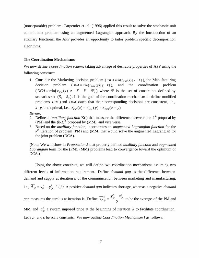
Using the above construct, we will define two coordination mechanisms assuming two

different levels of information requirement. Define demand gap as the difference between

demand and supply at iteration k of the communication between marketing and manufacturing,

i.e., kijt

kijt

kijt yx −=δ , ∀i,j,t. A positive demand gap indicates shortage, whereas a negative demand

gap measures the surplus at iteration k. Define 2

kijt

kijtk

ijt

xyxy

+= to be the average of the PM and

MM, and kijtq a system imposed price at the beginning of iteration k to facilitate coordination.

Let ε , ρ and c be scale constants. We now outline Coordination Mechanism I as follows:

18

(Coordination Mechanism I)

Iteration k+1

Step 1: The PMs and MMs solve their corresponding decision problem using their own

objective function along with the system-imposed transfer pricing:

The Marketing Problem (PMs solve)

Xto subject

xcqxyxz

Minimize

Mi Fj Ttijt

kijt

kijt

Mi Fj Tt

kijtijtPM

∈

++−+ ∑∑∑∑∑∑∈ ∈ ∈∈ ∈ ∈

x

x )(2/)()( 2 δε (7)

The Manufacturing Problem (MMs solve)

Yto subject

ycqxyyz

Minimize

Mi Fj Ttijt

kijt

kijt

Mi Fj Tt

kijtijtMM

∈

+−−+ ∑∑∑∑∑∑∈ ∈ ∈∈ ∈ ∈

y

y )(2/)()( 2 δε (8)

Step 2: Update the transfer prices as follows:

TtFjMiqqkijt

kijt

kijt ∈∈∈∀+=

++ ,,11 δρ

If the proposals from PM and MM are consistant (x=y)than terminate, otherwise k ← k+1.

Mechanism I is designed based on the principle of a price based decomposition algorithm. The

interconnecting decision variables between PM and MM are relaxed while the manufacturing

and marketing subproblems are coordinated via non- linear prices which account for

disagreement in their earlier quantity proposals. The total cost of the transfer (prices times

quantities) at any iteration is added as a cost term to the marketing problem and as a revenue

term to the manufacturing problem. What differentiates this algorithm from a classical dual

decomposition is the additional quadratic terms which penalize the deviation of common

decision variables from their average in the previous iteration and the linear penalty term which

penalizes the demand gap. Both terms can be interpreted as the bargaining power of one party

over to the other for decreasing the demand gap in their favor. The quadratic term in Mechanism

I reflects the assumption that the bargaining power of both sides are equal. The term could be

modified to reflect an inbalanced bargaining power of the participants and the algorithm retains

the same analytical properties. For example consider the following quadratic penalty terms.

19

∑∑∑∈ ∈ ∈

+−

Mi Fj Tt

kijt

kijt

ijt

xyx ε2/

3

22

∑∑ ∑∈ ∈ ∈

+−

Mi Fj Tt

kijt

kijt

ijt

xyy ε2/

32

2

The above terms would reflect a more influencial manufacturing division that can induce the

other side to make more sacrifice from their proposals to come to an agreement. The

coordination mechanism allows managers of either sides to estimate the decisions of the other

side using the information revealed in the previous iteration. This information can be a fixed

(historic) value throughout the iterations, rather than a dynamic value that changes at every

iteration and the analytical properties of the algorithm will be the same. This type of application

would be more applicable when decision makers have accurate and detailed historic information

about each other before the negotiation starts. Note that the price update in Step 2 requires

globally available information (i.e., the previous price set and the quantity proposals), which

need to be tracked at a designated central location in a transparent way. Also note that the

mechanism may terminate with some of the prices being negative, indicating that the capacity

seller (MM) has to pay for them to the capacity buyer (PM). This is due to the fact that the MMs

has a utilization target below which a penalty incurs in their local problem. Occasionally, it may

be less costly for MM to produce more than the PMs’ demands rather than operating at low

capacity utilization.

Proposition 5 Mechanism I solves an Augmented Lagrangian function of model DCA. The

sequence of (proposals, transfer prices) vectors is bounded and it converges to a saddle point of

the associated augmented lagrangian function with the appropriate choice of scale parameters.

Proof. We first define Mechanism I using the following notation and show that the mechanisms

indeed achieve the optimum of DCA at convergence. The decision vectors x, y represent the

decision variables associated with the marketing and the manufacturing problems, respectively.

X and Y represent the feasible sets for x and y. Further, define

yxu ∪= the complete decision vector associated with DCA

YXU ∪= the feasible set for vector u

J(u)= the objective function of DCA, zDCA

20

Θ(u)= the consistency measure (i.e., tjiyx ijtijt ,,,∀− )

k = the iteration index

For problem (DCA), define an augmented Lagrangian function as follows: 2

c ||)T (||2/)T ( , )(J),(L uuququu

)( + ⟩⟨+=∈

cU

where the operator ⟩⟨ , denotes inner product, and q is the price vector.

Using the following auxiliary function, Mechanism I allows the PM (the MM) problem to

measure the difference between its current proposal and the kth proposal by MM (the PM):

∑∑∑∑∑∑∈ ∈ ∈∈ ∈ ∈

−+−=Mi Fj Tt

kijtijt

Mi Fj Tt

kijtijt xyyx 2/)(2/)()K( 22u

Thus, we may reduce the Coordination Mechanism I to the following APP algorithm for (DCA):

Algorithm APP

1)T ( update

solve

)T (),T (ec)T (,e),(Ke)eJ()K( min

1

1

'

+←+=

⇒

⟩⟨+⟩⟨+⟩⟨−++

+

+

∈

kkqq

q

kkk

k

kk

U

u

u

uuuuuuu k

u

ρ

Where K′(.) is the derivative of K(.). Since the specific auxiliary function K(.) is separable by

the MM and PM problems, Algorithm APP and Mechanism I are in fact equivalent. This could

be easily verified by substituting functions Θ(u), K(u) and J(u) as defined. As proved in (Cohen

and Zhu (1984)), algorithm APP converges to a saddle point (u*,q*) of Lc(u,q) with the

appropriate choice of scale parameters. Thus, Mechanism I finds the optimum of DCA at

convergence o

Proposition 5 shows that Mechanism I is in essence a decentralized implementation of APP

where PM and MM independently solve their portion of the objective function J(u) and auxiliary

function K(u), while communicating their differences via the consistency measure Θ(u).

Importantly, the decentralized implementation does not require either side to reveal their local

problem explicitly. Nonetheless, Mechanism I does require the two sides exchange detailed

information on their solutions. This could be problematic since this level of information

exchange may not be practical, especially when the dimension of the solution vector (defined by

technologies, facilities, and periods) is high. To address this issue, we propose an alternative

coordination mechanism that requires communication at more aggregate level. Specifically, we

21

define Coordination Mechanism II as follows which communicates the aggregated demand and

capacity information with each other.

(Coordination Mechanism II)

Iteration k+1

Step 1. The PMs and MMs solve their corresponding decision problem as follows using

their own objective function along with the system-imposed transfer pricing:

The Marketing Problem (PMs solve)

Xto subject

xcq

exbxz

Minimize

Mi Fj Ttijt

kijt

kijt

Fj Tt

kjt

Miijt

Mi Fj Tt

kijtijtPM

∈

++

−+−+

∑∑∑

∑∑ ∑∑∑∑

∈ ∈ ∈

∈ ∈ ∈∈ ∈ ∈

x

x

)(

2/)(2/)()( 22

δ

εε

kijt

Mm

kijt

kjt

kijt

Mi

kijt

kjt xxebandye

where

+−== ∑∑∈∈

)(

The Manufacturing Problem (MMs solve)

Yto subject

ycq

dypyz

Minimize

Mi Fj Ttijt

kijt

kijt

Mi Tt Fj

kitijt

Mi Fj Tt

kijtijtMM

∈

+−

−+−+

∑∑∑

∑∑ ∑∑∑∑

∈ ∈ ∈

∈ ∈ ∈∈ ∈ ∈

y

y

)(

2/)(2/)()(22

δ

εε

kijt

Ff

kijt

kit

kijt

Fj

kijt

kit yydpandxd

where

+−== ∑∑∈∈

)(

Step 2: Update prices as below.

TtFjMiqqkijt

kijt

kijt ∈∈∈∀+=

++ ,,11 δρ

If proposals agree than terminate else k ← k+1

The quadratic terms in Mechanism II penalize the common decisions as they deviate from the

aggregate supply and aggregate demand proposed in the previous iteration. We will refer to the

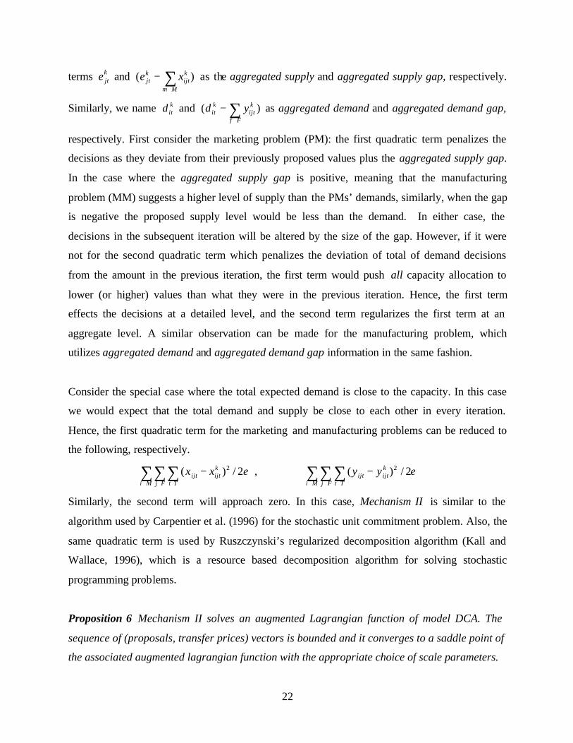
22

terms kjte and )( ∑

∈

−Mm

kijt

kjt xe as the aggregated supply and aggregated supply gap, respectively.

Similarly, we name kitd and )( ∑

∈

−Ff

kijt

kit yd as aggregated demand and aggregated demand gap,

respectively. First consider the marketing problem (PM): the first quadratic term penalizes the

decisions as they deviate from their previously proposed values plus the aggregated supply gap.

In the case where the aggregated supply gap is positive, meaning that the manufacturing

problem (MM) suggests a higher level of supply than the PMs’ demands, similarly, when the gap

is negative the proposed supply level would be less than the demand. In either case, the

decisions in the subsequent iteration will be altered by the size of the gap. However, if it were

not for the second quadratic term which penalizes the deviation of total of demand decisions

from the amount in the previous iteration, the first term would push all capacity allocation to

lower (or higher) values than what they were in the previous iteration. Hence, the first term

effects the decisions at a detailed level, and the second term regularizes the first term at an

aggregate level. A similar observation can be made for the manufacturing problem, which

utilizes aggregated demand and aggregated demand gap information in the same fashion.

Consider the special case where the total expected demand is close to the capacity. In this case

we would expect that the total demand and supply be close to each other in every iteration.

Hence, the first quadratic term for the marketing and manufacturing problems can be reduced to

the following, respectively.

∑∑∑∈ ∈ ∈

−Mi Fj Tt

kijtijt xx ε2/)( 2 , ∑∑ ∑

∈ ∈ ∈

−Mi Fj Tt

kijtijt yy ε2/)( 2

Similarly, the second term will approach zero. In this case, Mechanism II is similar to the

algorithm used by Carpentier et al. (1996) for the stochastic unit commitment problem. Also, the

same quadratic term is used by Ruszczynski’s regularized decomposition algorithm (Kall and

Wallace, 1996), which is a resource based decomposition algorithm for solving stochastic

programming problems.

Proposition 6 Mechanism II solves an augmented Lagrangian function of model DCA. The

sequence of (proposals, transfer prices) vectors is bounded and it converges to a saddle point of

the associated augmented lagrangian function with the appropriate choice of scale parameters.

23

The proof for Proposition 6 is similar to that of Proposition 5 where we can view the mechanism

as a special implementation of the Auxiliary Problem Principle by choosing the appropriate

auxiliary functional. Similar to Mechanism I, a constant aggregate demand and supply

estimation can be used throughout Mechanism II iterations. In contrast to Mechanism I, the

aggregated demand and capacity information is more likely to be available from historical data.

In general, the information requirements for Mechanism II is lower than that of Mechanism I.

4. Computational Study

We divide the computational study into two parts. First, we construct a numerical example to

illustrate the coordination mechanism and to gain some insights on their convergence behavior.

Next, we construct and solve a real-world capacity allocation problem using actual data obtained

from a major US semiconductor manufacturer.

4.1. Numerical example

We consider a 4-technology, 2-facility and 2-period example, where 4×2×2=16 common

decision variables need to be coordinated between PM and MM. We consider 6 demand

scenarios and 6 yield scenarios, and all scenarios have equal probability of occurrence. The

resulting (DCA) model has 348 variables and 192 constraints. We identify two cases where in

(Case 1) the total capacity meets the expected demands, and in (Case 2) the capacity is

significantly below that of the expected demands. More specially, for Case 1 (Case 2) the total

expected demand over all technologies is set to 100% (130%) of the total capacity over all

facilities. Both cases are common in the semiconductor industry: Case 1 represents a more stable

operating environment typical for more mature products, whereas Case 2 represents the demand

surge during a ramp-up period typical for new products. In the former case, coordination is

relatively easier since there are ample capacity, while in the later case both PMs and MMs need

to make sacrifices from their locally optimized solutions and share the burden from excess

demand. The complete numerical data is given in the Appendix. The data set is generated

following the same methodology used in Karabuk and Wu (1999).

24

In implementing both of the mechanisms, we set the augmented Lagrangian penalty parameter c

to zero so as to simplify the comparison. The c parameter is designed for nonconvex objectives

(Cohen Zhu 1984). Since our example problem is linear quadratic, exclusion of the c parameter

should not make significant difference. Pilot runs confirm this to be the case.

4.1.1. (Case 1): Mature Products- When the Capacity Meets the Total Expected Demand

We perform pilot runs on sample data to find the appropriate ε and ρ values. Parameter ρ

influence the rate at which the transfer prices are updated in each iteration, and parameter ε

determines the weight of the quadratic penalty terms, which regulates the effects of the price

updates and enhances convergence. For the numerical example at hand it turned out that ρ ∈ (0,

1.0] coupled with ε equal to 1/ρ ensures convergence. Any combination of (ε, ρ) values obtained

this way could be a good starting point for further experimentation in a general setting.

As a result of the pilot study, we use (ε=10, ρ=0.1) and (ε=12, ρ=0.1) for Mechanisms I and II

respectively. Note the increase in ε for Mechanism II essentially decreases the influence of the

quadratic penalty term in the mechanism. This is because in Mechanism II the information

communicated between the subproblems is set at a more aggregate level, which reduces the

overall inconsistency between the subproblem solutions, and the needs to regulate the price

updates. The mechanism stops when the Euc lidian distance between the x=(xijt) and y=(yijt)

vectors is below a threshold value of 16 (the number of common decision variables). To generate

feasible solutions for comparison, at the termination of each mechanism we compute the mean of

the x and y vectors as input to the model (DCA). These decisions are fixed and the (DCA) model

is solved (by adjusting the inventory I and outsourcing O levels) to compute the objective values

of the two mechanisms. Table 1 summarizes the parameter settings and performance of the two

algorithms. The last column indicates the percent deviation of the algorithm’s solution from the

global optimum, which is obtained by solving DCA directly.

Table 1. Summary of algorithm settings and performance for Case 1.

Method ε ρ Iteration # Soln. % deviation

Mechanism I 10 0.1 66 302,754 0.14%

Mechanism II 12 0.1 38 302,816 0.16%

25

The results show that both mechanisms converge to within 0.2% of the optimal solution. The

deviation from optimum is likely to be the result of round off errors. In terms of performance, it

takes Mechanism II a smaller number of iterations to converge compared to Mechanism I. This is

somewhat surprising because Mechanism II uses information in an aggregated level compared to

Mechanism I. However, recall from the discussion in Section 3.3 that in the special case where

the total expected demand is close to the capacity, the aggregated demand and supply

information used in Mechanism II will be close to each other early on in the iterations. The

example under Case 1 demonstrated this situation. Figure 1 shows the convergence plot of the

two mechanisms. One important observation from the Figure is that the gap between subproblem

solutions reduces to a low level quite early (around 22 for Mechanism II, and 31 for Mechanism

I) and improves very slowly after that. This suggests that a good heuristic solution could be

obtained by terminating the iterations early.

Convergence Plot Case (i )

0

20004000

60008000

100001200014000

160001800020000

1 4 7 10 13 16 19 22 25 28 31 34 37 40 43 46 49 52 55 58 61 64

Iterations

Dis

tanc

e

Algorithm1 Algorithm2

Figure 1. Convergence plot for Case 1

4.1.2. (Case 2): New Products- When the Capacity is Below the Total Expected Demand

Table 2 summarizes the parameter settings and performance of the algorithms for Case 2. Similar

to Case 1 both algorithms converges to the optimum. However, this time Mechanism I converge

faster than Mechanism II. In Case 2 the degree of conflict between the subproblems is higher due

Mechanism I Mechanism II

26

to the excess demand and Mechanism I solves the problem effectively by using more aggressive

parameter settings. Nevertheless, the performance of Mechanism II is quite close to that of

Mechanism I and is certainly acceptable.

Table 2. Summary of algorithm settings and performance: Case 2

Method ε ρ Iteration # Soln. % deviation

Mechanism I 4 0.25 43 384,600 0.01%

Mechanism II 12 0.10 56 384,806 0.07%

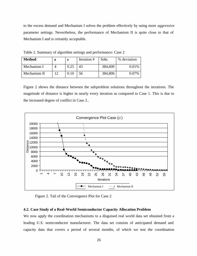
Figure 2 shows the distance between the subproblem solutions throughout the iterations. The

magnitude of distance is higher in nearly every iteration as compared to Case 1. This is due to

the increased degree of conflict in Case 2..

Convergence Plot Case (i i )

02000

400060008000

10000

120001400016000

1800020000

1 4 7 10 13 16 19 22 25 28 31 34 37 40 43 46 49 52 55

Iterations

Dis

tanc

e

Algorithm1 Algorithm2

Figure 2. Tail of the Convergence Plot for Case 2

4.2. Case Study of a Real-World Semiconductor Capacity Allocation Problem

We now apply the coordination mechanisms to a disguised real world data set obtained from a

leading U.S. semiconductor manufacturer. The data set consists of anticipated demand and

capacity data that covers a period of several months, of which we test the coordination

Mechanism I Mechanism II

27

mechanism over a period of 4 weeks. The data set contains completed demand and capacity

scenarios over the planning horizon, as well as cost data such as the underage and overage

penalty for production deviations, and the underutilization penalty. Due to a confidentiality

agreement we are not able to present the actual data set, but we will discuss the characteristics of

the data set as follows. 55 aggregate technologies are cons idered for capacity planning. The firm

has five semiconductor fabs located worldwide. Each time bucket for capacity allocation is one

week over a planning horizon of one month. The expected total demand for the planning horizon

is 10% above the total available capacity. The unit production cost for a technology can be

different at different facilities due to managerial and physical factors such as the age of the

facility. The demand for products using mature technologies is relatively steady and the

manufacturing process has relatively little variability. On the other hand, products requiring new

technologies are typically in the process of ramping up, which have highly volatile demand and

highly variable yields (capacity). Included in the dataset are 20 demand scenarios and 20

capacity scenarios. Besides demand and capacity, the inventory carrying and outsourcing (or

lost sales) costs also depend on particular products and technologies. Products that are more

commodity- like has relatively lower inventory carrying costs since excess production is more

likely to sell in future periods. On the other hand, custom products made for specific customers

are more sensitive to specification changes and excess production is likely to be scrapped. This

result in a higher inventory carrying costs. Further, for custom products the firm maybe the only

supplier for the customer and outsourcing may not be possible. Capacity shortage in these cases

would result in loss of sales. On the other hand, there are products which demands are managed

via consignment where the supplier owns and keeps track of the inventory at the customer’s site.

In such arrangements, there is usually a safety stock against possible shortages and shortage

during a single period does not have immediate effect on the customer’s production. Outsourcing

cost in the later case would be relatively insignificant.

We apply Mechanism I and Mechanism II to the above data set which would produce a solution

corresponding to DCA. However, due to the size of the problem, it is computationally infeasible

to solve the theoretical benchmark, the JCA model. For both of the mechanisms, we set the

augmented Lagrangean penalty parameter c to zero for the same reasons we stated in the

previous section. The appropriate ε and ρ values turned out to be (ε=0.5, ρ=0.5) and

28

(ε=1, ρ=0.01) with Mechanism I and Mechanism II respectively. In comparison with the small

example of the previous subsection, the ε has been reduced, thus increasing the magnitude of the

quadratic penalty term. This adjustment led to a higher ρ value in Mechanism I and a smaller ρ

for Mechanism II. This difference is because subproblems in Mechanism I are regulated better

and more aggressive price adjustments are possible. However, Mechanism II, using aggregate

information in the regularizing terms of the subproblems requires small adjustments in the prices

to converge. This causes Mechanism II to converge slower.

The mechanisms are stopped when the Euclidean distance between the x=(xijt) and y=(yijt)

vectors is below a threshold value of 1100 (the number of common decision variables). Table 3

summarizes the parameter settings and performance of the two algorithms.

Table 3. Summary of mechanism settings and performance

Method ε ρ Iteration #

Mechanism I 0.5 0.5 75

Mechanism II 1 0.01 423

Figure 3 shows the convergence plots of the two mechanisms. As one would expect, Mechanism

I converges faster than Mechanism II due to more detailed information it utilizes throughout the

iterations. Mechanism II on the other hand requires only aggregated information to pass between

the problems. In decision-making environments where both parties agree to supply the detailed

information that is needed by Mechanism I to each other, it should be the natural choice to

facilitate coordination. On the other hand, in an environment where the decision-makers consider

their detailed proposals private information and react only to prices announced by a mutually

agreed mediator, Mechanism II may be the only applicable choice. In our example of the

semiconductor manufacturer, it is most likely that both PMs and MMs would be more

comfortable only with passing aggregate information during the iterations. In that case, it will not

be possible to identify a single manager who performs poorly. However, this case study shows

the potential improvements in the negotiation process if such detailed information is made

available to the decision-makers.

29

Convergence Plot - Real World Data

0

5000

10000

15000

20000

25000

30000

35000

40000

1 51 101 151 201 251 301 351 401Iterations

Dis

tanc

e

Algorithm 1 Algorithm 2

Figure 3. Convergence plot for the mechanisms applied to actual data.

5. Conclusion

In this paper, we study the issues of decentralizing capacity planning decision in the

semiconductor industry. Using the general framework of stochastic programming, we model the

decision problem using the viewpoints from the marketing managers, the manufacturing

managers, and the firm. We first show that decentralization requires the additional restriction of

maintaining private information, which creates unavoidable degradation on overall performance.

Under the private information assumption, we show that coordination is achievable between

marketing and manufacturing using an information exchange scheme. We propose two

coordination mechanisms using this scheme and proof that the mechanism will converge to the

global solution as defined by model DCA. From a mathematical standpoint, we modeled the

information exchange as a nonlinear component added to the local objective function of

competing decision-makers. This component reflects the amount of information that one

decision-maker has about the other side and regulates the local decisions to match to the other

side more closely. We proved the convergence of this information exchange scheme using the

Auxiliary Problem Principle (APP). The APP theory provides a flexible analytical framework to

develop coordination mechanisms. The two mechanisms we developed in this study are only

Mechanism I Mechanism II

30

examples among a wide variety of possibilities. Finally, we demonstrate the working of the

proposed mechanisms using generated numerical data and a real world data set.

Acknowldegement This research is supported in part by the National Science Foundation grant DMI-9634808 and a research grant from Lucent Technologies. References Burton, R.M., and Obel, B., 1980, "The efficiency of the price, budget, and mixed approaches under varying a priori information levels for decentralized planning", Management Science, Vol. 26, No.4. Berman, O., and Ganz, Z., and Wagner, J.M., 1994, "A stochastic optimization model for planning capacity expansion in a service industry under uncertain demand", Naval Research Logistics, Vol. 41, pp. 545-564. Bertsekas, Dimitri P., 1996, “Constrained optimization and lagrangean multiplier methods”, Athena Scientific, Belmont, Massachusetts. Bienstock, D., and Shapiro, J.F., 1988, "Optimizing resource acquisition decisions by stochastic programming", Management Science, Vol. 34, No.2. Carpentier, P., and Cohen, G., and Culioli, J.-V., 1996, "Stochastic optimization of unit commitment: a new decomposition framework", IEEE Transactions on Power Systems, Vol. 11, No. 2. Christensen, J., and Obel, B., 1978, "Simulation of decentralized planning in two Danish organizations using linear programming decomposition", Management Science, Vol.24, No.15. Cohen, Guy, 1978, “Optimization by decomposition and coordination: a unified approach”, IEEE Transactions on Automatic Control, Vol. AC-23, No. 2. Cohen, G. and Zhu, D. L. 1984, “Decomposition coordination methods in large scale optimization problems: the nondifferentiable case and the use of augmented lagrangians”, in Advances in Large Scale Systems Theory and Applications, Vol. 1, J.B. Cruz ed., JAI Press, Greenwich, Connecticut. Cohen, Guy and Miara, Bernadette, 1990, “Optimization with an auxiliary constraint and decomposition”, SIAM Journal on Control and Optimization, Vol.28, No.1, pp.137-157.

31

Culioli, J.-C and Cohen, G., 1990, “Decomposition/Coordination algorithms in stochastic optimization”, SIAM J. Control and Optimization, Vol. 28, No. 6, pp.1372-1403. Dantzig, G.B., and Wolfe, P., 1961, "The Decomposition Algorithm for Linear Programs", Econometrica, Vol. 29, No.4. Eppen, G.D., and Martin, R.K., and Schrage, L., 1989, "A scenario approach to capacity planning", Operations Research, Vol 37, No. 4. Ertogral, K., and Wu, S.D., 1999, “Auction-Theoretic Coordination of Production Planning in the Supply Chain”, Lehigh University, Department of Industrial and Manufacturing Systems Engineering, Report No. 99T-01. Escudero, L. F., and Kamesam, P., and V., King, A., J., and Wets, R. J-B., 1993, "Production planning via scenario modeling", Annals of Operations Research, 43, pp.311-335. Jennergren, P., 1972, "Decentralization on the basis of price schedules in linear decomposable resource allocation Problems", Journal of Financial and Quantitative Analysis. Jose, R.A., Harker, P.T., and Ungar, L.H., 1997, “Auctions and optimization: methods for closing the gap caused by discontinuities in demands”, Technical Report, University of Pennsylvania. Kall, P. and Wallace, S.W., 1994, Stochastic Programming, Wiley-Interscience Series in Systems and Optimization. Karabuk S., and Wu, S.D., 1999, “Strategic Capacity Planning in the Semiconductor Industry: A Stochastic Programming Approach”, Lehigh University, Department of Industrial and Manufacturing Systems Engineering, Report No. 99T-12. Kate, T., 1972, "Decomposition of Linear Programs by Direct Distribution", Econometrica, Vol. 40, No.5. Kouvelis, P. and Martin A. Lariviere, 2000, “Decentralizing Cross-Functional Decisions: Coordination Through Internal Markets,” Management Science 46, 1049-1058. Kutanoglu, E and Wu, S.D., 1999, “On combinatorial auction and Lagrangean relaxation for distributed resource scheduling”, IIE Transactions, vol.31, no.9, pp.813-26. Luna, H.P.L., 1984, "A survey on Informational Decentralization and Mathematical Programming Decomposition", Mathematical Programming, R.W. Cottle, M.L., Kelmanson and B.Korte (Editors), Elsevier Science Publishers. Mulvey, J.M. and Ruszczynski, A., 1995, "A New Scenario Decomposition Method for Large-Scale Stochastic Optimization", Operations Research, No.3.

32

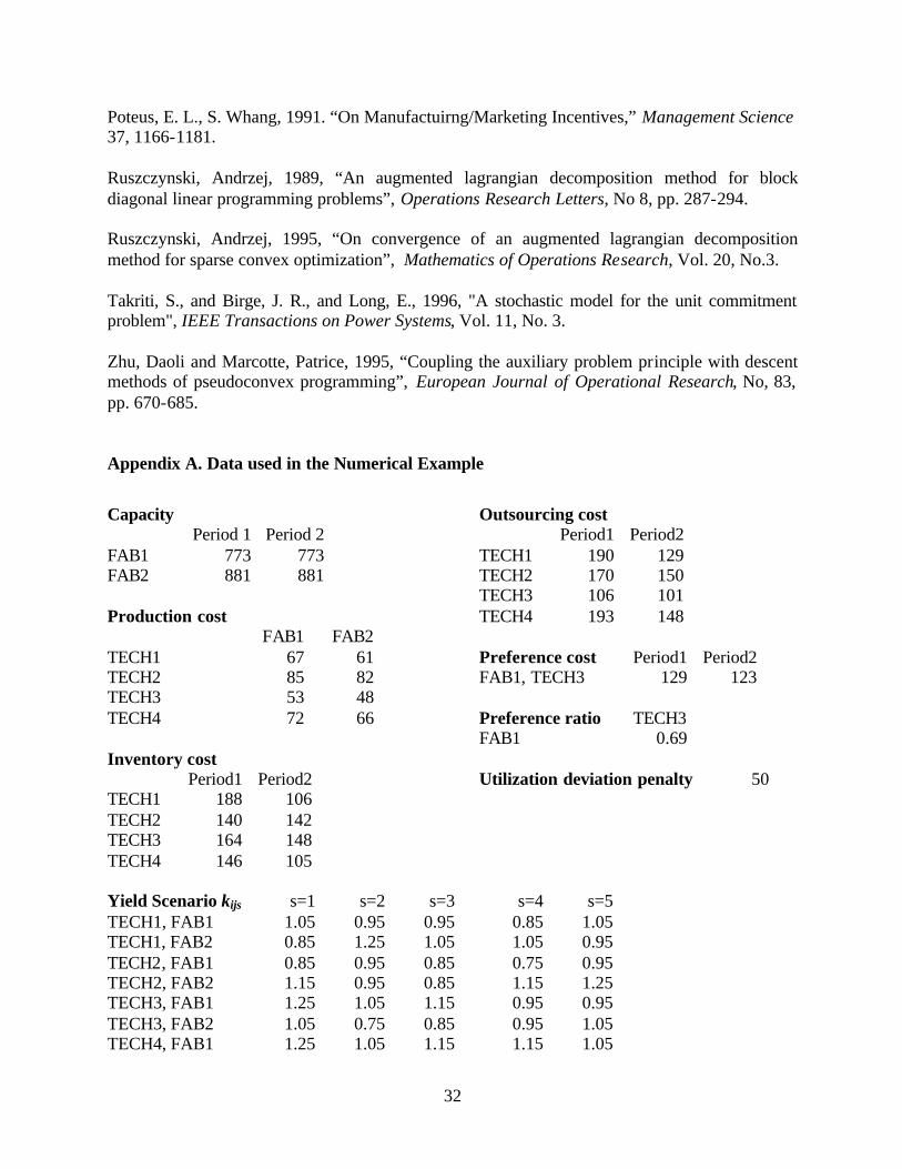
Poteus, E. L., S. Whang, 1991. “On Manufactuirng/Marketing Incentives,” Management Science 37, 1166-1181. Ruszczynski, Andrzej, 1989, “An augmented lagrangian decomposition method for block diagonal linear programming problems”, Operations Research Letters, No 8, pp. 287-294. Ruszczynski, Andrzej, 1995, “On convergence of an augmented lagrangian decomposition method for sparse convex optimization”, Mathematics of Operations Research, Vol. 20, No.3. Takriti, S., and Birge, J. R., and Long, E., 1996, "A stochastic model for the unit commitment problem", IEEE Transactions on Power Systems, Vol. 11, No. 3. Zhu, Daoli and Marcotte, Patrice, 1995, “Coupling the auxiliary problem principle with descent methods of pseudoconvex programming”, European Journal of Operational Research, No, 83, pp. 670-685. Appendix A. Data used in the Numerical Example

Capacity

Period 1 Period 2 FAB1 773 773 FAB2 881 881 Production cost

FAB1 FAB2TECH1 67 61TECH2 85 82TECH3 53 48TECH4 72 66 Inventory cost

Period1 Period2 TECH1 188 106 TECH2 140 142 TECH3 164 148 TECH4 146 105

Outsourcing cost

Period1 Period2 TECH1 190 129 TECH2 170 150 TECH3 106 101 TECH4 193 148 Preference cost Period1 Period2 FAB1, TECH3 129 123 Preference ratio TECH3 FAB1 0.69 Utilization deviation penalty 50

Yield Scenario kijs s=1 s=2 s=3 s=4 s=5 TECH1, FAB1 1.05 0.95 0.95 0.85 1.05 TECH1, FAB2 0.85 1.25 1.05 1.05 0.95 TECH2, FAB1 0.85 0.95 0.85 0.75 0.95 TECH2, FAB2 1.15 0.95 0.85 1.15 1.25 TECH3, FAB1 1.25 1.05 1.15 0.95 0.95 TECH3, FAB2 1.05 0.75 0.85 0.95 1.05 TECH4, FAB1 1.25 1.05 1.15 1.15 1.05

33

TECH4, FAB2 0.85 1.15 1.05 0.75 1.15 Demand Scenario dits

s=1 s=2 s=3 s=4 s=5 s=6

TECH1, PERIOD1 567.00 513.00 621.00 621.00 621.00 513.00 TECH1, PERIOD2 498.10 615.30 673.90 498.10 615.30 615.30 TECH2, PERIOD1 535.50 637.50 433.50 382.50 484.50 586.50 TECH2, PERIOD2 575.70 757.50 696.90 636.30 575.70 696.90 TECH3, PERIOD1 352.50 446.50 446.50 446.50 446.50 493.50 TECH3, PERIOD2 541.65 353.25 400.35 541.65 494.55 494.55 TECH4, PERIOD1 680.80 503.20 562.40 503.20 680.80 503.20 TECH4, PERIOD2 640.55 584.85 417.75 529.15 640.55 529.15

This data represents case 2. Case 1 data is obtained by dividing all demand values by 1.3.

34

WHY THIS PAPER IS RELEVENT

This paper examines a decentralized coordination scheme in the setting of semiconductor

capacity planning: marketing managers reserve capacity from manufacturing based on product

demands, while attempting to maximize profit; manufacturing managers allocate capacity to

competing marketing managers so as to minimize operating costs while ensuring efficient

resource utilization. Using the general framework of stochastic programming, we model the

decision problem using the viewpoints from the marketing managers, the manufacturing

managers, and the firm. We first show that decentralization requires the additional restriction of

maintaining private information, which creates unavoidable degradation on overall performance.

Under the private information assumption, we show that coordination is achievable between

marketing and manufacturing using an information exchange scheme. We propose two

coordination mechanisms using this scheme and proof that the mechanism will converge to the

global solution. We demonstrate the working of the proposed mechanisms using generated

numerical data and a real world data set.

This paper is relevant in that it provides an novel view of cross-functional decision making that

integrate different viewpoints in an internal market. The model also brings out important

connection between optimization/algorithmic insights, and organizational decision structure.

Our findings suggest that decentralized coordination are achievable but come at a cost, but in

terms of performance and communication overhead. These tradeoffs are quantifiable and should

be carefully analyzed by decision makers.