RESEARCH ARTICLE

Decay of passive-scalar fluctuations in slightly stretchedgrid turbulence

S. K. Lee • A. Benaissa • L. Djenidi •

P. Lavoie • R. A. Antonia

Received: 8 November 2011 / Revised: 17 May 2012 / Accepted: 22 May 2012 / Published online: 14 June 2012

� Springer-Verlag 2012

Abstract Isotropic turbulence is closely approximated by

stretching a grid flow through a short (1.36:1) secondary

contraction. The flow is operated at small values of the

Taylor microscale Reynolds number (about 25–55) and is

slightly heated just downstream of the grid, so that the

temperature serves as a passive scalar and the initial

velocity/thermal length-scale ratio is about 1. For the same

grid, the contraction reduces the skewness and kurtosis of

the thermal fluctuations and their derivative. The thermal

fluctuations and their mean dissipation rates follow a

power-law rate of decay that depends on the geometry of

the grid. Comparison with velocity measurements shows

that, for three different grids, the ratio between the tem-

perature and velocity power-law exponents closely mat-

ches the velocity/thermal timescale ratio. For the present

measurements, the timescale ratio is slightly larger than 1

but does not exceed 1.2, in accordance with the proposal by

Corrsin (J Aeronaut Sci 18(6):417–423, 1951b).

1 Introduction

The decay in grid-generated turbulence has been the sub-

ject of extensive research since the work of Taylor (1935b).

Grid turbulence is of interest because it represents a close

approximation to homogeneous isotropic turbulence. The

similarity analysis of this flow (e.g. Karman and Howarth

1938; Dryden 1943; Batchelor 1953) allows testing of the

concept of universal behaviour of turbulence. While it is

well accepted that, in grid turbulence, the decay of the

turbulent kinetic energy, q02 (a prime denotes the root-

mean-square value), follows a power law q02� tnq , where

nq \ 0, the actual value of nq has yet to be established.

There are currently two different theories for predicting nq.

The first theory by Batchelor and Proudman (1956) indi-

cates nq = -10/7, and the second theory by Saffman

(1967) predicts nq = -6/5. In reality, measurements of nq

are rather sensitive to different grid flows, and this makes it

difficult to test the theories. In fact, the variability of nq

(from near -1 to -1.5 reported in literature) has led to the

notion that nq may not be universal at finite Reynolds

numbers (e.g. George 1992a, b; George et al. 2001). There

are very few measurements, perhaps only those of Lavoie

et al. (2007) and Krogstad and Davidson (2010), where

large number of velocity data points are collected over a

wide downstream range in an attempt to more accurately

determine the decay rate (nq).

Lavoie (2006) has established that the variation in nq

mainly arises from different initial conditions (i.e. grid

geometry and Reynolds number) that affect the character-

istics of the turbulence. These characteristics, for example,

include the intensity of vortex shedding behind the grid, the

anisotropy of the flow and the shape of the energy spec-

trum. Strong vortex shedding and large anisotropy tend to

shift the turbulent energy to lower wavenumbers and

increase the magnitude of nq. By carefully modifying the

grid, the intensity of vortex shedding may be reduced. To

improve the isotropy of the flow, an effective method is to

S. K. Lee (&) � L. Djenidi � R. A. Antonia

School of Engineering, University of Newcastle, Newcastle,

NSW 2308, Australia

e-mail: soon-kong.lee@newcastle.edu.au

A. Benaissa

Faculty of Engineering, Royal Military College of Canada,

Kingston, ON K7K 7B4, Canada

P. Lavoie

Institute for Aerospace Studies, University of Toronto,

Toronto, ON M3H 5T6, Canada

123

Exp Fluids (2012) 53:909–923

DOI 10.1007/s00348-012-1331-3

place a smooth contraction downstream of the grid (e.g.

Comte-Bellot and Corrsin 1966). The purpose of a con-

traction is to stretch the flow (e.g. Prandtl 1933; Taylor

1935b), so that the ratio of streamwise to cross-stream

velocity fluctuations is more approximately closer to one

(e.g. Uberoi 1956). The combined effect of a more iso-

tropic flow and a less intense vortex shedding reduces both

the magnitude of nq and the dependence of nq on the initial

conditions (Lavoie et al. 2007).

For this study, our focus is on scalar fluctuations because

the mixing of scalar quantities is at the core of phenomena

such as dispersion of pollutants, combustion and air con-

ditioning. The particular interest here is on the decay of

temperature fluctuations in grid turbulence which is more

nearly isotropic, that is, grid flows slightly stretched by a

secondary contraction (Comte-Bellot and Corrsin 1966;

Lavoie et al. 2007). The temperature is introduced, so that

it can be treated as a ‘‘passive’’ scalar, where it has no

dynamical effect on the flow. For mixing in isotropic tur-

bulence, George (1992a) and Antonia et al. (2004) have

indicated that both the scalar spectrum equation and the

scalar transport equation satisfy similarity if the scalar

variance h02 decays as a power law h02� tnh , where nh \ 0.

Since the work began with Corrsin (1951a, b) and co-

workers (e.g. Mills et al. 1958; Mills and Corrsin 1959),

there are rather fewer studies on the scalar decay rate (nh)

than there are on the velocity decay rate (nq). Of the more

relevant experimental studies, mainly by Warhaft and co-

workers, and recent progress in modelling scalar fluctua-

tions in homogeneous/grid turbulence, notably by Viswa-

nathan and Pope (2008), we shall briefly discuss here.

Warhaft and Lumley (1978) have shown that nh is

sensitive to the initial conditions of the flow but also

depends on the method of heating. By directly heating the

grid, nh and the shape of the temperature spectrum are

strongly affected by the intensity of the thermal fluctua-

tions, h02=DT2, where DT is the temperature difference

across the grid. For a fixed Reynolds number, increasing

the power to heat the grid shifts the temperature spectrum

to lower wavenumbers and increases the magnitude of nh.

This may be avoided by heating the flow either down-

stream of the grid with an array of fine wires—known as a

‘‘mandoline’’ (e.g. Warhaft and Lumley 1978; Warhaft

1980)—or upstream in the plenum with an array of wire

ribbons—known as a ‘‘toaster’’ (e.g. Sirivat and Warhaft

1983). Both methods of heating, unlike grid heating, pro-

duce better cross-stream homogeneity in the thermal field.

However, with the mandoline technique, h02 is independent

of the action of turbulence production, and the velocity/

thermal timescale ratio tends to be closer to unity (i.e. nh/nq

& 1.4) than that obtained by using a toaster (nh/nq & 1.6)

(Sirivat and Warhaft 1983). Also, with the mandoline, it is

easier to control the initial scale of the temperature fluc-

tuations independently of their fluctuation intensity; this is

done by adjusting the spacing between the wires and/or the

distance of the mandoline from the grid. Typically, the

diameter of the heater wires is very fine (no more than

0.5 mm), and the heating is small enough (temperature

difference DT . 8 �C) to avoid physical or thermal wake

disturbance to the velocity field (e.g Warhaft and Lumley

1978; Sreenivasan et al. 1980; Warhaft 1984).

From their experiments in active-grid turbulence,

Mydlarski and Warhaft (1996, 1998) indicated that,

although the passive-scalar field may be mixed and

advected by an approximately isotropic velocity field, the

two fields generally do not behave the same. For example,

at small Reynolds numbers, the scalar spectrum has a more

discernible power-law scaling range than the velocity

spectrum. By increasing the Reynolds number, the power-

law exponent for the scaling range approaches the

Kolmogorov value of ‘‘-5/3’’ more rapidly for the scalar

than for the velocity. As suggested by Mydlarski and

Warhaft (see also Warhaft 2000), the difference may reflect

some dissimilarity in the morphology of the two fields

other than the possible effects due to the method of heating

(i.e. scalar boundary condition).

In their Lagrangian modelling of scalar fluctuations in

grid turbulence, Viswanathan and Pope (2008) applied a

modified form of the IECM (see Sawford 2004) that takes

into account the effect of molecular diffusion; the model is

carefully developed, so that it is consistent with prescribed

Eulerian velocity statistics, and it requires the specification

of a timescale ratio. They tested single/multiple (up to 4)

line sources and heated mandoline and obtained a good

match with the experimental results of Warhaft and Lumley

(1978) and Warhaft (1984). From their model, Viswanathan

and Pope (2008) verified two important experimental

observations. (1) The scalar (h02) decay rate depends on the

spacing between sources in the mandoline with respect to

the integral turbulence (velocity) length scale. (2) At large

downstream distances from the mandoline, the scalar decay

rate (when plotted against distance from the mandoline)

does not depend on the scalar/velocity length-scale ratio.

We note that, for the experimental data used to verify their

model, the location of the mandoline is (at least) 20 mesh

lengths downstream of the grid, the magnitude of the scalar

decay rate is rather large, for example nh = -2.06 (the

streamwise-velocity decay rate is nu = -1.34), and this

reflects the large timescale ratio nh/nu = 1.5, which they

have selected for their modelling. The experiments of

Warhaft and Lumley (1978), Zhou et al. (2000, 2002) and

Antonia et al. (2004) have shown that, by placing the

mandoline just (1.5 mesh lengths) downstream of the grid,

the timescale ratio is closer to unity (i.e. 1.0 \ nh/nu \ 1.2).

910 Exp Fluids (2012) 53:909–923

123

In a later section, we discuss measurements of the scalar

decay rate (in the context of the length-scale ratio) and

compare them with those predicted by the Langrangian

dispersion theory (Durbin 1980, 1982)—that which was

used in the (initial) development of turbulent mixing models

such as those by Sawford and Hunt (1986), Sawford (2004)

and Viswanathan and Pope (2008).

In the light of the above discussion, it is pertinent to

begin by accurately measuring the thermal decay rate (nh)

and compare it with the velocity decay rate (nq) for grid

flows that are more closely isotropic. This paper presents

measurements of temperature fluctuations for three differ-

ent grid flows that are slightly heated with a mandoline

located immediately downstream of the grid. The purpose

of having the mandoline near the grid is so that the initial

scale of the temperature fluctuations is more closely mat-

ched to the initial integral (turbulence) length scale. This is

the first attempt to more accurately determine nh in grid

turbulence by using a large number of data points (27 in

each batch) collected over a reasonably large downstream

range (between 20 and 100 mesh lengths from the grid).

The present work extends that of Lavoie et al. (2007) on

measurements of velocity fluctuations for the same grid

flows with the aim of testing the effect of different grid

geometries on the decay rate(s) when the turbulence is

more closely isotropic at the large scales. The improvement

in isotropy is achieved primarily by stretching the longi-

tudinal vorticity component of the grid flow by using a

secondary contraction (Uberoi 1956; Comte-Bellot and

Corrsin 1966; Lavoie 2006; Lavoie et al. 2007; Antonia

et al. 2010). This paper includes measurements of skew-

ness and kurtosis of thermal fluctuations to provide some

indication of the degree of anisotropy. The work concludes

with a discussion on the length-scale and timescale ratios in

the context of the scalar and velocity decay rates for the

case of small Reynolds and Peclet numbers (Corrsin

1951b). Details of the experimental apparatus are given in

Sect. 3. The following Sect. 2 starts by describing the two

different methods used to determine the decay rate.

2 Methods to determine the decay rate

2.1 The ‘‘power-law’’ method

Homogeneous isotropic turbulence is the least complex

form of turbulence and is approximated experimentally in

the decaying velocity and thermal fluctuations downstream

of a grid. Since there is no mean shear and hence no pro-

duction of turbulent kinetic energy, the turbulence in this

flow simply decays. Many studies (e.g. Comte-Bellot

and Corrsin 1966; Mohamed and LaRue 1990; Lavoie

et al. 2007) have shown that the decay of the turbulent

kinetic energy (defined here as q02 ¼ u02 þ v02 þ w02) fol-

lows a power law:

q02� x� xoð Þnq() u02� x� xoð Þnu ; ð1Þ

where xo is the virtual origin for the grid turbulence. For

isotropic turbulence, q02 should have the same decay

exponent as u02, that is nq = nu \ 0. When a passive scalar

is introduced, the scalar variance h02, like the velocity

variance u02, also decays as a power law (e.g. Sreenivasan

et al. 1980; George 1992a; Zhou et al. 2002; Antonia et al.

2004):

h02�ðx� xhoÞ

nh ; ð2Þ

where xoh is the scalar virtual origin and nh \ 0. By

assuming Taylor’s hypothesis (i.e. x = tUo, where Uo is the

free-stream velocity), the relations (1) and (2) could

equally be expressed in terms of decay time:

q02� t � toð Þnq() u02� t � toð Þnu ; ð3Þ

h02�ðt � thoÞnh : ð4Þ

2.2 The ‘‘lambda’’ method

George et al. (2001) and Antonia et al. (2004) have shown

that an important consequence of the power laws (1) and

(2) or equivalently (3) and (4) is the linear relation for the

Taylor microscale (k) and the Corrsin microscale (kh) for

isotropic turbulence (assuming Taylor’s hypothesis), viz.

k2� � mnq

t � toð Þ ¼ � mnu

t � toð Þ; ð5Þ

k2h� �

jnhðt � thoÞ; ð6Þ

where the time derivative of the microscales (dk2/dt and

dk2h=dt) should be constant; m and j are the kinematic

viscosity and the thermal diffusivity of air, respectively.

The time derivative of the relations (5) and (6) can avoid

the need to select an arbitrary curve-fitting range to

determine the decay exponents (e.g. George et al. 2001;

Antonia et al. 2004).

3 Experimental apparatus

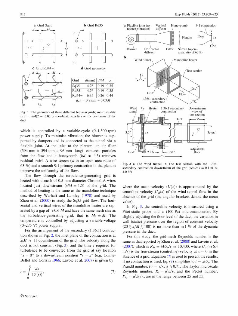
Figure 1 shows the three different biplanar grids previously

used by Lavoie et al. (2007) and Antonia et al. (2010). The

first (Sq35) is a grid of square bars with a solidity ratio (r)

of 0.35, the second (Rd35) is a grid of round bars

(r = 0.35), and the third (Rd44w) is a grid of round bars

with wire wrapped around each bar (r = 0.44). The mesh

size of each turbulence-generating grid is M = 24.76 mm.

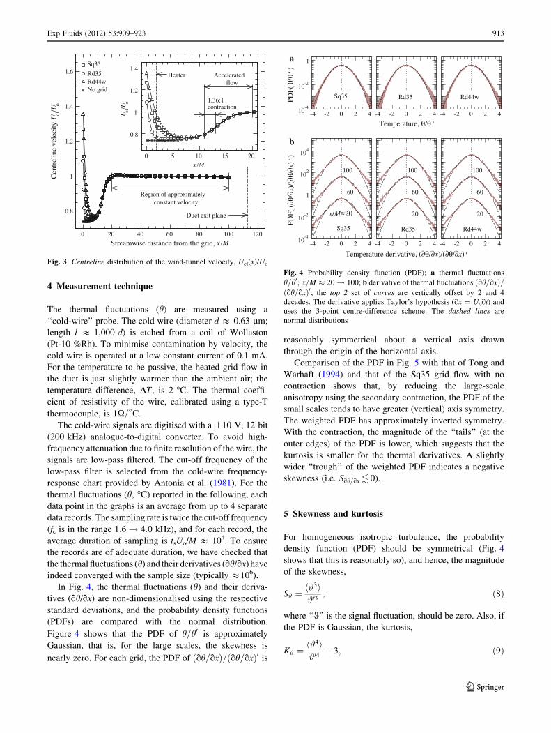
Figure 2 shows a schematic diagram of the open-circuit

wind tunnel. The air flow is driven by a centrifugal blower,

Exp Fluids (2012) 53:909–923 911

123

which is controlled by a variable-cycle (0–1,500 rpm)

power supply. To minimise vibration, the blower is sup-

ported by dampers and is connected to the tunnel via a

flexible joint. At the inlet to the plenum, an air filter

(594 mm 9 594 mm 9 96 mm long) captures particles

from the flow and a honeycomb (l/d & 4.3) removes

residual swirl. A wire screen (with an open area ratio of

63 %) and a smooth 9:1 primary contraction in the plenum

improve the uniformity of the flow.

The flow through the turbulence-generating grid is

heated with a mesh of 0.5-mm diameter Chromel-A wires

located just downstream (x/M = 1.5) of the grid. The

method of heating is the same as the mandoline technique

described by Warhaft and Lumley (1978) and used by

Zhou et al. (2000) to study the Sq35 grid flow. The hori-

zontal and vertical wires of the mandoline heater are sep-

arated by a gap of &0.6 M and have the same mesh size as

the turbulence-generating grid, that is Mh = M. The

temperature is controlled by adjusting a variable-voltage

(0–275 V) power supply.

For the arrangement of the secondary (1.36:1) contrac-

tion shown in Fig. 2, the inlet plane of the contraction is at

x/M & 11 downstream of the grid. The velocity along the

duct is not constant (Fig. 3), and the time t required for

turbulence to be convected from the grid at say location

‘‘s = 0’’ to a downstream position ‘‘s = x’’ (e.g. Comte-

Bellot and Corrsin 1966; Lavoie et al. 2007) is given by

t ¼Zx

0

ds

hUðsÞi ; ð7Þ

where the mean velocity hUðxÞi is approximated by the

centreline velocity Ucl(x) of the wind-tunnel flow in the

absence of the grid (the angular brackets denote the mean

value).

In Fig. 3, the centreline velocity is measured using a

Pitot-static probe and a (100-Pa) micromanometer. By

slightly adjusting the floor level of the duct, the variation in

wall (static) pressure over the region of constant velocity

(20. x=M. 100) is no more than &1 % of the dynamic

pressure in the duct.

For this study, the grid-mesh Reynolds number is the

same as that reported by Zhou et al. (2000) and Lavoie et al.

(2007), which is RM = MUo/m & 10,400, where Uo (&6.4

m/s) is the free-stream (centreline) velocity at x = 0 in the

absence of a grid. Equation (7) is used to present the results;

if no contraction is used, Eq. (7) simplifies to t = x/Uo. The

Prandtl number, Pr = m/j, is &0.71. The Taylor microscale

Reynolds number, Rk ¼ u0k=m, and the Peclet number,

Pkh ¼ u0kh=j, are in the range between 25 and 55.

0.8 mm 0.03M

Grid Md / σd(mm)

Sq35Rd35Rd44w

4.764.766.35

0.190.190.26

0.350.350.44

Grid Rd44w

Grid Rd35Grid Sq35 ba

Grid geometrydc

dwd

d

∼∼dwd =

x

d M

M x

d

y

z

x

M+dwd

Fig. 1 The geometry of three different biplanar grids; mesh solidity

is r = d/M(2 - d/M); x coordinate axis lies on the centreline of the

duct

1.36:1 secondarycontraction

xzy

Grid

Wind tunnel

Test section

Mandoline heater

z

yx

Duct

l3.5

l3

3l+

test sectionview of

ytunnel

DownstreamWind Heater

Δl

contraction1.36:1 secondary

l282.72l 0.51lGrid floor

Adjustable

Flow

b

ay

xFlow

area ratio of 63%)Blower Filter

9:1 contraction

Horizontal

Honeycombreduce vibration) diffuser

Screen (open−

Flexible joint (to Vertical

diffuser

Grid

Plenum

Fig. 2 a The wind tunnel. b The test section with the 1.36:1

secondary contraction downstream of the grid (scale: l = 0.1 m &4.0 M)

912 Exp Fluids (2012) 53:909–923

123

4 Measurement technique

The thermal fluctuations (h) are measured using a

‘‘cold-wire’’ probe. The cold wire (diameter d & 0.63 lm;

length l & 1,000 d) is etched from a coil of Wollaston

(Pt-10 %Rh). To minimise contamination by velocity, the

cold wire is operated at a low constant current of 0.1 mA.

For the temperature to be passive, the heated grid flow in

the duct is just slightly warmer than the ambient air; the

temperature difference, DT , is 2 �C. The thermal coeffi-

cient of resistivity of the wire, calibrated using a type-T

thermocouple, is 1X=�C.

The cold-wire signals are digitised with a ±10 V, 12 bit

(200 kHz) analogue-to-digital converter. To avoid high-

frequency attenuation due to finite resolution of the wire, the

signals are low-pass filtered. The cut-off frequency of the

low-pass filter is selected from the cold-wire frequency-

response chart provided by Antonia et al. (1981). For the

thermal fluctuations (h, �C) reported in the following, each

data point in the graphs is an average from up to 4 separate

data records. The sampling rate is twice the cut-off frequency

(fc is in the range 1:6! 4:0 kHz), and for each record, the

average duration of sampling is tsUo/M & 104. To ensure

the records are of adequate duration, we have checked that

the thermal fluctuations (h) and their derivatives (qh/qx) have

indeed converged with the sample size (typically &106).

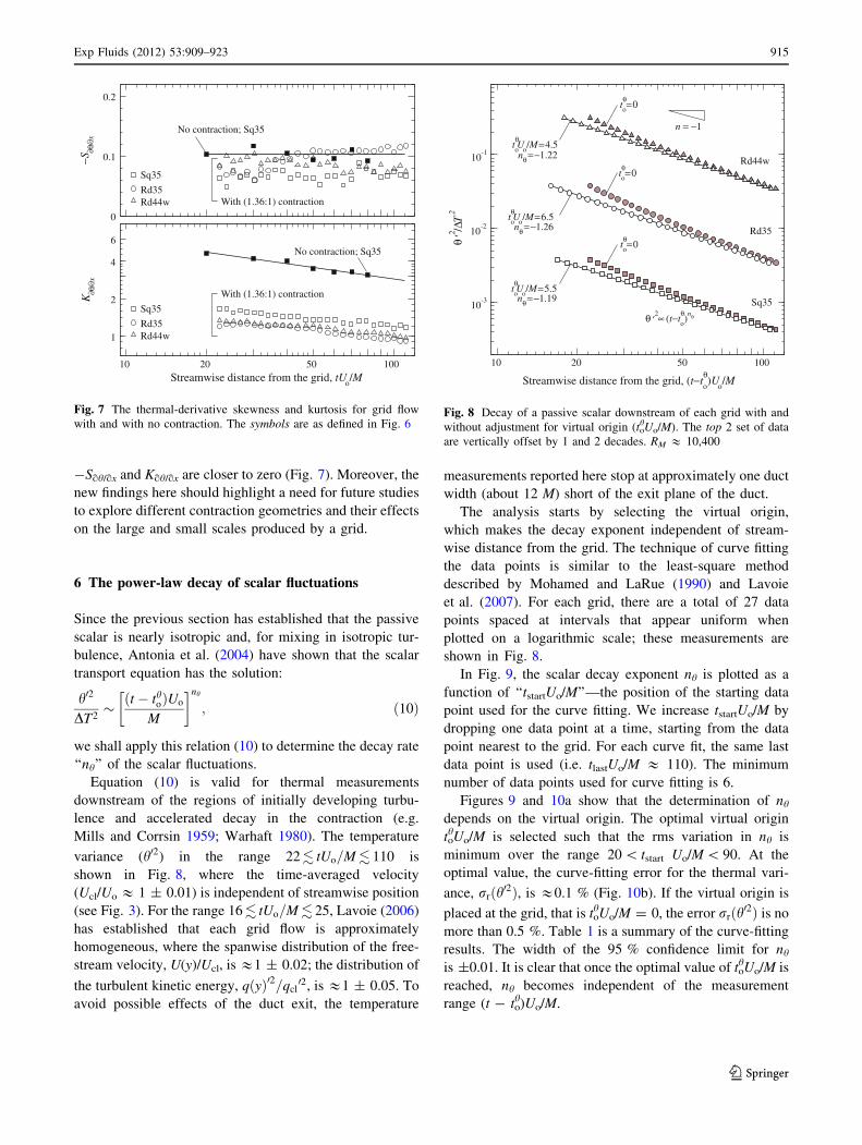
In Fig. 4, the thermal fluctuations (h) and their deriva-

tives (qh/qx) are non-dimensionalised using the respective

standard deviations, and the probability density functions

(PDFs) are compared with the normal distribution.

Figure 4 shows that the PDF of h=h0 is approximately

Gaussian, that is, for the large scales, the skewness is

nearly zero. For each grid, the PDF of ðoh=oxÞ=ðoh=oxÞ0 is

reasonably symmetrical about a vertical axis drawn

through the origin of the horizontal axis.

Comparison of the PDF in Fig. 5 with that of Tong and

Warhaft (1994) and that of the Sq35 grid flow with no

contraction shows that, by reducing the large-scale

anisotropy using the secondary contraction, the PDF of the

small scales tends to have greater (vertical) axis symmetry.

The weighted PDF has approximately inverted symmetry.

With the contraction, the magnitude of the ‘‘tails’’ (at the

outer edges) of the PDF is lower, which suggests that the

kurtosis is smaller for the thermal derivatives. A slightly

wider ‘‘trough’’ of the weighted PDF indicates a negative

skewness (i.e. Soh=ox. 0).

5 Skewness and kurtosis

For homogeneous isotropic turbulence, the probability

density function (PDF) should be symmetrical (Fig. 4

shows that this is reasonably so), and hence, the magnitude

of the skewness,

S# ¼h#3i#03

; ð8Þ

where ‘‘0’’ is the signal fluctuation, should be zero. Also, if

the PDF is Gaussian, the kurtosis,

K# ¼h#4i#04� 3; ð9Þ

400 20 60 80 100 120

Streamwise distance from the grid, x /M

0.8

1

1.2

1.4

1.6

Cen

trel

ine

velo

city

, Ucl

/Uo

Region of approximatelyconstant velocity

Duct exit plane

Sq35

Rd35Rd44wNo grid

0 5 10 15 20x /M

0.8

1

1.2

1.4

U cl/U

o

Accelerated

contraction1.36:1

flowHeater

Fig. 3 Centreline distribution of the wind-tunnel velocity, Ucl(x)/Uo

-4 -2 0 2 410

-4

10-2

1

102

104

PDF(

(∂θ

/∂x)

/(∂θ

/∂x)’

)

Sq35

b

x/M 20

60

100

~~

-4 -2 0 2 4

Temperature derivative, (∂θ/∂x)/(∂θ/∂x)’

Rd35

20

60

100

-4 -2 0 2 4

Rd44w

20

60

100

-4 -2 0 2 410-4

10-2

1

PDF(

θ/θ’

)

a

Sq35

-4 -2 0 2 4

Temperature, θ/θ’

Rd35

-4 -2 0 2 4

Rd44w

Fig. 4 Probability density function (PDF); a thermal fluctuations

h=h0; x=M � 20! 100; b derivative of thermal fluctuations ðoh=oxÞ=ðoh=oxÞ0; the top 2 set of curves are vertically offset by 2 and 4

decades. The derivative applies Taylor’s hypothesis (qx = Uoqt) and

uses the 3-point centre-difference scheme. The dashed lines are

normal distributions

Exp Fluids (2012) 53:909–923 913

123

should be zero. However, grid turbulence only approxi-

mates isotropic turbulence, and its weighted PDF is

not strictly symmetrical and is not Gaussian (see Figs. 4

and 5). Therefore, a departure from zero skewness and

zero kurtosis should serve as a measure of flow anisotropy

for the majority of large (0 : h) and small (0 : qh/qx)

scales.

In Fig. 6, the thermal skewness Sh and the kurtosis Kh

are nearer to zero for the square-bar grid (Sq35) than for

the round-bar grids (Rd35 and Rd44w); Sh and Kh are

largest for grid Rd35. This suggests that the large scales

produced by the square-bar grid are weaker than those

produced by the round-bar grids. This is consistent with

Lavoie’s (2006) deduction from his hydrogen-bubble flow

visualisation, where a square-bar grid produces mainly

‘‘anti-phase’’ vortex shedding that tends to breakdown the

large scales; a round-bar grid produces mainly ‘‘in-phase’’

vortex shedding that tends to sustain the large scales.

Figure 6 clearly shows a dependence of large-scale motion

on the different grids. Since Fig. 7 shows that the three

grids produce nearly identical trends in the thermal-deriv-

ative skewness Sqh/qx and the kurtosis Kqh/qx, the small-

scale motion has a weak dependence on the geometry of

the grids.

A comparison of the thermal skewness Sh in Fig. 6 with

that of Mills et al. (1958) shows that the combined effect of

the secondary contraction, the wire wrapping of the round

bars (Rd44) and a lower heating temperature (reducing DT

from about 5 to 2 �C) produces a more constant skewness

(Rd44w: Sh & 0.05). Without a secondary contraction, the

Sq35 grid flow has a negative skewness (Sh & -0.02) and

a larger kurtosis (Kh & 0.23).

Antonia et al. (1978) have reported that, for a grid flow

not stretched by a contraction, the skewness and the

kurtosis of the thermal derivatives are somewhere in

the ranges �0:34. Soh=ox. 0:05 and 2.Koh=ox. 7. The

thermal-derivative kurtosis (Kqh/qx) reported by Antonia

et al. (1978) are subtracted by ‘‘3’’, so that their results are

consistent with Eq. (9). Their thermal measurements

(x=M � 29! 115; RM � 20;200; Rk � 40; DT � 5 �C) are

obtained with a grid of round bars at 36 % solidity that

closely matches the present grid Rd35. Inspection of Fig. 7

shows that the contraction keeps the magnitude of the

thermal-derivative skewness small (i.e. |Sqh/qx| \ 0.2) and

reduces the thermal-derivative kurtosis (Kqh/qx) by a factor

of (up to) about 3. For grid Sq35, the magnitudes for both

-Sqh/qx and Kqh/qx are smaller with the contraction than

with no contraction.

From the evidence above, we conclude that, for a fixed

grid (Sq35) with the (1.36:1) secondary contraction, the

passive scalar is more nearly isotropic at both the large

scales (h) and the small scales (qh/qx). Although Sh and Kh

are small (\0.3), the effect of grid geometry on the large

scales is not negligible. The small scales are much less

sensitive to the grid and, with the secondary contraction,

the improvement in isotropy is obvious, that is, the PDF

of ðoh=oxÞ=ðoh=oxÞ0 is more nearly Gaussian (Fig. 5), and

10-5

10-4

100

101

PDF(

ϑ)a

(1994); no contrac.

Sq35; with contrac.Sq35; no contrac.Tong and Warhaft

-12 -9 -6 -3 0 3 6 9 12

ϑ = (∂θ/∂x)/(∂θ/∂x)’

-0.4

0

0.4

ϑ3 × PD

F(ϑ)

Gaussian

b

Fig. 5 PDF for a square-bar grid flow with and without the (1.36:1)

contraction. The normal distributions are shown as dashed lines. The

data (open square) of Tong and Warhaft (1994) are for a square-bargrid of 34 % solidity; x/M = 62; RM = 9,700; Rk = 38

-0.1

0

0.1

Skew

ness

, Sθ

Rd35

(Rd44)

Rd44w

Sq35

No contraction; Sq35

10 20 50 100

Streamwise distance from the grid, tUo/M

0.1

0.2

0.3

Kur

tosi

s, K

θ

No contraction; Sq35

Rd35

Sq35

Rd44w

Fig. 6 The thermal skewness and kurtosis for grid flow with the

1.36:1 contraction (open square Sq35, open circle Rd35, opentriangle Rd44w) and with no contraction (filled square Sq35). For the

Rd44 data (dashed lines) of Mills et al. (1958) (a round-bar gridof 44 % solidity; x=M � 15! 80; RM � 7; 000; Rk � 19! 26;DT � 5 �C), the grid flow is with no contraction. The solid curvesare a visual guide

914 Exp Fluids (2012) 53:909–923

123

-Sqh/qx and Kqh/qx are closer to zero (Fig. 7). Moreover, the

new findings here should highlight a need for future studies

to explore different contraction geometries and their effects

on the large and small scales produced by a grid.

6 The power-law decay of scalar fluctuations

Since the previous section has established that the passive

scalar is nearly isotropic and, for mixing in isotropic tur-

bulence, Antonia et al. (2004) have shown that the scalar

transport equation has the solution:

h02

DT2� ðt � thoÞUo

M

� �nh

; ð10Þ

we shall apply this relation (10) to determine the decay rate

‘‘nh’’ of the scalar fluctuations.

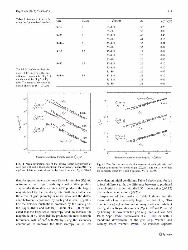
Equation (10) is valid for thermal measurements

downstream of the regions of initially developing turbu-

lence and accelerated decay in the contraction (e.g.

Mills and Corrsin 1959; Warhaft 1980). The temperature

variance (h02) in the range 22. tUo=M. 110 is

shown in Fig. 8, where the time-averaged velocity

(Ucl/Uo & 1 ± 0.01) is independent of streamwise position

(see Fig. 3). For the range 16. tUo=M. 25, Lavoie (2006)

has established that each grid flow is approximately

homogeneous, where the spanwise distribution of the free-

stream velocity, U(y)/Ucl, is &1 ± 0.02; the distribution of

the turbulent kinetic energy, qðyÞ02=qcl02, is &1 ± 0.05. To

avoid possible effects of the duct exit, the temperature

measurements reported here stop at approximately one duct

width (about 12 M) short of the exit plane of the duct.

The analysis starts by selecting the virtual origin,

which makes the decay exponent independent of stream-

wise distance from the grid. The technique of curve fitting

the data points is similar to the least-square method

described by Mohamed and LaRue (1990) and Lavoie

et al. (2007). For each grid, there are a total of 27 data

points spaced at intervals that appear uniform when

plotted on a logarithmic scale; these measurements are

shown in Fig. 8.

In Fig. 9, the scalar decay exponent nh is plotted as a

function of ‘‘tstartUo/M’’—the position of the starting data

point used for the curve fitting. We increase tstartUo/M by

dropping one data point at a time, starting from the data

point nearest to the grid. For each curve fit, the same last

data point is used (i.e. tlastUo/M & 110). The minimum

number of data points used for curve fitting is 6.

Figures 9 and 10a show that the determination of nh

depends on the virtual origin. The optimal virtual origin

tohUo/M is selected such that the rms variation in nh is

minimum over the range 20 \ tstart Uo/M \ 90. At the

optimal value, the curve-fitting error for the thermal vari-

ance, rrðh02Þ, is &0.1 % (Fig. 10b). If the virtual origin is

placed at the grid, that is tohUo/M = 0, the error rrðh02Þ is no

more than 0.5 %. Table 1 is a summary of the curve-fitting

results. The width of the 95 % confidence limit for nh

is ±0.01. It is clear that once the optimal value of tohUo/M is

reached, nh becomes independent of the measurement

range (t - toh)Uo/M.

0

0.1

0.2−S

∂θ/∂

x

No contraction; Sq35

With (1.36:1) contraction

Sq35

Rd35Rd44w

10 20 50 100Streamwise distance from the grid, tU

o/M

1

2

4

6

K∂θ

/∂x

No contraction; Sq35

With (1.36:1) contraction

Sq35

Rd35Rd44w

Fig. 7 The thermal-derivative skewness and kurtosis for grid flow

with and with no contraction. The symbols are as defined in Fig. 6

10 20 50 100

Streamwise distance from the grid, (t−tθo)U

o/M

10-3

10-2

10-1

θ’2 /Δ

T2

tθo=0

tθo=0

tθo=0

θ’2∝(t−tθo)nθ

n = −1

Sq35

Rd35

tθoU

o/M=5.5

nθ=−1.19

nθ=−1.26

nθ=−1.22Rd44w

tθoU

o/M=6.5

tθoU

o/M=4.5

Fig. 8 Decay of a passive scalar downstream of each grid with and

without adjustment for virtual origin (tohUo/M). The top 2 set of data

are vertically offset by 1 and 2 decades. RM & 10,400

Exp Fluids (2012) 53:909–923 915

123

7 Mean dissipation rate and the Corrsin microscale

In this section, we determine the decay rate nh by analysing

the mean dissipation rate hvdi and the Corrsin microscale

kh. In Fig. 11, hvdi is approximated by the streamwise

decay rate of h02. The formula is taken from the statistical

analysis of grid turbulence by Zhou et al. (2002):

hvdiMUoDT2

¼ � 1

2

d h02=DT2� �d x=Mð Þ : ð11Þ

Each data point shown in Fig. 11 is calculated by using the

3-point centre-difference scheme and then averaged over

its two closest points. To avoid end effects due to the

scheme, the outer 2 points on each end of a batch of 27 data

points are removed. To obtain a power-law expression for

hvdi, we substitute (10) into (11) and use Taylor’s

hypothesis, viz.

hvdiMUoDT2

� � nh

2

t � tho� �

Uo

M

� �nh�1

: ð12Þ

In Fig. 11, the rms difference between the data points

and the power law (12) is no more than 0.5 %. Given that

hvdi, like h02, reasonably follows a power-law decay, we

may write the following expression for kh (after Corrsin

1951b; Monin and Yaglom 1975; George 1992a):

kh2

M2¼ 6j

M2

h02

hvdi¼ � 12j

nhMUo

t � tho� �

Uo

M: ð13Þ

Equation (13) shows that kh2 is a linearly increasing

function of (t - toh)Uo/M, and the measurements in

Fig. 12 support this. It follows that dk2h=dt should be

constant and this can be used to estimate nh, viz.

kh2

M t � tho� �

Uo

¼ � 12jnhMUo

: ð14Þ

The term on the left side of Eq. (14) is plotted in Fig. 13 as

a function of tUo/M. The virtual origin tohUo/M is selected

such that kh2=½M t � tho

� �Uo� and nh are constant for the full

range of measurements.

The results, summarised in Table 2 and Fig. 14, show

that the ‘‘lambda’’ method yields nearly the same virtual

origin (tohUo/M) and decay exponent (nh) as those obtained

by the ‘‘power-law’’ method. However, the lambda method

uses a centre-difference scheme, where the number of

useful data points are reduced from 27 to 23, which slightly

increases the width of the 95 % confidence limit for nh

from ±0.01 to ±0.02. At the optimal tohUo/M, the curve-

fitting error for the mean dissipation rate, rrðhvdiÞ, is

&0.2 %. If tohUo/M = 0, the error rrðhvdiÞ is no more than

0.5 %. Adjusting tohUo/M by ±0.5 changes nh by no more

than ±0.02.

8 Discussion on the decay rates

Table 3 provides a review summary of the available mea-

surements from the present wind tunnel. The results show

-1.3

-1.1Sq35

Incr

easi

ngde

cay

rate

10.0

tθoU

o/M = 0

5.5

-1.4

-1.2

Dec

ay e

xpon

ent f

or te

mpe

ratu

re f

luct

uatio

ns, n

θ

tθoU

o/M = 0

10.0 Rd35

6.5

10 20 50 100

tstart

Uo/M

-1.3

-1.1Rd44w10.0

tθoU

o/M = 0

4.5

Fig. 9 Decay exponent nh as a function of the starting position tstart

for the curve-fitting range ftstart ! tlastg and the virtual origin tohUo/

M. The position of the last data point is fixed at tlast Uo/M & 110. The

error bars are for 95 % confidence limits

20 50 100 150

tstart

Uo/M

0

0.5

σ r(θ’2 ),

(%

)

Grid tθoU

o/M

b

Sq35 0

Rd35 0Rd44w 0Sq35 5.5

Rd35 6.5Rd44w 4.5

0 2 4 6 8 10 12

tθoU

o/M

0

1

2

3

σ r(nθ),

(%

)

Rd44w

Rd35

Sq35

a

Fig. 10 a The root-mean-square (rms) variation in the decay

exponent (nh: 20 \ tstart Uo/M \ 100 in Fig. 9) as a function of

virtual origin tohUo/M. b The rms curve-fitting error for the scalar

variance (h02 in Fig. 8) as a function of tstart and toh for the curve-fitting

range ftstart ! tlastg, where tlast Uo/M & 110

916 Exp Fluids (2012) 53:909–923

123

that, for approximately the same Reynolds number (Rk) and

optimum virtual origin, grids Sq35 and Rd44w produce

very similar thermal decay rates; Rd35 produces the largest

magnitude of the thermal decay rate. With the contraction,

the effect of grid geometry is rather weak and the differ-

ence between nh produced by each grid is small (.0:07).

For the velocity fluctuations produced by the same grids

(i.e. Sq35, Rd35 and Rd44w), Lavoie et al. (2007) indi-

cated that the large-scale anisotropy tends to increase the

magnitude of nu (since Rd44w produces the most isotropic

turbulence with u02=w02 � 0:99); by using the secondary

contraction to improve the flow isotropy, nu is less

dependent on initial conditions. Table 3 shows that, for (up

to four) different grids, the difference between nu produced

by each grid is smaller with the 1.36:1 contraction (.0:12)

than with no contraction (.0:23).

Inspection of the results in Table 3 shows that the

magnitude of nh is generally larger than that of nu. This

trend (i.e. nhJnu) is observed in many studies of turbulent

mixing at low Reynolds numbers (RM & 103 and Rk & 35)

by heating the flow with the grid (e.g. Yeh and Van Atta

1973; Sepri 1976; Sreenivasan et al. 1980) or with a

mandoline downstream of the grid (e.g. Warhaft and

Lumley 1978; Warhaft 1980). The evidence supports

Table 1 Summary of curve fit

using the ‘‘power-law’’ method

The 95 % confidence limit for

nh is �0:01; rrðh02Þ is the rms

difference between the ‘‘log’’ of

the data and the ‘‘log’’ of Eq.

(10). The range of the curve fit

data is shown as (t - toh)Uo/M

Grid tohUo/M (t - to

h)Uo/M -nh rrðh02Þð%Þ

Sq35 0 22–110 1.35 0.25

35–80 1.35 0.08

Rd35 0 22–110 1.46 0.43

35–80 1.44 0.13

Rd44w 0 22–110 1.35 0.31

35–80 1.33 0.09

Sq35 5.5 17–110 1.19 0.08

35–110 1.20 0.04

35–80 1.20 0.05

Rd35 6.5 17–110 1.26 0.10

35–110 1.26 0.10

35–80 1.26 0.09

Rd44w 4.5 17–110 1.22 0.10

35–110 1.21 0.06

35–80 1.21 0.06

10 20 50 100

Streamwise distance from the grid, (t−tθo)U

o/M

10-6

10-5

10-4

10-3

10-2

<χd>M

/UoΔT

2

Sq35

Rd35

Rd44w

tθoU

o/M=6.5

tθoU

o/M=4.5

<χd>∝(t−t

θo)nθ−1

nθ−1 = −2.23

tθoU

o/M=5.5

nθ−1 = −2.27

nθ−1 = −2.21

tθo=0

tθo=0

tθo=0

Fig. 11 Mean dissipation rate of the passive scalar downstream of

each grid with and without adjustment for virtual origin (tohUo/M). The

top 2 set of data are vertically offset by 1 and 2 decades. RM & 10,400

10 20 50 100

Streamwise distance from the grid, (t−tθo)U

o/M

10-2

10-1

100

101

λ θ2 /M2

Rd44w

λθ2/M2∝(t−t

θo)/(−nθ)

Rd35

Sq35

tθoU

o/M=5.5

tθo=0

tθo=0

tθo=0

nθ=−1.21

tθoU

o/M=6.5

nθ=−1.27

tθoU

o/M=4.5

nθ=−1.23

Fig. 12 The Corrsin microscale downstream of each grid with and

without adjustment for virtual origin (tohUo/M). The top 2 set of data

are vertically offset by 1 and 2 decades. RM & 10,400

Exp Fluids (2012) 53:909–923 917

123

Mydlarski and Warhaft’s (1998) notion that the scalar and

velocity fields behave differently and that the difference

cannot be accounted for by the method of heating alone.

In the following Sects. 8.1 and 8.2, we discuss the dif-

ference between the scalar and velocity decay rates from

the perspective of the length-scale and timescale ratios for

small Reynolds and Peclet numbers. The ratios are

important parameters, for example, in the ‘‘calibration’’ of

numerical models to yield results that would match

experimental observations (e.g. Viswanathan and Pope

2008).

8.1 The scalar/velocity length-scale ratio

Durbin’s (1980) theory on turbulent dispersion, which is

extended from the early work of Taylor (1921, 1935a) on

the dispersion of heat from a (line) source in a turbulent air

stream, has since been adapted to model turbulent mixing

with multiple line sources and mandoline (e.g. Sawford and

Hunt 1986; Sawford 2004; Viswanathan and Pope 2008). It

is therefore fitting to provide here a brief summary of

Durbin’s (1982) findings on the scalar decay rate in iso-

tropic turbulence (in the context of length-scale ratio) and

to compare the present measurements with his model

results (reproduced in Fig. 15).

According to Durbin (1980, 1982), the rate of decay of

scalar fluctuations is largely determined by mixing due to

relative dispersion. The length scales or (by Taylor’s

hypothesis) timescales of both scalar and velocity fields are

necessary to describe the scalar decay rate nh. At low/finite

Reynolds numbers, both fields are transient and depend on

their initial scales. Durbin (1982) suggests that ‘‘the exis-

tence of two scales relaxes similarity constraints, so that a

universal decay law need not exist’’. His findings show

that, for isotropic turbulence, nh depends on lu;o=lh;oð.2:5Þ,the ratio between initial length scales for the velocity and

the scalar fluctuations. Figure 15 shows that, for the range

covered by measurements, this dependence is negligible

provided that lu,o/lh,o [ 2.5 (or lh,o/lu,o \ 0.4).

0.8

1.2

1.6

2.0 Sq35

tθoU

o/M=0

4.5

10.0

Incr

easi

ngde

cay

rate

0.8

1.2

1.6

2.0

(λθ2 /[M

(t−t

θ o)Uo])

×10

3

Rd35

tθoU

o/M=0

6.5

10.0

10 20 50 100

Streamwise distance from the grid, tUo/M

0.8

1.2

1.6

2.0 Rd44w

tθoU

o/M=0

5.5

10.0

Fig. 13 The Corrsin microscale as a function of streamwise position

and virtual origin. Equation (14) is used to obtain the decay rate nh

Table 2 Summary of curve fit using the ‘‘lambda’’ method

Grid tohUo/M (t - to

h)Uo/M -nh rrðh02Þ ð%Þ rrðhvdiÞ ð%Þ

Sq35 4.5 17–110 1.23 0.07 0.15

35–110 0.05 0.14

35–80 0.04 0.15

Rd35 6.5 17–110 1.27 0.09 0.17

35–110 0.10 0.15

35–80 0.09 0.16

Rd44w 5.5 17–110 1.21 0.08 0.21

35–110 0.07 0.17

35–80 0.07 0.18

The 95 % confidence limit for nh is ±0.02; rrðh02Þ is the rms dif-

ference between the ‘‘log’’ of the data and the ‘‘log’’ of Eq. (10);

rrðhvdiÞ is the rms difference between the ‘‘log’’ of the data and

the ‘‘log’’ of Eq. (11). The range of the curve fit data is shown as

(t - toh)Uo/M

20 50 100 150

tstart

Uo/M

0

0.5

σ r(<χ d>)

, (%

)

Grid tθoU

o/M

b

Sq35 0

Rd35 0Rd44w 0Sq35 4.5

Rd35 6.5Rd44w 5.5

8 100 2 4 6 12

tθoU

o/M

0

3

6

9

σ r(λθ2 ),

(%

)

Rd44w

Sq35

Rd35

a

Fig. 14 a The root-mean-square (rms) variation in the Corrsin

microscale (kh2: 20 \ tUo/M \ 100 in Fig. 13) as a function of virtual

origin tohUo/M. b The rms curve-fitting error for the mean dissipation

rate (hvdi in Fig. 11) as a function of tstart and toh for the curve-fitting

range ftstart ! tlastg, where tlastUo/M & 100

918 Exp Fluids (2012) 53:909–923

123

For the review experimental data shown in Fig. 15, the

grid flow is not stretched by a secondary contraction and

the spacing between the grid and the downstream mando-

line is large—up to 20 M (Warhaft and Lumley 1978) and

54 M (Sreenivasan et al. 1980). In Fig. 15, the decay rate

nh is determined by plotting the variance h02 as a function

of streamwise distance from the heat source (i.e. mando-

line). For large spacing between the grid and the mandoline

(J5M), Durbin (1982) demonstrated that, by replotting the

data versus distance from the mandoline rather than from

the grid, this slightly reduces the magnitude of nh. With the

present measurements shown in Fig. 15, the distance

between the grid and the mandoline is too small (1.5 M) to

produce a significant change in nh.

To allow direct comparison between temperature and

velocity for the present grids (Sq35, Rd35 and Rd44w) and

to compare with the review data in Fig. 15, we have

obtained simultaneous measurements of temperature (h)

and streamwise-velocity (u) fluctuations using cold and hot

wires. The cold wire is operated under the same condition

described in Sect. 4. The hot wire (diameter d & 2.50 lm;

length l & 200 d) is operated at constant temperature with

an overheat ratio of 1.5. The wires are parallel with

a (fixed) spanwise separation of 1 mm (&1.5–3.0

Kolmogorov lengths). For this test, a total of 9 points are

measured in the range 22. tUo=M. 110; by using

the same methods (Sect. 2) and procedure (Sects. 6 and 7)

with extension to velocity, we have determined that, at

90 % confidence limit, nh and nu are the same as those

reported in Table 3 (within ±0.03 for the decay exponents

and ±1 for the virtual origins).

For each present data point ‘‘9’’ shown in Fig. 15, the

length scales lh and lu are obtained by integrating the

(spatial) auto-correlation function for the temperature and

the streamwise-velocity fluctuations, respectively. This

method is the same as that described by Comte-Bellot and

Corrsin (1971) and Sreenivasan et al. (1980). The ratio of

length scales, lh/lu, is plotted as a function of tUo/M in

Fig. 16. In view of the scatter and to avoid extrapolation,

we have decided to estimate the initial length-scale ratio

lh,o/lu,o by taking the average value over the range of the

Table 3 Review of decay exponents for velocity (nu) and temperature (nh) from the same wind tunnel

References Reynolds number Virtual

origin

Decay exponent u02=w02 Grid Experimental conditions

RM 9 10-3 Rk -nu -nh

Zhou et al. (2000) 10.4 50–55 0 1.33 1.36 Not reported Sq35 No contraction; with heating; no

offset for virtual origin;

N(nu) = N(nh) = 6 (least-square

method)

Zhou et al. (2002) 6.6 34–43 1.30 1.46

Antonia et al. (2004) 10.4 40–50 1.33 1.37

Lavoie (2006) and

Lavoie et al. (2007)

10.4 43–45 7 1.06 No data 1.45 Sq35 No contraction; no heating;

N(nu) & 55 (power-law

method); Rd44w is Rd44 with

wire wrapped around each bar28–33 6 1.20 1.27 Rd35

31–37 6 1.18 1.30 Rd44w

34–39 3 1.29 1.24 Rd44

With present

temperature

measurementsa, b

10.4 40–45 5, 5.5a 1.18 1.19a, 1.23b 1.11 Sq35 With (1.36:1) contraction and

heating; N(nu) & 55 (power-law

method); NðnhÞ ¼ 22a; 23b25–30 5, 6.5a 1.21 1.26a, 1.27b 1.07 Rd35

33–35 7, 4.5a 1.09 1.22a, 1.21b 0.99 Rd44w

33–37 4 1.14 No data 1.14 Rd44

The grid and the mandoline heater are located at tUo/M = 0 and 1.5, respectively. M = Mh = 24.76 mm; DT ¼ 2 �C. The present measurements

are obtained by using a the power-law and b the lambda methods. N denotes the number of data points in the measurement range

20 \ tUo/M \ 100

40 8

Initial length-scale ratio, lu,o

/lθ,o

1

1.5

2

2.5

−nθ

Rd35

Sq35

Rd44w Warhaft and Lumley (1978)

Sreenivasan et al. (1980)

Durbin (1982)Present measurements

Fig. 15 Decay exponent nh as a function of the initial length-scale

ratio (after Durbin 1982). The solid curve is a visual guide only

Exp Fluids (2012) 53:909–923 919

123

measurements; inspection of Fig. 15 shows that this is

likely to have overestimated the values of lu,o/lh,o, but

nonetheless, the estimates are in close agreement with

Durbin’s (1982) results. The present measurements and the

data of Warhaft and Lumley (1978) and Sreenivasan et al.

(1980) fall on the same trend established by Durbin (1980,

1982); the overall agreement lends support to Durbin’s

notion that the scalar fluctuations decay is largely due to

mixing by turbulent relative dispersion.

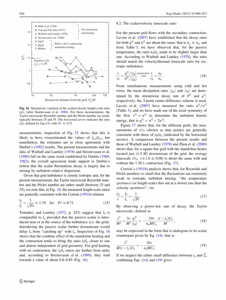
Given that grid turbulence is closely isotropic and, for the

present measurements, the Taylor microscale Reynolds num-

ber and the Peclet number are rather small (between 25 and

55), we note that, in Fig. 16, the measured length-scale ratios

are generally consistent with the Corrsin (1951b) relation

lhlu¼ 1ffiffiffiffiffi

Prp � 1:19 for Pr � 0:71: ð15Þ

Tennekes and Lumley (1972, p. 243) suggest that lh is

comparable to lu provided that the passive scalar is intro-

duced near or at the source of the turbulence (i.e. the grid).

Introducing the passive scalar further downstream would

delay lh from ‘‘catching up’’ with lu. Inspection of Fig. 16

shows that the combine effect of the mandoline heating and

the contraction tends to bring the ratio lh/lu closer to one

and almost independent of grid geometry. For grid heating

with no contraction, the lh/lu ratios are further from unity

and, according to Sreenivasan et al. (1980), they tend

towards a value of about 0.8–0.85 (Fig. 16).

8.2 The scalar/velocity timescale ratio

For the present grid flows with the secondary contraction,

Lavoie et al. (2007) have established that the decay rates

for both q02 and u02 are about the same, that is nq & nu, and

from Table 3, we have observed that, for the passive

temperature, the ratio nh/nu tends to be slightly larger than

one. According to Warhaft and Lumley (1978), this ratio

should match the velocity/thermal timescale ratio for iso-

tropic turbulence:

ssh¼ q02=hedi

h02=hvdi¼)

power laws ssh¼ nh

nu: ð16Þ

From simultaneous measurements using cold and hot

wires, the mean dissipation rates hvdi and hedi are deter-

mined by the streamwise decay rate of h02 and q02,

respectively; the 3-point centre-difference scheme is used.

Lavoie et al. (2007) have measured the ratio u02=w02

(Table 3), and we have made use of the axial symmetry of

the flow v02 ¼ w02 to determine the turbulent kinetic

energy, that is q02 ¼ u02 þ 2w02.

Figure 17 shows that, for the different grids, the mea-

surements of s/sh (shown as data points) are generally

consistent with those of nh/nu (indicated by the horizontal

arrows). A comparison between the present results and

those of Warhaft and Lumley (1978) and Zhou et al. (2000)

shows that, for a square-bar grid with the mandoline heater

located just (1.5 M) downstream of the grid, the average

timescale s/sh (&1.0 ± 0.08) is about the same with and

without the 1.36:1 contraction (Fig. 17).

Corrsin’s (1951b) analysis shows that, for Reynolds and

Peclet numbers so small that the fluctuations are extremely

weak in isotropic turbulent mixing, ‘‘the temperature

spottiness (or length scale) dies out at a slower rate than the

velocity spottiness’’, viz.

kh

k¼ lh

lu¼ 1ffiffiffiffiffi

Prp : ð17Þ

By observing a power-law rate of decay, the Taylor

microscale, defined as

k2

M2¼ 5m

M2

q02

hedi¼ � 10m

nuMUo

t � toð ÞUo

M; ð18Þ

may be expressed in the form that is analogous to its scalar

counterpart given by Eq. (14), that is

k2

Mðt � toÞUo

¼ � 10mnuMUo

: ð19Þ

If we neglect the rather small difference between to and toh,

combining Eqs. (14) and (19) gives

10 20 50 100 150

Streamwise distance from the grid, tUo/M

0.8

1

1.2

1.4

1.6

l θ/l u

grid heating

With (1.36:1) contraction;mandoline heating

No contraction;

lθ/lu = 1/√Pr

Equation (15);

Mills et al. (1958)

Yeh and Van Atta (1973)

Warhaft and Lumley (1978)

Sreenivasan et al. (1980)

Sq35

Rd35Rd44w

Fig. 16 Streamwise variation of the scalar/velocity length-scale ratio

lh/lu (after Sreenivasan et al. 1980). For these measurements, the

Taylor microscale Reynolds number and the Peclet number are small,

typically between 25 and 55. The horizontal arrow indicates the ratio

lh/lu defined by Eq.(15) with Pr & 0.71

920 Exp Fluids (2012) 53:909–923

123

nh

nuPr

kh

k

� �2

¼ 6

5: ð20Þ

By substituting Corrsin’s (1951b) relation (17) into (20),

we obtain the ratio

nh

nu¼ 1:2 ð21Þ

which is consistent with the present results (i.e. nh=nuJ1).

For the grid Rd44w that produces the most isotropic tur-

bulence (u02=w02 � 0:99), the ratio is closer to the value

prescribed by (21). From inspection of Fig. 17, we likely

suspect that the small variations in the range

1. nh=nu. 1:2 are due to initial conditions, effects of

Reynolds and Peclet numbers and non-negligible depar-

tures from isotropy.

To summarise, the present results and review data in

Figs. 15, 16 and 17 show that, by having the mandoline

located just downstream of the grid, both lh/lu and nh/nu are

very close to unity. Moving the mandoline further down-

stream of the grid increases the magnitude of lh/lu and nh/nu

(e.g. Warhaft and Lumley 1978; Warhaft 1984). For Sq35,

the 1.36:1 contraction reduces the magnitude for both nh

and nu (Table 3) although the ratio nh/nu & 1 is about the

same as that with no contraction (Fig. 17). If we strictly

observe the case of small Peclet numbers in accordance

with the proposal of Corrsin (1951b) for gaseous mixing

with Prandtl number of 0.71, the ratios lh/lu and nh/nu are

about 1.2. However, ratio nh/nu is sensitive to the initial

conditions, and so a universal value for this ratio is not

expected. Rather, nh/nu will change according to the

magnitude of nh, which depends on the initial length-scale

ratio (Fig. 15) (see also Durbin 1982).

9 Concluding remarks

This paper reports measurements of passive-scalar (tem-

perature) fluctuations in closely isotropic grid turbulence

where the length-scale and timescale ratios are about 1.

The isotropy of the large scales is obtained by slightly

stretching the flow with a short (1.36:1) contraction

(located at 11 M downstream of the grid). Three different

grids are tested for the same contraction, and the temper-

ature is introduced just (1.5 M) downstream of the grid.

The present data should be useful to assist in future vali-

dation of mixing model(s) for decaying grid turbulence

(e.g. Viswanathan and Pope 2008).

The present measurements show that the probability

density functions (PDFs) for the scalar fluctuations (h) and

their derivatives (qh/qx) are approximately symmetrical;

for the large scales, the PDFs are almost Gaussian. The

overall evidence suggests that the scalar is very nearly

isotropic. For the same grid (Sq35), the finding that the

magnitudes of the skewness and the kurtosis of the scalar

fluctuations and their derivatives are reduced with the

secondary contraction is new. Detail on how these

parameters may vary with different contraction geometries

and grids, which requires a careful redesigning and

rebuilding of the test section, is a subject of continuing

research.

For each grid, the scalar fluctuations and the mean dis-

sipation rates exhibit a power-law rate of decay. The

power-law decay exponent (nh) depends on the initial

conditions and is sensitive to the virtual origin of the grid

turbulence. The virtual origin is selected, so that Eq. (14) is

constant, and the power-law decay formulae remain valid

over the full range of the experimental data. The present

measurements of -nh are in the range 1.21–1.27 with a

95 % confidence limit of ±0.02 (Table 2).

For each grid flow, the scalar decay exponent is slightly

larger than the velocity decay exponent, that is nh=nuJ1.

Given that the scalar is introduced just downstream of the

grid, the virtual origins for both the scalar and velocity

fluctuations are nearly identical (the change is no more than

1.5 M—the spacing between the grid and the mandoline),

the difference between nh and nu is not due to the present

method of heating but rather, and as suggested by Warhaft

(2000), the velocity and scalar fields may not have the

same morphology.

10 20 50 100 150

Streamwise distance from the grid, tUo/M

0.7

0.8

0.9

1

1.1

1.2

1.3

τ/τ θ

With (1.36:1) contraction

Warhaft andLumley (1978)

Rd44w

Sq35

Rd35

Zhou et al.(2000)

Corrsin (1951b)

nθ/nu:

nθ/nu:

Sq35

Rd35Rd44wSq35 No contraction (Zhou et al., 2000)

Fig. 17 The timescale ratio, s/sh, for mandoline heating at

1.5 M downstream of the grid. Horizontal arrows on the right sideindicate the ratio nh/nu for grid flows with the contraction (Table 3;

power-law method); arrows on the left side indicate the ratio nh/nu for

grid flows with no contraction. For Warhaft and Lumley (1978),

the square-bar grid has a solidity ratio of 0.34. The Corrsin (1951b)

estimate of nh/nu = 1.2 is obtained by using Eqs. (17) and (20);

Pr & 0.71

Exp Fluids (2012) 53:909–923 921

123

The ratio between the passive-scalar and velocity

power-law decay rates is related to the length-scale and

timescale ratios. For closely isotropic (grid) turbulence at

small values of Reynolds number, the ratio between the

power-law decay rates reasonably conforms with the

expression:

nh

nu¼ s

sh¼ 6

5

1

Pr

kkh

� �2

: ð22Þ

Generally, if the Peclet number is sufficiently small for

mixing in isotropic turbulence, the Corrsin (1951b) relation

applies, that is kh=k ¼ lh=lu ¼ 1=ffiffiffiffiffiPrp

, and for gaseous

mixing with Pr & 0.71, the ratio nh/nu is expected to be

approximately 1.2. In practice, however, the grid flow is

sensitive to the initial (heating) conditions, and the thermal

decay exponent is intrinsically linked to the initial length-

scale ratio, and so this will affect the magnitude of nh/nu.

For the present experiment, the measurements fall in the

range 1. nh=nu. 1:2.

Acknowledgments The authors gratefully acknowledge the finan-

cial support of the Australian Research Council and the Natural

Sciences and Engineering Research Council of Canada.

References

Antonia RA, Browne LWB, Chambers AJ (1981) Determination of

time constants of cold wires. Rev Sci Instrum 52(9):1382–1385

Antonia RA, Chambers AJ, Van Atta CW, Friehe CA, Helland KN

(1978) Skewness of temperature derivative in a heated grid flow.

Phys Fluids 21(3):509–510

Antonia RA, Lavoie P, Djenidi L, Benaissa A (2010) Effect of a small

axisymmetric contraction on grid turbulence. Exp Fluids

49:3–10

Antonia RA, Smalley RJ, Zhou T, Anselmet F, Danaila L (2004)

Similarity solution of temperature structure functions in decay-

ing homogeneous isotropic turbulence. Phys Rev E 69:016305

Batchelor GK (1953) The theory of homogeneous turbulence.

Cambridge University Press, Cambridge

Batchelor GK, Proudman I (1956) The large-scale structure of

homogeneous turbulence. Proc R Soc Lond Ser A Math Phys Sci

248(949):369–405

Comte-Bellot G, Corrsin S (1966) The use of a contraction to improve

the isotropy of grid-generated turbulence. J Fluid Mech

25(4):657–682

Comte-Bellot G, Corrsin S (1971) Simple Eulerian time correlation of

full- and narrow-band velocity signals in grid-generated,

‘isotropic’ turbulence. J Fluid Mech 48(2):273–337

Corrsin S (1951a) On the spectrum of isotropic temperature fluctuations

in an isotropic turbulence. J Appl Phys 22(4):469–473

Corrsin S (1951b) The decay of isotropic temperature fluctuations in

an isotropic turbulence. J Aeronaut Sci 18(6):417–423

Dryden HL (1943) A review of the statistical theory of turbulence.

Q Appl Math 1:7–42

Durbin PA (1980) A stochastic model of two-particle dispersion and

concentration fluctuations in homogeneous turbulence. J Fluid

Mech 100(2):279–302

Durbin PA (1982) Analysis of the decay of temperature fluctuations in

isotropic turbulence. Phys Fluids 25(8):1328–1332

George WK (1992a) Self-preservation of temperature fluctuations in

isotropic turbulence. In: Gatski TB, Sarkar S, Speziale CG (eds)

Studies in turbulence. Springer, New York, pp 514–528

George WK (1992b) The decay of homogeneous isotropic turbulence.

Phys Fluids 4(7):1492–1509

George WK, Wang H, Wollblad C, Johansson TG (2001) ‘Homoge-

neous turbulence’ and its relation to realizable flows. In: Dally

BB (ed) Proceedings of the 14th Australas. Fluid mechanics

conference. Adelaide, Australia, pp 41–48

Karman T, Howarth L (1938) On the statistical theory of isotropic

turbulence. Proc R Soc Lond Ser A Math Phys Sci 164(917):

192–215

Krogstad PA, Davidson PA (2010) Is grid turbulence Saffman

turbulence?. J Fluid Mech 642:373–394

Lavoie P (2006) Effects of initial conditions on decaying grid

turbulence. Ph.D. Thesis, University of Newcastle, Newcastle,

Australia

Lavoie P, Djenidi L, Antonia RA (2007) Effects of initial conditions

in decaying turbulence generated by passive grids. J Fluid Mech

585:395–420

Mills RR, Corrsin S (1959) Effect of contraction on turbulence and

temperature fluctuations generated by a warm grid. Memo 5-5-

59W, National Aeronautics and Space Administration.

Mills RR, Kistler AL, O’Brien V, Corrsin S (1958) Turbulence and

temperature fluctuations behind a heated grid. Tech. Note 4288,

National Advisory Committee for Aeronautics

Mohamed MS, LaRue JC (1990) The decay power law in grid-

generated turbulence. J Fluid Mech 219:195–214

Monin AS, Yaglom AM (1975) Statistical fluid mechanics: mechan-

ics of turbulence, vol 2. The MIT Press, Cambridge

Mydlarski L, Warhaft Z (1996) On the onset of high-Reynolds-

number grid-generated wind tunnel turbulence. J Fluid Mech

320:331–368

Mydlarski L, Warhaft Z (1998) Passive scalar statistics in high-

Peclet-number grid turbulence. J Fluid Mech 358:135–175

Prandtl L (1933) Attaining a steady air stream in wind tunnels. Tech.

Memo 726, National Advisory Committee for Aeronautics

Saffman PG (1967) The large-scale structure of homogeneous

turbulence. J Fluid Mech 27(3):581–593

Sawford BL (2004) Micro-mixing modelling of scalar fluctuations for

plumes in homogeneous turbulence. Flow Turb Comb 72:133–

160

Sawford BL, Hunt JCR (1986) Effects of turbulence structure,

molecular diffusion and source size on scalar fluctuations in

homogeneous turbulence. J Fluid Mech 165:373–400

Sepri P (1976) Two-point turbulence measurements downstream of a

heated grid. Phys Fluids 19(12):1876–1884

Sirivat A, Warhaft Z (1983) The effect of a passive cross-stream

temperature gradient on the evolution of temperature variance

and heat flux in grid turbulence. J Fluid Mech 128:323–346

Sreenivasan KR, Tavoularis S, Henry R, Corrsin S (1980) Temper-

ature fluctuations and scales in grid-generated turbulence. J Fluid

Mech 100(3):597–621

Taylor GI (1921) Diffusion by continuous movements. Proc Lond

Math Soc 20(1):196–212

Taylor GI (1935a) Statistical theory of turbulence 4—diffusion in a

turbulent air stream. Proc R Soc Lond Ser A Math Phys Sci

151(873):465–478

Taylor GI (1935b) Turbulence in a contracting stream. Z Angew Math

Mech 15:91–96

Tennekes H, Lumley JL (1972) A first course in turbulence. The MIT

Press, Cambridge

Tong C, Warhaft Z (1994) On passive scalar derivative statistics in

grid turbulence. Phys Fluids 6(6):2165–2176

Uberoi MS (1956) Effect of wind-tunnel contraction on free-stream

turbulence. J Aeronaut Sci 23(8):754–764

922 Exp Fluids (2012) 53:909–923

123

Viswanathan S, Pope SB (2008) Turbulent dispersion from line

sources in grid turbulence. Phys Fluids 20:101514

Warhaft Z (1980) An experimental study of the effect of uniform

strain on thermal fluctuations in grid-generated turbulence.

J Fluid Mech 99(3):545–573

Warhaft Z (1984) The interference of thermal fields from line sources

in grid turbulence. J Fluid Mech 144:363–387

Warhaft Z (2000) Passive scalars in turbulent flows. Ann Rev Fluid

Mech 32:203–240

Warhaft Z, Lumley JL (1978) An experimental study of the decay of

temperature fluctuations in grid-generated turbulence. J Fluid

Mech 88(4):659–684

Yeh TT, Van Atta CW (1973) Spectral transfer of scalar and velocity

fields in heated-grid turbulence. J Fluid Mech 58(2):233–261

Zhou T, Antonia RA, Chua LP (2002) Performance of a probe for

measuring turbulent energy and temperature dissipation rates.

Exp Fluids 33:334–345

Zhou T, Antonia RA, Danaila L, Anselmet F (2000) Transport

equations for the mean energy and temperature dissipation rates

in grid turbulence. Exp Fluids 28:143–151

Exp Fluids (2012) 53:909–923 923

123