dealing with non-uniformity in wireless sensor networksnids/publications/niditophdthesis.pdf ·...
TRANSCRIPT

Universita degli Studi di Pisa
Dipartimento di InformaticaDottorato di Ricerca in Informatica
Ph.D. Thesis
Dealing with Non-Uniformity in WirelessSensor Networks
Francesco Nidito
Supervisor
Prof. Susanna Pelagatti


Worthy of my undying regard


Abstract
In this thesis, we step inside an unexplored region of Wireless Sensor Networks(WSNs) research. Nowadays, almost all WSNs research relies upon a hidden uni-formity assumption. This assumption involves deployment, distribution and radiotransmissions. Unfortunately, the real world is not uniform. In the thesis, we breakthe uniformity assumption and study the non-uniformity influence in WSNs. In par-ticular, we show that addressing common WSN problems taking non-uniformity intoaccount can provide results that are sensibly different from the ones achieved in auniform world. In our work, we focus on the influence of non-uniformity on a partic-ular aspect of WSNs: data management. First of all, we point out that even widelyaccepted solutions based on the uniformity assumption are not able to survive insidean non-uniform world. Then, we propose our approach to data management and de-tail a solution able to deal successfully with non-uniformity. This allows us to catchout the fundamental aspects of non-uniformity influence in WSNs and to cope withnon-uniformity. Results, discussed in the thesis, show that models and solutions wepropose are competitive in a uniform scenario and continue to work properly in anon-uniform world.

4

Acknowledgments
Probably, acknowledgments are the most difficult part of a Ph.D. Thesis to be writ-ten: I always fear to forget someone. Indeed, I do not fear to forget someone generic,I fear to forget someone vindicative... by the way, I will try to acknowledge everyone.First of all, I want to thanks all my girlfriend Chiara, for her infinite patience,support and love during the all Ph.D. years and (especially) during the writing ofthis Thesis.A very special thanks goes to my supervisor Susanna Pelagatti, she is more than mysupervisor, she is a great friend. She supported me during my Thesis and listen tomy strange ideas without throwing me throughout the window of her office... alsowhen throwing me throughout the window could seem the only logical reply to mystatements.Then, I want to thanks my family and my girlfriend’s family for everything they didto support and encourage me during the years of study.I want to thanks my commission: Stefano Chessa, Fabrizio Luccio and Paolo Santi.Moreover, I want to thanks the reviewers of this thesis: Elias P. Duarte Jr. and JoseRolim.I would like to thanks my historic friends since the first days of University: CarloBertolli, Pietro Bini, Patrizio Dazzi, Simone Montaresi, Stefano Pacifici, DanielePicciaia, Luca Pizziniaco, Luca Saiu and Andrea Venturi.I want to thanks my officemates at the department, Gianni Franceschini and ClaudioScordino, for the great time together (and silence when needed). Moreover, I wantto thanks all the Ph.D. students that lived with me this extraordinary experience.Another special thanks goes to Prof. Giuseppe Attardi who gave me the opportunityto be his teaching assistant for the class of “Programmazione Avanzata” (Advancedprogramming) where I learned more things than I taught.I cannot forget all the friends of my adventure/research experience in Boston: Ste-fano Basagni, Michele Battelli, Luca Caracoglia, Alessio Carosi, Paolo Casari, ElisaDell’Oglio, Rituparna Ghosh and Michele Nati.Finally, I want to thanks all the fiends and colleagues at the Ask.com R&D office inPisa).A last note to everyone I acknowledged here (and for the ones that I forgot): thededication of this thesis “Worthy of my undying regard”∗ is for you.
∗ That is the same that Joseph Conrad used in “The Shadow Line”.

6
Contents
Introduction 17I.1 Linked: how networks changed our perception of the world . . . . . . 17
I.1.1 Natural networks . . . . . . . . . . . . . . . . . . . . . . . . . 18I.1.2 Human networks . . . . . . . . . . . . . . . . . . . . . . . . . 18I.1.3 Computer networks . . . . . . . . . . . . . . . . . . . . . . . . 19I.1.4 Everyone goes wireless . . . . . . . . . . . . . . . . . . . . . . 19
I.2 The plot behind this thesis . . . . . . . . . . . . . . . . . . . . . . . . 20I.2.1 Wireless sensor networks . . . . . . . . . . . . . . . . . . . . . 20I.2.2 Non-uniformity . . . . . . . . . . . . . . . . . . . . . . . . . . 20I.2.3 Data management in wireless sensor networks . . . . . . . . . 21
I.3 Organization of the thesis . . . . . . . . . . . . . . . . . . . . . . . . 21I.4 The pillars of this thesis . . . . . . . . . . . . . . . . . . . . . . . . . 22
1 Wireless Sensor Networks 251.1 Applications, technology and architecture . . . . . . . . . . . . . . . . 27
1.1.1 Infrastructured vs. ad hoc wireless networks . . . . . . . . . . 271.1.2 Applications of wireless sensor networks . . . . . . . . . . . . 281.1.3 Technology constraints of wireless sensor networks . . . . . . . 291.1.4 Wireless sensor networks’ architecture. . . . . . . . . . . . . . 31
1.2 An abstract wireless sensor networks model . . . . . . . . . . . . . . . 331.2.1 Missing features . . . . . . . . . . . . . . . . . . . . . . . . . . 34
1.3 Research issues and topics . . . . . . . . . . . . . . . . . . . . . . . . 361.4 Summary . . . . . . . . . . . . . . . . . . . . . . . . . . . . . . . . . 38
2 Non-Uniformity 412.1 Why does non-uniformity matter? . . . . . . . . . . . . . . . . . . . . 422.2 Models of non-uniformity . . . . . . . . . . . . . . . . . . . . . . . . . 43
2.2.1 Deployment non-uniformity . . . . . . . . . . . . . . . . . . . 442.2.2 Geographical non-uniformity . . . . . . . . . . . . . . . . . . . 462.2.3 Functional non-uniformity . . . . . . . . . . . . . . . . . . . . 482.2.4 Movement non-uniformity . . . . . . . . . . . . . . . . . . . . 49
2.3 Related work . . . . . . . . . . . . . . . . . . . . . . . . . . . . . . . 492.4 Summary . . . . . . . . . . . . . . . . . . . . . . . . . . . . . . . . . 50

8 CHAPTER 0. CONTENTS
3 Data Management 53
3.1 Data management in wireless sensor networks . . . . . . . . . . . . . 54
3.2 Data centric storage and database support systems . . . . . . . . . . 58
3.2.1 Localization systems . . . . . . . . . . . . . . . . . . . . . . . 58
3.2.2 Routing systems . . . . . . . . . . . . . . . . . . . . . . . . . 62
3.2.3 Redundancy systems . . . . . . . . . . . . . . . . . . . . . . . 66
3.3 Database model . . . . . . . . . . . . . . . . . . . . . . . . . . . . . . 67
3.3.1 TinyDB . . . . . . . . . . . . . . . . . . . . . . . . . . . . . . 67
3.3.2 Cougar . . . . . . . . . . . . . . . . . . . . . . . . . . . . . . . 69
3.3.3 MaD-WiSe . . . . . . . . . . . . . . . . . . . . . . . . . . . . . 69
3.4 Data Centric Storage model . . . . . . . . . . . . . . . . . . . . . . . 70
3.4.1 Geographic Hash Tables . . . . . . . . . . . . . . . . . . . . . 71
3.4.2 Cell Hash Routing . . . . . . . . . . . . . . . . . . . . . . . . 73
3.4.3 Graph EMbedding . . . . . . . . . . . . . . . . . . . . . . . . 75
3.4.4 K-D tree based Data-Centric Storage . . . . . . . . . . . . . . 76
3.5 Summary . . . . . . . . . . . . . . . . . . . . . . . . . . . . . . . . . 79
4 Q-NiGHT: Non-uniformity Aware Data Management 81
4.1 Why do we need Q-NiGHT? . . . . . . . . . . . . . . . . . . . . . . 83
4.2 Q-NiGHT . . . . . . . . . . . . . . . . . . . . . . . . . . . . . . . . 89
4.2.1 A first step: GHT with non-uniform hashing . . . . . . . . . . 91
4.2.2 Q-NiGHT: adding quality of service to Geographic Hash Tables 99
4.2.3 How much does Q-NiGHT cost? . . . . . . . . . . . . . . . . 116
4.3 A Q-NiGHT based application for location management . . . . . . . 123
4.3.1 Heterogeneous wireless sensor networks and location manage-ment . . . . . . . . . . . . . . . . . . . . . . . . . . . . . . . . 123
4.3.2 System architecture and operations . . . . . . . . . . . . . . . 124
4.3.3 Experimental results . . . . . . . . . . . . . . . . . . . . . . . 127
4.4 Summary . . . . . . . . . . . . . . . . . . . . . . . . . . . . . . . . . 130
5 Stripes: Finding Out Distributions 133
5.1 Why do we need Stripes? . . . . . . . . . . . . . . . . . . . . . . . . . 134
5.2 Stripes . . . . . . . . . . . . . . . . . . . . . . . . . . . . . . . . . . . 134
5.2.1 Building blocks . . . . . . . . . . . . . . . . . . . . . . . . . . 135
5.2.2 Moving density around: broadcast, Stripes and Fat-Stripes 137
5.2.3 Density rebuilding algorithm . . . . . . . . . . . . . . . . . . . 144
5.2.4 Comparative cost of active and passive protocols . . . . . . . . 148
5.3 Summary . . . . . . . . . . . . . . . . . . . . . . . . . . . . . . . . . 156

0.0. CONTENTS 9
Conclusions 157
C.1 How did we arrive here? . . . . . . . . . . . . . . . . . . . . . . . . . 157
C.2 Drawing a conclusion . . . . . . . . . . . . . . . . . . . . . . . . . . . 158
C.3 Looking to the future . . . . . . . . . . . . . . . . . . . . . . . . . . . 160
Bibliography 163

10 CHAPTER 0. CONTENTS

List of Figures
1.1 Peers’ communications in infrastructured networks. (a) depicts thecommunication between two peers located into two different cells us-ing the infrastructure to communicate and (b) two peers inside thesame cell that need to uses the infrastructure too. . . . . . . . . . . . 28
1.2 Sensor node. (a) depicts the typical architecture of a sensor, madeup of a processor, memory, some acquisition devices and a radio. (b)depicts the photo of a real sensor node. . . . . . . . . . . . . . . . . . 30
1.3 Hidden host problem in which the two transmitting nodes are unawareof the presence of each other and simultaneously transmit to the centalpeer that is unable to receive correctly the two messages. . . . . . . . 31
1.4 WSNs architectures. (a) depicts a sensor network without a sink nodeand where each node is able to communicate to the user (in this caseusing a satellite up-link). (b) depicts a sensor network with a sink nodethat collect the data from the sensors, via multi-hop communication,and then it sends data to the user using a satellite up-link. . . . . . . 32
1.5 Communication range models. (a) depicts the ideal case in whichthe communication range is a perfect disk around the sensor and (b)depicts the more realistic case in which the communication range is nomore a perfect disk but it is a irregular area in which the neighborhoodrelations, with respect to the ideal model, can be changed. . . . . . . 35
1.6 Multi-path fading example. The waves propagated by the antennabelonging to the sending device (on the right) arrive to the receiver(on the left), following multiple paths and in different times. . . . . . 36
2.1 Deployment non-uniformity. (a) depicts the typical Gaussian dis-tributed network more dense in the center and sparser on the bordersof the distribution and (b) the skewed distribution with the majorityof the nodes in an angle. . . . . . . . . . . . . . . . . . . . . . . . . . 45
2.2 Modality of distributions. (a) depicts a mono-modal distributionformed by one Gaussian distribution and (b) a multi-modal distri-bution made up of two independent Gaussian distributions. . . . . . 46

12 CHAPTER 0. LIST OF FIGURES
2.3 Geographical non-uniformity. (a) depicts a sample geographic ter-rain conformation with a central valley and (b) an example of a net-work deployed accordingly to a Hill distribution with the sensors moredense in an angle. . . . . . . . . . . . . . . . . . . . . . . . . . . . . . 47
3.1 Directed Diffusion: (a) the interest dissemination from the sink node(in gray) to the sensor nodes (in white), (b) the gradients that arebuilt in response to the interest dissemination and (c) the delivery ofdata from a sensor node to the sink following one gradient. . . . . . . 56
3.2 Information Directed Routing: a message from the query proxy nodeto the exit node, does not follow the shortest path (the dashed line),but follows a longer path (solid line) to get data from the nodes insidethe dark gray area. . . . . . . . . . . . . . . . . . . . . . . . . . . . . 57
3.4 Areas used to choose to insert or not an edge inside the planarizedgraph. (a) depicts the area used by the Gabriel Graph planarization.It is a disk of diameter equal to the distance between A and B andcenterd in the middle point with reapect to A and B. (b) depicts thearea used by the Relative Neighborhood Graph planarization. It is alens-shaped area given by the intersection of two disks of radius equalto the distance between A and B and each one of them is centered inA and B . . . . . . . . . . . . . . . . . . . . . . . . . . . . . . . . . . 63
3.5 Perimeter mode of GPSR protocol. The grey nodes are the ones thatbelong to the perimeter built to move the message from the source tothe destination. . . . . . . . . . . . . . . . . . . . . . . . . . . . . . . 64
3.6 VPCR routing techniques: (a) the naive-tree routing that forwardsmessages to a common ancestor of both sender and receiver, (b)smart-tree routing that forwards the messages to an ancestor of thedestination as soon as the protocol finds such ancestor and (c) greedyrouting that forwards the message to nodes closer to the destinationwithout using ancestors. . . . . . . . . . . . . . . . . . . . . . . . . . 65
3.10 CHR cell division of the sensors space. (a) depicts the greedy routingon the cell structure: the message is forwarded from one cell to anotherand when it arrives to the destination cell it is copied on all the nodesbelonging to the cluster. (b) depict the case in which home cell isempty (the dark gray cell) and the data must be stored on the homeperimeter of the home cell (the light gray cells). . . . . . . . . . . . . 74
4.1 Mean and variance of perimeters (number of nodes) measured fordifferent sensors numbers with GG and RNG planarization. The figureshows that the variance of the length of the perimeters is very highwith respect to the number average number of nodes forming theperimeters. . . . . . . . . . . . . . . . . . . . . . . . . . . . . . . . . . 84
0.0. LIST OF FIGURES 13
4.2 Amount of data stored in each node for uniform sensors distributionof 5000 nodes with GG and RNG planarization. . . . . . . . . . . . . 86
4.3 Amount of data stored in each node for uniform sensors distributionof 12000 nodes with GG and RNG planarization. . . . . . . . . . . . 87
4.4 Amount of data stored in each node for uniform sensors distributionof 20000 nodes with GG and RNG planarization. . . . . . . . . . . . 88
4.5 The border area (grey) and the storing area (white). . . . . . . . . . . 89
4.6 Mean and variance of perimeters (number of nodes) measured for dif-ferent sensors numbers with GG and RNG planarization without con-sidering the borders of the network. The figure shows a lower lengthof the perimeters with respect to the results presented in Figure 4.1. . 90
4.7 Amount of data stored in each node for uniform sensors distributionof 5000 nodes with GG and RNG planarization without consideringthe borders of the network. . . . . . . . . . . . . . . . . . . . . . . . . 91
4.8 Amount of data stored in each node for uniform sensors distributionof 12000 nodes with GG and RNG planarization without consideringthe borders of the network. . . . . . . . . . . . . . . . . . . . . . . . . 92
4.9 Amount of data stored in each node for uniform sensors distributionof 20000 nodes with GG and RNG planarization without consideringthe borders of the network. . . . . . . . . . . . . . . . . . . . . . . . . 93
4.10 Mean and variance of perimeters (number of nodes) measured fordifferent sensors numbers with GG and RNG planarization using theGaussian distribution. . . . . . . . . . . . . . . . . . . . . . . . . . . 94
4.11 Mean and variance of perimeters (number of nodes) measured fordifferent sensors numbers with GG and RNG planarization using theHill distribution. . . . . . . . . . . . . . . . . . . . . . . . . . . . . . 95
4.12 Amount of data stored in each node by GHT for the Gaussian andHill sensors distribution of 5000 nodes. . . . . . . . . . . . . . . . . . 96
4.13 Amount of data stored in each node by GHT for the Gaussian andHill sensors distribution of 12000 nodes. . . . . . . . . . . . . . . . . 97
4.14 Amount of data stored in each node by GHT for the Gaussian andHill sensors distribution of 20000 nodes. . . . . . . . . . . . . . . . . 98
4.15 Rejection method: The probability function is boxed and we generateuniform random values in the box. If the value generated is below thedistribution function the value is accepted and returned. Otherwise,it is rejected. . . . . . . . . . . . . . . . . . . . . . . . . . . . . . . . 99
4.16 Mean and variance of perimeters (number of nodes) measured fordifferent sensors numbers with GG and RNG planarization using theGaussian distribution and the RejectionHash hashing function. . . 100

14 CHAPTER 0. LIST OF FIGURES
4.17 Mean and variance of perimeters (number of nodes) measured fordifferent sensors numbers with GG and RNG planarization using theHill distribution and the RejectionHash hashing function. . . . . . 101
4.18 Amount of data stored in each node by GHT (using Rejection-
Hash) for the Gaussian and Hill sensors distribution of 5000 nodes. . 102
4.19 Amount of data stored in each node by GHT (using Rejection-
Hash) for the Gaussian and Hill sensors distribution of 12000 nodes. 103
4.20 Amount of data stored in each node by GHT (using Rejection-
Hash) for the Gaussian and Hill sensors distribution of 20000 nodes. 104
4.21 Dispersal protocol of a datum D with Q = 3 and (x, y) = h(M)(represented by the star in the three pictures). (a) The home node(shaded) broadcasts D up to distance r. (b) The nodes inside theB(x,y)(r) replay to the home node. (c) The home node sends the con-firmation to the Q − 1 closest nodes. . . . . . . . . . . . . . . . . . . 105
4.22 Amount of data stored in each node for uniform sensors distributionof 5000 nodes using RejectionHash and the Q-NiGHT dispersalprotocol. . . . . . . . . . . . . . . . . . . . . . . . . . . . . . . . . . . 106
4.23 Amount of data stored in each node for Gaussian sensors distributionof 5000 nodes using RejectionHash and the Q-NiGHT dispersalprotocol. . . . . . . . . . . . . . . . . . . . . . . . . . . . . . . . . . . 107
4.24 Amount of data stored in each node for Hill sensors distribution of5000 nodes using RejectionHash and the Q-NiGHT dispersal pro-tocol. . . . . . . . . . . . . . . . . . . . . . . . . . . . . . . . . . . . . 108
4.25 Amount of data stored in each node for uniform sensors distributionof 12000 nodes using RejectionHash and the Q-NiGHT dispersalprotocol. . . . . . . . . . . . . . . . . . . . . . . . . . . . . . . . . . . 109
4.26 Amount of data stored in each node for Gaussian sensors distributionof 12000 nodes using RejectionHash and the Q-NiGHT dispersalprotocol. . . . . . . . . . . . . . . . . . . . . . . . . . . . . . . . . . . 110
4.27 Amount of data stored in each node for Hill sensors distribution of12000 nodes using RejectionHash and the Q-NiGHT dispersalprotocol. . . . . . . . . . . . . . . . . . . . . . . . . . . . . . . . . . . 111
4.28 Amount of data stored in each node for uniform sensors distributionof 20000 nodes using RejectionHash and the Q-NiGHT dispersalprotocol. . . . . . . . . . . . . . . . . . . . . . . . . . . . . . . . . . . 112
4.29 Amount of data stored in each node for Gaussian sensors distributionof 20000 nodes using RejectionHash and the Q-NiGHT dispersalprotocol. . . . . . . . . . . . . . . . . . . . . . . . . . . . . . . . . . . 113
4.30 Amount of data stored in each node for Hill sensors distribution of20000 nodes using RejectionHash and the Q-NiGHT dispersalprotocol. . . . . . . . . . . . . . . . . . . . . . . . . . . . . . . . . . . 114
0.0. LIST OF FIGURES 15
4.31 GPSR routing perimeter mode . . . . . . . . . . . . . . . . . . . . . . 115
4.32 Mean and standard deviation of the costs (number of messages) ofput with uniform distribution and RNG planarization. . . . . . . . . 117
4.33 Mean and standard deviation of the costs (number of messages) ofget with uniform distribution and RNG planarization. . . . . . . . . 118
4.34 Mean and standard deviation of the costs (number of messages) ofput with Gaussian distribution and RNG planarization. . . . . . . . . 119
4.35 Mean and standard deviation of the costs (number of messages) ofget with Gaussian distribution and RNG planarization. . . . . . . . . 120
4.36 Mean and standard deviation of the costs (number of messages) ofput with Hill distribution and RNG planarization. . . . . . . . . . . . 121
4.37 Mean and standard deviation of the costs (number of messages) ofget with Hill distribution and RNG planarization. . . . . . . . . . . . 122
4.38 Cost for server look-up plus the cost for contacting the servers. Thefigure shows the effectiveness of the caches in our solution. With thegrowth of the number of the queries the cost of the protocol decreasesbecause the nodes caching the wanted information grow up. . . . . . 128
4.39 Cost for servers look-up operations only. The figure shows in detailthe effectiveness of the caches in our solution (considering that theserver contacting operations cannot be cached in our model). . . . . . 128
4.40 Cumulative cost for servers look-up operations. The cumulative costfor the qth look-up is given by its cost and summed to the cost of allthe previous q − 1 look-ups. . . . . . . . . . . . . . . . . . . . . . . . 129
4.41 Server locators residual energy level before the server locators refreshstep. The residual energy is normalized to the energy level of thesystem without using the caches. . . . . . . . . . . . . . . . . . . . . 130
5.1 Watch-points and the areas approximates by the watch points. (a)shows the grid distribution of the watch points in the deploymentarea. (b) shows the watch-area belonging to the watch-point in thetop left part of the deployment area. . . . . . . . . . . . . . . . . . . 136
5.2 Sentinel and watch-point distance relation with respect to the com-munication range r. . . . . . . . . . . . . . . . . . . . . . . . . . . . . 137
5.3 Relation between d and r. d must be greater or equal than 3r toguarantee that a sentinel reports only the nodes inside its own watch-area. . . . . . . . . . . . . . . . . . . . . . . . . . . . . . . . . . . . . 138
5.4 Cumulative cost of the Stripes protocol. . . . . . . . . . . . . . . . . 140
5.5 Nodes that cache the pair 〈watch − pointxy, number of nodes〉 onthe way back of a query. . . . . . . . . . . . . . . . . . . . . . . . . . 142
5.6 Cumulative cost of the Fat-Stripes protocol. . . . . . . . . . . . . . 143

16 CHAPTER 0. LIST OF FIGURES
5.7 False zeroes problem. . . . . . . . . . . . . . . . . . . . . . . . . . . . 146
5.8 Average error in approximation algorithm. (a) is the error introducedby the in the RebuildDensity algorithm and (b) is the error afterthe smoothing step performed by the SmoothDensity algorithm. . 147
5.9 The convenience of the active protocol with respect to the passiveprotocol in the dynamic case. . . . . . . . . . . . . . . . . . . . . . . 150
5.10 Comparative cost of the protocols (uniform case). . . . . . . . . . . . 153
5.11 Comparative cost of the protocols (Gaussian case). . . . . . . . . . . 154
5.12 Comparative cost of the protocols (hill case). . . . . . . . . . . . . . . 155
Introduction
Vi veri veniversum vivus vici- Dr. Johan Faust
The objective of this introduction is to provide a guideline for the readers of thisthesis. Our work in the network research field was originated by the author’s interest,and love, for networks in general. This love is depicted in Section I.1, where we pointout the networks represent the hidden structure of the world we live in. Then, inSection I.2, we unveil our development plot for this thesis: we describe what we areintended to show with the thesis, pointing out what we like and what we do not likein the current wireless sensors networks research and how we intend to react to this.Finally in Section I.3, we provide a brief outline of the thesis’ structure.
I.1 Linked: how networks changed our perception
of the world
Networks are the hidden structure of our world. They play a fundamental role innatural, social and technological sciences. Current research works in all these fieldshave spotted out the common network structure of the world.
Moreover, recent studies try to find out common properties of all kinds of net-works to archive a better understanding of our world and life. These works, suchas (Dorogovtsev and Mendes, 2003), (Watts, 1999) and (Watts, 2003), point outthat networks can be found in any shape and size in the world around us. Theseworks also study the problem of finding out the common structures and propertiesof both natural and artificial networks. These studies point out that all the networks(natural and artificial) have common structures and patterns inside them. Paradox-ically, these outstanding results tend to show that the world, as we know it, doesnot contain network structures but, as opposite, the world appears as it is becauseit is generated by these (not so much) hidden network structures.
In this section, we want to follow a (short) path that will review the networksstarting from natural networks, running throughout human networks and finally,coming to computer networks. Moreover, we will point out the natural wirelessshift : in nature, networks tends to move wireless to be more efficient and to growup at a higher rate.

18 CHAPTER . INTRODUCTION
I.1.1 Natural networks
Recent studies in various aspects of biology have shown how networks are a constantstructure in biological systems.
The preys/predators structure in a ecosystem is the simplest network-shaped sys-tem that we may find in biology (Lassig et al., 2001): various species are linkedtogether in an eaten-eater graph structure. This graph structure links with few hopsspecies that at first sight can be considered very distant, for instance, a flower anda tiger.
Another very interesting case of network-like structure that we can find in nature isrepresented by the south-eastern Asia fireflies visual communication network (Buck,1988). These little beings synchronize their lights looking at their neighbors so thatlarge groups are able to flash simultaneously. Recent hypothesis about the meaningof this phenomenon are related to the fact that this synchronized flashing may helpfirefly males to attract distant females and/or to create a natural defense becausea predator is confused by the number of possible preys, but this reasons are outof the scopes of this thesis and, a more important fact, out of the scope of thisintroduction.
I.1.2 Human networks
Sociologists sentence that the success of mankind is related to our feeling for commu-nications (Lieberman, 1998). In sociology’s terms, the success is identified with thecapacity of humans to organize in large societies as nations, which is not commonin other species.
Since ancient times, we, as humans, have the need to communicate our experienceand stories. To easily prove this, we can think to cave paintings made by primitivemen, that were used to communicate throughout time, generation by generation,the experience and believes of the population they belonged to. Today, as in theancient times, we continuously leave signs of our presence writing books, buildingmonuments and modifying the face of the world in which we live. As an extreme caseof this kind of communications, in 1977, we were not fully satisfied by communicationthroughout time and we decided to communicate also throughout space: we sentthe “Voyager Golden Record” to communicate sounds and images of the Earth tointelligent extraterrestrial life forms that the Voyager spacecraft may encounter inthe space.
Apart from this, the principal network structure of our society is still language:our need of communication brought to complex languages with thousands of termsand structural forms to join them and being able to establish complex social rela-tionships.
The need for communication of the human race was, and it is still, the mostimportant engine that brought mankind to invent forms of networks that were not

I.1. LINKED: HOW NETWORKS CHANGED OUR PERCEPTION OF THE WORLD 19
present in nature, for instance, the postal system and telephones. As a consequence,our world became smaller and smaller and our society highly connected (Milgram,1967).
John Donne, a Jacobean metaphysical poet, said that “No man is an Iland, intireof it selfe; every man is a peece of the Continent, a part of the maine” (MeditationXV II). In our opinion, John Donne was probably right.
I.1.3 Computer networks
Computer networks try to answer to the natural need for communications. As wellas the postal service and other human-related communication networks, computernetworks are a powerful communication network characterized by an incredible highspeed and a high number of users†.
Wired computer networks were born in the middle of the 20th century to respondto military need for a reliable and fault-tolerant communication infrastructure. Com-puter networks rapidly evolved enabling people to exchange pieces of information atrates never seen before. However, in the past twenty years there has been a grow-ing need for ubiquitous communications (anytime, everywhere) (Kleinrock, 1996).This need cannot be satisfied by wired media and brought new interest to wirelesscommunications. Satellites, cellular and radio communications, that were used onlyto communicate voice or broadcast TV, are now used to enable people to exchangedata from everywhere.
As a consequence of this unwiring revolution, current hosts, lighter and morepowerful, can move around and connect to the web or network resources from almosteverywhere.
I.1.4 Everyone goes wireless
Every kind of communication seems to move “naturally” to wireless.
The south-eastern Asia fireflies use a kind of optical network to coordinate andto synchronize: each firefly looks at other fireflies flashing and starts to synchronizewith them.
Humans at great distance, once communicating with letters, now prefers to phoneeach other. The spoken word prevails in interpersonal communications: it is moreexpressive due to intonations‡.
Today communication networks are experiencing the same unwiring revolution:our traditional telecommunication systems are dropping the heavy cables moving towireless connections due to their flexibility because we want to be able to commu-nicate each other from everywhere.
† As of June 10, 2007, 1.133 billion people use the Internet.‡ In the same way IP phones, for instance Skype, are eclipsing e-mail

20 CHAPTER . INTRODUCTION
I.2 The plot behind this thesis
The first thing we do, let’s kill all the lawyers- William Shakespeare (Henry VI)
In this section, we present the plot behind our thesis. We present where we are, whatwe want to study and, most important, why we want to study it. In this thesis, westudy the non-uniformity issues in wireless sensor networks: that is how the non-uniformity influences the behavior of this kind of networks and how we can prevent(or use) this influence. Non-uniformity can influence all the aspects of wireless sensornetworks, for this reason, in this thesis, we focus on the problem of the influence ofnon-uniformity in data management.
I.2.1 Wireless sensor networks
We focus on one particular kind of wireless network: the wireless sensor net-works (Akyildiz et al., 2002a). Wireless sensor networks (WSNs for short) are madeup by a large number of little devices that sense the environment and exchange datawith wireless media. They represent a natural evolution of monitoring and sens-ing systems: wireless sensor networks’ possible applications range from military tomedic, from domotics to industry and precision agriculture.
Wireless sensor networks can be used also to provide an easily deployable com-munication infrastructure in areas where there was some kind of natural disaster.In this case, sensors form a backbone for the routing of messages between groups ofrescuers.
I.2.2 Non-uniformity
In this thesis, we study a particular aspect of the WSNs, namely the influence ofnon-uniformity in such kind of networks.
Non-uniformity is a topic that is far from the mainstream of WSNs research. Incurrent WSNs’ research, there is a silent axiom that rule out the models and theprotocols development: the uniformity of these kind of networks. We refer to thisassumption with the name uniformity dogma.
We intend to show up that the uniformity dogma has no foundations and we intendto point out that non-uniformity exists in nature, that non-uniformity can influenceWSNs and that non-uniformity can prevent the good behavior of the protocols thatwere designed with only uniformity in mind.
Uniformity is assumed in various aspects of WSNs. It is assumed in the deploymentwhen nodes are randomly scattered in the area intended to be monitored, also whendeployment occurrs by dropping nodes from above. It is assumed in communication

I.3. ORGANIZATION OF THE THESIS 21
patterns and technologies, also when the nature itself of radio communications bringsto unstable links from both bandwidth and connectivity point of view. Finally, it isassumed into the environment, also when the deployment can happen into woods oreven cities where obstacles can prevent close nodes to communicate properly.
I.2.3 Data management in wireless sensor networks
Due to the fact that non-uniformity can influence the largest part of current WSNssolutions, we choose to focus, as a case study, on the influence of non-uniformity indata management.
We will start from the influence of non-uniformity in a widely accepted datamanagement solution, then, we will find out the non-uniformity soft spots in thedesign of that solution and then we will propose our non-uniformity-proof solution:pointing out the design choices that we must take to produce non-uniformity-proofsolutions.
I.3 Organization of the thesis
This thesis is organized as follows.
Chapter 1 provides an introduction to WSNs. We point out that WSNs are arecent technology designed for unattended, remote monitoring and control,which have been successfully employed in several applications. WSNs are de-signed to perform environmental data sampling and processing, and to guar-antee access of the processed data to remote users. Moreover, we point outthat in traditional WSN these tasks consist in transmitting sensed data to apowerful node (the sink) which performs data analysis and storage.
Chapter 2 points out how most of the current WSNs research focus on uniformnetworks and more specifically on networks in which the sensors are all iden-tical or on networks that are distributed following the uniform distribution.Then, we show that in current WSNs research uniformity is a dogma, a be-lieved true assumption that no one wants to offend. At this point, we analyzereal life and show that uniformity does not actually exist in nature. Startingfrom this consideration, we can only begin to study non-uniformity, its funda-mental characteristics, how non-uniformity influences WSNs results and howwe must learn to think in a non-uniform way to prevent its influence.
Chapter 3 provides the description of the state of the art of the data manage-ment in WSNs. All the reasonable uses of WSNs deal with the idea of dataacquisition and data retrieval. These two concepts are strictly related becausedata retrieval is the response to a user query. The user should be able to

22 CHAPTER . INTRODUCTION
actively program the network, via control programs, to retrieve data that isconsidered useful. In traditional WSN models, these tasks consist in transmit-ting sensed data to a powerful node (the sink) which performs data analysisand storage. However, these models resulted unsuitable to keep the pace withtechnological advances which granted to WSNs significant (although still lim-ited) processing and storage capabilities. For this reason, recent paradigmsfor WSNs introduced database approaches to define the tasks of data sam-pling and processing, and the concept of data-centric storage for efficient dataaccess.
Chapter 4 presents our contribution to non-uniformity in the data management re-search in WSNs. We focus on the the data-centric storage model and our maincontribution in this area is Q-NiGHT. Q-NiGHT originated by the analy-sis of the experiments we performed on the Geographic Hash Tables (GHT)approach in non-uniform networks. Results of such experiments point out theinability of plain GHT to provide good results in non-uniformly distributedWSNs. Moreover, we provide an application scenario in which Q-NiGHT isused as a building block for a more complex system that enables the networksto find out special nodes that are able to provide services to the other nodes.
Chapter 5 proposes the Stripes suite of protocols, that are used to find out in aefficient way the network distribution. The knowledge of the network distribu-tion is a central point in many protocols that are intended to be non-uniformityaware. The Stripes suite of protocols uses an on-demand strategy to rebuildthe network density. When a node needs to know the density of the network,asks for density samplings from predefined points of the network and thenreconstructs the density with a simple algorithm. To optimize the resourcesusage of the network, Stripes uses a caching strategy to store the sampleddata around the network and not only in the sampling points and into thenodes that reqired such information.
Conclusions draws the conclusions of the work that was presented in this thesis.
I.4 The pillars of this thesis
This thesis is based on various papers by the author of this thesis and some of hiscolleagues (and friends).
In (Chessa et al., 2007), we previously revised, described and analyzed the datamanagement techniques that are used in WSNs.
In (Albano et al., 2006a), (Albano et al., 2006b) and (Albano et al., 2007), wepresented Q-NiGHT. We analyzed the problems related to non-uniformity in datamanagement and how non-uniformity can prevent current systems to work properly.

I.4. THE PILLARS OF THIS THESIS 23
Then, we proposed our solution to this problem providing a modus operandi for thenon-uniformity management in WSNs.
In (Nidito et al., 2007), we presented an application scenario that takes greatbenefit of the Q-NiGHT system to provide a reliable and load balanced system tolocate services inside heterogeneous WSNs.
In (Nidito and Pizziniaco, 2006), we studied the problem of non-uniformity froma new and higher point of view. We studied the problem of finding out the numberof sensors that is needed to acquire connectivity in a WSN deployed using a non-uniform distribution.

24 CHAPTER . INTRODUCTION

Chapter 1
Wireless Sensor Networks
Then Jesus asked him, “What is your name?”“My name is Legion,” he replied, “for we are many.”
- Mark 5:9
Abstract
Wireless sensor networks (WSNs) are a recent technology designed for unat-tended, remote monitoring and control, which have been successfully employedin several applications. WSNs perform environmental data sampling and pro-cessing, and guarantee access of the processed data to remote users. In tra-ditional WSN models these tasks consist in transmitting sensed data to apowerful node (the sink) which performs data analysis and storage.
A Wireless Sensor Network (WSN) is a computer network formed by a large numberof little and inexpensive wireless devices (the sensors or sensor nodes) that cooperateto monitor the environment using transducers (Zhao and Guibas, 2004) (Al-Karaki,2004) (Akkaya and Younis, 2005) (Akyildiz et al., 2002b) (Akyildiz et al., 2002c).Recent technology advances have enabled the design and the development of tinyprocessors and radio systems that can be easily embedded in little multi-purpose andeasily programmable sensors. A sensor is a micro-system which also comprise oneor more sensing units (transducers), a radio transceiver and an embedded battery.Sensors are spread in an environment (the sensor field) without any predeterminedinfrastructure and cooperate to execute common monitoring tasks which usuallyconsist in sensing environmental data from the surrounding environment. Due tolow cost, sensors have poor reliability and are subject to failures and battery ex-haustion. Sensors are typically deployed in harsh environments where the nodes’substitution can be impracticable. Due to these reasons protocols and sensors’ ap-plications must be highly fault-tolerant and the network must be able to self adjustto fast configuration changes.
26 CHAPTER 1. WIRELESS SENSOR NETWORKS
WSNs can be employed in a large variety of tasks. They can be used in medicine,agriculture, military, inventory monitoring, intrusion detection and many otherfields. In the medical field, they can be used to remotely monitor patients’ con-ditions in a non intrusive way: this enables the patients to move in the medicalfacility while their life parameters are still monitored (Malan et al., 2004,Gao et al.,2005,Amato et al., 2005b). In agriculture, sensors can be used to enable the so calledprecision farming, in which the fields’ conditions are constantly monitored to tunethe water or fertilizing quantities to maximize the production. Pollution monitoringcan be enhanced by such little sensors. The presence of a large number of non in-trusive sensors enables a fine grain monitoring of the environment. Such a fine grainmonitoring can be essential in the location of pollution sources. The same sensorsystems can be used to monitor the environment to prevent flooding, fire or othernatural disasters (Steere et al., 2000). A more recent application of the wireless sen-sor networks is the monitoring of animals in a non intrusive way, due the reducedsize of the nodes (Szewczyk et al., 2004,Cerpa et al., 2001,Wang et al., 2003). Otherapplications range from home automation to education (Srivastava et al., 2001) toinventory monitoring and machinery status monitoring.
The WSN advantage is in the capability of reporting data every time from ev-erywhere in the sensor field. One of the main issues in sensor networks is how toorganize data management and retrieval in a reliable and efficient way. In earlysensor networks, data collection was performed by human operators who had tophysically reach specific positions in the deployment area to acquire data from theenvironment. This manual operation has three main drawbacks:
1. The data collecting operation was very expensive because human operatorshad to manually collect data.
2. The operation was error prone due to poor automation.
3. The operation could be risky because of environmental hostile conditions (ra-diations, poison etc.).
The typical sensors’ deployment in an environment consists of hundreds of sensors.The deployment can be both random or predetermined by the user of the network.After the deployment, the sensors self-organize to form a multi-hop network toenable communications between nodes that lie out of the communication range ofeach other. For instance, in structures monitoring, sensors can be deployed on bothstatic structures, as bridges and building, or dynamic structures, as airplanes orcars. Sensors continuously monitor these equipments ensuring their reliability. Inparticular, they sense the current status of the system and help to forecast thefuture evolution of that equipment (Lin et al., 2003).
The user can query a WSN using one or more special purpose nodes called sinks.The network can be queried using different paradigms. In traditional networks, sen-
1.1. APPLICATIONS, TECHNOLOGY AND ARCHITECTURE 27
sors collect data and send them to the sink without processing. More recent ap-proaches, however, use the whole network as a database enabling the user to performcomplex queries and in-network computation.
Chapter organization. This chapter is organized as follows. Section 1.1 presentsthe description of WSNs architecture, standard applications and technologies. Sec-tion 1.2 presents the abstract model of the WSNs used for our research work. Sec-tion 1.3 reviews briefly the research issues in WSNs research. Finally, section 1.4draws the conclusions of the work described in this chapter.
1.1 Applications, technology and architecture
In this section, we review the main characteristics that identify WSNs: architecture,applications and technology. We move throughout these three characteristics to findout the distinctive traits of this kind of networks.
1.1.1 Infrastructured vs. ad hoc wireless networks
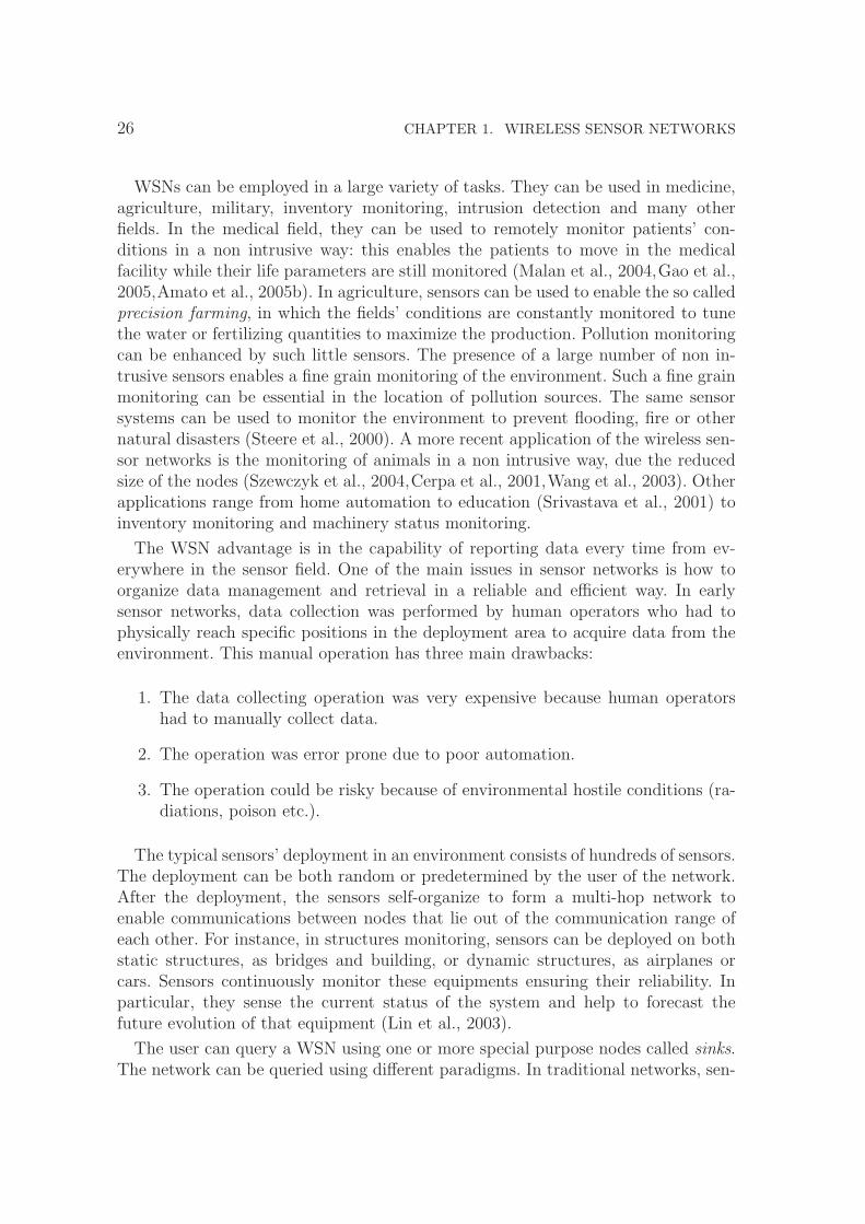
Wireless networks can be divided in two main categories: the infrastructured andthe ad hoc networks.
Infrastructured networks. Infrastructured networks have one or more central co-ordination points. A good example of such networks are cellular networks (Rahnema,1993). To communicate to another peer, each cellular device needs to negotiate withthe infrastructure hardware of the cell it belongs to. Once this communication hastook place the infrastructure takes care of setting up a channel between the peers(and to manage accounting, related services etc.). It seems a paradox, but all thecommunications in an infrastructured network must use the infrastructure. In cel-lular networks the communication between two peers must pass throughout thenetwork infrastructure also if the two devices could be able to communicate to eachother because they are in the transmission range of each other. As depicted in Fig-ure 1.1.a, two peers belonging to two different cells need to communicate to therespective cell manager to set up a communication. The same happens in the casedepicted in Figure 1.1.b, in which the two peers would be able to communicatedirectly but need to use the infrastructure.
Ad hoc networks. Ad hoc networks are totally self-organizing and usually do notrely upon any centralized authority. A distinguished feature of ad hoc networksis being able to organize themselves to perform any activity (e.g. routing, balanceddata storage, etc.) without a centralization point. All the peers of an ad hoc networkmust perform two different roles: (i) the role of an active communication peer (assender or receiver) and (ii) the role of passive communication peer, performing

28 CHAPTER 1. WIRELESS SENSOR NETWORKS
switchednetwork
(a) Communication between different cells (b) Communication in-side the same cell
Figure 1.1: Peers’ communications in infrastructured networks. (a) depicts the com-munication between two peers located into two different cells using the infrastructureto communicate and (b) two peers inside the same cell that need to uses the infras-tructure too.
routing for the other peers’ communications. In this sense, ad hoc networks arecollaborative networks in which all the nodes need all the others to be able to setup communications.
A particular kind of ad hoc networks is given by WSNs. WSNs (Akyildiz et al.,2002a) are formed by hundreds, or even thousands, of simple nodes that are deployedto monitor areas of interest. Each node is able to acquire data from the environment,store the sensed data, possibly after little processing, and coordinate to route theacquired data to one or more special nodes, namely the sink nodes. Usually the sinknodes store and use data in different ways depending on the user’s needs. Due totheir strict constraints in CPU performance, memory on board and battery lifetime,WSNs represent an “extreme” case of ad hoc networks because all the problemsrelated to ad hoc networks are amplified by such strict constraints.
1.1.2 Applications of wireless sensor networks
Due to the nature of self-organization, the WSNs have found a lot of applicationsin all the fields that need to collect data in environments in which a predefinedinfrastructure cannot be built up for different reasons: due to time and/or spaceconstraints, or more simply, the user does not want to build such infrastructure.
Military. Military applications are the simplest to imagine. WSNs can be set upto monitor the battlefield or to create intrusion detection systems. In a similar waywireless sensor networks can find an application in the monitoring of ammunition orto create an easily deployable communication infrastructure in which each soldier isequipped with a sensor. This sensor can be used to communicate with other soldiersand to monitor soldiers’ health status.

1.1. APPLICATIONS, TECHNOLOGY AND ARCHITECTURE 29
Medical. WSNs can be used also for medical purposes. We can think to employthem to monitor patients when they move inside the hospital or to locate medicalstuff, for instance a moving x-ray machine, inside the same structure.
Environmental. Another application is represented by environmental monitoringand control. In this scenario, sensors can be attached to objects, for instance indus-trial robots, to control their status and position and to send commands to them.In this way, we can also use sensors to locate some furniture or devices quickly, forinstance monitors or projectors, in an office.
Domotics. In domotics, WSNs can be used as the underlying architecture to provideall the features required by domotics applications. For instance, sensors can be usedinside rooms to monitor the presence of people to automatically turn on and offlights.
Assisted learning. In a possible assisted learning application, people are free tomove inside a museum and when they arrive close to an object of the museumcollection, an automatized system can start to describe the object. Moreover, thesensors can synchronize themselves with other sensors-like devices that visitors bringwith them to provide a multilingual description of the object.
Disasters. Finally WSNs can be used in disaster areas with two main applications:the first is to create an easily deployable communication system and the second oneis to monitor, in real time, the evolution of a dangerous environment.
1.1.3 Technology constraints of wireless sensor networks
In most applications, sensors have to be small and cheap. They need to be smallbecause during their usage they must be “invisible” (military surveillance) or becausepatients in a hospital cannot be expected to carry a workstation on their back to bemonitored. They also need to be cheap because in military or disaster monitoringsensors are dropped in areas where, probably, no one wants to enter. When a sensorbreaks down, or its battery is over, no one will repair it and the device is goneforever.
Due to their nature of small and cheap devices, sensors have very limited resources.Current sensors are equipped with a small battery, a CPU with very low computa-tional power (MICA-MOTEs from Crossbow Inc.∗ have an 8MHz processors with8 bits words), memory limited to few hundreds of kilobytes, a wireless communi-cator (radio or IR) and some acquisition devices (for temperature, pressure, etc.).Figure 1.2.a depicts the standard architecture for a sensor node. The architecture isvery simple and made up few components as said before. Figure 1.2.b depicts a realsensor. To give a scale factor for such devices its measures are 58×32×7 millimetersand it weights 18 grams (excluding batteries).
∗ www.xbow.com

30 CHAPTER 1. WIRELESS SENSOR NETWORKS
ProcessorMemory Radio
acquisit iondevice
acquisit iondevice
...
(a) Sensor architecture (b) A MICA-MOTE sensor node
Figure 1.2: Sensor node. (a) depicts the typical architecture of a sensor, made up ofa processor, memory, some acquisition devices and a radio. (b) depicts the photo ofa real sensor node.
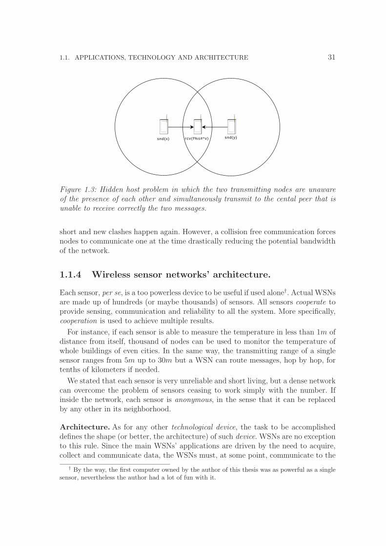
Like in other wireless networks, in WSNs, packet collisions due to multiple com-munication taking place in the same space at the same time is more difficult tohandle than in wired networks. In traditional wired networks, when an host sendsa packet, the host is able to receive its own signal on the on the same cable. In thisway, it is easy to notice interferences due to packet collisions. On the other hand,in wireless networks, we can experience the so called hidden terminal problem (orhidden host problem). As depicted in Figure 1.3, when two hosts (that are not incommunication range of each other) send a packet at the same time to a commonreceiver, it will receive only a junk transmission. However, none of the senders is ableto detect the collision without help. The hidden host problem is solved using MAClevel protocols which exchange a few control messages to rule out all the possiblecollisions before starting a real sending operation (Fullmer and Garcia-Luna-Aceves,1997).
A similar problem arises when a large number of devices try to communicate inthe same area. In this case, the communications collide frequently and the problemknown as channel contention may rise. In the channel contention problem manynodes share the same subarea and all the nodes are able to communicate each other.When two or more nodes try to communicate at the same time (also to differentreceivers) their requests to establish a communication clash and the nodes try againto send the requests. This problem has a domino effect on the sensor nodes: at thebeginning it limits bandwidth because packets need to be transmitted again and thenthe retransmissions’ cost is payed by the sensor via battery exhaustion. Again wecan use suitable MAC protocol strategies to orchestrate the channel access in orderto avoid collisions. Typical techniques used to avoid such clashes take care of waitinga random time before trying again to communicate. If the number of nodes trying tocommunicate is high the time range in which they randomize that time can be too
1.1. APPLICATIONS, TECHNOLOGY AND ARCHITECTURE 31
snd(x) snd(y)rcv( f%s#*v)
Figure 1.3: Hidden host problem in which the two transmitting nodes are unawareof the presence of each other and simultaneously transmit to the cental peer that isunable to receive correctly the two messages.
short and new clashes happen again. However, a collision free communication forcesnodes to communicate one at the time drastically reducing the potential bandwidthof the network.
1.1.4 Wireless sensor networks’ architecture.
Each sensor, per se, is a too powerless device to be useful if used alone†. Actual WSNsare made up of hundreds (or maybe thousands) of sensors. All sensors cooperate toprovide sensing, communication and reliability to all the system. More specifically,cooperation is used to achieve multiple results.
For instance, if each sensor is able to measure the temperature in less than 1m ofdistance from itself, thousand of nodes can be used to monitor the temperature ofwhole buildings of even cities. In the same way, the transmitting range of a singlesensor ranges from 5m up to 30m but a WSN can route messages, hop by hop, fortenths of kilometers if needed.
We stated that each sensor is very unreliable and short living, but a dense networkcan overcome the problem of sensors ceasing to work simply with the number. Ifinside the network, each sensor is anonymous, in the sense that it can be replacedby any other in its neighborhood.
Architecture. As for any other technological device, the task to be accomplisheddefines the shape (or better, the architecture) of such device. WSNs are no exceptionto this rule. Since the main WSNs’ applications are driven by the need to acquire,collect and communicate data, the WSNs must, at some point, communicate to the
† By the way, the first computer owned by the author of this thesis was as powerful as a singlesensor, nevertheless the author had a lot of fun with it.

32 CHAPTER 1. WIRELESS SENSOR NETWORKS
(a) WSN without sinks (b) WSN using a sink
Figure 1.4: WSNs architectures. (a) depicts a sensor network without a sink nodeand where each node is able to communicate to the user (in this case using a satelliteup-link). (b) depicts a sensor network with a sink node that collect the data from thesensors, via multi-hop communication, and then it sends data to the user using asatellite up-link.
external world the acquired data. This can happen in two ways: either every nodecan communicate to the user or only few nodes can do that.
In the first case (Figure 1.4.a), we can imagine that all sensors have enough powerto communicate out of the area of interest (e.g., using a satellite up-link) or, sometimes, the user can enter the area and use a sensor-like device, for instance attachedto a laptop, to query the devices.
In the second case (Figure 1.4.b), we have one or more special nodes, called sinks,that collect and communicate data to the user. Sink nodes are special nodes, differ-ent from other sensors, with more computational power and battery. They can bealways active, active only at pre-established times or active at request by the user.Sinks are gateways between the users of WSNs and the network itself. The kind ofinterconnection between the sink and the outside world is not part of the WSN andit can take place in a large number of forms.
Inside WSNs, the communications can take place in only two ways: single-hopand multi-hop. In single-hop communications, data are exchanged directly from thesender node to the receiver node. In multi-hop communications, one or more interme-diate nodes route communications between senders and receivers not in transmissionrange.

1.2. AN ABSTRACT WIRELESS SENSOR NETWORKS MODEL 33
Deployment. Roughly speaking, sensors can be deployed only in two ways‡: (i)“by hand” or (ii) randomly.
In the deployment “by hand”, sensors are placed one by one in specific locationsto create networks with desired characteristics, for instance sensors can be deployedto form a mesh or tori or, more simply, the sensors are placed to be aware of theirposition, of the position of the other sensors and of the position of the sink. Thisplacement can be used to easily set up communications, find routes and keep trackof the distribution and so on.
On the other hand, random deployment in the area of interest is performed withmuch less control. For instance, when sensors are dropped from an airplane or firedout from some fixed location, we could know the approximated distribution of thesensors in the sensing field but the exact position of each sensor (sometimes we arenot aware of the distribution too) is definitely unknown. This kind of deploymentgenerates a lot of problems: the nodes have to effectively self-organize to find outtheir relative positions and to find out the sink node(s) before the sensing operationscan take place.
As a kind of pervert version of the icing on the cake, sensors can move duringtheir lifetime. This usually happens by means of an external force, for instance ifthe sensors are dropped in a tornado to monitor air-flows or when a WSN, deployedto monitor a slope, starts to move with the mountains itself.
Apart from the “by hand” deployment, random WSNs deployment is a crucialpart of the WSNs’ architecture. The deployment introduces problems into a WSNconfiguration and performance. Partitioned WSNs can miss the connection to thesink, also for a large part of the nodes. Moreover, a non-uniform distribution of thenodes can bring to pathological states of unfair load distribution across the networkif not properly managed.
1.2 An abstract wireless sensor networks model
In this section, we present our reference model for wireless sensor networks. Themodel is used throughout this thesis to develop our studies. We also discuss someproblems and some simplifications with respect to the reality. The model that we aregoing to use is widely accepted and used by the scientific community (Bettstetter,2004a), (Santi et al., 2001), (Santi and Blough, 2002), (Xue and Kumar, 2004),(Panchapakesan and Manjunath, 2001), (Gupta and Kumar, 1998) and (Dousseet al., 2002).
In our abstract model, we represent the sensors as zero-dimensional points in Rd,with d ∈ {1, 2, 3}. Each sensor, si, can communicate with other sensors with its
‡ All the other, “picturesque”, ways in which sensors can be deployed by, fall in one of thesetwo categories.

34 CHAPTER 1. WIRELESS SENSOR NETWORKS
antenna. The communication range, r, can be fixed or can vary in some interval(0, rmax] for each one or all the sensors.
The communication range r, is a critical factor in wireless sensor networks becausethe energy consumption in data transmission is very large and grows as a super-linearfunction of the range. In our model, the power pi used by si to transmit correctlydata to sj must satisfy the following inequality
pi
δαi,j
≥ β, (1.2.1)
where α ≥ 2 is the distance power gradient, β ≥ 1 is the transmitting qualityand δi,j is the Euclidean distance between si and sj in Rd. Typically β = 1 andα depends from the environment in which the communication happens. In the idealcase α = 2, but in more realistic conditions α = 4 (α ∈ [2, 6]).
Equation (1.2.1) describes the energy used by the sender, but we must remember,that also the receiver uses energy to receive and to decode the signal and this factoris taken in account in our experiments.
Thus, a WSN can be represented as a graph in which vertices represent sensorsand edge exists between si and sj if and only if δi,j ≤ r. When the sensors aredeployed randomly in Rd, this structure is called Random Geometric Graph (RGGfor short (Bollobas, 1985)).
1.2.1 Missing features
The model previously presented is widely accepted by WSNs community as a rea-sonable approximation of the reality. However, communications in WSNs show someinteresting properties which are not captured by the model. Here, we give a briefoverview of these properties and we point out which part of the model should berefined to take them into account. The aim of this discussion is to make the readeraware of the approximations introduced.
A first, important, difference is that in the real world the communication volumethat the transmitting range draws around the sensor is not a perfect sphere. In thereality, we must consider a spheroid of radius r with a log-normal perturbation
LN(x) =
exp
[
−12
(
ln(x)−µσ
)2]
√2πσ2x2
(1.2.2)
Equation (1.2.2) highlights that the range r has a high probability to be lightly mod-ified, and a very low probability to be modified significantly. Figure 1.5 depicts thedifferences between a circular communication range and a log-normally perturbedcommunication range. In Figure 1.5.a the communication range is a perfect circle
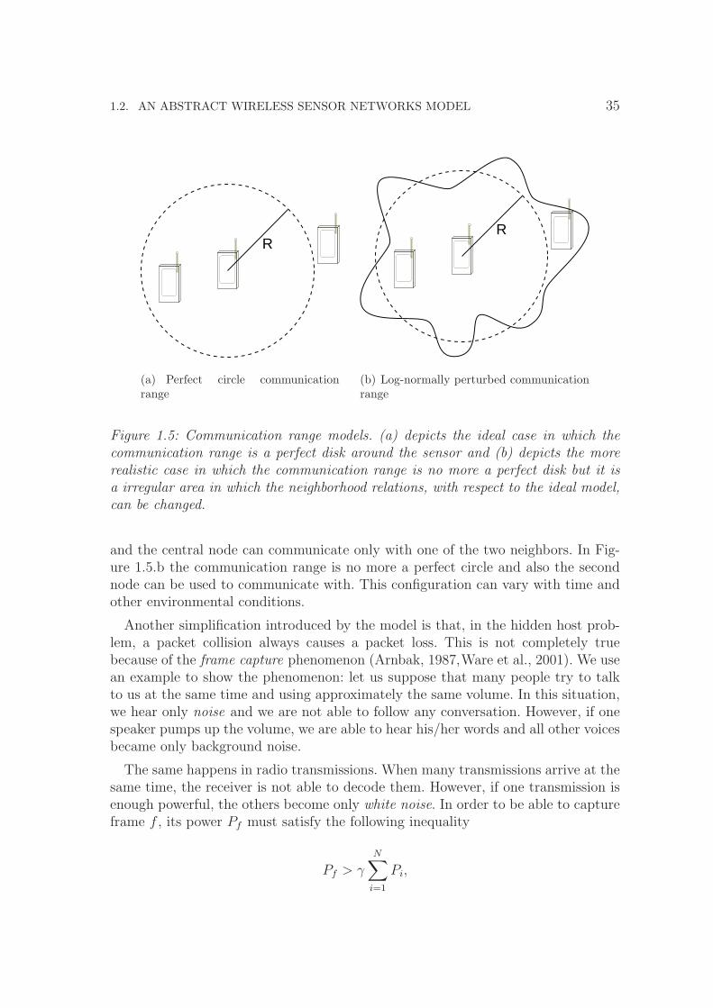
1.2. AN ABSTRACT WIRELESS SENSOR NETWORKS MODEL 35
R
(a) Perfect circle communicationrange
R
(b) Log-normally perturbed communicationrange
Figure 1.5: Communication range models. (a) depicts the ideal case in which thecommunication range is a perfect disk around the sensor and (b) depicts the morerealistic case in which the communication range is no more a perfect disk but it isa irregular area in which the neighborhood relations, with respect to the ideal model,can be changed.
and the central node can communicate only with one of the two neighbors. In Fig-ure 1.5.b the communication range is no more a perfect circle and also the secondnode can be used to communicate with. This configuration can vary with time andother environmental conditions.
Another simplification introduced by the model is that, in the hidden host prob-lem, a packet collision always causes a packet loss. This is not completely truebecause of the frame capture phenomenon (Arnbak, 1987,Ware et al., 2001). We usean example to show the phenomenon: let us suppose that many people try to talkto us at the same time and using approximately the same volume. In this situation,we hear only noise and we are not able to follow any conversation. However, if onespeaker pumps up the volume, we are able to hear his/her words and all other voicesbecame only background noise.
The same happens in radio transmissions. When many transmissions arrive at thesame time, the receiver is not able to decode them. However, if one transmission isenough powerful, the others become only white noise. In order to be able to captureframe f , its power Pf must satisfy the following inequality
Pf > γN
∑
i=1
Pi,
36 CHAPTER 1. WIRELESS SENSOR NETWORKS
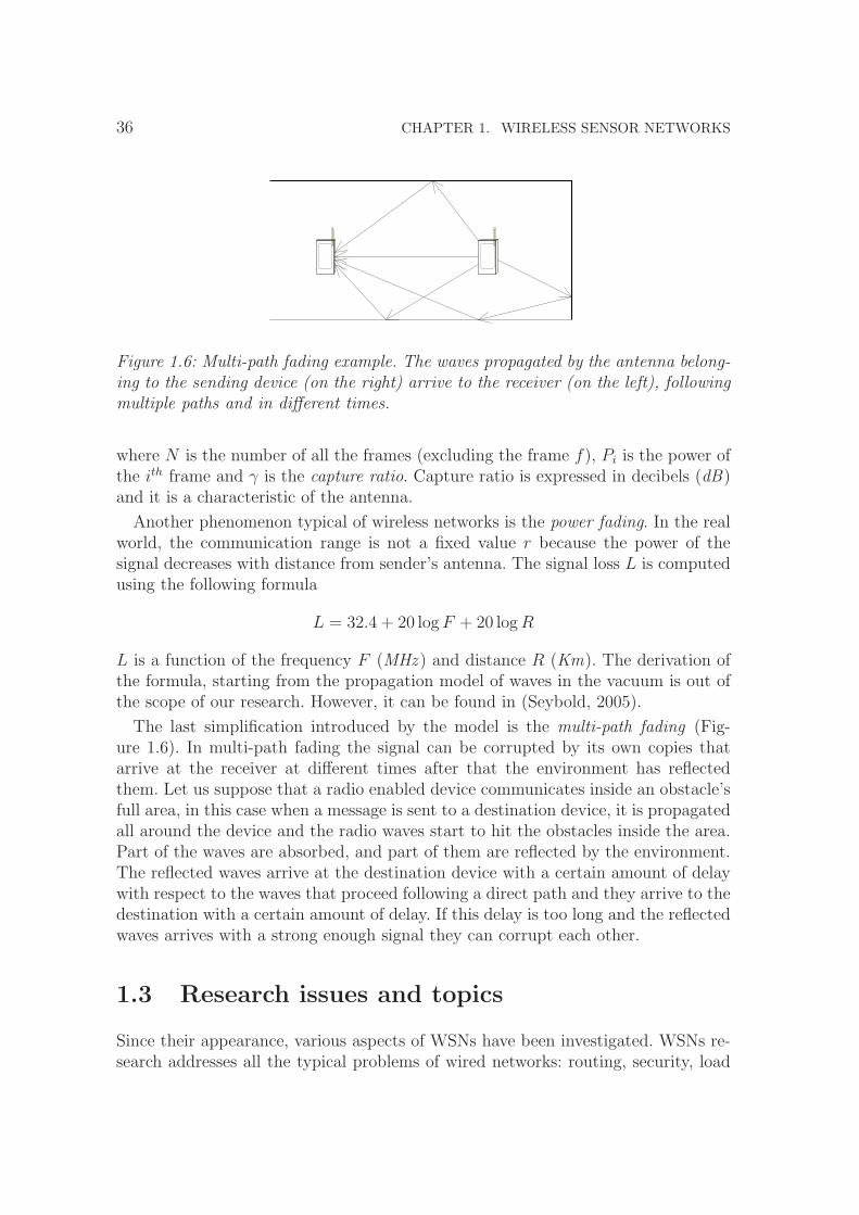
Figure 1.6: Multi-path fading example. The waves propagated by the antenna belong-ing to the sending device (on the right) arrive to the receiver (on the left), followingmultiple paths and in different times.
where N is the number of all the frames (excluding the frame f), Pi is the power ofthe ith frame and γ is the capture ratio. Capture ratio is expressed in decibels (dB)and it is a characteristic of the antenna.
Another phenomenon typical of wireless networks is the power fading. In the realworld, the communication range is not a fixed value r because the power of thesignal decreases with distance from sender’s antenna. The signal loss L is computedusing the following formula
L = 32.4 + 20 log F + 20 log R
L is a function of the frequency F (MHz ) and distance R (Km). The derivation ofthe formula, starting from the propagation model of waves in the vacuum is out ofthe scope of our research. However, it can be found in (Seybold, 2005).
The last simplification introduced by the model is the multi-path fading (Fig-ure 1.6). In multi-path fading the signal can be corrupted by its own copies thatarrive at the receiver at different times after that the environment has reflectedthem. Let us suppose that a radio enabled device communicates inside an obstacle’sfull area, in this case when a message is sent to a destination device, it is propagatedall around the device and the radio waves start to hit the obstacles inside the area.Part of the waves are absorbed, and part of them are reflected by the environment.The reflected waves arrive at the destination device with a certain amount of delaywith respect to the waves that proceed following a direct path and they arrive to thedestination with a certain amount of delay. If this delay is too long and the reflectedwaves arrives with a strong enough signal they can corrupt each other.
1.3 Research issues and topics
Since their appearance, various aspects of WSNs have been investigated. WSNs re-search addresses all the typical problems of wired networks: routing, security, load

1.3. RESEARCH ISSUES AND TOPICS 37
distribution and the like. Moreover, there are problems which are peculiar of WSNs.For instance topology control, in which the network structure is adjusted, settingcommunication ranges, to satisfy some requirement. However, any research in wire-less sensor networks must take in account some specific constraints:
Low energy, sensors are equipped with small batteries. Since computations andwireless communications have a high cost, algorithms and protocols shouldhave a low complexity and communications should be reduced as much aspossible.
Limited bandwidth, the transmission power must be kept low to save sensor en-ergy, therefore, only a few bytes of data can be exchanged in the time unit inorder to save energy.
Unstructured and varying topologies, sensor nodes can sleep to save power orthey can have faults or, more simply, they can move. In all the cases, as aresult, we have a topology change and, for instance, the routes from a sensorto the sink may change and they must be computed again, and/or some datumcan be lost.
Low-quality communications, low energy communications tend to be receivedwith a lot of errors at long distance and WSNs must be able to cope with itusing correcting codes and/or retransmissions.
Hostile environment, the nodes can be destroyed by the environment and/or envi-ronmental radiations can cause transmission failures. In any case the protocolsmust be tolerant to such events as in the case of topology changes.
In the rest of this thesis, we focus on non-uniformity, in its influence in WSNsand how we can overcome the problems that are originated by it. To show up thenon-uniformity influence and the techniques that can be used to get rid of it we usea case study. Our case study is the non-uniformity issues in data management inWSNs.
Research on data management. Data management research covers the problemsrelated to storing data in a balanced and fault-tolerant way in WSNs. The impor-tance of these problems is due to the unreliable nature of sensors and by the lowquantity of memory on board.
The central problem to be solved is to be able to locate data in an efficient wayfor both store and load operations. In WSNs, data can have two different ways tobe located. Some data are localized in some area and must be stored there, forinstance, the temperature measured in a given place can be kept in such a place.On the other hand, other kind of data are not related to a particular location, forinstance, the average temperature of a region has not a particular position in which

38 CHAPTER 1. WIRELESS SENSOR NETWORKS
it can be stored in. This last kind of data must be stored in a way such that: (i)it balances the load across the whole network and (ii) it is readily accessible whenneeded. Moreover, data produced at a high rate can easily fill the memory of a singlesensor and it must be stored around the network in a balanced way.
A promising approach to data storage in WSNs is based on geographic hash ta-bles (Ratnasamy et al., 2003). In this approach, a datum is identified by a key andthere is a hash function that provides, given the key, the geographical coordinateswhere the datum must be stored in or can be loaded from. The hash function is usedto distribute data in a balanced way, giving to each sensor the same amount of datato store. The protocol stores data in some sensors in the proximity of the coordinateidentified by the hash function, in this way it adds fault tolerance because data isstored in multiple nodes.
As we will point out in Chapter 4, the geographic hash tables, as they are presentedin (Ratnasamy et al., 2003), tend to have problems in presence of non-uniformityboth for the load distribution and for the fault tolerance aspects. For these reasons,we have chosen to use them to point out some of the typical problems introduced bynon-uniformity and to show up what is the path that we must follow to solve theseproblems.
1.4 Summary
In this chapter, we reviewed the principal features of WSNs, giving a gentle intro-duction to them. We reviewed the architectural properties of both single sensors andof the networks made up of these little devices.
WSNs are a special case of ad hoc networks: once deployed in an area of interest,the sensors have to self organize to provide the basic network services as routing. Themain difference between ad hoc networks and WSNs is given by the tight constraintsof such kind of networks.
While ad hoc networks are made up of devices, such as PDAs, whose compu-tational power increases everyday, WSNs are made up of inexpensive devices withlimited resources, both in terms of energy and computational power.
These constraints move all the ad hoc networks’ problems to a more difficultlevel of resolution: algorithms need to be simple and very fast, protocols need fewmessages to be executed and brand new energy saving strategies have to be foundto keep the network fully functional.
Then, we moved in the definition of an abstract model of WSNs useful for theanalysis and for the formalization of our research in the field of WSNs. Our model issuited to catch the problems that we are going to present in the next chapters. Weneed a suitable model to study the influence of non-uniformity in WSNs. For thisreason, we need to be free from all the characteristics that are not influenced (ornot influenced very much) by non-uniformity. In our research, we need to focus on

1.4. SUMMARY 39
the distinguishing characteristics of the non-uniformity issues that can influence, ina negative or positive way, the current results in WSNs that were build up on topof the uniformity assumption.
In the next chapter, we are going to give full suite of motivations to the reasons waythe uniformity dogma is not suitable for WSNs’ research, how we can characterizenon-uniformity and how we can start to think in a non-uniform way to create non-uniformity aware architectures, protocols and systems.

40 CHAPTER 1. WIRELESS SENSOR NETWORKS

Chapter 2
Non-Uniformity
Variety of mere nothings gives more pleasure than uniformity of something.- Jean Paul (Johann Paul Friedrich Richter)
Abstract
Most of current WSNs research focus on uniform networks: networks in whichsensors are equals to each other or networks that are distributed followingthe uniform distribution. In current WSNs research, uniformity is a dogma, abelieved true assumption that no one wants to offend. In this chapter, we startfrom a slightly different point: we simply state that uniformity does not exist.Moreover, the uniformity assumption that can be found in the mainstreamWSNs research produces solutions that can be non-tolerant with respect tonon-uniformity and these solutions can be difficult to adapt to a non-uniformenvironment. In this chapter, starting from the consideration that uniformitydoes not exist, we begin to study non-uniformity and its influence in WSNsresearch.
In this chapter, we introduce non-uniformity and its influence in WSNs. Our in-tention is to show that the typical uniformity assumption found in almost all theresearch work in WSNs field is best suitable to be defined as an uniformity dogma:the assumption was never motivated by anyone, but was assumed as something trueand reasonable.
In this chapter, we start with some general consideration about the uniformitywhich target is to disrupt the uniformity dogma: we show how the uniformity israrely present in nature and, as a consequence of this, in every human artifact asWSNs.
Once this task is performed, we review non-uniformity: we describe it formallyand we present four models of non-uniformity that may influence WSNs, namely
42 CHAPTER 2. NON-UNIFORMITY
the deployment non-uniformity, the geographical non-uniformity, the functional non-uniformity and finally the movement non-uniformity.
These models present a rough taxonomy of non-uniformity and we do not pretendthat this taxonomy is the best one or the only one: we define this taxonomy becauseit is an aurea mediocritas for the model developed in the rest of the thesis and areasonable representation of the main characteristics of non-uniformity for WSNs.
Chapter organization. This chapter is organized as follows. Section 2.1 points outthe importance of the non-uniformity as a substantial part of WSNs research. Sec-tion 2.2 presents our taxonomy of the non-uniformity in WSNs. Section 2.3 presentsthe (few) related work on non-uniformity in WSNs. Finally, Section 2.4 draws theconclusions of the work described in this chapter.
2.1 Why does non-uniformity matter?
In our opinion, non-uniformity matters because in “nature” perfect uniformity doesnot exist.
If we observe reality from a distant point of view, we can find uniformity almosteverywhere. However, if we pay more attention in observing the world, for instancewith a magnifying lens, we are no more able to find such uniformity.
As a common experience, if we observe the smooth marble surface of a beautifulrenaissance statue we can argue that it is uniform: no asperities can be perceived byeyes or fingers. But, if we observe it using a microscope, this uniformity gets lost:the unveiled surface is full of asperities and it does not look possible that it couldbe the same surface as before.
In computer science, sometimes we manage data structures or algorithms thatneed to be uniform. For instance, when we use hash tables we need to provideuniform hashing algorithms to have a good distribution of data and in turn of thisprovide balanced tables. Moreover, in randomized and Monte-Carlo algorithms, weneed uniform random number generators to explore in a random, but fair, waysome result space. But, when we want to simulate, or analyze the real world, wecannot pretend that the simulated world behaves uniformly because in the realworld uniformity is far from reality.
This happens in WSNs research too. Even if we distribute sensors “by hand”and we create structures with interesting properties as grids, meshes and so on,we cannot call them uniform because we may introduce some errors during thedistribution and/or once distributed it may happen that their behavior (for instancethe transmitting range) is not uniform.
If we drop sensors from above, using an airplane or a helicopter, we cannot obtainan uniform distribution at all. The sensors are more likely to fall accordingly to somemore complex distribution such as Gaussian or Gaussian-like distributions.

2.2. MODELS OF NON-UNIFORMITY 43
Now, let us suppose that we can distribute sensors with perfect uniformity. Prob-ably the environment itself is not uniform. Real applications of sensors include bat-tlefields, harsh regions and urban scenarios. Scenarios too variegated and complexto be defined as uniform (or to find some kind of ruled non-uniformity as a Gaus-sian curve): these scenarios have obstacles that, for instance, change the behavior oftransmissions, disabling the sensors to communicate each other.
2.2 Models of non-uniformity
In this section, we present the four models of non-uniformity that we have spottedout during the development of this thesis. The classification of the models of non-uniformity, that we developed, is a suitable high-level classification that catches thefour main families of non uniformity. We do not think that this classification is theonly possible one. As stated before in this chapter, these four families representsan aurea mediocritas, literally a golden way in the middle: this taxonomy catchesthe essential differences between the different kinds of non-uniformity and it definesonly four models but it may be extended in multiple ways mixing up two, or more,of the presented models or creating sub models inside the ones presented here.
In a WSN, we can find different kinds of non-uniformity, appearing in differentsituations. Non-uniformity can be due to the method used for the deployment ofthe network (e.g., when the sensors are dropped from above) or it can depend onsome functional patterns of the WSN itself. Moreover, non-uniformity can be due tothe geography or by obstacles present in the deployment area. Finally, a last kindof non-uniformity is typical of WSNs in which the nodes can move, by themselvesor simple because the environment can move.
We refer to these four models as: the deployment non-uniformity, the geograph-ical non-uniformity, the functional non-uniformity and finally the movement non-uniformity.
Intentional AccidentalStatic Deployment Geographic
Dynamic Functional Movement
Table 2.1: Our taxonomy of non-uniformity in WSNs.
We developed this taxonomy for the models of non-uniformity because, in ouropinion, this is a reasonable high level representation of the possible kinds of non-uniformity. Moreover, our taxonomy catches four aspects of the possible distribu-tions. Table 2.1 shows the four aspects. These aspects represent four main charac-teristics of distributions:
Intentional: the distribution that we are going to analyze (or its approximation)is known a priori. For instance, when we drop sensors from above, we are
44 CHAPTER 2. NON-UNIFORMITY
quite confident of the fact that they will distribute following a Gaussian-likedistribution.
Accidental: the distribution that we are going to analyze (or even its approxi-mation) cannot be known a priori. For instance, when we drop sensors on aterrain full of hills and depressions, we cannot estimate what the distributionwill be.
Static: the distribution that we have at the beginning will be almost the sameduring all the network lifetime. For instance, once we deploy the sensors, ifthe sensors cannot move, they will be in the same place for all the network lifetime.
Dynamic: the distribution of the sensors changes with time. If the sensors movesthe physical distribution changes. If the network is made up of different kindof sensors, its behavior changes with the possible interactions between nodes,considering that this behavior is known only at the network run time it has tobe considered dynamic.
2.2.1 Deployment non-uniformity
The way in which the sensors are deployed is the first cause of non-uniformity in ourtaxonomy. WSNs deployed by hand can be structured in very fascinating topologieswith a lot of interesting properties, such as meshes, tori and many more structureddistributed topologies. Unfortunately, real WSNs are usually deployed in a randomfashion.
Random WSNs deployment follows two main kinds of non-uniform distributions:Gaussian and skewed (Zhou et al., 2005).
The Gaussian distribution, depicted in Figure 2.1.a appears when the WSNs aredeployed from above, for instance when the sensors are dropped from an airplane orfrom any other kind of flying object. This kind of nodes distribution is well suitedfor military applications in which the sensors are deployed on the battlefield withoutany predefined pattern. The Gaussian distribution of sensors on a plane is describedby the following Equation
f(x, y) =1
2πσxσy
e−[((x−µx)2/2σ2x )+((y−µy)2/2σ2
y )]. (2.2.1)
Equation (2.2.1) is the result of the product of two independent Gaussian distri-butions. The terms µx and σx represent the mean and the standard deviation for theGaussian distribution on the x-axis; in the same way µy and σy represent the meanand the standard deviation of the distribution on the y-axis.
Typically Equation (2.2.1) is found in the form where both µx and µy at zero, torepresent the fact that the distribution is centered in an ideal (0, 0) point.
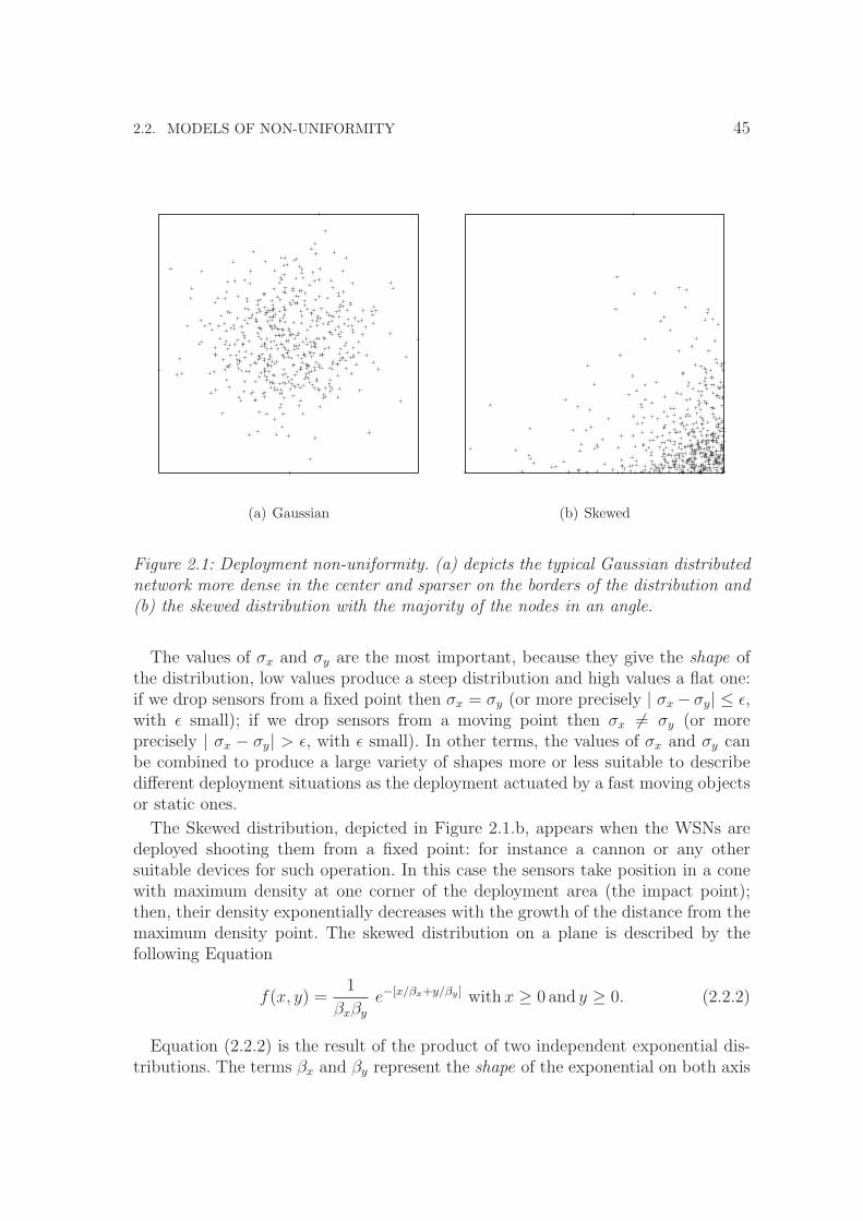
2.2. MODELS OF NON-UNIFORMITY 45
(a) Gaussian (b) Skewed
Figure 2.1: Deployment non-uniformity. (a) depicts the typical Gaussian distributednetwork more dense in the center and sparser on the borders of the distribution and(b) the skewed distribution with the majority of the nodes in an angle.
The values of σx and σy are the most important, because they give the shape ofthe distribution, low values produce a steep distribution and high values a flat one:if we drop sensors from a fixed point then σx = σy (or more precisely | σx − σy| ≤ ǫ,with ǫ small); if we drop sensors from a moving point then σx 6= σy (or moreprecisely | σx − σy| > ǫ, with ǫ small). In other terms, the values of σx and σy canbe combined to produce a large variety of shapes more or less suitable to describedifferent deployment situations as the deployment actuated by a fast moving objectsor static ones.
The Skewed distribution, depicted in Figure 2.1.b, appears when the WSNs aredeployed shooting them from a fixed point: for instance a cannon or any othersuitable devices for such operation. In this case the sensors take position in a conewith maximum density at one corner of the deployment area (the impact point);then, their density exponentially decreases with the growth of the distance from themaximum density point. The skewed distribution on a plane is described by thefollowing Equation
f(x, y) =1
βxβy
e−[x/βx+y/βy ] with x ≥ 0 and y ≥ 0. (2.2.2)
Equation (2.2.2) is the result of the product of two independent exponential dis-tributions. The terms βx and βy represent the shape of the exponential on both axis
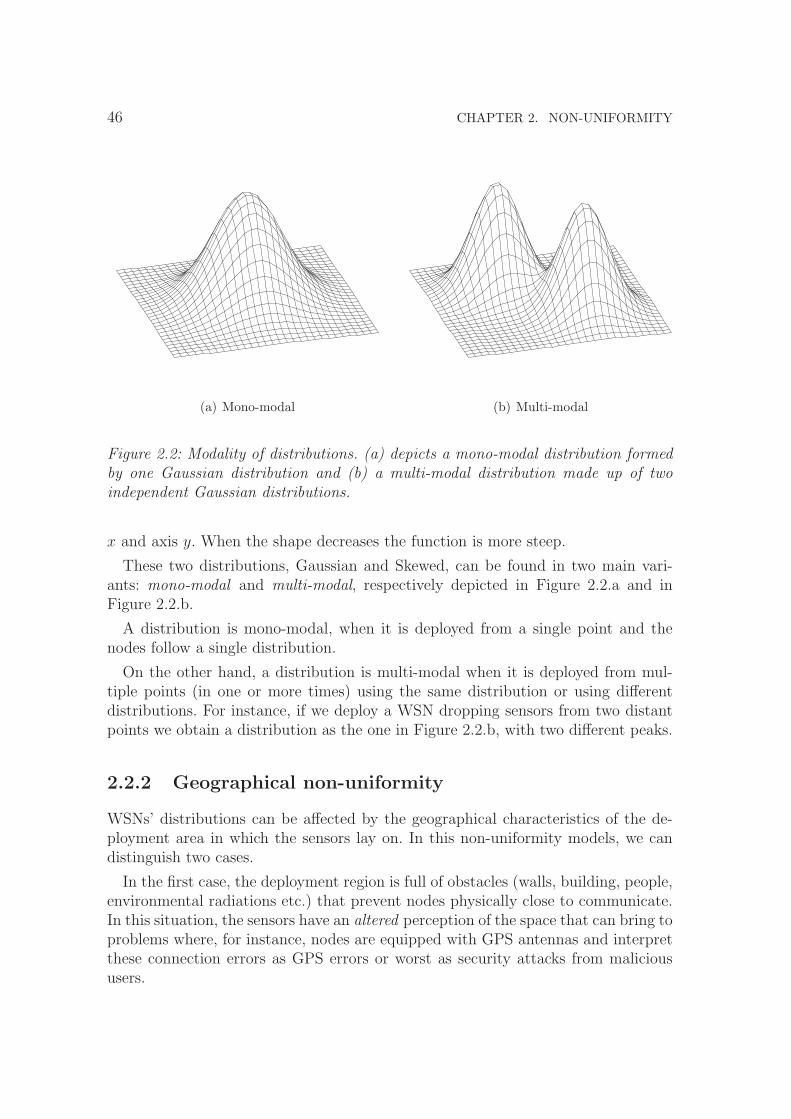
46 CHAPTER 2. NON-UNIFORMITY
(a) Mono-modal (b) Multi-modal
Figure 2.2: Modality of distributions. (a) depicts a mono-modal distribution formedby one Gaussian distribution and (b) a multi-modal distribution made up of twoindependent Gaussian distributions.
x and axis y. When the shape decreases the function is more steep.
These two distributions, Gaussian and Skewed, can be found in two main vari-ants: mono-modal and multi-modal, respectively depicted in Figure 2.2.a and inFigure 2.2.b.
A distribution is mono-modal, when it is deployed from a single point and thenodes follow a single distribution.
On the other hand, a distribution is multi-modal when it is deployed from mul-tiple points (in one or more times) using the same distribution or using differentdistributions. For instance, if we deploy a WSN dropping sensors from two distantpoints we obtain a distribution as the one in Figure 2.2.b, with two different peaks.
2.2.2 Geographical non-uniformity
WSNs’ distributions can be affected by the geographical characteristics of the de-ployment area in which the sensors lay on. In this non-uniformity models, we candistinguish two cases.
In the first case, the deployment region is full of obstacles (walls, building, people,environmental radiations etc.) that prevent nodes physically close to communicate.In this situation, the sensors have an altered perception of the space that can bring toproblems where, for instance, nodes are equipped with GPS antennas and interpretthese connection errors as GPS errors or worst as security attacks from malicioususers.

2.2. MODELS OF NON-UNIFORMITY 47
(a) Soil (b) Hill
Figure 2.3: Geographical non-uniformity. (a) depicts a sample geographic terrainconformation with a central valley and (b) an example of a network deployed accord-ingly to a Hill distribution with the sensors more dense in an angle.
In the second case, sensors dropped on a terrain tend to follow the terrain shapeand to fall into soil depressions. This situation can bring to networks in which thenodes are more dense in the valleys and less dense at high points. If we add the factthat hills can represents obstacles that prevent the sensor-to-sensor communications,we can have an highly partitioned network.
For the case in which sensors follow the terrain shape, we explore two differentdistributions. The first one, fully generic and related only to the geography, and thesecond one, that is a distribution function that approximates reality.
In the first one, as stated before, the terrain geography can cause node redistri-bution as depicted in Figure 2.3.a. The nodes deployed on steep terrains tend to falldown following the direction of the slope. This effect is per se complex to examineand to evaluate but it can become very difficult to model if we use it in conjunctionwith the effects of the deployment non-uniformity.
The second one is a distribution function that approximates reality. The Hilldistribution, depicted in Figure 2.3.b was first presented in (Orecchia et al., 2004a).The Hill distribution is very simple, and comes from an intuition and not fromexperimental results. This distribution simulates an uniform sensor distribution ona hill and the consequent fall of the sensors from the top of the hill to its base. Inthe paper, the authors provide only generator functions for the sensors coordinatesgeneration: x =
√u and y =
√v where u and v are uniformly distributed variables
in [0, 1]. From the generators, it is simple to find out the distribution function of thesensors on the plane
f(x, y) = 4xy with x ∈ [0, 1] and y ∈ [0, 1] (2.2.3)

48 CHAPTER 2. NON-UNIFORMITY
Equation (2.2.3) is very simple but reasonable and, at first sight, we can spot sim-ilarities with the Skewed distribution due to the maximum concentration in onecorner of the distribution.
2.2.3 Functional non-uniformity
The functional non-uniformity is related to functional patterns of the network itself.A single network can be made up by multiple kinds of sensors, with different ca-pabilities and constraints, or can be formed by a single kind of nodes behaving indifferent ways. These functional patterns are related to two basic concepts.
In the first one, the nodes of a WSN can adopt some kind of sleeping patternto enlarge life time as in (Ye et al., 2002), (Ye et al., 2004), (Cerpa and Estrin,2002), (Chen et al., 2002) and (Xu et al., 2001). The effect of these sleeping patternsis to create an effect of dynamic non-uniformity in which the sensors’ distributionis not only a function of the deployment method but also a function of time, thesensor “disappears” for some time and than “appears” again. Depending on thesleeping pattern, we can experience an effect of the same region that is alternativelymonitored by two or more networks sharing only few nodes.
In the second one, a single WSN can be made up of different kind of nodes withdifferent capabilities and constraints. An example of this kind of networks in whichtwo kind of nodes are present:
1. Sensing nodes, which are small and with low power, and perform data acqui-sition from the environment;
2. Communication nodes, which are more powerful and with a high power com-munication system, that can communicate at a larger distance providing abridge-like service between sub-areas of the network.
In this way, the sensing nodes can chose two ways to communicate: if they wantto communicate with close peers, they use the usual multi-hop communication butif they need to communicate with nodes that are far away, they can use the commu-nication nodes as communication highways. To have a perfect collaboration, that isa situation in which the two kinds of nodes works together to perform a monitoringtask, we require a load balancing between the sensing and communication nodesbecause in this case all communication nodes need to manage the same number ofsensing nodes.
One example of functional non-uniformity is provided by networks using threelayers of nodes: the sensing nodes, the sink nodes and the proxy nodes (Desnoyerset al., 2005). in this kind of networks, the proxy nodes collect data from the sensors,do some computation on these data and finally send data to sink nodes.
Another example is provided by Mules (Shah et al., 2003). The mules are movingproxies that go around the network collecting data from sensors and bring data toone or more sink nodes.

2.3. RELATED WORK 49
2.2.4 Movement non-uniformity
The last non-uniformity model that we want to present is the movement non-uniformity. This non-uniformity model can be due to two different factors. In thefirst one, the sensors are free to move in an autonomous and predictable way, for in-stance, the sensors that are piggybacked on moving objects such as industrial robotsthat the sensors are intended to monitor and control. In the second one, the sensorsare supposed to be stable and/or the movement is not predictable, for instance, thesensors are dropped in the water to track the flows or sensors that are attached toanimals and are used to monitor the wildlife.
The sensors distributions that describe movement non-uniformity are functionsof both time and space. Moreover, we can have situations in which the sensors canconverge to a single point and create a unbalanced network for a short period oftime, or the sensors can move randomly changing network topology continuously.
In literature we find few studies aimed to find out the characteristic distributionsfor movement uniformity. One of these, few, works is (Bettstetter, 2001). In thepaper, we can find a relevant study of this phenomenon limited to nodes that moveaccordingly to the random waypoint strategy (Johnson and Maltz, 1996). Thesesensors tend to create a node distribution (in function of the time) similar to aGaussian distribution. In random waypoint strategy, at the beginning each nodeis stationary in a random location, then it randomizes a point in the plane andmoves there, waits a random time and than moves again. This movement creates aconcentration of nodes in the middle of the area, because the nodes, to go from onepoint to another, cross the center of the area or pass nearby the center of the area.
2.3 Related work
Due do its nature of dogma, the uniformity assumption prevails in almost all theresearch work on WSNs. As a consequence of this, the study of non-uniformity inWSNs is an emerging topic. By now, only a few papers approach different problemsin WSNs taking into account networks deployed in a non-uniform way (Bettstetter,2004b), (Orecchia et al., 2004a), (Tilak et al., 2003), (Zhou et al., 2005) and (Bashet al., 2004). Between them, we can find non-uniformity depicted in two ways.
The first way addresses WSNs that are deployed in non-uniform fashion. In thisarea, we can find two main contributions. The first one is (Bettstetter, 2004b), inwhich the author studies the connectivity properties of sensor networks with uni-form and Gaussian distributions. For Gaussian distributions, given the transmittingrange of sensors and the shape of the distribution function, the author finds outthe radius around the maximum of the function in which all sensors are connected.A second result is (Orecchia et al., 2004a), in which the authors study the prob-lem of broadcast in sensor networks distributed with both uniform distribution and“Hill” distribution, which is a quite simple but reasonable distribution that we will

50 CHAPTER 2. NON-UNIFORMITY
study and use in the rest of the thesis. Finally, in (Zhou et al., 2005), the authorspropose a construction scheme of small worlds for the physical topology of Multiple-Input Multiple-Output (MIMO) wireless networks. In this work, the authors takeinto account various topologies (uniform, Gaussian, skewed and grid) to study thepossibility to create short cut channels to optimize the network communications.
The second way does not use non-uniformity in terms of deployment. In (Tilaket al., 2003) the non-uniformity is related to the concept of non-uniform informationgranularity. The non-uniform information granularity is related to the concept ofaccuracy of information. The paper states that the required accuracy, or precision, ofinformation is proportional to the distance between the producer and the consumerof the information. Another result is (Bash et al., 2004), in which the non-uniformityis related to information sampling from the network itself. The authors provide amethod to perform data sampling from a sensor network with approximately uniformmethods. Even when a network is non-uniformly distributed (they study the casein which the nodes are hand distributed into a building to monitor it), the authorspick data form the network uniformly. This is possible because the sensors spaceis normalized to an uniform space using Voronoi regions computed in a distributedfashion.
2.4 Summary
In this section, we introduced non-uniformity and we present some keys to motivateour work.
At the beginning, we presented the need for non-uniformity in current WSNsresearch and we pointed out how the uniformity dogma is widely used in researchwhile the world itself, that we are going to explore with our research, is, by its ownnature, non-uniform.
Then, we moved to the classification of various models of non-uniformity. Themodel that we propose out are general and each of them covers a large part ofpossible problems and networks. Our taxonomy of the models of non-uniformityis, intentionally, coarse gained. We preferred to give an intuitive division of thepossible sources of non-uniformity without being too formal. We know well that ourtaxonomy can be rewritten in a finer, or simply different, way but we think that afiner grain in the taxonomy does not help the comprehension of the problem itselfand it risks to be a pure formalization and style exercise.
Our classification presents four possible sources of non-uniformity. The deploymentnon-uniformity is related to the way in which the sensors are deployed in the interestarea by the user. The geographical non-uniformity is based on the idea that theenvironment that the sensors are intended to monitor influences the way in whichthe sensors can communicate. The functional non-uniformity catch the differentbehaviors of the sensors. Finally, the movement non-uniformity is related to theidea of movement of the sensors themselves.

2.4. SUMMARY 51
In the related work section, we presented the few papers that walked inside thenon-uniformity world and we realized that with the help of these few papers alone,we are not able to comprehend non-uniformity. Moreover, with the only help of thesepapers, we are not able to provide new solutions and, from our point of view moreimportant, a new way of thinking solutions that are able to deal with non-uniformity.

52 CHAPTER 2. NON-UNIFORMITY

Chapter 3
Data Management
“Data! Data! Data!” he cried impatiently. “I can’t make bricks without clay.”- found in “The Adventures of Sherlock Holmes”
Abstract
All the possible uses of WSNs deal with the idea of data acquisition and data
retrieval. These two concepts are strictly related because data retrieval is theresponse to a user query. The user should be able to actively program thenetwork, via control programs, to retrieve data that is considered useful. Intraditional WSN systems, these tasks consist in transmitting sensed data to apowerful node (the sink) which performs data analysis and storage. However,these models resulted unsuitable to keep the pace with technological advanceswhich granted to WSNs significant (although still limited) processing and stor-age capabilities. For this reason, more recent paradigms for WSN introduceddata base approaches to define the tasks of data sampling and processing, andthe concept of data-centric storage for efficient data access. In this chapter,we revise the main research contributions in the data management field.
All the possible uses of wireless sensor networks deal with the idea of data acquisition(by the sensors) and data retrieval (by the user). These two concepts are strictlyrelated because data retrieval is the response to a user query. The user should beable to actively program the network, via control programs, to retrieve data that isconsidered useful. This can be achieved in many ways, following various paradigms.
WSNs applications can be classified in two different families.
The first family is the one in which sensors continuously check the environment forsome particular data pattern (as in an intrusion detection system). In these applica-tions, the cooperation of nodes is be essential in providing extra information to theend user. Nodes that are aware of their own position can communicate to produce a
54 CHAPTER 3. DATA MANAGEMENT
localization of the event using triangulation or other systems (Bejar et al., 2001,Kr-ishnamachari et al., 2002). This collaboration is essential to provide meaningful datato the end user.
The second family is the one in which sensors are employed to monitor somephysical characteristic of the environment. For instance, sensors can provide thesensed temperature to the user. This use of the network produces data streamsfrom a single sensor to the sink. In this case, the real challenge in network datamanagement is to find an optimal strategy to delivery this (maybe) large amount ofdata to the user, in the most efficient way. The simplest approach to this problemis data aggregation. In data aggregation, the nodes used to perform routing (alsocalled relay nodes) take packets that are sent to the sink and combine the differentpieces of information in a single packet to reduce the total amount of transmissions.Data aggregation still works with small amount of data because the maximum sizeof packets is fixed and cannot be exceeded.
Modern approaches move the computation of data in the network itself (Maddenet al., 2002b, Madden et al., 2002a). Sensed data are not directly sent to the sinkand the computation is not done off-line: sensors that acquire data also processthem to extract information. The nodes can actively cooperate to produce highlymeaningful correlated data (such as the average, the variance and other statisticalmeasures or spacial and temporal associations of data). Moreover, these modernapproaches place the storage itself inside the network. In cases in which the sinkcan be unavailable for long periods of time (or in cases in which the sink is notpresent inside the network and the user has to enter the network to query it) theseapproaches are able to distribute data inside the network in such a way that thestorage is fault tolerant and load balanced. Some of these systems provide to theuser a high level distributed query language and engine (a la SQL) to query thenetwork.
Chapter organization. This chapter is organized as follows. Section 3.1 providesa brief introduction to the data management issues and models. Section 3.2 pointsout which services have to be provided by a data management system in WSNs andtheir underlying needs (e.g. routing). Section 3.3 describes the state of the art of thedatabase implementation inside WSNs. Section 3.4 gives a wide range introductionto the data centric storage (DCS) model, that will be the central topic of the researchwork that we present in Chapter 4. Finally, section 3.5 summarizes and draws someconclusions regarding the research work described in this chapter.
3.1 Data management in wireless sensor networks
In current WSNs, data management tasks are performed accordingly to differentnetwork storage models. A network storage model defines how to manage data insidea WSN, starting from data acquisition up to data retrieval by the user. For this

3.1. DATA MANAGEMENT IN WIRELESS SENSOR NETWORKS 55
reason, each network storage model needs to define how to implement, even partially,the basic services necessary to the good work of a data management system: (i)network programming, in which the sensors are programmed to replay to queries (setup of routes, data aggregation strategies etc.). (ii) data acquisition and in-networkaggregation, in which the data is physically acquired by transceivers and refined toproduce more useful streams. (iii) data retrieval, that provides the collection of databy an external entity.
In the literature, we can identify four main models to data management: namelyexternal storage, directed diffusion, data centric storage, and database model. Eachone of these models implements a part or all the above services. The services providedby these models are summarized in Table 3.1.
ExternalStorage
DirectedDiffusion
DataCentricStorage
DatabaseModel
Network programming no yes no yesData acquisition andin-network processing
partially partially yes yes
Data retrieval yes yes yes no
Table 3.1: Correspondence between models and services.
External storage is the simplest storage model and provides node cooperation onlyby data aggregation and data forwarding. Directed diffusion is able to program thenetwork to optimize the data flow from the sensors to the sink, providing a betterusage of the resources with respect to external storage. Data centric storage is ableto use the network to easily store and retrieve a datum using its meta-datum (anunique name for the datum) as a key. Data centric storage does not need, or provide,network programming facilities for the data management. Such facility can be addedon an upper layer laying on this one. Finally, the database model is able to abstractthe network as a relational database to perform complex queries that are executedby the sensors themselves.
In the rest of this section, we give more details on these four models. We will focusmore on directed diffusion and external storage because the data centric storage andthe database model will be the focus of the rest of this Chapter.
External storage model. In the External Storage (ES) model, the nodes send thesensed data, in both raw or more refined forms, to one or more sinks which performthe actual aggregation, processing and storage. In this model, the sensor nodesperform only data acquisition and send sensed data to the sink. To this purpose,they also have some routing capability. Each sink node collects data from the sensorsand implements an interface for the user. For instance, a sink might be a PC actingas router between the sensor network and other networks.

56 CHAPTER 3. DATA MANAGEMENT
The main advantage of this model is that it is simple to implement. Moreover, ifthe network produces few data it can be energy efficient.
The drawbacks of ES are represented by the poor usage of the network’s computa-tional resources because the sensors, that can be capable of more complex operationcould refine data. Moreover, data correlation is due to the sink and off line pro-cessing can require multiple sink-to-sensors communications while in an in-networkcomputation the sensors can efficiently self organize to provide correlated data. Forinstance, a user who wants to correlate various temperature sampling from a region(far from the sink) needs to query all the nodes of that region while an in-networkprocessing strategy is able to program the sensors of the same region to communicateand provide only the correlated data.
Diffusion model. Directed Diffusion (DD) is one of the first approaches proposedfor data management in sensor networks (Intanagonwiwat et al., 2000). The userrequests some specific data with a query including a tuple 〈key, value〉 and a datarate, which specifies the amount of data that must flow in the unit of time.
(a) interest dissemination (b) gradients (c) delivery of a datum
Figure 3.1: Directed Diffusion: (a) the interest dissemination from the sink node (ingray) to the sensor nodes (in white), (b) the gradients that are built in response tothe interest dissemination and (c) the delivery of data from a sensor node to thesink following one gradient.
The first step in data retrieval is represented by the interest dissemination phasein which the sink broadcasts the query in the network (as depicted in Figure 3.1.a).The broadcast used to disseminate the query sets up a directed acyclic graph (DAG)in the network which is rooted at the sink (as depicted in Figure 3.1.b). A node x isconnected to a set of upstream nodes (the gradients) which are its relay nodes whenx sends packets to the sink. Each node receives the query, records the query data rateand sets up the corresponding gradient toward the sink. The nodes that receive orsense some data that match one or more interests forward them up the route createdby the gradients according to the data rate (as depicted in Figure 3.1.c). The sink,at the reception of messages with the queried data, can exploit reinforcement of thepaths that bring data with higher data rates sending a packet down to the datastream. Reinforced paths may augment their data rate, while paths that are notreinforced expire after a given amount of time.

3.1. DATA MANAGEMENT IN WIRELESS SENSOR NETWORKS 57
The main advantage of the DD model is that the interest propagation happenshop by hop and the network does not need to use long communications to set up ormodify paths’ characteristics. DD is able to provide multi-path routing and deliveryusing the reinforcement of multiple paths. The nodes are capable to repair or tunethe paths in a local way sending local reinforcement messages.
DD presents also two main drawbacks. The first one is related to the poor loaddistribution of the protocol: the nodes that are closer to the sink are burdenedwith data and control packets. The second drawback is the limited opportunityfor in-network data processing because data may pass through different paths andaggregation and processing often happens only at the sink or at its neighbors.
Some recent improvements on DD have been proposed in (Marcucci et al., 2005)and (Liu et al., 2003,Liu et al., 2005).
In (Marcucci et al., 2005), the authors present Directed Diffusion Light (DDL).The improvement of DDL acts on interest propagation: each node can have only alimited set of gradients (while in DD the size of this set was not limited). In thisway, the DAG is sparser and it is not formed by all the nodes in the network. Whenreinforcement is performed the DAG may change to include previously discardednodes. This offers the opportunity of replacing depleted nodes with fresh spares andthus extends the network lifetime.
Figure 3.2: Information Directed Routing: a message from the query proxy node tothe exit node, does not follow the shortest path (the dashed line), but follows a longerpath (solid line) to get data from the nodes inside the dark gray area.
In (Liu et al., 2003,Liu et al., 2005), the authors present the Information DirectedRouting (IDR). IDR can operate in two ways. In the first way, a source node injectsa query with a particular interest and such query is routed throughout a path buildupon interest gradients spread by the possible query receivers. In the second way,depicted in Figure 3.2, it is able to find paths between a source node and a destinationnode (called respectively the query proxy node and the exit node in the paper)with maximum information gain. When the source node injects the query into thesystem, it is routed as close as possible to the areas that have a high probability tobe information rich (the nodes inside the dark gray area in Figure 3.2) to collect asmuch data as possible.

58 CHAPTER 3. DATA MANAGEMENT
Data centric storage. In the Data Centric Storage (DCS) model, the sensors net-work itself provides support to data storage (Ratnasamy et al., 2003). Data is storedin the network according to keys (meta-data) which are also used for data retrieval.Given a data and its key, DCS stores the data in a subset of sensors which is uniquelydetermined by the key.
Database model. The Database model (Madden et al., 2002b, Madden et al.,2002a,Yao and Gehrke, 2002,Amato et al., 2005a,Amato et al., 2006a,Amato et al.,2006b) is a more recent model that offers a high abstraction. In this model the usercan issue SQL-like queries on the network. The WSN is abstracted as a distributeddatabase and the user can specify both queries and their duration (to provide tem-poral aggregation). In these systems, the queries are translated in data acquisition,data processing and data transfer operations that are performed in a distributedway by the nodes of the network.
3.2 Data centric storage and database support
systems
Both the data centric storage and the database models need some basic systems tooperate in a correct and efficient way. These support systems can be grouped intothree main areas: the localization to be able to associate a position in space to dataor to nodes, the routing to find paths to move data from one node to another andfinally redundancy to achieve fault tolerance.
Localization is necessary to relate data with the physical location where they havebeen collected, but it can also provide support to geographic routing (which usesgeographical position of the nodes to perform routing). Routing is essential becausesensor networks are generally multi-hop, hence data must be routed through multi-hop paths to reach the sink or a storage point. Redundancy enables a more reliabledata storage because each datum is stored in multiple copies inside the network. Inthis way, an unique node does not represent a single point of failure.
We address localization in Section 3.2.1, routing in Section 3.2.2 respectively andredundancy in Section 3.2.3.
3.2.1 Localization systems
Localization systems are used to find the position of a sensor. The position of asensor can be useful for two different reasons:
1. Queries request data from specific locations.
2. A datum must be stored in a specific location for later retrieval.
The localization systems are grouped into three main categories: GPS-based, ap-proximate, and virtual.

3.2. DATA CENTRIC STORAGE AND DATABASE SUPPORT SYSTEMS 59
GPS-based systems. GPS-based systems assign real geographical coordinates tosensors. In this model, each sensor is equipped with a GPS antenna and it is ableto receive the GPS signal and to locate itself.
This solution is not always applicable in current WSNs because GPS receivers areexpensive both in terms of money and energy and they may fail if the nodes arelocated inside buildings or in areas in which obstacles prevent the GPS signal toarrive (Kaplan, 1996).
The growing capabilities in hardware could provide, in a near future, cost effectiveand energy inexpensive GPS receivers. If this happens, solutions that now seempoorly applicable could become future standards.
Approximate coordinate systems. The physical coordinates of a sensor can beapproximated using special hardware and/or network topology. In these systems, thegeographical coordinates of some of the nodes must be known (for instance usingGPS), and a distributed algorithm exploits this information to infer the approxi-mate position of other nodes. To this purpose the algorithm exploits informationabout relative distances or angles between nodes which can be obtained equippingthe sensors with specialized hardware. More specifically, as in (Savvides et al., 2001),(Nasipuri and Li, 2002), (Niculescu and Nath, 2003b), (Niculescu and Nath, 2003a),(Bulusu et al., 2000), (Nagpal et al., 2003) and (Niculescu and Nath, 2003b), thenodes can estimate the relative distances between themselves using different tech-niques: signal power, which estimates the distance based on the power of the receivedsignal, and difference in arrival time which exploits messages sent on different com-munication medium (e.g. radio and acoustic) that have different propagation times,and estimates the distances based on their inter-arrival time. A different approachexploits the angle of arrival of the messages to estimate the relative position of asender. This approach however must be supported by directional antennas.
A general classification of approximate coordinate systems divides them in rangebased and range free.
In range-based systems some nodes (called anchors) know their physical position.Non-anchor nodes compute their position using multilateration techniques whichminimize the square of the distance between them and the anchors. This computa-tion returns the position of the nodes.
In (Savvides et al., 2001) a node can use multilateration techniques using both an-chors and nodes that used anchors previously to estimate their position. In (Nasipuriand Li, 2002) the anchors are special nodes equipped with powerful radios with nar-row and rotating beams. The non-anchor nodes use both the signal strength andthe angle of messages sent by the anchors to locate themselves. In (Niculescu andNath, 2003b) and (Niculescu and Nath, 2003a) less accurate systems are provided:they use an approximate strategy in which only a fraction of the nodes has a GPSand such nodes are used as landmarks for the other nodes to find out their position.

60 CHAPTER 3. DATA MANAGEMENT
Range free systems can be used by nodes equipped with cheaper radios that arenot able to compute the distance of the received signals. In (Bulusu et al., 2000)the nodes compute their position as the centroid of the positions of the anchorsthat they can receive. This approach requires a high number of anchors. In (Nagpalet al., 2003) and (Niculescu and Nath, 2003b) the anchors flood their position in thenetwork. The number of hops (that is related to communication range) is used tofind a node’s position.
Virtual coordinate systems. Virtual coordinate systems define a coordinate spacethat is unrelated to the physical position of the nodes but it is related to otherconcepts as neighborhoods. In such systems the focus is in providing an efficientsupport for routing systems and for geographic routing too, with the only differencethat the coordinates used in routing are virtual and not real ones.
Multidimensional scaling (MDS) (Shang and Ruml, 2004, Ji and Zha, 2004) is atechnique that maps proximity information of the nodes to the element of a matrix:devices have connectivity information (whether or not two devices are in range).The distance between two connected nodes is defined to be 1, while the distancebetween two nodes not in range is set to the number of hops in the shortest pathbetween them. In this new space the Euclidean distance between nodes is relatedto the original proximity information. Each node has knowledge of its neighbors atvarious hops of distance (for energy saving reasons, typically this distance is no morethan 2 hops), and it creates a matrix containing the shortest paths between itselfand its neighbors. These local matrixes are then merged to produce a global map.The global map can be then used by anchor nodes (which know their position) togive to all the nodes a physical position.
In (Rao et al., 2003), the authors introduce a family of coordinate assignmentprotocols with increasing complexity suitable for different scenarios. In the firstscenario, the coordinate of the nodes in the network are computed, in an iterativefashion, as the averages of the coordinates of the nodes on the external perimeterof the network because these last nodes are the only ones that know their ownposition. In the second scenario, the nodes on the border do not know their ownposition and the first step of the algorithm consists in the construction of a perimetervector with the distance from each node of the network with all the nodes on theborders. In the third scenario, the sensors are not aware to be on the border or inthe central part of the network, thus two nodes start a bootstrap phase in which thenodes on the border are identified because they are the most distant from the twobootstrapping nodes. All the three systems in (Rao et al., 2003), use a large amountof energy and memory to compute the coordinates of the nodes. Energy is used bythe iterative systems that are used to compute the average of the coordinates of thenodes. Memory is used to maintain the perimeter vectors used in such computation.
It is possible to provide less expensive solutions that use only the distance in hopsfrom some of the nodes on the border. In (Cao and Abdelzaher, 2004), a recon-figurable number of nodes are used as anchors. The anchors are chosen randomly,

3.2. DATA CENTRIC STORAGE AND DATABASE SUPPORT SYSTEMS 61
and the coordinates of each node are the hop distances between the node and theanchors. However, since anchors are selected randomly, some of them might be closeto each other, and this may result in an unbalanced coordinate system in which toomany nodes share the same coordinates. To overcome this problem, (Caruso et al.,2005) presents a result for uniformly deployed networks. In this solution the sizeof the areas of nodes sharing the same virtual coordinate is minimized because theanchors are selected as far as possible from each other. To select distant anchors,the authors propose a distributed algorithm that elect three nodes on the border ofthe network in such a way that their position approximates the tips of a equilateraltriangle and then, they compute the virtual coordinates of all the nodes in a dis-tributed fashion. The authors also show that proactive routing protocols, performsimilarly with virtual and physical coordinates.
[0,180)
[0,75)
[0,19) [19,75)
[19,47) [47,75)
[75,98) [98,120)
[75,120) [120,180)
[120,140) [140,180)
[140,180)
Figure 3.3: A VPCS angle range assignment (Newsome and Song, 2003). The roothas range [0, 180). Each first level neighbor has an assigned range proportional tothe number of nodes in its sub tree.
Virtual Polar Coordinate Space (VPCS) is the virtual coordinate system usedby the GEM storage system (Newsome and Song, 2003). In VPCS a ringed treegraph is embedded in the network topology. Each node of the tree has an identifierthat is formed by two values: the first one is the level in the tree and the secondone is a virtual angle that identifies the node in the level. The virtual angle isassigned in such a way that it is consistent with the network topology. In this way,the coordinates represent a polar system whose origin is a single node (usually thesink). The VPCS algorithm uses several steps to build the polar coordinates. Thefirst step builds the ringed tree (as the one depicted in figure 3.3). To build the tree,the root node assigns to itself the level 0 of the tree. All the nodes that are at onehop distance from the root have level 1. At this point, the nodes at level 1 broadcastthe information to all their neighbors. The procedure continues until all the nodesare assigned with a level. After the tree is built, the size of each sub-tree is sent backto the root of the tree in a recursive way starting from the leaves. The nodes at leveli collect the information about the size of the sub-trees formed by the nodes of leveli + 1 or greater. When the root has collected all the sub-tree sizes for each node oflevel 1 it begins to assign the virtual angles. The root uses for itself the whole anglerange, let us say the range [0, 180). Then it assigns to each one of its neighbors a

62 CHAPTER 3. DATA MANAGEMENT
sub-range of its angle. The size of the sub-range is proportional to the size of the subtree. This system gives to larger sub-trees a wider angle, balancing the coordinatesystem. Each level 1 node assigns to its neighbors of level 2 a sub range of its rangeproportional to the size of the sub-trees. This procedure is repeated until the leavesare reached as presented in Figure 3.3, where the root of the tree has the wholevirtual range [0, 180) and the three first level neighbors the virtual ranges [0, 75),[75, 120) and [120, 180). This ranges assignment reflects the sizes of the sub-treesrooted into the first level neighbors.
At this point, VPCS aligns the computed topology with the geographical infor-mation of the network to provide a more efficient structure. The alignment providesthe routing system to jump from one branch of the tree to another using cross-links in the embedded tree structure (which are represented by the dotted lines inFigure 3.3).
To perform the alignment in a distributed fashion, each node must find the orderof its children. The order is given by the way in which the nodes are mapped onthe tree structure, and then, we must be able to identify, on the tree, the nodeson the left and the nodes on the right of one node. The order is found out usingthe relative distance between the nodes at a particular level of one sub-tree. Tocompute such distance the authors first propose to use the signal attenuation ofthe transmission. However, this system can introduce errors, and for this reasonthe authors themselves propose an alternative method based on triangulation. Thecoordinate system based on the triangulation is computed starting from the rootnode. The root node selects two other nodes in such a way that the three nodesare not collinear and then, using spanning trees from the root and these other twonodes identify the relative position of the other nodes.
3.2.2 Routing systems
Traditional reactive approaches (Johnson et al., 2001,Perkins and Royer, 1999) torouting in ad hoc networks appear unsuitable to wireless sensor networks due to thelimitations of the sensors in terms of energy, memory and processing capabilities.For this reason, recent approaches in WSN focus on geographic, stateless routingwhich does not burden the sensors with routing tables and caches. Among theseprotocols, we mention GPSR and VPCR, which are the most widely used in WSNs.
Greedy Perimeter Stateless Routing. The Greedy Perimeter Stateless Routing(GPSR) (Karp and Kung, 2000) is the routing protocol used by GHT (Ratnasamyet al., 2003) system to route and store messages in the network. The GPSR protocoluses nodes coordinates to route packets in the network. The key idea in GPSR isthat the packet is routed in a greedy way, reducing the distance to the receiver ateach hop, when possible. When no improvement is possible, the protocol switchesto perimeter mode that grant to find a closer hop.

3.2. DATA CENTRIC STORAGE AND DATABASE SUPPORT SYSTEMS 63
(a) GG
(b) RNG
Figure 3.4: Areas used to choose to insert or not an edge inside the planarized graph.(a) depicts the area used by the Gabriel Graph planarization. It is a disk of diameterequal to the distance between A and B and centerd in the middle point with reapect toA and B. (b) depicts the area used by the Relative Neighborhood Graph planarization.It is a lens-shaped area given by the intersection of two disks of radius equal to thedistance between A and B and each one of them is centered in A and B
In in perimeter mode the protocol uses the graph planarization of the graph toprevent loops. The graph planarization (Jaromczyk and Toussaint, 1992) is imple-mented with a distributed algorithm and creates a graph in which there are nocrossed edge between the nodes. The planarization used by GPSR is the GabrielGraph (GG) planarization, but Relative Neighborhood Graph (RNG) planarizationcan be used too.
In the planarization of a graph an edge is inserted between two nodes, say A andB, if and only if we cannot find a third node C that can connect A and B. Thedifference between GG and RNG is the size and the definition of the area in whichwe must look for node C.
As depicted in Figure 3.4.a, to compute the GG of a graph the edge (A,B) isincluded into the planar graph if and only if the disk with diameter (A,B) does notcontain any other nodes of G.
On the other hand, as depicted in Figure 3.4.b, to compute the RNG of a graphG the edge (A,B) is present if and only if the lens defined by the intersection ofthe two disks of radius (A,B) and centered in A and B does not contain any othernodes of G.
Both the GG and the RNG of a graph G guarantees some property such asconnectivity: a GG (or a RNG) of G is connected if G is connected.
The algorithm to compute the GG is described in the following distributed algo-rithm (Bose et al., 2001):

64 CHAPTER 3. DATA MANAGEMENT
Algorithm 1 GG(v)
Require: A node v of the graphEnsure: A GG planarization of v’s neighborhood
for all u ∈ Neighborhood(v) doif disk(u, v) ∩ (Neighborhood(v) \ {u, v}) 6= ∅ then
delete(u, v)end if
end for
In the Algorithm 1, each node v looks in its neighborhood N(v) to find the nodesthat are part of the GG: for all the nodes u in its neighborhood it creates the disk ofdiameter (u, v) and centers it in the middle between u and v and then verifies thatno other node in the neighborhood of v is inside the disk. The algorithm complexityis O(d2), where d is the node degree. Using some additional information, as theVoronoi diagram and Delaunay triangulation (Okabe et al., 1992) the complexitycan be reduced to O(d log d).
Destination
Source
Figure 3.5: Perimeter mode of GPSR protocol. The grey nodes are the ones thatbelong to the perimeter built to move the message from the source to the destination.
As said before the routing is performed using two different modes, used in twodifferent situations.
Greedy routing is used to move quickly the packet from the source to the destina-tion. The greedy routing works as follows. When a node receives the packet and thenode is not the destination of the packet it must forward it to one of its neighbors.The node forwards the message to a node which distance from the destination isless than its own distance and less than the distance of any other node in its neigh-borhood. If the forwarding node is the closest to the destination between the nodesof its neighborhood and it is not the destination node the routing mode is switchedto switch perimeter mode (Figure 3.5).
The first step of the perimeter routing consists in the planarization of the grapharound the forwarding node. Once the planarization is computed, the message isforwarded to the first node of the planarized structure (as depicted in Figure 3.5)

3.2. DATA CENTRIC STORAGE AND DATABASE SUPPORT SYSTEMS 65
in counterclockwise (or clockwise) direction. If also the receiver node is not able toforward the message in a greedy way, it planarizes its neighborhood and proceedsin perimeter mode too.
The perimeter routing starting from a node v, to arrive to destination d, continueto move on the perimeter until the forwarder node finds out a suitable node toperform greedy routing again. If such node is not found, the packet returns to thenode that begun the perimeter mode triggering some user defined action (as we willsee in Section 3.4.1, GHT uses this event to start the storage of a datum on suchperimeter, or in the case of data retrieval, to signal that the datum is not presentinside the network).
Virtual Polar Coordinate Routing. The GEM (Newsome and Song, 2003) sys-tem uses the Virtual Polar Coordinate Routing (VPCR) to route messages on itsVPCS located network that uses a virtual coordinate system structured as the tree-like structure presented in Figure 3.3. VPCR uses three different routing techniques:the naive-tree routing which does not use cross-links (represented by the dottedlines in Figure 3.3), the smart-tree routing that introduces optimizations on thenaive routing and the greedy routing which uses greedy forwarding on cross-links.We describe the three models below.
In the naive-tree routing, as depicted in Figure 3.6.a, a packet is forwarded by anode upward to its parent in the tree in a recursive way until the packet reaches theroot. However, if along this path the packet reaches an ancestor of the destinationnode, then the ancestor forwards the packet downward in the tree, directly to thedestination. During the journey from the ancestor to the destination two factors aretaken in account: the first is that the level must increase at each forwarding and theother is that each node sends the packet in the sub-tree whose angle range containsthe virtual angle of the receiver.
In the smart-tree routing, as depicted in Figure 3.6.b, each node checks if an an-cestor of the destination is in its neighborhood. In this case, the packet is forwarded
(a) naive-tree (b) smart-tree (c) greedy
Figure 3.6: VPCR routing techniques: (a) the naive-tree routing that forwards mes-sages to a common ancestor of both sender and receiver, (b) smart-tree routing thatforwards the messages to an ancestor of the destination as soon as the protocol findssuch ancestor and (c) greedy routing that forwards the message to nodes closer tothe destination without using ancestors.

66 CHAPTER 3. DATA MANAGEMENT
directly to that ancestor. In some cases, this may save the cost of reaching a commonancestor in the tree. This method can be improved using 2-hop neighborhoods. Inthis case, if the ancestor is as far as two hops the packet is directly forwarded tothe ancestor using the connecting neighbor. The method can be generalized usinga proactive area of n-hop neighborhoods. However, as n grows, the cost in terms ofspace (required to store the proactive area) and messages (to keep updated this in-formation) also grows, and this approach results impractical even for limited valuesof n. In general, the smart-tree optimization reduces costs if the source and the des-tination are close to each other, but it does not improve significantly the efficiencyfor arbitrary pairs of nodes.
Finally, greedy routing, as depicted in Figure 3.6.c, can be used effectively when thesource and the destination are far away from each other. In the ringed tree’s rings,the virtual angles are assigned in strictly increasing, or decreasing, order. When thesmart-tree routing is forced to route the message upward in the tree the forwardernode checks if some of its neighbors’ virtual angle and if one of them is closer to thedestination’s angle range than its own, the node greedily forwards the message tothe neighbor which is closer to the destination. If the message reaches a node that isno more able do greedily forward the massage , the routing algorithm switches to thesmart-tree routing. If smart-tree routing is also impossible, it switches to naive-treerouting. However, the routing, when possible, can be switched back to greedy orsmart tree routing. This is the case depicted in Figure 3.6.c, in which the message isgreedily forwarded for the first two steps and then, when greedy routing is no morepossible, it is forwarded upward in the tree using naive-tree routing.
3.2.3 Redundancy systems
Redundancy models are used to assure data availability, i.e. the system ensuresthat the stored data are still available despite of sensors faults. The fundamentalredundancy technique used in sensor networks is the pure replication.
Pure replication is the simplest way to achieve data availability. It ensures that adatum is available until all the sensors storing a copy of that datum fail. In a storagesystem, pure replication can be used in an uncontrolled or controlled way.
Uncontrolled replication. In uncontrolled replication, the number of replicas ofa datum is not known a priori. This system is widely used in data centric storagesystems such as GHT (Ratnasamy et al., 2003), that we detail in Section 3.4. Thegeneral idea behind uncontrolled replication is the following. Once a location, or anode, is found to store the datum this last one is stored in the neighborhood of suchlocation, or node. Since this neighborhood can be arbitrary large, it is not possibleto determine the number of replicas which will be stored in. In some cases, this leadsto excessive replication while in other cases it results in a very poor replication of adatum. Moreover, the nodes in which each datum is replicated can be far from the

3.3. DATABASE MODEL 67
intended location for the datum and after some faults the datum is unreachable, alsoif it is still present inside the network. This high variability, for both the numberof replicas and their distance from the intended datum location, cannot guaranteethat the datum will be available for a long time, or for an expected time. This canalso produce bring to states of unfair load distribution in the network.
Controlled replication. On the other hand, controlled replication systems (Albanoet al., 2007) are based on the concept of Quality of Service (QoS). Each datum hasan associated QoS value. This value can also be the same for all the nodes. Thenumber of copies of each datum is a function of its QoS level. Let us suppose adatum d needs n = QoS(d) copies. A system using controlled replication will find nnodes according to some data distribution rules that will store a copy of the datum.In this way, each datum can be stored in a predictable number of nodes and boththe reliability and load distribution are acquired.
3.3 Database model
The database model enables the user of the network to abstract a WSN as adatabase. Using this abstraction, the user can perform queries that program thesensors to retrieve and refine data.
This approach provides a network abstraction which is completely independent ofthe network details, the sensors do not need to be preprogrammed for specific tasksand the user can easily change the behavior of the network by injecting new queries.
Specifically programmed applications can be more efficient, but they are veryspecialized and they are tuned only for a given task. These applications must beprogrammed from scratch each time a new query is needed. In particular when thequery changes, the design, coding and debugging steps must be performed again.On the other hand, in a database abstraction the system is always the same andonly the queries change to perform different tasks with only little design, code anddebug efforts.
3.3.1 TinyDB
TinyDB (Madden et al., 2003,Madden et al., 2002a) is a WSN database implemen-tation developed at UC Berkeley. TinyDB provides a SQL-like language extendedto use both duration and sample ratings, to provide averages on time spans. Thedatabase is able to run queries over a single table that contains all the data collectedby the network. Each sensor is represented by a row of the table and continuously up-dates its own data. TinyDB supports a large set of operators (Madden et al., 2002a):spatial aggregation, filtering based on patterns and union between row sub-sets. Anexample of TinyDB query is the following one (Madden et al., 2003):
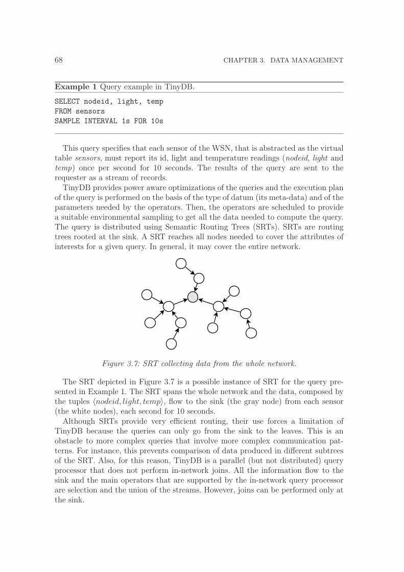
68 CHAPTER 3. DATA MANAGEMENT
Example 1 Query example in TinyDB.
SELECT nodeid, light, temp
FROM sensors
SAMPLE INTERVAL 1s FOR 10s
This query specifies that each sensor of the WSN, that is abstracted as the virtualtable sensors, must report its id, light and temperature readings (nodeid, light andtemp) once per second for 10 seconds. The results of the query are sent to therequester as a stream of records.
TinyDB provides power aware optimizations of the queries and the execution planof the query is performed on the basis of the type of datum (its meta-data) and of theparameters needed by the operators. Then, the operators are scheduled to providea suitable environmental sampling to get all the data needed to compute the query.The query is distributed using Semantic Routing Trees (SRTs). SRTs are routingtrees rooted at the sink. A SRT reaches all nodes needed to cover the attributes ofinterests for a given query. In general, it may cover the entire network.
Figure 3.7: SRT collecting data from the whole network.
The SRT depicted in Figure 3.7 is a possible instance of SRT for the query pre-sented in Example 1. The SRT spans the whole network and the data, composed bythe tuples 〈nodeid, light, temp〉, flow to the sink (the gray node) from each sensor(the white nodes), each second for 10 seconds.
Although SRTs provide very efficient routing, their use forces a limitation ofTinyDB because the queries can only go from the sink to the leaves. This is anobstacle to more complex queries that involve more complex communication pat-terns. For instance, this prevents comparison of data produced in different subtreesof the SRT. Also, for this reason, TinyDB is a parallel (but not distributed) queryprocessor that does not perform in-network joins. All the information flow to thesink and the main operators that are supported by the in-network query processorare selection and the union of the streams. However, joins can be performed only atthe sink.

3.3. DATABASE MODEL 69
3.3.2 Cougar
Cougar (Bonnet et al., 2000,Bonnet et al., 2001,Yao and Gehrke, 2002) is a WSNdatabase system developed at Cornell University and exhibits many similarities withTinyDB. The query language is a SQL dialect in which the nodes of the network arerepresented by Abstract Data Types (ADTs) with interface methods (as in objectoriented programming) to retrieve data stored in sensors.
An example of Cougar query is the following one (with similar semantics of theone presented for TinyDB):
Example 2 Query example in Cougar.
SELECT R.s.getNodeID(), R.s.getLight(), R.s.getTemp()
FROM R
WHERE $every(1);
This query specifies that each sensor of the WSN must report its id, light andtemperature readings (in ADT notation) once per second ($every(1)).
In Cougar’s queries the FROM clause can refer to a WSN’s relation. The relationincludes nodes attributes and nodes ADTs. In Example 2, the FROM clause refersto all the nodes that are collected in a set of nodes called R.
The SELECT and WHERE clauses can refer to specific node’s data and can usemethods defined in the node’s ADT. For instance, in Example 2, the temperatureof a sensor s in the relation R is denoted by the method invocation R.s.getTemp().
The query optimizer is run on a workstation and generates the query executionplan that specifies communication patterns, computational activities and tree oper-ations as joins. For each method invoked on ADTs in the query, a virtual relation iscreated. A virtual relation is a tabular representation of a method that contains theinput values and the output argument of the method it is associated with. FollowingExample 2, the method getTemp is associated with all the sensors s in the set ofsensors R, it has no input and returns a value of some suitable type, for instance afloat value to represent the sampled temperature.
3.3.3 MaD-WiSe
MaD-WiSe (Amato et al., 2005a,Amato et al., 2006a) is a recent database model forWSN. Differently from TinyDB and Cougar, its query processor is fully distributed,so that any query can be completely processed inside the network. MaD-WiSe definesan SQL-like query language, a query algebra, and a data model based on streams.
An example of MaD-WiSe query is the following:
70 CHAPTER 3. DATA MANAGEMENT
Example 3 Query example in Mad-WiSe.
SELECT roomB.Temperature
FROM roomA, roomB
WHERE roomA.Temperature > roomB.Temperature and
roomA.Temperature > 50
EVERY 10 seconds
The query specifies that the temperature of the sensors placed in two locations,called roomA and roomB, must be compared and only when the condition in theWHERE clause is true, it outputs the Temperature in roomB. The sampling of thetemperatures is performed every 10 seconds.
MaD-WiSe defines heuristics for query optimization which take into account thetransducer sampling costs, predicate selectivity and transmission costs. In the opti-mized query plan, each sensor involved in the query is assigned with a subset of theoperators. For this reason, the communication pattern between sensors involved ina query can be arbitrary, and it requires general routing strategies.
The MaD-WiSe architecture comprises a user-side module and a network-sidemodule. The user-side module implements the query parser, the query optimizer, andthe tools to inject queries and collect results. The network-side module implementsa layered architecture with a network layer, a stream system layer and a queryprocessor layer.
The network layer implements both connection oriented and connectionless ser-vices as well as a general point-to-point routing. It also embeds an energy efficiencymodule which governs the duty cycle of the sensors.
The stream system layer (Amato et al., 2006b) provides a stream abstraction to thequery processor. The streams abstract the transducers, the remote communicationsbetween nodes and the local data exchange between operators allocated on thesame node, providing a unifying view of all these sources for the underlying queryprocessor that can use them in the same way.
The query processor layer implements all the operators of the algebra, whichinclude selections, projections, spatial and temporal aggregates as well as unionsand joins. Note that the ability to perform joins within the network is unique toMaD-WiSe and allows comparison of data from different source nodes in the networkitself without the need of collecting all the data on the sink before the processing.
3.4 Data Centric Storage model
Storage systems can be used either with simple data acquisition mechanisms, or incombination with more sophisticate models such as databases. DCSs provide support

3.4. DATA CENTRIC STORAGE MODEL 71
for efficient storage of sensed/processed data and for data retrieval, and they exploitdata redundancy to ensure data reliability.
DCS addresses all the problems concerning the topology changes due to nodefailures, energy efficiency and fair load distribution using Geographic Hash Tables(GHT) (Ratnasamy et al., 2003), which are based on physical coordinates of thesensors. Other approaches to DCS, such as Graph EMbedding (GEM) (Newsomeand Song, 2003), use virtual coordinates instead of real ones. Cell Hash Routing(CHR) (Araujo et al., 2005), is another DCS system based on hash tables. CHRclusters nodes in cells of predefined and globally known shape using a distributedprotocol (e.g. dividing the sensor field in a mesh of squares) and stores each data ina cell. Moreover, K-D tree based Data-Centric Storage (KDDCS) (Aly et al., 2006)is an in-network data storage that addresses the problem of load distribution usinga distributed K-D tree (Bentley, 1975).
3.4.1 Geographic Hash Tables
A Geographic Hash Table (GHT) (Ratnasamy et al., 2003) provides a 〈key, value〉associative memory abstraction of the sensor network. Data are represented by〈key, value〉 pairs and GHT offers two operations: put and get. put(k,v) storesthe value v according to a geographic position (x, y) that is computed using the keyk. get(k) retrieves the value v that was stored using the the key k looking in theposition (x, y) computed using k.
The central part of GHT is a deterministic and uniform hash function that enablesboth put and get to find the same geographical location starting from the same keyk. The hash of the key k (h(k)) is a point (x, y) of the WSN deployment area: a〈key, value〉 pair is stored on the nodes that are closer to the point (x, y). To thispurpose GHT exploits GPSR (Karp and Kung, 2000) to route a pair 〈key, value〉towards the point (x, y) = h(key).
Home node
(x,y)
Figure 3.8: The point (x, y) (the star), the home node (the circle in black) and thehome perimeter (the circles in gray).

72 CHAPTER 3. DATA MANAGEMENT
In general, (x, y) is a generic coordinate in the deployment area and, with highprobability, does not match with any real node, as for the case depicted in Fig-ure 3.8, where the nodes of the network are the circular points and the point (x, y)is represented by a star. To deal with this problem, GHT uses the concept of homenode. The home node of (x, y) is defined as the node that is closest to the point(x, y), and it is the rendez-vous point for both put and get operations. In Figure 3.8the home node is represented by the black colored node, which is the closest one tothe point (x, y).
GHT finds the home node of (x, y) using the perimeter mode of the GPSR pro-tocol. Once a packet arrives in the proximity of the point (x, y), it is routed aroundthat point. At the end of the perimeter mode the packet returns at the starting nodeof the perimeter mode because there is no other way to reach point (x, y). This eventtriggers the home perimeter building procedure that replicates the pair 〈key, value〉on all the nodes that surround the point (x, y). The sensor that is closest to (x, y)becomes the home node. In Figure 3.8, the nodes that belong to the perimeter andthat store the datum, as well as the home node, are the gray colored nodes.
GHT provides a DCS system that is scalable and robust because in a WSN, whichnature is unreliable, these two characteristics are fundamental. GHT features datapersistence, data consistency, load distribution, database increase and topologicalgenerality. Data persistence means that a pair 〈key, value〉 that is stored in thesystem is available to queries, despite of sensors failures. Data consistency meansthat a query for a key k, is correctly routed to a node that hosts the right pair〈key, value〉. Load distribution means that the pairs 〈key, value〉 are stored in fairway such that data is not concentrated in any particular node. Database increasemeans that when new nodes are added to the system data is spread also on thenew nodes. Topological generality means that the system does not need a particulartopology to work properly.
To the purpose of data persistence and data consistency all the nodes in the homeperimeter store the pair 〈key, value〉. However, when one or more topology changesof the network occur, a home node can disappear or home perimeters can be broken.In this case, data consistency can fail because a request for a datum can be taken tothe new closest node to the point (x, y), that is neither the home node nor part of thehome perimeter. For this reason, GHT implements the Perimeter Refresh Protocol(PRP). PRP periodically generates refresh packets. Each t seconds, the home nodeperforms a put operation to the (x, y) point. The packet enters in perimeter modeand refreshes the data on the home perimeter. If the perimeter is broken, due tosome node failure, a new perimeter is built. In the same way, if new nodes aredeployed in the network, the PRP is able to compute a new home node and a newhome perimeter using both the new and the old nodes.
Each time that a node receives a refresh packet it stores the data again and setsa timer, to be notified after t seconds. This operation is necessary because, if norefresh messages arrive after t seconds, the node itself starts the refresh procedure.This ensures that a home node failure is recovered as soon as t seconds expire.

3.4. DATA CENTRIC STORAGE MODEL 73
Figure 3.9: Structured Replication (SR). The black node is the original hashed coor-dinate, the grey nodes are the level one copies and the white nodes are the level twocopies.
In GHT, if a pair 〈key, value〉 is very popular the nodes that store that value, andthe routes to them are heavily stressed. To resolve this scaling problem, GHT usesthe structured replication (SR) strategy (Figure 3.9). SR uses space decomposition.The plane is divided into a square grid and groups of contiguous areas are groupedin larger squares in a hierarchical fashion. The hierarchy is represented as a tree.The root of this tree is the whole area and the leaves are the smaller squares. Forinstance, the hierarchical decomposition depicted in Figure 3.9 shows a sensing areadivided in 16 squares. The squares are aggregated in 4 macro-squares (solid lines).With SR a pair 〈key, value〉 is still stored only in one position, this position is not(x, y) = h(key), but can be one of the in the 4d − 1 mirror points of the location(x, y). The point (x, y) is located in a squared sub-area of the grid and occupies arelative position in it, let us call it (x′, y′). A mirror point is a point, belonging to adifferent sub-area, that has the same relative coordinate (x′, y′) of the point (x, y).In Figure 3.9 the black node represents the hashed position, the gray nodes are themirrors of the second level and the white nodes are the mirrors of the third level. Anode that performs a put operation thus stores the data on a mirror node, and themirror, informs all the ancestor mirrors about the actual position of the data. Theget operation starts querying the root mirror, which propagates to its child mirrorsthe request, until the request reaches the mirror actually storing the data, that isthan returned to the querying node.
The SR does not replicates the actual datum. SR replicates the pointers to theactual position of the datum in a hierarchical way.
3.4.2 Cell Hash Routing
The Cell Hash Routing (CHR) (Araujo et al., 2005) is an evolution of GHT. CHRdivides the space in cells of equal size. Cells are squared and divide the space in

74 CHAPTER 3. DATA MANAGEMENT
a grid. Each cell defines a cluster of sensor nodes. The choice of the size of thecells is based on the communication range of the nodes. Each node in a cell mustbe able to receive messages from all the nodes in its cell and from the nodes in allthe adjacent cells. With this restriction CHR guarantees that, if the initial networkwas connected, the graph interconnecting the cells is connected too. Let r be thecommunication range of a node of the network. To enable the node to communicatewith all the nodes in its cell and with the eight adjacent cells, CHR requires that theside of a cell is at most r/
√8. CHR uses cells to solve the problem of node mobility,
that was not addressed by GHT. A cell is considered a super-node that stores somedata. If a node moves into a cell, the other nodes inside the cell replicate the datain the newcomer’s memory.
(a) Greedy routing on cells (b) Cells home-perimeter
Figure 3.10: CHR cell division of the sensors space. (a) depicts the greedy routingon the cell structure: the message is forwarded from one cell to another and when itarrives to the destination cell it is copied on all the nodes belonging to the cluster.(b) depict the case in which home cell is empty (the dark gray cell) and the datamust be stored on the home perimeter of the home cell (the light gray cells).
CHR uses a modified version of the GPSR routing protocol to route messagesfrom one node to another. The modified version of GPSR works on cells and noton single nodes. As depicted in Figure 3.10.a, to route a message from one cell toanother one, the modified GPSR routing protocol forwards the message from onecell to the following one using a single node per cell and, when the destination cellreceives the message, the receiver node copies the message in all the nodes belongingto the cell.
The choice of CHR, to use of small cells, guarantees that a node in a cell commu-nicates with all the nodes inside its cell and in the surrounding cells. The routingprotocol takes advantage of this because (i) the routing protocol is able to know ifthe cells around the actual node are empty and if it is no more possible to forwardthe message in a wanted direction and (ii) the next node, during routing from a cellto the following one, is found using a simple randomization scheme between all thenodes in the next cell.

3.4. DATA CENTRIC STORAGE MODEL 75
The cell structure itself provides two major benefits to geographic routing (in amore general fashion) because the geographic routing performs better in low densitynetworks: each hop covers a larger space and the clustered network is a less denseversion of the underlying network because each cell may contain more nodes.
Moreover, geographic routing performs better in networks which have a smallernumber of edges and enables a simpler planarization during perimeter mode. Alsoin this case the clustered network is a good choice because each cell is connectedwith all the neighbor cells.
CHR manages data storing it in a whole cluster, that is all the nodes belongingto a cell. To find out the cell that will store a datum (that is called the home cell),CHR uses a hash function to return the position where the datum must be stored to(or retrieved from). The hash function used by CHR, differently from the GHT hashfunction, does not return a point (x, y) inside the space defined by the network. TheCHR hash function returns a cell index, that refers to one of the cells in which CHRdivided the space.
In the case in which the hashed cell index points to an empty cell, as for the casedepicted in Figure 3.10.b, in which the home cell is the one in darker gray, using theGPSR perimeter mode, the messages are routed to the home cell. At this point, themessages are routed around the perimeter of the empty cell and data are stored in allthe cells that belong to the home perimeter (the cells in light gray in Figure 3.10.b).
3.4.3 Graph EMbedding
Graph EMbedding (GEM) (Newsome and Song, 2003) is an infrastructure for datacentric storage that does not need to use of geographical coordinates. GEM is basedon VPCS and the routing protocol used on this coordinate system is the VPCR.
In GEM, all the nodes have a label that enables them (i) to route the messagesfrom one node the other and (ii) to map data names to the existing labels. Thenodes are labeled using the VPCS algorithm, presented in Section 3.2.2.
In GEM, data centric storage is enabled using a hash function that maps thepair 〈key, value〉 to the embedded graph’s labels. The system uses a function h(key)to achieve this result. The function h(key) depends only on the parameter passedenabling a consistent output for all the possible senders.
The node-to-node communication is enabled using a lookup mechanism based ondata centric storage itself. If a node x wants to communicate with a node y, itneeds to know the label of y. Let us call such label L(y). At network setup, a node ycomputes both L(y) and h(y). Then it routes the message 〈y, L(y)〉 to the node withlabel h(y). When node x wants to communicate with y it sends a message to thenode h(y) to query the value L(y). After this step the node x can send the messageto y routing it to L(y).
With GEM, the user can easily add new nodes and the network is able to recon-figure to use the newcomers. When a new node enters in the network, GEM uses

76 CHAPTER 3. DATA MANAGEMENT
VPCS to assign the new node a level and an angle. In particular, a new node selectsa parent node in its neighborhood and the assigned level is the level of the parentplus one. At this point, the parent removes part of the angle range from one of itschildren and assigns it to the new node. This change affects all the child of the nodewhose range was decreased to keep the whole tree consistent.
GEM enables the user to add nodes when the network operates. Adding nodesto the network can be used to substitute broken nodes inside the network. Whena new node is added to the system, the new node chooses a parent from its setof neighbors. The parent assigns the new node a level (the parent’s level plus one)and an angle range taken away from one of the children nodes. The new node canbecome the new parent of previously disconnected nodes. In this case, the previouslydisconnected nodes start again the procedure to acquire a level and an angle fromthe new parent.
3.4.4 K-D tree based Data-Centric Storage
The K-D tree based Data-Centric Storage (KDDCS) (Aly et al., 2006) is an in-network data storage that addresses the problem of load distribution. The authorsclaim that non-uniform sensor readings, due to the presence of information hotspots inside the network (such as nodes more frequently queries than others), canbring to states of unfair load distribution in both storage and queries executionfeatures. The general idea of KDDCS is that data are stored using a distributedK-D tree (Bentley, 1975). A K-D tree is a data structure which allows logarithmicstorage and retrieval of data that are identified by geographical coordinates. TheK-D tree uses the coordinates to build a balanced tree and to guarantee poly-logaccess. In KDDCS, the K-D tree is used to provide virtual coordinates to the nodes.A virtual coordinate is a bit string of the form 11001 in which each one of the bitsrepresents the branch of the K-D tree in which the nodes is located.
KDDCS builds the K-D tree in a distributed fashion. In particular, it builds thelevels of the tree using partition lines which are constructed by a weighted split me-dian algorithm. This algorithm divides the area in regions that contain the samenumber of sensors. The weighted split median algorithm is built on top of a dis-tributed Breadth First Search (BFS) algorithm (Cormen et al., 1990). A node isfirst elected root of the BFS algorithm in a distributed way.
The election is done independently by each sensor using a probability to be theroot of the BFS. If more than one node becomes a root node, each node starts tobuild its own tree. To overcome the problem of having multiple trees, at the endonly the tree built from the root with higher id is kept.
Once the tree is built, the root proceeds in the retrieval of the coordinates of thenodes in the network, computes the median value, and communicates it to the othersensors.

3.4. DATA CENTRIC STORAGE MODEL 77
Node 0 (00)
Node 1 (01)
Node 2 (10)
Node 3 (11)
X
Y’
Y"
Figure 3.11: K-D tree built on top of a four nodes network. In the first step, the areais first divided in two using line X, in the second step each resulting sub-area of thefirst division is divided using the lines Y ′ and Y ′′. (The last step is performed inparallel on each sub-area)
The algorithm partitions recursively the network, dividing the sensor set in twobalanced parts using alternatively the x and the y values. A result of such partition-ing is depicted in Figure 3.11.
The algorithm starts partitioning the whole area horizontally. Once the medianvalue is computed and spread on the network, the sensors with y coordinate lesserthan the median value assign to themselves the coordinate 0, and the sensors withy coordinate larger than the median value assign to themselves the coordinate 1.At the second step the weighted split median algorithm is applied locally in eachsub-region. The sensors with x coordinate lesser than the median value left-shift totheir coordinate the value 0, the sensors with x coordinate greater than the medianvalue left-shift to their coordinate the value 1. The algorithm continues to divide,alternatively on the x and the y values, until each node has an unique id.
The tree that is built using this procedure is balanced because at each step thesensors set is split in two sub-sets having half of the nodes each.
Following the previous algorithm, Figure 3.11 shows an example of network thatis divided in a K-D tree structure: the first step of the algorithm divides the planein two halves following line X, thus both Node 0 and Node 1 have the first bit oftheir address set to 0 and both Node 2 and Node 3 have the first bit of their addressset to 1. The second step divides each one of the previous halves in two, followingline Y ′ and Y ′′ respectively. This last step sets the second bit of the address.
The logical coordinates built using the K-D tree are used to balance the load of

78 CHAPTER 3. DATA MANAGEMENT
the network. To provide fair load distribution the system uses a mapping betweenthe events that must be notified and this coordinate system. The mapping requiresthe events’ probability distribution. This distribution is computed during the net-work lifetime and the tree is adjusted to keep the load balanced and to pace with thecurrent distribution. At the beginning the network assumes that the events’ gener-ation probability is uniform. The mapping assigns the coordinates to specific eventranges. Consider, for instance, a network that must control temperature. KDCCSinitially guesses a possible range of values for the temperature and this range ismapped on the the virtual coordinates: when the situation evolves, and the actualrange is discovered and the mapping is corrected to balance the load again.
t
s
t’
t"L
L’
Figure 3.12: LSR routing from node s to node t using points t′ and t′′ belonging toL and L′ respectively.
KDDCS uses a routing protocol, defined into the paper itself, called Logical State-less Routing (LSR) to route the messages on the network. LSR uses the tree structureof the network to perform GPSR routing in multiple rounds. LSR uses log n roundsto route a message from one sensor to another. A sensor s that wants to send amessage to a node t must identify the least common ancestor (LCA) of both itselfand the receiver. Let R be the region that contains the LCA and let L be the linethat splits R in the two sub-regions containing s and t. s knows the position (onlyone component) of the line L because part of its address belong to this line. Themessage is routed from s to the point t′ of line L that is perpendicular to that lineusing GPSR. Once arrived at the node closer to the point t′, the procedure is re-peated, and the message is forwarded to a point t′′ belonging to L′ that is the LCAof t′ and t. Figure 3.12 shows an example of routing performed by LSR. To send apacket to node t, node s, must follow the tree structure and must use the points t′
and t′′ to route the message. Both t′ and t′′ are points belonging to the division lines
3.5. SUMMARY 79
that where used to divide the network.
3.5 Summary
In this chapter, we have presented a review of the principal topics and results indata management for WSNs.
Early WSNs were able only to perform data acquisition and to send raw datastreams, without processing, to a special node (the sink) which task was to collectthese streams and provide them to the user. More recent data management strategiesuse the network itself to provide data computation. In this way, the user is ableto program the network as a database. The network organizes itself to managesensor-to-sensor communications to compute more complex functions and to enablein-network data storage.
At the beginning of this chapter, we provided a brief introduction to the modelsof data management systems in WSNs. We actually identified four models: externalstorage, directed diffusion, data centric storage, and database models.
Then, we moved into the description of the building blocks that are essential inthe construction of an effective and efficient data management system. First of all,we described the localization systems (Savvides et al., 2001,Nasipuri and Li, 2002,Niculescu and Nath, 2003b,Niculescu and Nath, 2003a,Bulusu et al., 2000,Nagpalet al., 2003,Niculescu and Nath, 2003b,Shang and Ruml, 2004,Ji and Zha, 2004,Raoet al., 2003,Caruso et al., 2005,Cao and Abdelzaher, 2004,Newsome and Song, 2003)that are in use to provide a coordinate system to the whole network and to thesensed data. Then, we described the routing systems (Karp and Kung, 2000,Boseet al., 2001,Newsome and Song, 2003) that are essential for the reliable and efficienttransport of messages to both communicate data and to organize the infrastructureof data management. Finally, we described the redundancy mechanisms (Ratnasamyet al., 2003,Albano et al., 2007) to guarantee a more reliable storage.
After that, we described the database model (Madden et al., 2003,Madden et al.,2002a,Bonnet et al., 2000,Bonnet et al., 2001,Yao and Gehrke, 2002,Amato et al.,2005a,Amato et al., 2006a) for data management into WSNs. The database modelenables the user of the network to abstract a WSN as a database. Using this ab-straction, the user can perform queries that program the sensors to retrieve andrefine data. Then, we pointed out the two faces of the database model. The first faceshows that the database model is easy to use i.e., the ability to change the networkbehavior via queries redefinition without the need of (re)programming the network.The second face shows the limited efficiency of the system itself i.e., the cost of theflexibility must be paid in terms of complex operations executed by the network.Some database systems try to limit the inefficiency (e.g., disabling the in-networkcapability to perform join operations in a distributed fashion) at the cost of loweringof the flexibility of the systems themselves.

80 CHAPTER 3. DATA MANAGEMENT
Finally, at the end of this chapter, we focused on the data centric storage whichenables the network to work as a data storage for the data that are collected bythe sensors. This use of the network is suitable for applications in which the sinknode can be unavailable for long periods of time and between such accesses thenetwork must store the data in a reliable way. We presented different protocolsthat implement such a model, namely Geographic Hash Tables (Ratnasamy et al.,2003), Cell Hash Routing (Araujo et al., 2005), Graph EMbedding (Newsome andSong, 2003), and K-D tree based Data-Centric Storage (Aly et al., 2006). All thesesystems are based on the capability to associate a datum to a specific location insidethe network. The value used to locate a datum inside the network is given by itsassociated meta-datum.
Still focusing on the DCS, all the systems that we have seen until now do not con-sider the problem of the non-uniformity in WSNs. The only solution that mentionsnon-uniformity is KDDCS, in which the non-uniformity is seen as the presence ofhot spots inside the network.
In the next chapter, we will focus on the problem of DCS in non-uniform WSNs.Our approach to the design of a DCS system that can deal with non-uniformity canbe summarized as follows: we want to provide a system starting from the assumptionthat the network is non-uniform. Such system must work also in uniform network,without any modification and the cost of dealing with non-uniformity must be assmall as possible.
To define our non-uniformity resistant system, we start from GHT (that, as we willsee, is able to work properly only in uniform networks): we analyze GHT finding thenon-uniformity weaknesses and than we rethink it from scratch focusing on dealingwith non-uniformity. This process will bring us to a system (Q-NiGHT) that hastwo major features: (i) it is able to deal with non-uniformity and (ii) it is able toprovide a high level of fault-tolerance, using QoS associated to the data.
Apart from providing a non-uniformity proof solution to the DCS problem, weintend to use Q-NiGHT as a Trojan-horse to breakthrough into the structure ofthe non-uniformity in WSNs. To provide a solution that is able to deal with non-uniformity, we need to know how non-uniformity can influence the behavior of aWSN and we must provide countermeasures to block such influence without loosingefficiency.
From this point of view, the design of a non-uniformity proof system is similar toa chess game between the designer and the non-uniformity: a player need to preventthe winning moves of the other player without loosing the opportunity to make thegood move to win. The designer need to prevent the influence of the non-uniformitywithout loosing too much the opportunity to provide an efficient protocol.
Chapter 4
Q-NiGHT: Non-uniformity AwareData Management
Resistance does not start with big wordsBut with small deeds [...]
Asking yourself a questionAnd then asking that question to others
That is how resistance starts.- Remco Campert
Abstract
The data management in WSNs, as presented in the last chapter, is a widetopic and it is made up of different approaches and techniques. In this thesis,we choose focus on the data-centric storage model. Our main contribution inthis area is Q-NiGHT. Q-NiGHT originated by the analysis of the experi-mental results that we performed on GHT in non-uniform sensor networks.These results pointed out the inability of GHT to provide good results innon-uniformly distributed WSNs. In this chapter, we revise Q-NiGHT usingthe following approach. We start with the analysis of GHT in both uniformlyand non-uniformly distributed networks. Our aim is to point out that GHT isunable to provide good load balance in uniform networks and things get worsein non-uniform environments. GHT’s problems are due to the poor control ofthe perimeters where the data is stored on and the lack of flexibility of thehash function used to provide the coordinates of the point used to store data.Then, we move into the the study of our improvements of GHT to provide abetter load distribution. This task is achieved using two different techniques.The first one dismisses the use of perimeters to store data and the second oneuses a new, adaptive, hash function to deal with non-uniformity.
82 CHAPTER 4. Q-NIGHT: NON-UNIFORMITY AWARE DATA MANAGEMENT
In this chapter, we present Q-NiGHT∗, our approach to non-uniformity aware data-management in WSNs.
In the first part of this chapter, we analyze the characteristics of the GHT systemdescribed in Chapter 3.4.1, simulating its behavior with uniform, Gaussian and Hilldistributions of sensors.
Results show the pathological problems of GHT in non-uniform networks i.e., thelack of fair load distribution in non-uniform networks due to the religious use ofan uniform hash functions for the data distribution and the lack of control on faulttolerance issues due to the uncontrolled replication of data used by GHT.
Then we describe Q-NiGHT. We present our solution to the problem of the lackof fair load distribution with the introduction of a new class of hash functions. Thenwe present our solution to the problem of the lack of control of perimeter lengthwith the introduction of a better strategy to distribute data.
In this chapter, we do not cover the problem of how the network distribution isfound out by Q-NiGHT. We leave the description of this problem to Chapter 5,in which, we present a suite of protocols to find out networks distribution in aefficient way. These protocols are independent from Q-NiGHT and can be used inany distribution-aware sensor system.
This chapter notation. In this chapter we use a recurrent notation to identifythe actors of our research (i.e., sensors, their number, communication range and soon). Theses symbols are used across all the chapter with the meaning defined inTable 4.1. In the text sometimes we redefine some of these symbols and/or use themwith a slightly different meaning. In all these cases, we make the reader aware ofsuch changes.
s si sj generic sensorsn number of sensors in the networkr communication range of a sensorA deployment area in which sensors are locatedf geographical distribution of sensors in Ah hash function used to locate dataD datum to be stored/retrieved, in the systemM name (meta-data) for D
Table 4.1: Recurrent symbols
∗ The name Q-NiGHT stands for “Quality of service in Non-uniform Geographic Hash Tables”and it is pronounced as “knight”.

4.1. WHY DO WE NEED Q-NIGHT? 83
A note about simulations. In this chapter, we make a large use of simulations to(i) study the influence of non-uniformity on GHT and (ii) study the performanceand effectiveness of Q-NiGHT. Our simulation environment is a self-made simulatorthat is able to deal with large quantity of nodes. All the experiments are repeateduntil we achieve a statistical confidence of 95%, with a precision within 5%.
Chapter organization. This chapter is organized as follows. Section 4.1 presentsthe weaknesses of GHT, that motivate our work. Section 4.2 describes our maincontribution to data management in non-uniform networks: Q-NiGHT (publishedin (Albano et al., 2006a, Albano et al., 2006b, Albano et al., 2007)). Section 4.3describes an application of Q-NiGHT in the field of resource localization inside anheterogeneous WSN (published in (Nidito et al., 2007)). Finally, Section 4.4 drawsthe conclusions of the research work described in this chapter.
4.1 Why do we need Q-NiGHT?
GHT (Ratnasamy et al., 2003) implements Data Centric Storage using GeographicHash Tables and the GPSR protocol. We have already discussed how the protocolworks in Chapter 3.4.1. Here, we discuss the behavior of GHT, with respect to loaddistribution. In particular, we describe a simulation experiment that gives betterinsights on the protocol behavior and settles some motivations for Q-NiGHT.
The first thing that we want to measure is the mean and the variance of theperimeters found by GHT. As GHT stores a datum on all the perimeter surroundingthe corresponding hash coordinates, this measure gives us an idea on the number ofcopies of each datum stored by GHT.
Our experiment is organized as follows. In order to measure the degree of unbal-ance of GHT, we simulated a flat square sensing field, with a 1000m side. Each nodehas circular transmission range with 30m radius. In this area, we simulated severalWSNs ranging from 5000 to 20000 sensors. For each network size, we randomlygenerate 100 networks with uniform distribution. For each network, we computethe mean and the variance of the number of nodes found in a GPSR perimeter asfollows. For each sensor network the simulator uniformly selects 1000 points and,for each point, it computes the number of nodes in the perimeter surrounding thepoint. GPSR need to work with a planar graph in order the perimeter mode tobehave correctly, thus, in our experiments we use both GG and RNG planarization.
Figure 4.1.a and Figure 4.1.b show the mean and variance of the perimeter lengthused to store data by GHT. Figure 4.1.a shows the length of such perimeter foundout using GG planarization and Figure 4.1.b shows the length of such perimeterfound out using RNG planarization.
Both Figure 4.1.a and Figure 4.1.b show that the lenght of the perimeters ishighly variable. This is even more evident if we compare the standard deviation of
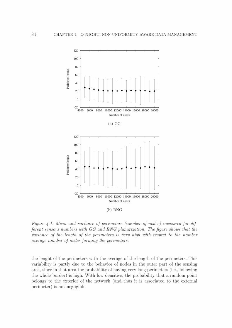
84 CHAPTER 4. Q-NIGHT: NON-UNIFORMITY AWARE DATA MANAGEMENT
-20
0
20
40
60
80
100
120
4000 6000 8000 10000 12000 14000 16000 18000 20000
Peri
met
er le
ngth
Number of nodes
(a) GG
-20
0
20
40
60
80
100
120
4000 6000 8000 10000 12000 14000 16000 18000 20000
Peri
met
er le
ngth
Number of nodes
(b) RNG
Figure 4.1: Mean and variance of perimeters (number of nodes) measured for dif-ferent sensors numbers with GG and RNG planarization. The figure shows that thevariance of the length of the perimeters is very high with respect to the numberaverage number of nodes forming the perimeters.
the lenght of the perimeters with the average of the length of the perimeters. Thisvariability is partly due to the behavior of nodes in the outer part of the sensingarea, since in that area the probability of having very long perimeters (i.e., followingthe whole border) is high. With low densities, the probability that a random pointbelongs to the exterior of the network (and thus it is associated to the externalperimeter) is not negligible.
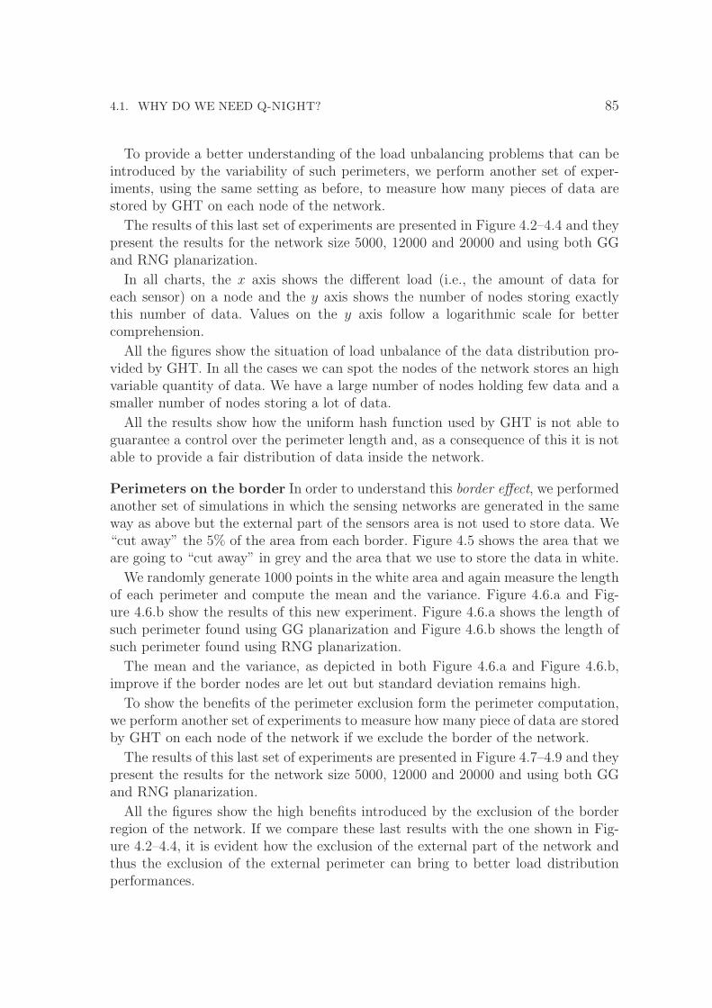
4.1. WHY DO WE NEED Q-NIGHT? 85
To provide a better understanding of the load unbalancing problems that can beintroduced by the variability of such perimeters, we perform another set of exper-iments, using the same setting as before, to measure how many pieces of data arestored by GHT on each node of the network.
The results of this last set of experiments are presented in Figure 4.2–4.4 and theypresent the results for the network size 5000, 12000 and 20000 and using both GGand RNG planarization.
In all charts, the x axis shows the different load (i.e., the amount of data foreach sensor) on a node and the y axis shows the number of nodes storing exactlythis number of data. Values on the y axis follow a logarithmic scale for bettercomprehension.
All the figures show the situation of load unbalance of the data distribution pro-vided by GHT. In all the cases we can spot the nodes of the network stores an highvariable quantity of data. We have a large number of nodes holding few data and asmaller number of nodes storing a lot of data.
All the results show how the uniform hash function used by GHT is not able toguarantee a control over the perimeter length and, as a consequence of this it is notable to provide a fair distribution of data inside the network.
Perimeters on the border In order to understand this border effect, we performedanother set of simulations in which the sensing networks are generated in the sameway as above but the external part of the sensors area is not used to store data. We“cut away” the 5% of the area from each border. Figure 4.5 shows the area that weare going to “cut away” in grey and the area that we use to store the data in white.
We randomly generate 1000 points in the white area and again measure the lengthof each perimeter and compute the mean and the variance. Figure 4.6.a and Fig-ure 4.6.b show the results of this new experiment. Figure 4.6.a shows the length ofsuch perimeter found using GG planarization and Figure 4.6.b shows the length ofsuch perimeter found using RNG planarization.
The mean and the variance, as depicted in both Figure 4.6.a and Figure 4.6.b,improve if the border nodes are let out but standard deviation remains high.
To show the benefits of the perimeter exclusion form the perimeter computation,we perform another set of experiments to measure how many piece of data are storedby GHT on each node of the network if we exclude the border of the network.
The results of this last set of experiments are presented in Figure 4.7–4.9 and theypresent the results for the network size 5000, 12000 and 20000 and using both GGand RNG planarization.
All the figures show the high benefits introduced by the exclusion of the borderregion of the network. If we compare these last results with the one shown in Fig-ure 4.2–4.4, it is evident how the exclusion of the external part of the network andthus the exclusion of the external perimeter can bring to better load distributionperformances.
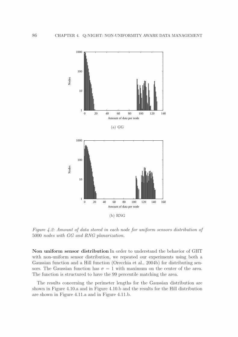
86 CHAPTER 4. Q-NIGHT: NON-UNIFORMITY AWARE DATA MANAGEMENT
1
10
100
1000
0 20 40 60 80 100 120 140
Nod
es
Amount of data per node
(a) GG
1
10
100
1000
0 20 40 60 80 100 120 140 160
Nod
es
Amount of data per node
(b) RNG
Figure 4.2: Amount of data stored in each node for uniform sensors distribution of5000 nodes with GG and RNG planarization.
Non uniform sensor distribution In order to understand the behavior of GHTwith non-uniform sensor distribution, we repeated our experiments using both aGaussian function and a Hill function (Orecchia et al., 2004b) for distributing sen-sors. The Gaussian function has σ = 1 with maximum on the center of the area.The function is structured to have the 99 percentile matching the area.
The results concerning the perimeter lengths for the Gaussian distribution areshown in Figure 4.10.a and in Figure 4.10.b and the results for the Hill distributionare shown in Figure 4.11.a and in Figure 4.11.b.
4.1. WHY DO WE NEED Q-NIGHT? 87
1
10
100
1000
10000
0 10 20 30 40 50 60 70
Nod
es
Amount of data per node
(a) GG
1
10
100
1000
10000
0 10 20 30 40 50 60 70 80 90
Nod
es
Amount of data per node
(b) RNG
Figure 4.3: Amount of data stored in each node for uniform sensors distribution of12000 nodes with GG and RNG planarization.
All the results show a behavior that is much worse than the one shown withuniform distribution because GHT uses a uniform hash function independently ofthe real distribution of the sensors.
The results concerning the load distribution are presented in Figures 4.12–4.14and they present the results for Gaussian and Hill distributed networks of size 5000,12000 and 20000.
All the figures show how the use of the uniform hashing function bring to a stateof high unbalance in load distribution, much times worse than the one presented in

88 CHAPTER 4. Q-NIGHT: NON-UNIFORMITY AWARE DATA MANAGEMENT
1
10
100
1000
10000
100000
0 10 20 30 40 50 60
Nod
es
Amount of data per node
(a) GG
1
10
100
1000
10000
0 10 20 30 40 50 60 70 80
Nod
es
Amount of data per node
(b) RNG
Figure 4.4: Amount of data stored in each node for uniform sensors distribution of20000 nodes with GG and RNG planarization.
Figures 4.2–4.4.
This brings to a pathological state of load unbalance that is due to the differentamount of data that must be managed by an equal number of sensors: a sensorbelonging to a sparser region the deployment area must manage a quantity of datathat is larger than the quantity managed by a sensor inside a denser part of thenetwork.
Load unbalance and QoS. Another issue with GHT is that there is no way tocontrol the QoS provided for each datum. Since the point (x, y) on which a datum

4.2. Q-NIGHT 89
Figure 4.5: The border area (grey) and the storing area (white).
should be stored is obtained computing a hash function h on its associated meta-data M , the selection of the sensors candidate for storage is in practice independentfrom the importance of the datum.
In principle, this ensures the same treatment for each stored datum. However,if the meta-datum M is particularly popular and many sensors generate the datadescribed by M , the sensors located in the perimeter around (x, y) = h(M) wouldbe burdened with a high storage and communication load.
For this reason, the authors of GHT introduce the technique of structured replica-tion (Ratnasamy et al., 2003), that replicates the same datum in different sub-areasof the sensing field. However neither GHT nor structured replication ensure that thelevel of redundancy associated to a datum is related to the importance of the datumitself: GHT assures only the same average treatment of each stored datum.
Another aspect is that, although the average level of redundancy of the meta-datum is constant, in practice it can vary significantly (due to the fact that eachgeographic point is surrounded by a different perimeter), even in case of uniformdistribution of the sensors.
4.2 Q-NiGHT
In this section we present Q-NiGHT, a novel DCS protocol which moves fromGHT incorporating QoS control and featuring good load balance among sensorsdistributed in a non-uniform way.
Q-NiGHT uses a strategy similar to the rejection method (Neumann, 1951) tobuild a hash function biased with sensor distribution. This spreads data more evenlyamong nodes. In addition, Q-NiGHT can provide QoS with different redundancytechniques. We first detail the protocol using pure replication, allowing the user to

90 CHAPTER 4. Q-NIGHT: NON-UNIFORMITY AWARE DATA MANAGEMENT
4
6
8
10
12
14
16
4000 6000 8000 10000 12000 14000 16000 18000 20000
Peri
met
er le
ngth
Number of nodes
(a) GG
4
6
8
10
12
14
16
4000 6000 8000 10000 12000 14000 16000 18000 20000
Peri
met
er le
ngth
Number of nodes
(b) RNG
Figure 4.6: Mean and variance of perimeters (number of nodes) measured for dif-ferent sensors numbers with GG and RNG planarization without considering theborders of the network. The figure shows a lower length of the perimeters with re-spect to the results presented in Figure 4.1.
choose the number of replicas required for a given datum. however all replicationmethods discussed in Chapter 3 can be used.
Then, we conduct detailed simulations of Q-NiGHT and analyze the resultsobtained with respect to the load of each sensor (i.e., the number of data storedin each node) and the number of messages needed for data storage and retrieval.Results show a good performance of Q-NiGHT on different sensors distributions

4.2. Q-NIGHT 91
1
10
100
1000
10000
0 5 10 15 20
Nod
es
Amount of data per node
(a) GG
1
10
100
1000
0 5 10 15 20 25 30 35 40
Nod
es
Amount of data per node
(b) RNG
Figure 4.7: Amount of data stored in each node for uniform sensors distribution of5000 nodes with GG and RNG planarization without considering the borders of thenetwork.
on terms of both protocol costs and load distribution.
4.2.1 A first step: GHT with non-uniform hashing
As we have seen, a serious problem with GHT is the fact that it uses a uniform hashfunction independently of the real distribution of sensors. This leads to a poor controlon the perimeter lengths as shown in Figures 4.10–4.11 and to the pathological state

92 CHAPTER 4. Q-NIGHT: NON-UNIFORMITY AWARE DATA MANAGEMENT
1
10
100
1000
10000
0 1 2 3 4 5 6 7 8 9
Nod
es
Amount of data per node
(a) GG
1
10
100
1000
10000
0 2 4 6 8 10 12 14
Nod
es
Amount of data per node
(b) RNG
Figure 4.8: Amount of data stored in each node for uniform sensors distribution of12000 nodes with GG and RNG planarization without considering the borders of thenetwork.
of unbalancing in load distribution, as shown in Figures 4.12–4.14.
In this section, we explore what happens if we use hash functions which scatterdata approximately with the same distribution of the sensors. We can observe thata hash function h(k) is a kind of pseudo-random number generator: starting froma seed (in our case the key k) it produces an output (in our case in a value inR2) such that for near values of the key the hashed values must be distant. Withthis consideration in mind we define a new hash function, whose pseudo-code is

4.2. Q-NIGHT 93
1
10
100
1000
10000
100000
0 1 2 3 4 5 6 7
Nod
es
Amount of data per node
(a) GG
1
10
100
1000
10000
0 2 4 6 8 10
Nod
es
Amount of data per node
(b) RNG
Figure 4.9: Amount of data stored in each node for uniform sensors distribution of20000 nodes with GG and RNG planarization without considering the borders of thenetwork.
shown in Algorithm 2. This function uses a strategy similar to the one used in therejection method (Neumann, 1951), but with some differences. Rejection method is atechnique used in random number generation to produce random numbers followingany probability distribution, with limited dominion.
The basic idea is the following. Let us suppose to have a probability functionand an interval (a, b) in which we want to generate random numbers, as depicted inFigure 4.15.
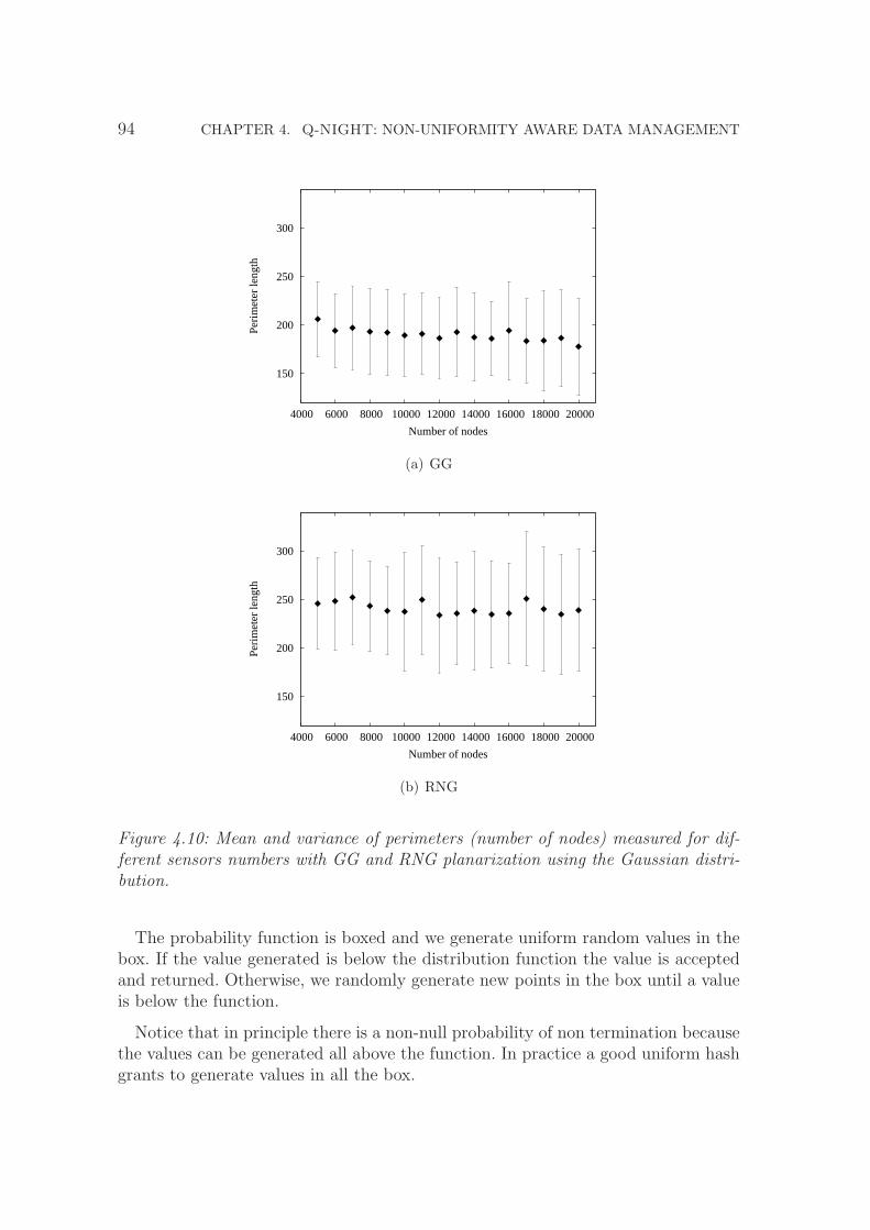
94 CHAPTER 4. Q-NIGHT: NON-UNIFORMITY AWARE DATA MANAGEMENT
150
200
250
300
4000 6000 8000 10000 12000 14000 16000 18000 20000
Peri
met
er le
ngth
Number of nodes
(a) GG
150
200
250
300
4000 6000 8000 10000 12000 14000 16000 18000 20000
Peri
met
er le
ngth
Number of nodes
(b) RNG
Figure 4.10: Mean and variance of perimeters (number of nodes) measured for dif-ferent sensors numbers with GG and RNG planarization using the Gaussian distri-bution.
The probability function is boxed and we generate uniform random values in thebox. If the value generated is below the distribution function the value is acceptedand returned. Otherwise, we randomly generate new points in the box until a valueis below the function.
Notice that in principle there is a non-null probability of non termination becausethe values can be generated all above the function. In practice a good uniform hashgrants to generate values in all the box.

4.2. Q-NIGHT 95
0
50
100
150
200
250
300
350
4000 6000 8000 10000 12000 14000 16000 18000 20000
Peri
met
er le
ngth
Number of nodes
(a) GG
0
50
100
150
200
250
300
350
4000 6000 8000 10000 12000 14000 16000 18000 20000
Peri
met
er le
ngth
Number of nodes
(b) RNG
Figure 4.11: Mean and variance of perimeters (number of nodes) measured for dif-ferent sensors numbers with GG and RNG planarization using the Hill distribution.
From its key k, the function RejectionHash returns a pair (x, y) of coordinateswhere to place data, belonging to distribution f . Instead of using uniform random-ization to provide the points inside the box, RejectionHash uses uniform hashingon the key. At each iteration, if necessary, it changes lightly the key in a determin-istic way. This operation is represented by the increment of the key k of a quantityi that is increased at each iteration. This operation is needed to guarantee that ateach iteration we provide a new, and very different, uniformly hashed vale.
In order to understand the goodness of RejectionHash function we repeated

96 CHAPTER 4. Q-NIGHT: NON-UNIFORMITY AWARE DATA MANAGEMENT
1
10
100
1000
10000
0 200 400 600 800 1000 1200 1400
Nod
es
Amount of data per node
(a) Gaussian
1
10
100
1000
10000
0 100 200 300 400 500 600 700
Nod
es
Amount of data per node
(b) Hill
Figure 4.12: Amount of data stored in each node by GHT for the Gaussian and Hillsensors distribution of 5000 nodes.
our experiments presented in Figures 4.10–4.11 and in Figures 4.12–4.14 using theRejectionHash function instead of the uniform GHT hash function.
The results showing the mean and the variance of the length of the perimetersfor the Gaussian distribution are shown in Figure 4.16 and the results for the Hilldistribution are shown in Figure 4.17.
Both Figure 4.16 and Figure 4.17 show the good behavior of the non-uniform hashfunction. RejectionHash fits well the sensors distribution in the data dissemina-tion strategy with a good global load distribution.

4.2. Q-NIGHT 97
1
10
100
1000
10000
0 200 400 600 800 1000 1200
Nod
es
Amount of data per node
(a) Gaussian
1
10
100
1000
10000
0 50 100 150 200 250 300
Nod
es
Amount of data per node
(b) Hill
Figure 4.13: Amount of data stored in each node by GHT for the Gaussian and Hillsensors distribution of 12000 nodes.
These results are even better than the results provided with uniform distributionand uniform hashing (Figure 4.1 and Figure 4.6). This is due to the nature of non-uniform distributions themselves.
A non-uniform distribution tends to have parts of the network that are moredense than others. RejectionHash function distributes more data in these region.As happened in the uniform case, the perimeters get shorter in larger, and thusdenser, networks because the nodes are closer and few nodes are needed to form aperimeter around a point.

98 CHAPTER 4. Q-NIGHT: NON-UNIFORMITY AWARE DATA MANAGEMENT
1
10
100
1000
10000
100000
0 100 200 300 400 500 600 700 800 900 1000
Nod
es
Amount of data per node
(a) Gaussian
1
10
100
1000
10000
100000
0 20 40 60 80 100 120 140 160 180
Nod
es
Amount of data per node
(b) Hill
Figure 4.14: Amount of data stored in each node by GHT for the Gaussian and Hillsensors distribution of 20000 nodes.
The evidence of these results is more clear if we look at Figures 4.18–4.20. Thislast set of experiments show the quantity of data stored in each node by GHT if ituses RejectionHash instead of the uniform hash function.
Figures 4.18–4.20 show a big improvement in the load distribution of GHT, withrespect to the results presented in Figures 4.12–4.14. Even if GHT still the perimetersto store data in the network, the use of a hash function that is able to provide thedata coordinates with a distribution biased on the network distribution shows bigimprovements.
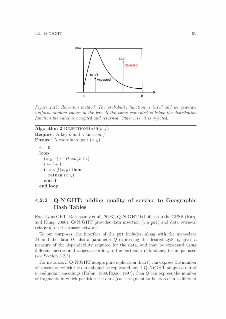
4.2. Q-NIGHT 99
a b
(x,y)
(x’,y’)
max
Rejected
Accepted
Figure 4.15: Rejection method: The probability function is boxed and we generateuniform random values in the box. If the value generated is below the distributionfunction the value is accepted and returned. Otherwise, it is rejected.
Algorithm 2 RejectionHash(k, f)
Require: A key k and a function f .Ensure: A coordinate pair (x, y).
i ← 0loop
(x, y, z) ← Hash(k + i)i ← i + 1if z < f(x, y) then
return (x, y)end if
end loop
4.2.2 Q-NiGHT: adding quality of service to GeographicHash Tables
Exactly as GHT (Ratnasamy et al., 2003), Q-NiGHT is built atop the GPSR (Karpand Kung, 2000). Q-NiGHT provides data insertion (via put) and data retrieval(via get) on the sensor network.
To our purposes, the interface of the put includes, along with the meta-dataM and the data D, also a parameter Q expressing the desired QoS. Q gives ameasure of the dependability required for the data, and may be expressed usingdifferent metrics and ranges according to the particular redundancy technique used(see Section 3.2.3).
For instance, if Q-NiGHT adopts pure replication then Q can express the numberof sensors on which the data should be replicated, or, if Q-NiGHT adopts n out ofm redundant encodings (Rabin, 1989,Rizzo, 1997), then Q can express the numberof fragments in which partition the data (each fragment to be stored in a different

100 CHAPTER 4. Q-NIGHT: NON-UNIFORMITY AWARE DATA MANAGEMENT
-10
0
10
20
30
40
50
60
70
4000 6000 8000 10000 12000 14000 16000 18000 20000
Peri
met
er le
ngth
Number of nodes
(a) GG
-10
0
10
20
30
40
50
60
70
4000 6000 8000 10000 12000 14000 16000 18000 20000
Peri
met
er le
ngth
Number of nodes
(b) RNG
Figure 4.16: Mean and variance of perimeters (number of nodes) measured for dif-ferent sensors numbers with GG and RNG planarization using the Gaussian distri-bution and the RejectionHash hashing function.
sensor) and the number of redundant fragments.
In the following, we describe Q-NiGHT assuming pure replication of the data.Data insertion is expressed with put(M,D,Q). We assume Q ranges in [1, Qmax] andgives the number of sensors on which the data should be replicated. Let s be thesource node of a put(M,D,Q) operation. s first computes h(M), where h is the Re-
jectionHash function conditioned with the sensor distribution function, f , in thesensing field, as discussed in Section 4.2.1. h(M) returns a pair of geographic coor-

4.2. Q-NIGHT 101
-20
0
20
40
60
80
100
120
140
160
4000 6000 8000 10000 12000 14000 16000 18000 20000
Peri
met
er le
ngth
Number of nodes
(a) GG
-20
0
20
40
60
80
100
120
140
160
4000 6000 8000 10000 12000 14000 16000 18000 20000
Peri
met
er le
ngth
Number of nodes
(b) RNG
Figure 4.17: Mean and variance of perimeters (number of nodes) measured for dif-ferent sensors numbers with GG and RNG planarization using the Hill distributionand the RejectionHash hashing function.
dinates (x, y) as the destination of the packet Pp=<(x,y),<M,D,Q>>. The packet inturn is sent to the destination using the GPSR protocol. As in GHT, we call homenode the sensor sd (of coordinates (x′, y′)) geographically closest to the destinationcoordinates. The home node naturally receives the packet as a consequence of ap-plying GPSR. Upon the reception of packet Pp, sensor sd begins a dispersal protocolwhich selects Q sensors to store a copy of <M,D>.
The dispersal protocol is iterative and uses the concept of ball. Given a sensor sd
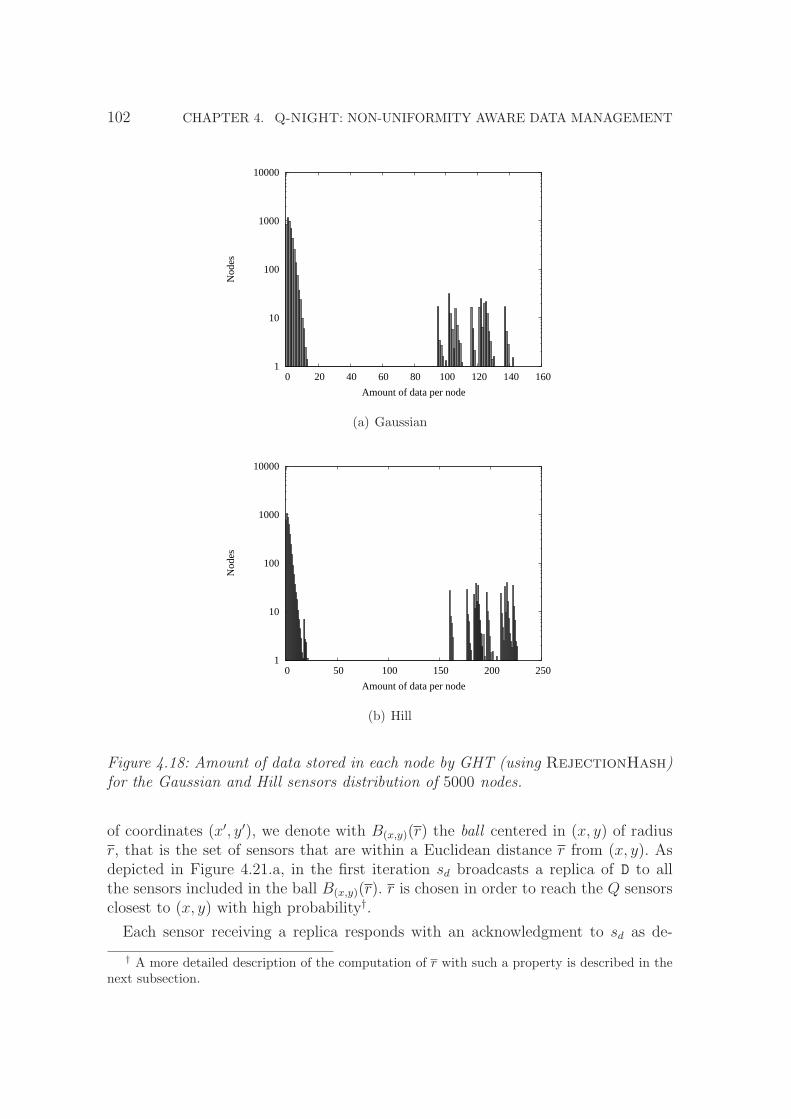
102 CHAPTER 4. Q-NIGHT: NON-UNIFORMITY AWARE DATA MANAGEMENT
1
10
100
1000
10000
0 20 40 60 80 100 120 140 160
Nod
es
Amount of data per node
(a) Gaussian
1
10
100
1000
10000
0 50 100 150 200 250
Nod
es
Amount of data per node
(b) Hill
Figure 4.18: Amount of data stored in each node by GHT (using RejectionHash)for the Gaussian and Hill sensors distribution of 5000 nodes.
of coordinates (x′, y′), we denote with B(x,y)(r) the ball centered in (x, y) of radiusr, that is the set of sensors that are within a Euclidean distance r from (x, y). Asdepicted in Figure 4.21.a, in the first iteration sd broadcasts a replica of D to allthe sensors included in the ball B(x,y)(r). r is chosen in order to reach the Q sensorsclosest to (x, y) with high probability†.
Each sensor receiving a replica responds with an acknowledgment to sd as de-
† A more detailed description of the computation of r with such a property is described in thenext subsection.

4.2. Q-NIGHT 103
1
10
100
1000
10000
0 10 20 30 40 50 60 70
Nod
es
Amount of data per node
(a) Gaussian
1
10
100
1000
10000
0 10 20 30 40 50 60 70 80 90 100
Nod
es
Amount of data per node
(b) Hill
Figure 4.19: Amount of data stored in each node by GHT (using RejectionHash)for the Gaussian and Hill sensors distribution of 12000 nodes.
picted in Figure 4.21.b. Finally, sensor sd confirms the Q − 1 acknowledgmentsreceived from the sensors geographically nearest to (x, y) and disregards the others(Figure 4.21.c). The confirmation requires an extra packet sent by sd. Sensors whichreceive the confirmation keep the datum while the others will disregard the dataafter a timeout. If sd receives Q′ < Q acknowledgments, then it executes anotheriteration of the dispersal protocol with r = 2r in which it considers only the sensorsin B(x′,y′)(2r) − B(x′,y′)(r). The dispersal protocol stops as soon as Q sensors havebeen hired or the outermost perimeter has been reached. The dispersal protocol is

104 CHAPTER 4. Q-NIGHT: NON-UNIFORMITY AWARE DATA MANAGEMENT
1
10
100
1000
10000
100000
0 2 4 6 8 10 12 14 16 18
Nod
es
Amount of data per node
(a) Gaussian
1
10
100
1000
10000
100000
0 2 4 6 8 10 12 14 16
Nod
es
Amount of data per node
(b) Hill
Figure 4.20: Amount of data stored in each node by GHT (using RejectionHash)for the Gaussian and Hill sensors distribution of 20000 nodes.
a simple implementation of a geo-casting protocol (Seada and Helmy, 2006).
When a node sg of coordinates (r, z) executes get(M), it first computes (x, y) =h(M), and then sends a query packet Pg=<(x,y),<(r,z),M>> using the GPSR pro-tocol. In turn, packet Pg will reach the perimeter surrounding (x, y) and it will startto move across the perimeter. Eventually, the packet will reach either the home nodeor another node containing a replica of the data D associated to M . This node willstop packet Pg and will send the required data back to sg.
The complexity of the put protocol clearly depends upon the choice of r as this

4.2. Q-NIGHT 105
(a) Broadcast phase (b) Replay of the nodesinside B(x,y)(r)
(c) Choice of the closestsensors
Figure 4.21: Dispersal protocol of a datum D with Q = 3 and (x, y) = h(M) (rep-resented by the star in the three pictures). (a) The home node (shaded) broadcastsD up to distance r. (b) The nodes inside the B(x,y)(r) replay to the home node. (c)The home node sends the confirmation to the Q − 1 closest nodes.
determines the number of iterations made to successfully place the Q replicas.
In order to evaluate our solution, using the ball instead of the perimeter to storedata, we perform simulations to check the quantity of data stored in each node.As before, we simulate a flat square sensing field, with a 1000m side. Each nodehas circular transmission range with 30m radius. In this area, we simulated severalWSNs made up of 5000, 12000 and 20000 sensors, using both RNG and GG toplanarize the networks during GPSR perimeter modes. For each network size, werandomly generated 100 networks with uniform, Gaussian and Hill distributions,and performed 2000 put operations with uniformly generated meta-data using bothGHT and Q-NiGHT. In these trials, Q-NiGHT uses a pure replication QoS with15 replicas for each datum.
In all charts, the x axis shows the different load (i.e., the number of pieces of datastored) on a node and the y axis shows the number of nodes storing exactly thisnumber of pieces of data. Values on the y axis follow a logarithmic scale for bettercomprehension.
Figures 4.22–4.24 show the quantity of data stored in each node for uniform,Gaussian and Hill sensors distributions of a network made up of 5000 sensors usingRejectionHash and the Q-NiGHT dispersal protocol.
If we compare Figures 4.22–4.24 with their counterparts that do not use thedispersal protocol, namely Figure 4.2, Figure 4.7, Figure 4.12 and Figure 4.18, wecan notice that Q-NiGHT reaches better load balance than GHT, even in theuniform case. In all the cases, GHT shows its unbalance problems, while Q-NiGHT
manages to balance the load. The reason of such a behavior, is that GHT storesdata on perimeters and since such perimeters are chosen arbitrarily, GHT producesvery unbalanced storages.

106 CHAPTER 4. Q-NIGHT: NON-UNIFORMITY AWARE DATA MANAGEMENT
1
10
100
1000
0 2 4 6 8 10 12 14 16 18
Nod
es
Amount of data per node
(a) GG
1
10
100
1000
0 2 4 6 8 10 12 14 16 18
Nod
es
Amount of data per node
(b) RNG
Figure 4.22: Amount of data stored in each node for uniform sensors distribution of5000 nodes using RejectionHash and the Q-NiGHT dispersal protocol.
For instance, comparing Figure 4.22 (the uniform case) with Figure 4.2, the differ-ences are very large. We can spot the following interesting situation: a large numberof nodes store few data (approximatively between 0 and 25 data for each node) andat the same time, in the same network, we have good number of nodes storing alot of data (approximatively between 100 and 150 data for each node). This storageconfiguration finds its explanation in the use of the external perimeter to store data.
On the other hand, Q-NiGHT stores almost the same number of data on eachnode (approximatively between 0 and 18 data for each node) because Q-NiGHT

4.2. Q-NIGHT 107
1
10
100
1000
0 2 4 6 8 10 12 14 16 18
Nod
es
Amount of data per node
(a) GG
1
10
100
1000
0 2 4 6 8 10 12 14 16 18 20
Nod
es
Amount of data per node
(b) RNG
Figure 4.23: Amount of data stored in each node for Gaussian sensors distributionof 5000 nodes using RejectionHash and the Q-NiGHT dispersal protocol.
looks for a fixed number Q of storage nodes for each datum and it is much moredifficult for the same node to store a large number of different data.
The difference is smaller if we compare Figure 4.22 with Figure 4.7, in this lastcase the network do not use the external perimeter to store data and thus, GHTfinds smaller perimeters, with size comparable to our Q.
The different behaviors of Q-NiGHT and GHT are more evident in non-uniformnetworks (Figures 4.23–4.24). If we compare Figures 4.23–4.24 with Figure 4.12 andFigure 4.18, we can easily see the great advantage of using both the Rejection-

108 CHAPTER 4. Q-NIGHT: NON-UNIFORMITY AWARE DATA MANAGEMENT
1
10
100
1000
0 2 4 6 8 10 12 14 16 18 20
Nod
es
Amount of data per node
(a) GG
1
10
100
1000
0 5 10 15 20 25
Nod
es
Amount of data per node
(b) RNG
Figure 4.24: Amount of data stored in each node for Hill sensors distribution of 5000nodes using RejectionHash and the Q-NiGHT dispersal protocol.
Hash, to locate data accordingly to the network distribution and thus preventingto use sparser regions of the network and the use of the dispersal protocol to spreaddata on a limited number of nodes.
Figures 4.25–4.27 show the quantity of data stored in each node for uniform,Gaussian and Hill sensors distributions of a network made up of 12000 sensors usingRejectionHash and the Q-NiGHT dispersal protocol.
Finally, Figures 4.28–4.30 show the quantity of data stored in each node for uni-form, Gaussian and Hill sensors distributions of a network made up of 20000 sensors
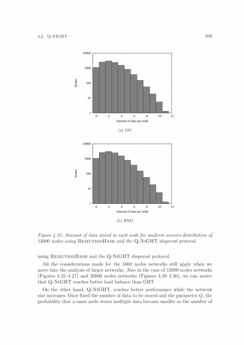
4.2. Q-NIGHT 109
1
10
100
1000
10000
0 2 4 6 8 10 12
Nod
es
Amount of data per node
(a) GG
1
10
100
1000
10000
0 2 4 6 8 10 12
Nod
es
Amount of data per node
(b) RNG
Figure 4.25: Amount of data stored in each node for uniform sensors distribution of12000 nodes using RejectionHash and the Q-NiGHT dispersal protocol.
using RejectionHash and the Q-NiGHT dispersal protocol.
All the considerations made for the 5000 nodes networks still apply when wemove into the analysis of larger networks. Also in the case of 12000 nodes networks(Figures 4.25–4.27) and 20000 nodes networks (Figures 4.28–4.30), we can noticethat Q-NiGHT reaches better load balance than GHT.
On the other hand, Q-NiGHT, reaches better performance while the networksize increases. Once fixed the number of data to be stored and the parameter Q, theprobability that a same node stores multiple data become smaller as the number of

110 CHAPTER 4. Q-NIGHT: NON-UNIFORMITY AWARE DATA MANAGEMENT
1
10
100
1000
10000
0 2 4 6 8 10 12
Nod
es
Amount of data per node
(a) GG
1
10
100
1000
10000
0 2 4 6 8 10 12
Nod
es
Amount of data per node
(b) RNG
Figure 4.26: Amount of data stored in each node for Gaussian sensors distributionof 12000 nodes using RejectionHash and the Q-NiGHT dispersal protocol.
nodes inside the network increases.
r computation. We now discuss how to compute the radius r of the ball used bythe Q-NiGHT dispersal protocol to choose the nodes to store data in.
Let f be the sensor probability distribution function, Q an integer in [1, Qmax],and (x, y) a point in R2 we want to fix r in such a way that, called SB the setof sensors laying in the space defined by the ball B(x,y)(r), |SB| ≥ Q with highprobability.

4.2. Q-NIGHT 111
1
10
100
1000
10000
0 2 4 6 8 10 12
Nod
es
Amount of data per node
(a) GG
1
10
100
1000
10000
0 2 4 6 8 10 12
Nod
es
Amount of data per node
(b) RNG
Figure 4.27: Amount of data stored in each node for Hill sensors distribution of12000 nodes using RejectionHash and the Q-NiGHT dispersal protocol.
We first discuss the intuition behind our approximation schema. Let Ar denotethe circle of radius r, we want to fix r such that
E[number of sensors ∈ Ar] = Q (4.2.1)
Equation (4.2.1) can be rewritten in terms of the probability f
n ·∫
Ar
f(x, y)dAr = Q (4.2.2)

112 CHAPTER 4. Q-NIGHT: NON-UNIFORMITY AWARE DATA MANAGEMENT
1
10
100
1000
10000
0 1 2 3 4 5 6 7 8 9
Nod
es
Amount of data per node
(a) GG
1
10
100
1000
10000
0 1 2 3 4 5 6 7 8
Nod
es
Amount of data per node
(b) RNG
Figure 4.28: Amount of data stored in each node for uniform sensors distribution of20000 nodes using RejectionHash and the Q-NiGHT dispersal protocol.
where n is the total number of sensors in the network and the integral representsthe probability to have a sensor in Ar. Direct computation of the integral above islikely to need a large number of floating point operations in practical distributions.
To simplify the computation of r, we use the following strategy. Instead of usingAr ,we use the square inscribed in the circle of radius r. This square has edge r
√2
and area A′r = 2r2. If we impose to have Q nodes in A′
r, we grant at least Q nodes
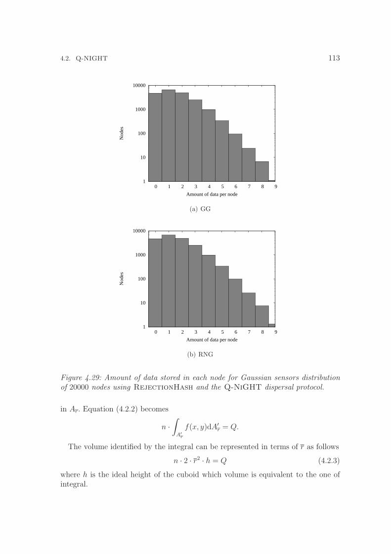
4.2. Q-NIGHT 113
1
10
100
1000
10000
0 1 2 3 4 5 6 7 8 9
Nod
es
Amount of data per node
(a) GG
1
10
100
1000
10000
0 1 2 3 4 5 6 7 8 9
Nod
es
Amount of data per node
(b) RNG
Figure 4.29: Amount of data stored in each node for Gaussian sensors distributionof 20000 nodes using RejectionHash and the Q-NiGHT dispersal protocol.
in Ar. Equation (4.2.2) becomes
n ·∫
A′
r
f(x, y)dA′r = Q.
The volume identified by the integral can be represented in terms of r as follows
n · 2 · r2 · h = Q (4.2.3)
where h is the ideal height of the cuboid which volume is equivalent to the one ofintegral.

114 CHAPTER 4. Q-NIGHT: NON-UNIFORMITY AWARE DATA MANAGEMENT
1
10
100
1000
10000
0 2 4 6 8 10 12
Nod
es
Amount of data per node
(a) GG
1
10
100
1000
10000
0 2 4 6 8 10 12
Nod
es
Amount of data per node
(b) RNG
Figure 4.30: Amount of data stored in each node for Hill sensors distribution of20000 nodes using RejectionHash and the Q-NiGHT dispersal protocol.
We use the height h to simplify the computation of r: sensors do not compute theintegral but have a stepped version of the nodes distribution function f . A sensorchooses h between the heights of the steps that include A′. h is the the minimum ofsuch heights. If the minimum of such heights is 0, the second minimum is chosen.This means that the value of r identifies a number of sensors greater than Q. Now,from Equation (4.2.3) we can derive the minimum r that identifies a number of

4.2. Q-NIGHT 115
sensors greater than Q
r =
√
Q
2 · n · h. (4.2.4)
The complexity of the computation of Equation 4.2.4 is low, even for a sensor. Thecomputation involves two multiplications, a division and a square root operation.The multiplications and the division are simple operations supported by hardware.Then, the square root operation can be computed using tables and/or approximatedmethods, which complexity depends on the memory usage and the wanted approx-imation.
Behavior in case of faults. In case some of the nodes holding the replicas of <M,D>fail, our protocol continues to operate correctly. Due to the GPSR protocol, any get
with key M is routed to the node geographically closest to (x, y) = h(M).
If the faulty node is not the home node, GPSR is able to find out the the homenode and then it returns the datum stored on that node.
In the case the faulty node is the home node, the way in which the nodes areselected by the dispersal protocol guarantees that the nodes that store datum D arethe Q closest nodes to point (x, y) = h(M). In this way, when the GPSR routes therequest to the (x, y), if is not able to find the old home node (due to its fault), itis still able to find the new home node (that was the second closest node), becauseit was part of the the Q closest nodes. In this way, our protocol guarantees that adatum is still reachable until the at least one of the Q nodes storing the datum isalive.
Enhanced GPSR. Q-NiGHT uses a slightly modified version of GPSR. Usually,when GPSR is in the perimeter mode, it always adopts clockwise turn to reach thedestination coordinates. This behavior leads to pathological situations as the oneshown in Figure 4.31.a.
Source
Destination
(a) Standard perimeter mode
Source
Destination
Center
< 180
(b) Enhanced GPSR perimeter mode
Figure 4.31: GPSR routing perimeter mode
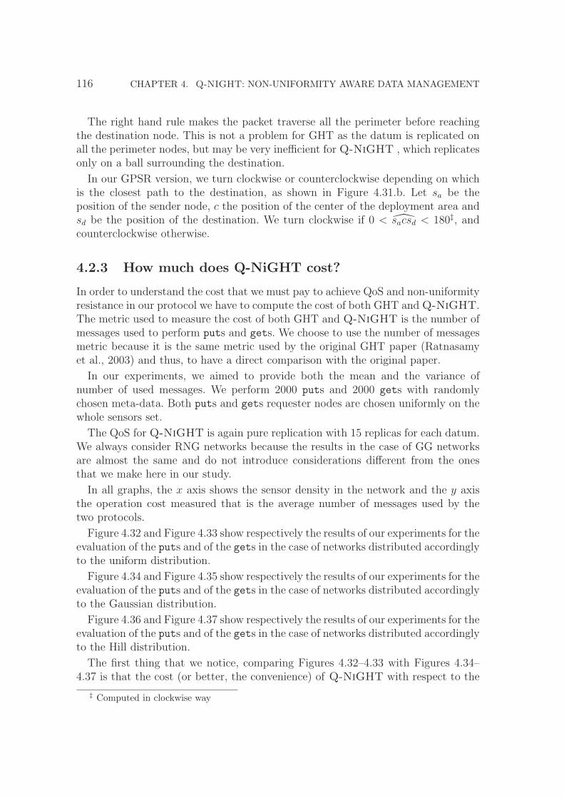
116 CHAPTER 4. Q-NIGHT: NON-UNIFORMITY AWARE DATA MANAGEMENT
The right hand rule makes the packet traverse all the perimeter before reachingthe destination node. This is not a problem for GHT as the datum is replicated onall the perimeter nodes, but may be very inefficient for Q-NiGHT , which replicatesonly on a ball surrounding the destination.
In our GPSR version, we turn clockwise or counterclockwise depending on whichis the closest path to the destination, as shown in Figure 4.31.b. Let sa be theposition of the sender node, c the position of the center of the deployment area andsd be the position of the destination. We turn clockwise if 0 < sacsd < 180‡, andcounterclockwise otherwise.
4.2.3 How much does Q-NiGHT cost?
In order to understand the cost that we must pay to achieve QoS and non-uniformityresistance in our protocol we have to compute the cost of both GHT and Q-NiGHT.The metric used to measure the cost of both GHT and Q-NiGHT is the number ofmessages used to perform puts and gets. We choose to use the number of messagesmetric because it is the same metric used by the original GHT paper (Ratnasamyet al., 2003) and thus, to have a direct comparison with the original paper.
In our experiments, we aimed to provide both the mean and the variance ofnumber of used messages. We perform 2000 puts and 2000 gets with randomlychosen meta-data. Both puts and gets requester nodes are chosen uniformly on thewhole sensors set.
The QoS for Q-NiGHT is again pure replication with 15 replicas for each datum.We always consider RNG networks because the results in the case of GG networksare almost the same and do not introduce considerations different from the onesthat we make here in our study.
In all graphs, the x axis shows the sensor density in the network and the y axisthe operation cost measured that is the average number of messages used by thetwo protocols.
Figure 4.32 and Figure 4.33 show respectively the results of our experiments for theevaluation of the puts and of the gets in the case of networks distributed accordinglyto the uniform distribution.
Figure 4.34 and Figure 4.35 show respectively the results of our experiments for theevaluation of the puts and of the gets in the case of networks distributed accordinglyto the Gaussian distribution.
Figure 4.36 and Figure 4.37 show respectively the results of our experiments for theevaluation of the puts and of the gets in the case of networks distributed accordinglyto the Hill distribution.
The first thing that we notice, comparing Figures 4.32–4.33 with Figures 4.34–4.37 is that the cost (or better, the convenience) of Q-NiGHT with respect to the
‡ Computed in clockwise way

4.2. Q-NIGHT 117
-300
-200
-100
0
100
200
300
400
500
600
4000 6000 8000 10000 12000 14000 16000 18000 20000
Cos
t (m
essa
ges
sent
)
Nodes Number
(a) GHT
-300
-200
-100
0
100
200
300
400
500
600
4000 6000 8000 10000 12000 14000 16000 18000 20000
Cos
t (m
essa
ges
sent
)
Nodes Number
(b) Q-NiGHT
Figure 4.32: Mean and standard deviation of the costs (number of messages) of putwith uniform distribution and RNG planarization.
cost of GHT is different is we consider the uniform case and the non-uniform case.Now, we study this two situations separately.
Uniform case. In the uniform case, shown in Figure 4.32 and in Figure 4.33, showsthat in both Q-NiGHT and GHT have comparable cost in the case of get operation,but in the case of put operation, the performance of Q-NiGHT is better than theperformance of GHT.
The reason of this behavior is that in the case of the put operations, the cost ofGHT is influenced by the use the external perimeters to store data. This is more
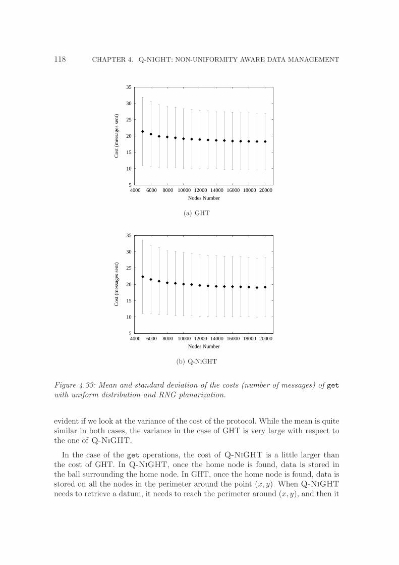
118 CHAPTER 4. Q-NIGHT: NON-UNIFORMITY AWARE DATA MANAGEMENT
5
10
15
20
25
30
35
4000 6000 8000 10000 12000 14000 16000 18000 20000
Cos
t (m
essa
ges
sent
)
Nodes Number
(a) GHT
5
10
15
20
25
30
35
4000 6000 8000 10000 12000 14000 16000 18000 20000
Cos
t (m
essa
ges
sent
)
Nodes Number
(b) Q-NiGHT
Figure 4.33: Mean and standard deviation of the costs (number of messages) of getwith uniform distribution and RNG planarization.
evident if we look at the variance of the cost of the protocol. While the mean is quitesimilar in both cases, the variance in the case of GHT is very large with respect tothe one of Q-NiGHT.
In the case of the get operations, the cost of Q-NiGHT is a little larger thanthe cost of GHT. In Q-NiGHT, once the home node is found, data is stored inthe ball surrounding the home node. In GHT, once the home node is found, data isstored on all the nodes in the perimeter around the point (x, y). When Q-NiGHT
needs to retrieve a datum, it needs to reach the perimeter around (x, y), and then it

4.2. Q-NIGHT 119
0
200
400
600
800
1000
1200
1400
4000 6000 8000 10000 12000 14000 16000 18000 20000
Cos
t (m
essa
ges
sent
)
Nodes Number
(a) GHT
0
200
400
600
800
1000
1200
1400
4000 6000 8000 10000 12000 14000 16000 18000 20000
Cos
t (m
essa
ges
sent
)
Nodes Number
(b) Q-NiGHT
Figure 4.34: Mean and standard deviation of the costs (number of messages) of putwith Gaussian distribution and RNG planarization.
has to be routed around such perimeter until it finds a node in the ball that storesthe datum. In GHT, the query simply needs to reach the perimeter to retrieve thedatum.
Non-uniform case. In the non-uniform case, Q-NiGHT shows better perfor-mances than GHT for both puts and gets.
In Figure 4.34 and in Figure 4.36, we can see the cost of the put operation forboth Gaussian and Hill distributions. In both cases, GHT has a performance that

120 CHAPTER 4. Q-NIGHT: NON-UNIFORMITY AWARE DATA MANAGEMENT
0
5
10
15
20
4000 6000 8000 10000 12000 14000 16000 18000 20000
Cos
t (m
essa
ges
sent
)
Nodes Number
(a) GHT
0
5
10
15
20
4000 6000 8000 10000 12000 14000 16000 18000 20000
Cos
t (m
essa
ges
sent
)
Nodes Number
(b) Q-NiGHT
Figure 4.35: Mean and standard deviation of the costs (number of messages) of getwith Gaussian distribution and RNG planarization.
is 4 to 6 times worst than the case of Q-NiGHT. This behavior is due to the badinteraction between the use of the uniform hashing and the use of the perimetersto store data: the uniform hashing distributes, with the same probability, data indenser and sparser regions, moreover, in sparser regions perimeters are longer thanin denser regions. On the other hand, Q-NiGHT uses the dispersal protocol tostore data and the dispersal protocol guarantees that we need only a small numberof messages to be exchanged to store a datum, once the home node is found.
In Figure 4.35 and in Figure 4.37, we can see the cost of the get operation for

4.2. Q-NIGHT 121
-500
0
500
1000
1500
2000
4000 6000 8000 10000 12000 14000 16000 18000 20000
Cos
t (m
essa
ges
sent
)
Nodes Number
(a) GHT
-500
0
500
1000
1500
2000
4000 6000 8000 10000 12000 14000 16000 18000 20000
Cos
t (m
essa
ges
sent
)
Nodes Number
(b) Q-NiGHT
Figure 4.36: Mean and standard deviation of the costs (number of messages) of putwith Hill distribution and RNG planarization.
both Gaussian and Hill distributions. In both cases, Q-NiGHT has a better per-formance with respect to GHT. This is due to the use of RejectionHash. UsingRejectionHash, Q-NiGHT stores the largest part of data in denser regions. Stor-ing the largest part of data in denser regions has two benefits: (i) the majority ofrequests for data arrives from denser regions too and in turn of it, the requesterstend to be closer to the nodes that store data and (ii) the greedy mode used toroute messages goes though dense regions very fast because nodes are closer. On theother hand, GHT stores data uniformly on all areas (both dense and sparse). When

122 CHAPTER 4. Q-NIGHT: NON-UNIFORMITY AWARE DATA MANAGEMENT
-20
-10
0
10
20
30
40
50
60
4000 6000 8000 10000 12000 14000 16000 18000 20000
Cos
t (m
essa
ges
sent
)
Nodes Number
(a) GHT
-20
-10
0
10
20
30
40
50
60
4000 6000 8000 10000 12000 14000 16000 18000 20000
Cos
t (m
essa
ges
sent
)
Nodes Number
(b) Q-NiGHT
Figure 4.37: Mean and standard deviation of the costs (number of messages) of getwith Hill distribution and RNG planarization.
the nodes need to get a datum, that are more probably inside denser region, theyneed to perform longer paths. The need to perform longer paths is mitigated by theuse of the perimeters that enable a large number of nodes to store a datum and thusthe paths are not much longer than in Q-NiGHT.
This last set of experiments, as well as the others that helped us into the analysis ofGHT and into the design of Q-NiGHT, show how the non-uniformity can influencea widely accepted system such as GHT. Moreover, these experiments show that itis possible to provide new solutions able to deal with non-uniformity and that these
4.3. A Q-NIGHT BASED APPLICATION FOR LOCATION MANAGEMENT 123
solutions do not introduce a large overhead in uniform networks.
4.3 A Q-NiGHT based application for location
management
In this section, we describe an application of Q-NiGHT. In this application, wedeal with another kind of non-uniformity, namely the functional non-uniformity.
In the functional non-uniformity, a network is made up of different kind of nodes.Some of these nodes a simple sensing nodes, while others are nodes that are able toprovide services to the sensing nodes (the servers).
In this scenario, the sensor nodes must be able to locate the servers to use theservices that they provide. To enable the sensors nodes to locate the servers, we useQ-NiGHT. The servers use Q-NiGHT to store their position inside the network.The servers use the ID of the service that they provide as the meta-datum that ishashed to find the point (x, y) where they will store their own position.
When a sensor node needs to use a service, is hashes the service ID and queryperform a get on the point (x, y) = h(ID) to retrieve the position of the server.Then, the sensor contacts the server to use its service.
4.3.1 Heterogeneous wireless sensor networks and locationmanagement
Heterogeneous WSNs are made up of various kinds of nodes. Some nodes are usedas the interface to the physical environment (we will call them sensors). Othernodes act instead as servers, providing services to the other nodes. For instance,in an outdoor intrusion detection application, the sensor are scattered randomly toprovide tracking of possible intruders, while more powerful nodes provide the serviceor connection (e.g., through satellite links) to the end user.
In this section, we define an architecture for enabling efficient discovery of servicesfor the sensors that need them. Servers are organized in two tiers. The first tiercomprises the actual servers (such as the satellite up-link enabled nodes mentionedbefore). Then there is an intermediate server tier (front-end) where some commonnodes (sensor) are chosen for storing the current position of the servers. A sensorthat needs to find a specific service (and hence a server), sends a message to thefront-end of the system and gets back the position of the service. At this point thesensor knows the server position and is able to start using the service needed.
The proposed architecture implements strategies to provide both load distribu-tion and fault-tolerance, as described in the rest of the section. It also makes ex-tensive use of a caching system to speed-up requests and to save energy. The lo-calization/communication infrastructure used as the basis for our architecture isQ-NiGHT.

124 CHAPTER 4. Q-NIGHT: NON-UNIFORMITY AWARE DATA MANAGEMENT
4.3.2 System architecture and operations
In this section we present our two-tier architecture for locating servers efficientlyand in fault tolerant way.
We start by presenting the actors that play important roles in the architecture.These roles are both structural (given by the physical nature of the heterogeneousnetwork) and logical (given the different usage of the same kind of nodes to performdifferent tasks).
Then, we present the operations of service registration and look-up that are pro-vided by the system. The service registration procedure is performed by the serversto communicate their position to the nodes of the network. The look-up procedureis executed by the nodes that require the localization of a service.
4.3.2.1 Actors
There are three categories of nodes in our architecture. The sensors, the servers,and the server locators.
Sensors: the sensors are low power and low cost devices that are equipped withspecial equipment to control their surrounding environment. They also sporta CPU for performing simple computations, and an embedded radio to com-municate with each other.
Servers: the servers are special nodes that are capable to provide some serviceto the sensor nodes. These services range from storage (to keep the senseddata) to perform as gateways between the WSN and the users. Each serverserveri provides one or more services that are identified by a name, for instanceservicej.
Server locators: the server locator nodes are sensor nodes that know the servers,i.e., the services that the servers provide and the server locations in the net-work.
4.3.2.2 Two-tiers servers architecture
The sensors are the clients of the proposed architecture. The architecture per se isformed by two tiers. The back-end of the architecture is made up of the servers thatare able to provide services to the clients. The servers are randomly deployed (as theclients) and need to be localized by the server locators. The server locators form thefront-end of the architecture. The nodes requiring a service query the front-end tohave the position of the the server, or servers, providing that service. Once obtainedthis information, the nodes communicate directly with the back end servers.

4.3. A Q-NIGHT BASED APPLICATION FOR LOCATION MANAGEMENT 125
4.3.2.3 Services localization
Two operations implement service localization: server registration and server dis-covery. The first one is used by the servers to make the server locator aware of theirlocation. The second one is used by the node that needs a service for finding thecorresponding server. These two operations use Q-NiGHT put and get operations.put is used for storing the position of a server and get to retrieve it later.
4.3.2.4 Servers registration
During the network set-up phase the server i determines its position, positioni,and registers it with the server locator nodes. To perform such operation eachserver hashes the name of each of its services and determines the correspondingpoint (x, y). At this time, for each provided service, it performs a put of the pair〈servicej, positioni〉 to the point (x, y) by using Q-NiGHT. The nodes that storethe pair 〈servicej, positioni〉 become the server locator nodes for servicej.
4.3.2.5 Servers discovery
When a node needs servicej, it hashes the service name by using the Q-NiGHT
hash function, finding the point (x, y). Then it performs a get operation of servicej
from point (x, y), i.e., it sends a request toward that point. One of the server locatorsreplies with the position of the server (this operation is called a look-up). In additionto the basic Q-NiGHT get operation, at this time the node caches the position ofthe service/server for future use. It then sends the request for servicej to the server.The use of caches improves the whole look-up process in many ways. First of all,faster replies are provided to those other nodes interested in locating the sameserver whose look-up queries pass through the caching node. Moreover, cachingenables cheaper look-ups because fewer hops can be enough to provide a reply,and lower energy consumption for the server locator nodes is required since theyhave to deal with a lower number of queries. For instance, cached positions increaseinformation retrieval performance in applications such as intrusion detection. In thiscase, messages for a particular server are generated by nodes that are close to eachother and to where the intrusion happens. In this case, spatial locality of caches istaken advantage of.
4.3.2.6 Load distribution and fault-tolerance
By using Q-NiGHT with the strategy described above, our architecture is able tobalance the query load to the locator servers and it is tolerant to location serversfailures. The load balancing property is particularly useful for distributing multiplerequests of the same service to multiple servers that provide it. Fault-tolerancehelps in removing those servers that are no longer available (because of failures or

126 CHAPTER 4. Q-NIGHT: NON-UNIFORMITY AWARE DATA MANAGEMENT
network disconnections) from the list of servers that provide a given service. Thedisappearance of a service/server can be signaled to a server locator by a sensornode who, trying to contact a server, realizes that it is no longer available. Thisfeature of the architecture presents security issues, which we discuss in a separateparagraph at the end of this section.
Load balancing. Query load balancing is provided via multiple server registrations.All the servers that provide a service have the same server locators. This happensbecause the servers share a common service name, say servicej. The server locatorsstore all the coordinates that were provided for each service name. When a requestarrives to a server locator for servicej, the node chooses one of the possible serversaccording to a given strategy (for instance, randomly, or in a a round-robin way,by keeping a pointer to the last server returned and incrementing it modulo thenumber of servers). This method also provides an easy way to increase the numberof servers. When a new server (that provides servicej) enters the network, the serverregisters itself with the server locators and these return the server location as oneof the possible servers for that service.
Fault-tolerance. Fault-tolerance to service outage is obtained as follows. Theservers keep providing their position to the server locators periodically (for instanceeach τ seconds).
In case of service failure, after τ seconds from the last update the server locatorscancel the server position. In the worst case this system provides the cancellation ofa server from server locators after 2τ seconds.
In order to make our protocol completely fault-tolerant we have to remove thecached server positions from the caches of the sensors that stored such information.To this aim, a server position is cached by a sensor for at most τ seconds, afterwhich it is removed from the cache. In case the sensor needs the position of theserver again after τ seconds, it will have to query the server locators again. Finally,if a node queries a server whose entry was in its cache (i.e., τ seconds from its lastquery to a server locator have not passed yet) and the server is no longer available,the server’s (ex) neighbors report an error to the sensor requesting the service. Uponreceiving the error message the node removes the cache entry and performs a get
for a new server for servicej, at the same time communicating to the server locatorsthat the server is unavailable.
Security issues. The capability of sensors to invalidate a service location at a serverlocator makes possible attacks in which the server locators server list are modifiedby malicious (or faulty) nodes.
To address this problem the network user (administrator) can choose betweenthree solutions: (i) the sensors are not allowed to invalidate server locators and/orinvalidation messages are dropped by server locators, (ii) the server locator verifiesthe invalidation querying the server itself to double check about the availability of

4.3. A Q-NIGHT BASED APPLICATION FOR LOCATION MANAGEMENT 127
that server, or (iii) the user provides a cryptography based system to verify theidentity of the message sender and possibly its trust-level. All these solutions areequally powerful to guarantee a minimum level of trust to our architecture. Thechoice of one of them (or any combination of them) depends on the characteristicsof the network (e.g., computational power and energy) as well as the application andenvironmental characteristics (probably, for border monitoring or in the battlefielda level of trust much higher than wildlife monitoring is required).
4.3.3 Experimental results
We have performed experiments for measuring the effectiveness of our service local-ization architecture with respect to the energy cost of querying with and withoutcaches, as well as the cost of the look-up operation.
In the simulation setting, we have considered 5000 WSNs where 5000 sensor nodesare scattered randomly and uniformly in a square area with a side of 1000m. Eachnode has communication range of 30m. Power consumption for transmission is setto 24mW and that for reception is set to 14.4mW as in the EYES sensor proto-types (Havinga et al., 2003). The sensors that perform a look-up operation and thensend a message to the server are uniformly chosen between the deployed sensors.
All the experiments are aimed at showing the effectiveness of the architecture inproviding prompt and energy efficient response to sensor queries. In particular, weshow here that caching is particularly useful in providing a more balanced energyconsumption, and therefore better performance of the network. For this reason, allthe presented experiments are provided with and without nodal cache enabled. Alltests are performed starting from the same seeds to generate the same scenarioswith different architectural parameters. The results we show achieve a statisticalconfidence of 95%, with a precision within 5%.
Figure 4.38, Figure 4.39 and Figure 4.40 depict the cost for a sensor to contactserver locators and servers. In Figure 4.38 the cost is defined as the energy spent bya node to send a packet to the server locators, to get the server location back andthen to perform one communication to the server. In other words, we compute thetotal energy to deliver/receive three packets. In Figure 4.39, the cost is defined onlyas the cost to send a message from a sensor to the server locators and to get theserver location back (that is the energy to send two packets). This provides up witha more detailed idea of how much it costs to the sensor the use of the intermediatetier provided by the sensor locators. Figure 4.40 shows the cumulative cost of thelook-up operation, to have an idea of difference in the growth of the energy cost. Thecumulative cost is computed as follows: the cost of the qth look-up is given by itscost and summed to the cost of all the previous q − 1 look-ups. As mentioned, eachset of experiments is performed with and without the cache mechanism enabled.The network is observed for a time long τ to take into account the maximum usage

128 CHAPTER 4. Q-NIGHT: NON-UNIFORMITY AWARE DATA MANAGEMENT
0.02
0.025
0.03
0.035
0.04
0.045
0.05
0.055
0 100 200 300 400 500 600 700 800 900 1000
Cos
t (J)
Number of queries
Without cachesWith caches
Figure 4.38: Cost for server look-up plus the cost for contacting the servers. Thefigure shows the effectiveness of the caches in our solution. With the growth of thenumber of the queries the cost of the protocol decreases because the nodes cachingthe wanted information grow up.
0.005
0.01
0.015
0.02
0.025
0.03
0.035
0.04
0 100 200 300 400 500 600 700 800 900 1000
Cos
t (J)
Number of queries
Without cachesWith caches
Figure 4.39: Cost for servers look-up operations only. The figure shows in detail theeffectiveness of the caches in our solution (considering that the server contactingoperations cannot be cached in our model).
of the caches before their refresh. In our experiments, τ = 30 minutes i.e., the timethat we need to perform 1000 queries.
Figure 4.38 depicts the cost for each single query in the network with and withoutthe caching enabled. This cost, expressed in Jules, is defined as the sum of the energyspent at each node for propagating the query. This cost is computed considering boththe cost for transmission and reception We observed that when caching is enabledthe cost of the single query decreases with increasing number of queries because the

4.3. A Q-NIGHT BASED APPLICATION FOR LOCATION MANAGEMENT 129
0
5
10
15
20
25
30
35
0 100 200 300 400 500 600 700 800 900 1000
Cos
t (J)
Number of queries
Without cachesWith caches
Figure 4.40: Cumulative cost for servers look-up operations. The cumulative cost forthe qth look-up is given by its cost and summed to the cost of all the previous q − 1look-ups.
caching mechanism becomes more and more effective (more and more nodes havethe location in cache).
Figure 4.39 depicts only the cost of the look-up operation for each single queryin the network with and without the caching enabled on sensors. This cost, as theprevious one, is defined as the sum of the energy spent at each node for propagatingthe query. This case, is analyzed to have a better evaluation of the look-up procedure,that is cached optimized, with respect to the server interaction, that in our scenariodoes not use caches to optimize the sensor-server. Some particular applications canuse caching also between sensors and servers but we chose this situation (the worstcase) in which the interaction with the server is not cached to have a more clearvision of the look-up costs and benefits.
Figure 4.40 depicts the cumulative cost of the look-ups only (sensor-server locatorscommunication and back) without considering the cost for server interaction. In thiscase, we observe that the cost to reach the server locator nodes decreases when thenumber of the queries increases, as expected.
Figure 4.41 presents the (normalized) residual energy level of the server locatorswith and without using caches. The residual energy level of the server locator iscomputed reading the energy level of the server locators before the first refresh ofthe service location by the servers, that restore Q copies of the location, also inthe case in which some server locators run out of energy. The figure shows a highinfluence (36%) of the caches in the energy spent by the server locators in theirfunction.
As shown in the experimental results, the presented architecture provides the lo-calization service in a load-balanced and fault-tolerant way and the caching system

130 CHAPTER 4. Q-NIGHT: NON-UNIFORMITY AWARE DATA MANAGEMENT
1
1.3621
Without cache With cache
Nor
mal
ized
life
time
Figure 4.41: Server locators residual energy level before the server locators refreshstep. The residual energy is normalized to the energy level of the system withoutusing the caches.
enables the nodes that lay in the same region to assist in providing service loca-tion while relieving the service locators of providing the service. Furthermore, theobtained results are encouraging and open up possibilities for further studies andfor the application of this method to problems such as data storage and replication,and similar problems.
4.4 Summary
In this chapter, we have presented our research work in the data management fieldin WSNs.
We presented our contribution, describing Q-NiGHT (Albano et al., 2006a,Albanoet al., 2006b,Albano et al., 2007). Q-NiGHT is a data centric storage system basedon GHT. As well as GHT, Q-NiGHT uses an hash function to provide compute theposition of a datum starting from its mata-data (often called key). Moreover, Q-
NiGHT uses a modified version of the GPSR protocol to route messages inside thenetwork. The key differences between the Q-NiGHT and GHT is in the assumptionmade by the protocol to work. GHT assumes that the network is uniform and thehash function used to find the position of a datum is always the same, independentlyfrom the real distribution of the nodes. On the other hand, Q-NiGHT uses theRejectionHash algorithm distribute data in the network with a distribution thatis an approximation of the network distribution.
Our work focused into the analysis of GHT, throughout simulations and anal-ysis of the experimental results, spotting out its weaknesses in both-uniform andnon-uniform environment. Then, we provided a solution that could overcome the
4.4. SUMMARY 131
problems introduced by a bad initial design and the uniformity assumptions. Q-
NiGHT showed up its flexibility and its ability to work properly in non-uniformlydistributed networks. The extensive simulations performed on Q-NiGHT showedup that all the improvements aimed at providing fair load distribution and QoSfeatures to GHT have a cost and that this cost is not very high if compared to theadvantages in terms of load distribution and memory resources usage.
Finally, we described and evaluated the performances of a possible applicationscenario involving Q-NiGHT. We provide a fault tolerant and load-balanced local-ization system for services in WSNs. In our scenario, we enable a network made upof different types of nodes (some of them are normal sensors and some others areservers) to locate the services provided by the servers and thus to locate the serversin the network. The system provides a simple solution based on a two-tiers serversystem in which some of the sensors act as server-locators storing the position ofthe services and the position of the servers providing them. The server-locators areelected using Q-NiGHT: during the network initialization phase, the servers hashthe name of the services that they provide and store their position in the point re-turned by the hash function. This operation defines a set of server-locators aroundthat point. When a sensor needs a service it simply hashes the service name, sends aquery to the server-locator position and as soon as a replay arrives it begins commu-nicating with the server. This approach is totally generic and can be used to locateany kind of service provided in a simple and reliable way.
In all this chapter, we used Q-NiGHT pretending to know the correct networkdistribution functions, for instance inside the RejectionHash function. This as-sumption is not realistic but it made simpler the description of Q-NiGHT. Obvi-ously, we have also addressed the problem of finding out the distribution of a WSN,which is the central problem for non-uniformly distributed networks. Our researchlead to a system, that we called Stripes. This system is described into the nextchapter.

132 CHAPTER 4. Q-NIGHT: NON-UNIFORMITY AWARE DATA MANAGEMENT
Chapter 5
Stripes: Finding Out Distributions
I’m ten years old. My life is half over and I don’t even know if I’m black with whitestripes or white with black stripes.
- Marty the Zebra (Madagascar, 2005)
Abstract
In the last chapter, we described Q-NiGHT leaving outside our exposition theway in which our system was able to know the network distribution. In thischapter, we present Stripes. Stripes is a suite of protocols and algorithmsthat can be used to find out the network distribution from a fixed number ofsamplings. Moreover, Stripes optimizes energy usage of the network enablingcached information across the network. Stripes is divided in two equallyimportant parts: two network density approximation algorithms, that startingfrom a limited number of samplings rebuild the density of the whole networkand two protocols that are used to sample the density in the network and tospread the computed approximation of the density to the nodes of the networkthat need such density in normal operations.
In the last chapter, we revised Q-NiGHT. Our description of Q-NiGHT intro-duced the RejectionHash algorithm to provide data location during load andstore operations. The RejectionHash algorithm needs to know the distribution ofthe nodes (or an approximation of it). We deliberately postponed the discussion onhow Q-NiGHT is able to know the network distribution.
In this chapter, we move into the description of the protocols that Q-NiGHT
uses to know the distribution of the nodes in the network. These protocols arecalled Stripes and they are proposed to provide an efficient way to reconstruct thesensors’ distribution starting from a few samples. This protocols family is dividedin two equally important parts.

134 CHAPTER 5. STRIPES: FINDING OUT DISTRIBUTIONS
The first part rebuilds an approximation of the density of the network startingfrom few samples using a two steps algorithm: the first step builds a first approxi-mation of the density and the second step performs a refinement step that providesa much better approximation of the network density.
The second part focuses on the dissemination of the sampled densities and of thedensity approximation to all the nodes that need it. We proceed using the followingstrategy: we start from a very simple (and quite inefficient) broadcast algorithm,then we move to an on-demand strategy well suited for networks in which few nodesneed to know the network density and, finally, we provide a very efficient protocolto distribute such information also in networks with a high number of requests.
A note about simulations. In this chapter, as well as in Chapter 4, we make alarge use of simulations to undertand the non-uniformity influence upon networksand to measure the efficience of Stripes. Again, our simulation environment is aself-made simulator that is able to deal with large quantity of nodes and all theexperiments are repeated until we achieve a statistical confidence of 95%, with aprecision within 5%.
Chapter organization. This chapter is organized as follows. Section 5.1 presentsthe motivations behind the Stripes protocols family. Section 5.2 describes howStripes protocols family works and the performance and cost of such protocols.Finally, section 5.3 draws the conclusions of the research work described in thischapter.
5.1 Why do we need Stripes?
Non-uniformity introduces new problems that must be addressed in WNSs research.A non-uniform distribution presents a natural unbalance, for instance in radio in-terferences, and solutions that well fit the needs of a sub area of the network can beuseless in another. Moreover, as we have seen in Chapter 4, non-uniformity can bea great source of load unbalance for data storage inside a network.
On top of all the problems brought by the non-uniformity, there is the problem offinding out the distribution (or an approximation of the distribution) of the networkitself.
This problem is central in the development of non-uniformity resistant solutions.For instance, without such knowledge Q-NiGHT is unable to perform storage loaddistribution in the network throughout the RejectionHash algorithm.
5.2 Stripes
In this section, we present Stripes, which finds out the nodes distribution of aWSNs starting from a fixed number of samples. Stripes, and it is made up two
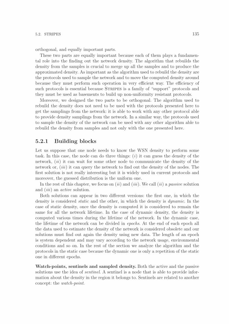
5.2. STRIPES 135
orthogonal, and equally important parts.
These two parts are equally important because each of them plays a fundamen-tal role into the finding out the network density. The algorithm that rebuilds thedensity from the samples is crucial to merge up all the samples and to produce theapproximated density. As important as the algorithm used to rebuild the density arethe protocols used to sample the network and to move the computed density aroundbecause they must perform such operation in very efficient way. The efficiency ofsuch protocols is essential because Stripes is a family of “support” protocols andthey must be used as basements to build up non-uniformity resistant protocols.
Moreover, we designed the two parts to be orthogonal. The algorithm used torebuild the density does not need to be used with the protocols presented here toget the samplings from the network: it is able to work with any other protocol ableto provide density samplings from the network. In a similar way, the protocols usedto sample the density of the network can be used with any other algorithm able torebuild the density from samples and not only with the one presented here.
5.2.1 Building blocks
Let us suppose that one node needs to know the WSN density to perform sometask. In this case, the node can do three things: (i) it can guess the density of thenetwork, (ii) it can wait for some other node to communicate the density of thenetwork or, (iii) it can query the network to find out the density of the nodes. Thefirst solution is not really interesting but it is widely used in current protocols andmoreover, the guessed distribution is the uniform one.
In the rest of this chapter, we focus on (ii) and (iii). We call (ii) a passive solutionand (iii) an active solution.
Both solutions can appear in two different versions: the first one, in which thedensity is considered static and the other, in which the density is dynamic. In thecase of static density, once the density is computed it is considered to remain thesame for all the network lifetime. In the case of dynamic density, the density iscomputed various times during the lifetime of the network. In the dynamic case,the lifetime of the network can be divided in epochs. At the end of each epoch allthe data used to estimate the density of the network is considered obsolete and oursolutions must find out again the density using new data. The length of an epochis system dependent and may vary according to the network usage, environmentalconditions and so on. In the rest of the section we analyze the algorithm and theprotocols in the static case because the dynamic one is only a repetition of the staticone in different epochs.
Watch-points, sentinels and sampled density. Both the active and the passivesolutions use the idea of sentinel. A sentinel is a node that is able to provide infor-mation about the density in the region it belongs to. Sentinels are related to anotherconcept: the watch-point.
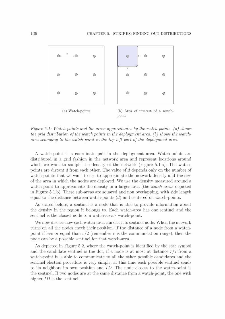
136 CHAPTER 5. STRIPES: FINDING OUT DISTRIBUTIONS
d
(a) Watch-points
d
d
(b) Area of interest of a watch-point
Figure 5.1: Watch-points and the areas approximates by the watch points. (a) showsthe grid distribution of the watch points in the deployment area. (b) shows the watch-area belonging to the watch-point in the top left part of the deployment area.
A watch-point is a coordinate pair in the deployment area. Watch-points aredistributed in a grid fashion in the network area and represent locations aroundwhich we want to sample the density of the network (Figure 5.1.a). The watch-points are distant d from each other. The value of d depends only on the number ofwatch-points that we want to use to approximate the network density and the sizeof the area in which the nodes are deployed. We use the density measured around awatch-point to approximate the density in a larger area (the watch-areas depictedin Figure 5.1.b). These sub-areas are squared and non overlapping, with side lengthequal to the distance between watch-points (d) and centered on watch-points.
As stated before, a sentinel is a node that is able to provide information aboutthe density in the region it belongs to. Each watch-area has one sentinel and thesentinel is the closest node to a watch-area’s watch-point.
We now discuss how each watch-area can elect its sentinel node. When the networkturns on all the nodes check their position. If the distance of a node from a watch-point if less or equal than r/2 (remember r is the communication range), then thenode can be a possible sentinel for that watch-area.
As depicted in Figure 5.2, where the watch-point is identified by the star symboland the candidate sentinel is the dot, if a node is at most at distance r/2 from awatch-point it is able to communicate to all the other possible candidates and thesentinel election procedure is very simple: at this time each possible sentinel sendsto its neighbors its own position and ID. The node closest to the watch-point isthe sentinel. If two nodes are at the same distance from a watch-point, the one withhigher ID is the sentinel.

5.2. STRIPES 137
r r/2
Figure 5.2: Sentinel and watch-point distance relation with respect to the communi-cation range r.
Once the sentinel node is elected, the sentinel node counts the nodes inside itscommunication range. The number of the nodes inside the sentinel’s communicationrange is the reported density for the corresponding watch-point.
In the case in which no node close is as close as r/2 to a watch-point, the watch-point is said to be unguarded and the reported density for its watch-area will be0.
There is an important relation between d and r: it is must be always true that
d ≥ 3r
this is because the sentinel counts how many nodes belongs to the circle or radius rcentered on the sentinel itself. Since a sentinel can be as far as r/2 from its watch-point, having d < 3r can bring nodes from different areas in the sentinel circle.
Thus, if we want a sentinel to report only the nodes inside its own watch-area,the watch-area must be greater than the maximum possible distance from a watch-point, at which a sentinel is able to find, and count, nodes. This implies that thewatch-area side must be greater than 2(r + r/2) = 2(3r/2) = 3r.
Figure 5.3 shows the relationship between d and r. From the picture it is clearthat a smaller d implies that on sentinel can use, to estimate the density, nodes thatbelong to other sentinels and/or watch-points.
5.2.2 Moving density around: broadcast, Stripes and Fat-Stripes
In this section, we discuss how sampled densities from watch-points can be deliveredto other nodes of the network.

138 CHAPTER 5. STRIPES: FINDING OUT DISTRIBUTIONS
rr r/2 r/2
d
Figure 5.3: Relation between d and r. d must be greater or equal than 3r to guaranteethat a sentinel reports only the nodes inside its own watch-area.
As stated before, there are two different solutions to address the problem of in-forming the nodes inside the network of its distribution: the passive solution andthe active solution.
In passive solution, each sentinel broadcasts the network density that it foundout in its watch-area to all the nodes inside the network. In the active solution, thenodes that need to know the network density query the sentinels to know the densityinside each watch-area.
In this section we revise this two solutions. Moreover, for the active solution, weprovide two different protocols: Stripes and Fat-Stripes. Stripes is the firstimplementation of the active solution that uses caches to optimize the energy usage.Fat-Stripes is an optimization of Stripes. Fat-Stripes uses the caches in amore aggressive way to save even more energy.
5.2.2.1 Passive solution
In the passive solution, a network finds out its own density during a bootstrap phase.
When the network turns on, all the nodes check their position and for each watch-area sentinel are elected. Once the sentinels election procedure is done and after thateach sentinel has collected the number of nodes to be reported the sentinels broadcastto every node in the network the pair 〈watch − pointxy, number of nodes〉.
In the case of unguarded watch-areas, no sentinel is elected and no message isbroadcasted. Thus, the absence of messages from a watch-point is interpreted as zeroin the corresponding watch-area. To ensure a correct termination of the network setup operation, a time out is used in order to prevent that nodes wait for a densityvalue coming from a particular watch-point forever.

5.2. STRIPES 139
After the reception of the data from the sentinels and after the time out expired,all the nodes start to rebuild the density of the network according to the algorithmthat will be described in Section 5.2.3.
The cost of the passive protocol (in terms of energy used to communicate thedensity) is given by the cost of k broadcasts operations, where k is the number ofsentinels inside the network.
5.2.2.2 Active solution (Stripes)
On the other hand, the active solutions, each node that needs to know the networkdensity queries the network to have such value. The query operation is performedsending a message to a watch-point. The sent message will reach the closest pointto the watch-point, that is the sentinel. The sentinel, in turn of the reception of thequery sends back the sampled density to the requester.
In the active protocol, there are two different cases to consider: (i) the node thatqueries the network to know the density is the first one attempting to do so and (ii)the node that do so it is not the first one. We consider the two cases.
A node that needs to know the distribution of the sensors in the network, sendsa message, using GPSR (Karp and Kung, 2000), to each watch-point. The GPSRprotocol finds the closest node to the watch-point (that must be a sentinel if it iscloser than r/2 to the watch-point). In response to the query, the sentinel sends backto the querier the pair 〈watch − pointxy, number of nodes〉.
If the closest node found by the GPSR perimeter mode, to the watch-point ismuch far than r/2, it sends back the pair 〈watch − pointxy, 0〉.
After the reception of the data from the sentinels the node starts to rebuild thedensity of the network as described in Section 5.2.3.
In order to improve subsequent queries from nodes traversing the same path,on the way back to the requester, the pair 〈watch − pointxy, number of nodes〉 iscached on all the nodes belonging to the path, creating cache stripes across thenetwork (a stripe for each watch-point).
Consider now what happens when a node queries the watch-point after manyothers have done so. As soon as the query message reaches a node belonging to acache stripe in a path belonging to a previous query, a reply is sent directly by thenode belonging to the stripe without needing to reach the watch-point. If a nodebelonging to a stripe needs to know the density of the network, it simply queries thewatch-points for which it has no cached data.
The idea behind the stripes is that, after some initial queries, a node is able tofind all the data it needs at a few hops of distance from itself. Due to the presenceof cache stripes we call this protocol Stripes.
In order to understand the if our intuition is correct and to measure the realcost of Stripes we have performed detailed simulations of it. To measure the cost

140 CHAPTER 5. STRIPES: FINDING OUT DISTRIBUTIONS
0
50
100
150
200
250
300
0 500 1000 1500 2000 2500 3000 3500 4000 4500 5000
Cos
t (J)
Queries
9 Watch-points16 Watch-points25 Watch-points36 Watch-points
(a) Uniform
0
100
200
300
400
500
600
700
800
0 500 1000 1500 2000 2500 3000 3500 4000 4500 5000
Cos
t (J)
Queries
9 Watch-points16 Watch-points25 Watch-points36 Watch-points
(b) Gaussian
0
50
100
150
200
250
300
350
400
450
500
0 500 1000 1500 2000 2500 3000 3500 4000 4500 5000
Cos
t (J)
Queries
9 Watch-points16 Watch-points25 Watch-points36 Watch-points
(c) Hill
Figure 5.4: Cumulative cost of the Stripes protocol.

5.2. STRIPES 141
we compute the energy (in Joules) spent by the network to collect data from thewatch-points.
The simulations have the following parameters. We simulate the deployment of5000 nodes in a squared area of size 1000m×1000m. Each node has a communicationrange of 30m. We use 9, 16, 25 and 36 watch-points placed in a squared grid fashion.We distribute nodes using uniform, Gaussian (with σ = 1 and average in the centerof the deployment area) and Hill distributions (stretched to fit the 1000m × 1000marea). The transmission power is set to 24mW and the receive power to 14.4mW asin (Havinga et al., 2003). The idle power is set to 0 because we are interested onlyin the raw cost of our protocols, without considering the energy spent in idle state.For each test we generate 5000 requests to find the density: a request for each nodeof the network. The order in which the nodes are elected to send the requests is anuniform permutation of the whole nodes set.
Figure 5.4.a, Figure 5.4.b and Figure 5.4.c show the total energy spent by thenetwork. These values are presented in a cumulative way: the cost of the qth queryis given by its cost added to the cost of all the previous q − 1 queries.
As we can expect, the total cost of the protocol increases with the number ofqueries, but the curve is less step as the number of queries increases. This is dueto cache effect on the length of the routes that must be traversed to find the valueto be returned. The first time that a query is performed it must be routed as closeas possible to the watch-point. The second time a request can stop before reachingthe watch-point because the request has hit a cached density value on a node thatis part of a stripe. This effect increases with the number of queries because moreand more nodes are part of the cache. Moreover, the total cost increases with thenumber of watch-points because more queries must be performed in order to get allthe densities from all the watch-areas.
5.2.2.3 A better active solution (Fat-Stripes)
The Stripes experimental results show that the use of caches is able to reduce thecost of the queries to get the densities from all the watch-areas.
However, we can observe that cache stripes produced by the Stripes protocolare “thin” stripes. As depicted in Figure 5.5.a, the only nodes that belong to thestripes are the one used as relay nodes by the GPSR protocol on the way back tothe node that required the density.
A major problem with this approach is that all the nodes that do not activelycooperate to move data, but still receive the packets spend their energy into thereception of the message without having any benefit.
This is the key observation for an improvement of Stripes called Fat-Stripes
that works in the same way of Stripes, with only one difference: the nodes thatpassively receive a 〈watch − pointxy, number of nodes〉 packet and that are notinvolved actively into the communication cache the datum too.

142 CHAPTER 5. STRIPES: FINDING OUT DISTRIBUTIONS
(a) Stripes (b) Fat-Stripes
Figure 5.5: Nodes that cache the pair 〈watch − pointxy, number of nodes〉 on theway back of a query.
As depicted in Figure 5.5.b, the cache stripes produced by the Fat-Stripes
protocol are now larger, including all the passive receivers ant the correspondingcache stripes have become “fat”. The aim of this little improvement is to increasethe number of nodes that do not need to communicate to query the network.
In order to measure the effectiveness of this improvement, we simulated again thesame networks of Section 5.2.2.2.
As did for Stripes, or each test we generate 5000 requests to find the density: arequest for each node of the network. The order in which the nodes are elected tosend the requests is an uniform permutation of the whole nodes set.
Figure 5.6.a, Figure 5.6.b and Figure 5.6.c show the total energy spent by thenetwork. These values are presented in a cumulative way: the cost of the qth queryis given by its cost and summed to the cost of all the previous q − 1 queries.
The total cost of the protocol increases in a slower way with respect the Stripes
protocol. This is due to the presence of larger stripes. Larger stripes contain nodesthat do not need to communicate to know the density of the network because thisknowledge derives from listening packets that carry that information.
The performance improvement of Fat-Stripes over Stripes is very high: In theuniform distribution case Fat-Stripes uses less than the 13% of the energy usedby Stripes, in the Gaussian distribution case Fat-Stripes uses less than the 6%of the energy used by Stripes and in the Hill distribution case Fat-Stripes usesless than the 10% of the energy used by Stripes. The advantage of Fat-Stripes
over Stripes is more evident in non-uniform distributions because in non-uniformdistributions we have areas in which the nodes are much closer to each other. The

5.2. STRIPES 143
0
5
10
15
20
25
30
35
40
45
0 500 1000 1500 2000 2500 3000 3500 4000 4500 5000
Cos
t (J)
Queries
9 Watch-points16 Watch-points25 Watch-points36 Watch-points
(a) Uniform
0
5
10
15
20
25
30
35
40
45
0 500 1000 1500 2000 2500 3000 3500 4000 4500 5000
Cos
t (J)
Queries
9 Watch-points16 Watch-points25 Watch-points36 Watch-points
(b) Gaussian
0
5
10
15
20
25
30
35
40
45
0 500 1000 1500 2000 2500 3000 3500 4000 4500 5000
Cos
t (J)
Queries
9 Watch-points16 Watch-points25 Watch-points36 Watch-points
(c) Hill
Figure 5.6: Cumulative cost of the Fat-Stripes protocol.

144 CHAPTER 5. STRIPES: FINDING OUT DISTRIBUTIONS
closer nodes increase the effect of the “fat” stripes because a lot of nodes receive andcache data without being active relays in the communication. As well as Q-NiGHT,Fat-Stripes is able to use the non-uniformity of the network as an advantage.
From these results it is evident that the little modification in nodes behavior in-troduced by the Fat-Stripes protocol with respect to Stripes, brings a very bigimprovement in the protocol’s communications cost without increasing the complex-ity of the original Stripes protocol.
5.2.2.4 Stripes vs. Fat-Stripes
The performance advantage of Fat-Stripes with respect to Stripes is very evidentand it was discussed in Section 5.2.2.3. Fat-Stripes overcomes Stripes in everycases, requiring a very small number of messages, due to the use of caches.
On the other hand, the use of the caches represents an increase in the memoryusage of the nodes. Every node that receives a sampling message stores the sample,also if the node will never use it. It is even true that the memory usage to store thesamplings is very limited and with a constan upper bound given by the number ofthe watch-points times the size used to represent the value of a sampling.
From the viewpoint of a network designer, the size used to used to represent thevalue of a sampling is upper bounded by the number of the nodes inside the network.For instance, if the maximum number of the nodes that a user can deploy is as largeas N , the bits needed to store the value of a single sampling can be as large aslog(N) + 1: log(N) bits are effectively used to store the cache value and the extrabit is a flag used to tell if the cache line is a valid value (i.e., a cached sampling) ora missing value (i.e., a value that is unknown and that must be queried). The sameflag bit is used to invalidate cache lines in the of dynamic densities at the end ofeach epoch.
Thus, if we have K watch-points points, the maximum size, in bits, used for thecached samples is K log(N) + K. For instance, in the case of a network made upof 100000 nodes and with 25 watch-points, the size of the cache is 450 bits (i.e., 57bytes).
5.2.3 Density rebuilding algorithm
In both passive and active protocols, once a node gets the number of nodes at eachwatch-point, it must rebuild the density of the network, creating a bucket densitystructure in which each bucket represents a watch-area.
Here, we propose a simple algorithm to rebuild density. The algorithm acts in twosteps: the first step rebuilds the network density as the the number of nodes reportedin each watch-area by the sentinels over the total number of nodes reported by allthe sentinels and the second step adjusts such values performing a weighted meanof each watch-area with the neighbor watch-areas.

5.2. STRIPES 145
In the first step (the pseudo-code is presented in Algorithm 3), we reconstruct thedensity of each bucket as the fraction of the reported nodes in that bucket over thetotal number of nodes reported.
Algorithm 3 RebuildDensity(W )
Require: The set W of messages from watch-points/sentinels.Ensure: The set D of rebuilt densities.
tot ← 0for all wi,j ∈ W do
tot ← tot + wi,j.nodesend forfor all di,j ∈ D ∧ wi,j ∈ W do
di,j ← wi,j/totend for
Algorithm 3 acts as following. The number of nodes reported in each watch-areawi,j are summed up and stored into tot. Then, the approximated density of eachwatch-area di,j is computed as the fraction of the nodes reported in such area wi,j
with the total number of nodes tot. In practice, the algorithm assumes that thetotal number of the nodes inside the whole network is only the total number of thereported nodes and that the number of nodes in each watch-area is the only the onereported by each sentinel.
This approximation can bring to two pathological situations: (i) false zeroes and(ii) over reported nodes. The false zeroes are reported by areas that have very sparsenodes, or the nodes are not deployed near the watch-point (for instance in a corner),and the possible sentinels can be too far from their watch-point and then a zero isreported when nodes are present. Over reported nodes refers to the opposite problem.In the case of the over reported nodes, we have that the majority of the nodes in awatch-area are concentrated near a watch-point and an extra-large number of nodesis reported.
Figure 5.7 depicts the problem of false zeroes. If we consider the watch-point inthe shaded watch-area, it reports only few (or zero) nodes due to the fact that thewatch-point is located in a low density part of the watch-area. This value is notindicative of the real quantity of nodes in the watch-area because the majority ofthe nodes are located near the left border of the watch-area.
To overcome these two problems, we perform the second step. In the second step(the pseudo-code is presented in Algorithm 4), we apply a smoothing step to thedensity computed by the RebuildDensity algorithm: the computed density foreach watch area is substituted by the weighted average of watch-area density itselfwith the computed densities of its neighbors watch-areas.

146 CHAPTER 5. STRIPES: FINDING OUT DISTRIBUTIONS
Figure 5.7: False zeroes problem.
Algorithm 4 SmoothDensity(D)
Require: The set D of densities.Ensure: The set D′ of smoothed densities.
for all di,j ∈ D ∧ d′i,j ∈ D′ do
d′i,j ← weighted mean of di,j and its neighbors watch − areas
end for
Algorithm 4 works as follows. For each computed density di,j, the algorithm com-putes the weighted mean of di,j with the ones computed into the 4 neighbor watch-areas (i.e., di+1,j, di−1,j,di,j+1 and di,j−1). For the areas on the border the 3 neighborwatch-areas and for the ones in the corners the 2 neighbor watch-areas. In theweighted mean computation, the value di,j is multiplied by the number of neighborswatch-areas used to compute the average.
We evaluate the RebuildDensity and of the SmoothDensity algorithms usingsimulations.
The simulations have the same parameters of the simulations presented in Sec-tion 5.2.2.2.
We measure the “fit” of the approximation computing the error in the computeddensity with respect to the real one. To compute the error, for each watch-area,we compute the square of the difference between the real percentage of nodes inthe watch-area and the one computed by our protocol. The error is defined as theaverage of the squared of the differences computed for all the watch-areas composingthe network.
The results, depicted in Figure 5.8, show, for each one of the analyzed distribu-tions, the average of the errors computed for each simulation. We present the averageerror for both the Algorithm 3 alone and Algorithm 3 and Algorithm 4 together.

5.2. STRIPES 147
0
0.0005
0.001
0.0015
0.002
0.0025
0.003
0.0035
0.004
493625169
Err
or
Watchpoints
uniformnormal
hill
(a) Error after the execution of the RebuildDensity al-gorithm
0
0.0005
0.001
0.0015
0.002
0.0025
0.003
0.0035
493625169
Err
or
Watchpoints
uniformnormal
hill
(b) Error after the execution of the SmoothDensity al-gorithm
Figure 5.8: Average error in approximation algorithm. (a) is the error introduced bythe in the RebuildDensity algorithm and (b) is the error after the smoothing stepperformed by the SmoothDensity algorithm.
The smoothing step, performed by Algorithm 4, is always effective and lowers theerror in all the cases. However, its effect is more evident when the protocol uses fewwatch-points, because a lesser number of watch-points sample very few nodes withrespect to the real number of nodes into the network and the probability to reportfalse zeroes or over reported nodes is larger. In all cases, the error is very low. Asthe number of watch-points increase, the error decreases, and the smoothing step is,

148 CHAPTER 5. STRIPES: FINDING OUT DISTRIBUTIONS
in turn, less effective, as expected.
From an implementation point of view, the two proposed algorithms are verysimple and can be easily implemented on a sensor. Both algorithms use only sum,multiplication and division operations that are usually provided by current proces-sors hardware.
5.2.4 Comparative cost of active and passive protocols
In this section, we compare the costs of the broadcast, the Stripes and the Fat-
Stripes protocols to complete our evaluation of the proposal.
Our comparative evaluation is divided into two parts. The first part provides ananalytical study of the protocol cost and the second one is an experimental studyof such costs.
In the analytical study of the cost, we model both the broadcast and a simpli-fied version of the Stripes protocol (without using caches) to have a comparativeorder of size between a generic passive protocol and a generic active protocol. Theanalytical study of the cost measures the cost of the protocols in terms of sentmessages.
In the experimental study of the cost, we perform simulations of all the protocolsand we compare them to study the behavior of the protocols with uniform, Gaussianand Hill distributions. The experimental study of the cost measures the cost of theprotocols in terms of energy used by the network.
5.2.4.1 Analytical study of the cost
Before going into detailed simulations, we want to explore this issue theoretically. Weassume a simplified setting. The first assumption is related to the fact that we intendto study networks that are deployed using a fair distribution. The characteristics ofa fair distribution are drawn into the following definition:
Definition 5.2.1 (Fair distribution). A node distribution f is fair if and only if
1. ∀Ai s.t. Ai ∈ domain of f and Ai is non null,∫
Aif(x, y)dxdy > 0.
2. The diameter of the deployed network is close to√
n, where n is the totalnumber of deployed nodes.
¤
The first part of the definition states that the nodes could be distributed in allthe deployment area. The second part states that the distribution function of thenetwork is not too step.

5.2. STRIPES 149
For instance, the uniform distribution is a good example of fair distribution, butthe Gaussian distribution is not.
The study takes into account, for the passive solution, a “good” broadcasts al-gorithm, that is one that forward the data only once for each node (with a totalnumber of exchanged messages comparable to n, the size of the network), and forthe active solution does not take into account the effect of the cache stripes.
Let us suppose that in the passive solution all the k sentinels broadcast their data.The total cost of this operation is
Cp = kn. (5.2.1)
Equation (5.2.1) shows that the cost of the passive protocol is proportional to thecost of the k broadcasts needed for each sentinel value.
In a fair distribution, the cost of the active solution, for each request, is
Csinglea = 2k
√n. (5.2.2)
Equation (5.2.2) shows that the cost of the active protocol for each request isgiven by the cost of sending a message to each sentinel that, in the worst case, is atthe largest distance in the network (its diameter) times the number of sentinels. Wemust multiply this value by two because, for each query, we need a reply.
The total cost of the active solution depends on the number Q of queries that areperformed
Ca =
Q∑
i=1
Csinglea = 2kQ
√n. (5.2.3)
Equation (5.2.3) shows the total amount of messages sent considering that thenetwork needs to query Q times the sentinels to know the density.
In the static case, to measure the convenience of a protocol with respect to theother, we must find when
Cp < Ca
kn < 2kQ√
n.
The previous relation is satisfied when
Q >
√n
2(5.2.4)
Equation (5.2.4) shows that, in the static case, the passive solution is more con-venient than the active one if the number of queries that the protocol will need islarger than
√n/2.

150 CHAPTER 5. STRIPES: FINDING OUT DISTRIBUTIONS
epoch 1 epoch 2 epoch 3 ....
Passive Cost
Active Cost
Figure 5.9: The convenience of the active protocol with respect to the passive protocolin the dynamic case.
In the dynamic case, this relation is not valid for all the network lifetime, but itdoes hold for each epoch. In this case, we can find a number of queries Q′, for eachepoch, such that the active protocol is always convenient with respect to the passiveone.
As depicted in Figure 5.9, in the dynamic case the cost of the passive protocolincreases at each epoch of the same quantity kn creating a steps-like graph. Onthe other hand, the active protocol increases constantly with time, independentlyfrom the epochs. Thus, in the dynamic case, if the number of queries performed bythe protocol, Q′, in each epoch is less than
√n/2, the cost of the active protocol is
always smaller than the cost of the passive protocol.
5.2.4.2 Experimental study of the cost
This last set of results compares the cost of the active protocols with the costof the passive one. Our aim is to spot out the differences between the protocolspresented and to understand the reasons of these differences. Moreover, we comparethe experimental results with the analytical ones to understand better how thecaches can influence the behavior of both Stripes and Fat-Stripes.
We expect a big difference between the experimental results and the analyticalones due to use of real distributions and caches. Real distributions can be not asfair as assumed in the theoretical model and caches play an important role in thecost of the protocols.
In order to compare the tree protocols, we performed simulations with the sameparameters used in Section 5.2.2.2.
5.2. STRIPES 151
Also in this experiment, for each test we generate 5000 requests to find the density:a request for each node of the network. The order in which the nodes are elected tosend the requests is an uniform permutation of the whole nodes set.
The results that we present in Figures 5.10–5.12 are structured as follows: for eachdistribution (uniform, Gaussian and Hill) and for each number of watch-points, wecompare the costs, in terms of energy spent by the passive solution, by Stripes andby Fat-Stripes.
On the x axis of the charts, we have the number queries and on the y axis, wehave the energy spent by the network. The graph of the energy is presented in acumulative way: the cost of the qth query is given by its cost added to the cost ofall the previous q − 1 queries. The cost of the passive solution is independent fromthe number of the performed queries, thus it is represented by an horizontal line.
Figures 5.10.(a–d) show the comparative results in the case of uniform distributionfor different numbers of watch-points. In the case of uniform distributions, we canobserve that the total cost of the Stripes protocol (after 5000 queries) is twice thecost of the passive one because we have that for each point we need to pay for thequery and for the replay. The effect of caches is very evident here. Equation (5.2.4)suggests that the limit of convenience in the use of Stripes protocol is
√n/2, that
for n = 5000, is approximatively 35. In our experiments, this value is raised to valuesnear 1000. The cache effect influenced the protocol efficiency by a factor of 28.
The effect of caches is even more evident in the Fat-Stripes protocol. The pro-tocol cost is lower than the cost of the other two protocols. This is due to the useof large cache stripes. In the passive protocol, each node sends the sampled densityone time and all the nodes can receive it multiple times, each time paying the costof receiving a message. The Stripes protocol caches values only on relay nodes: allthe nodes that are not in the relay path still spend their energy receiving a messagewithout the benefit of caching useful information. The Fat-Stripes protocol cachesvalues in both relay nodes and nodes that passively received replay messages: theselast nodes apply the principle that if they spent energy in receiving a message, it isconvenient to cache information brought by the message, because such knowledgecould be used in the future.
Figures 5.11.(a–d) show the comparative results in the case of Gaussian distribu-tion for different numbers of watch-points. In the case of Gaussian distributions, wecan observe that the total cost of the Stripes protocol (after 5000 queries) is morethan the double of the passive one. This is due to the fact that Gaussian distribu-tion is not as fair as uniform distribution. Some watch-points are in sparser regionsof the network (near the borders) and then they have no sentinels. In the case inwhich the watch-point is in a border region of the network, GPSR must route thequery all along the external perimeter of the network. This fact increases the totalcost of the protocol that grows faster than in the uniform case. Also in this case,in despite of the fact of the distribution is not fair, cache stripes do an excellentjob. The Stripes protocol is better than passive one still until 250–300 queries are

152 CHAPTER 5. STRIPES: FINDING OUT DISTRIBUTIONS
performed, that is a factor 7 with respect to the theoretical result. As in the uniformcase, the Fat-Stripes cost never grows to the level of the passive protocol nor tothe level of the Stripes protocol.
In the case of Gaussian distribution, the external perimeter affects negativelythe cost of Stripes. On the other hand in Fat-Stripes, such long perimetersbecomes an advantage because a lot of sensors, belonging to the external perimeterof the network, become caches for the replays to all the queries directed outside thenetwork: less nodes will need to query the network for the density and a cache ring,around the external perimeter, is able to cache replays for more watch-points.
Figures 5.12.(a–d) show the comparative results in the case of Hill distributionfor different numbers of watch-points. This case is in middle between the uniformand the Gaussian case. This is due to the fact that Hill distribution is fairer thanthe Gaussian one, but less fair than the uniform one. With the Hill distributioncache stripes work better than Gaussian but worse than uniform. The active pro-tocol advantage still until 600–700 queries are performed, that is a factor 17 withrespect to the theoretical result. As in the uniform and Gaussian cases, the Fat-
Stripes cost never grows to the level of the passive protocol nor to the level of theStripes protocol. In this case, the advantage of external perimeters is less evidentin Fat-Stripes protocol because the distribution is more fair than the Gaussiandistribution.

5.2.ST
RIP
ES
153
0
10
20
30
40
50
60
70
80
0 500 1000 1500 2000 2500 3000 3500 4000 4500 5000
Cos
t (J)
Queries
StripesFat-Stripes
Passive
(a) 9 watch-points
0
20
40
60
80
100
120
140
0 500 1000 1500 2000 2500 3000 3500 4000 4500 5000
Cos
t (J)
Queries
StripesFat-Stripes
Passive
(b) 16 watch-points
0
20
40
60
80
100
120
140
160
180
200
0 500 1000 1500 2000 2500 3000 3500 4000 4500 5000
Cos
t (J)
Queries
StripesFat-Stripes
Passive
(c) 25 watch-points
0
50
100
150
200
250
300
0 500 1000 1500 2000 2500 3000 3500 4000 4500 5000
Cos
t (J)
Queries
StripesFat-Stripes
Passive
(d) 36 watch-points
Figure 5.10: Comparative cost of the protocols (uniform case).

154C
HA
PT
ER
5.ST
RIP
ES:FIN
DIN
GO
UT
DIS
TR
IBU
TIO
NS
0
20
40
60
80
100
120
140
160
180
200
0 500 1000 1500 2000 2500 3000 3500 4000 4500 5000
Cos
t (J)
Queries
StripesFat-Stripes
Passive
(a) 9 watch-points
0
50
100
150
200
250
300
350
0 500 1000 1500 2000 2500 3000 3500 4000 4500 5000
Cos
t (J)
Queries
StripesFat-Stripes
Passive
(b) 16 watch-points
0
100
200
300
400
500
600
0 500 1000 1500 2000 2500 3000 3500 4000 4500 5000
Cos
t (J)
Queries
StripesFat-Stripes
Passive
(c) 25 watch-points
0
100
200
300
400
500
600
700
800
0 500 1000 1500 2000 2500 3000 3500 4000 4500 5000
Cos
t (J)
Queries
StripesFat-Stripes
Passive
(d) 36 watch-points
Figure 5.11: Comparative cost of the protocols (Gaussian case).

5.2.ST
RIP
ES
155
0
20
40
60
80
100
120
0 500 1000 1500 2000 2500 3000 3500 4000 4500 5000
Cos
t (J)
Queries
StripesFat-Stripes
Passive
(a) 9 watch-points
0
50
100
150
200
250
0 500 1000 1500 2000 2500 3000 3500 4000 4500 5000
Cos
t (J)
Queries
StripesFat-Stripes
Passive
(b) 16 watch-points
0
50
100
150
200
250
300
350
0 500 1000 1500 2000 2500 3000 3500 4000 4500 5000
Cos
t (J)
Queries
StripesFat-Stripes
Passive
(c) 25 watch-points
0
50
100
150
200
250
300
350
400
450
500
0 500 1000 1500 2000 2500 3000 3500 4000 4500 5000
Cos
t (J)
Queries
StripesFat-Stripes
Passive
(d) 36 watch-points
Figure 5.12: Comparative cost of the protocols (hill case).

156 CHAPTER 5. STRIPES: FINDING OUT DISTRIBUTIONS
5.3 Summary
In this chapter, we focused in finding out the distribution of a network of sensors.
Finding out the density of a network is the most important problem in non-uniformnetworks. When we drop the uniformity assumption and we want to deal with non-uniformly distributed networks, we must find new protocols and systems able toprovide the intended services independently from the distribution of the network.Some of these systems, such as Q-NiGHT, need to compute the distribution of thenetwork to provide fair load distribution a good resources usage.
In this chapter, we studied both the problem of density reconstruction startingfrom a predefined number of samples, providing a simple but effective algorithm(and its refinement step too), and the protocols to enable the sensors of the networkto compute the distribution of the nodes.
For this second point, we started from a very simple timed-out broadcast protocolthat spread the sampled density to all the nodes of the network. Then we movedto a more sophisticated density-on-demand protocol, namely Stripes, that is veryefficient in the case of a low traffic network but it is not so good in high trafficnetworks.
To overcome the problem of Stripes with high traffic networks, we provided anew protocol (Fat-Stripes) that, using an opportunistic caching strategy, is ableto provide density-on-demand in a very efficient way in all traffic conditions.

Conclusions
End? No, the journey doesn’t end here.- Gandalf (Lord of the Rings)
This is the final chapter of our thesis and now, we are ready to draw the conclusionsof our research work.
In Section C.1, we describe the path throughout the thesis that moved us fromthe introduction to its conclusion. In Section C.2, we draw a conclusion motivatingthe choices in the development of this thesis. Finally in Section C.3, we present thepossible future work.
C.1 How did we arrive here?
In the Introduction, we pointed out how the networks are the hidden building blockof our world. We presented this concept describing various kinds of networks. Westarted from natural networks, showing that nature itself has a network structure(e.g. preys/predators structure). Then, we moved to human networks pointing outhow our society and its unique features (e.g. nations) are indeed networks. It wasa little step moving from human networks to computer networks because the com-munication networks are a product of the human society in response to the naturalneed for communications. In our review of networks, we ended pointing out thatevery kind of communication seems to move naturally to wireless. In other words, innatural, human and computer networks wireless communications are more flexibleand, as a consequence of this, more practical than other forms of communications.
In Chapter 1 we provided an introduction to WSNs. We pointed out that WSNsare a recent technology designed for unattended, remote monitoring and control,which have been successfully employed in several applications. WSNs are designedto perform environmental data sampling and processing, and to guarantee access ofthe processed data to remote users. Moreover, we pointed out that in traditionalWSN models, these tasks consist in transmitting sensed data to a powerful node(the sink) which performs data analysis and storage.
In Chapter 2, we pointed out how most of the current WSNs research focus onuniform networks and more specifically on networks in which the sensors are all

158 CHAPTER E. CONCLUSIONS
equals or on networks that are distributed following the uniform distribution. Then,we showed that in current WSNs research, uniformity is a dogma, a believed trueassumption that no one wants to offend. At this point, we described our point ofview and we showed that uniformity does not exist. Starting from the considerationthat uniformity does not exist, we could only start to study non-uniformity.
In Chapter 3, we provided the description of the state of the art of the data man-agement in WSNs because all the possible uses of WSNs deal with the idea of dataacquisition and data retrieval. These two concepts are strictly related because dataretrieval is the response to a user query. The user should be able to actively programthe network, via control programs, to retrieve data that is considered useful. In tra-ditional WSN models these tasks consist in transmitting sensed data to a powerfulnode (the sink) which performs data analysis and storage. However these modelsresulted unsuitable to keep the pace with technological advances which granted toWSNs significant (although still limited) processing and storage capabilities. Forthis reason recent paradigms for WSNs introduced data base approaches to definethe tasks of data sampling and processing, and the concept of data-centric storagefor efficient data access.
In Chapter 4, we presented our contribution to the non-uniformity in the datamanagement research field in WSNs. We focused on the the data-centric storagemodel and our main contribution in this area is Q-NiGHT. Q-NiGHT originatedby the analysis of the experimental results that we performed on the GeographicHash Tables (GHT) approach in non-uniform networks. These results point out theinability of GHT to provide good results in non-uniformly distributed WSNs. Werevised Q-NiGHT following a top-down approach, defining at the beginning thewhole system, leaving open problems and solving them later in the chapter. At theend of the chapter we provide also an application scenario in which Q-NiGHT isused as a building block of a more complex system that enables the networks tolocate special sensor nodes that are able to provide services to other nodes.
Finally, in Chapter 5, we presented Stripes. Stripes is a family of protocolsaimed at finding out the network density starting from a constant number of samples.Finding out network density is a central problem in non-uniformity aware protocolsand systems. For this reason, the Stripes family of protocols is designed to be notintrusive i.e., to consume as less energy as possible. Stripes is designed to providethe network density on demand: when a node needs to know the density of thenetwork, it queries the sample points (watch-points) to get the local densities andto reconstruct an approximation of the whole network density. Stripes uses cachesextensively to keep the energy used to sample the network low.
C.2 Drawing a conclusion
We choose to develop our study in the non-uniformity influence into WSNs essen-tially for one reason: only few people worked on that topic and it seemed exciting

C.2. DRAWING A CONCLUSION 159
to explore something new. And it was exciting.
After an initial study of the general problem, in which we defined non-uniformityin WSNs (with the classification provided in Chapter 2), we choose to focus on oneparticular problem and to analyze that one.
Our choice was the study of non-uniformity in data management in WSNs. Datamanagement offered a great opportunity to point out two things: (i) the uniformityassumption/dogma can produce solutions that are not suitable for non-uniformlydistributed networks and (ii) taking non-uniformity into account, we can find generalsolutions to solve problems and these solution can be effective both in non-uniformand in uniform networks.
We started with the analysis of the ill behavior of GHT in non-uniform networksand we pointed out its design problems. Then, we provided a more general solu-tion, from the non-uniformity point of view, using a fully generic non-uniform hashfunction that was inspired by the non-uniform random number generation using therejection method (Q-NiGHT). This solution opened another problem, the problemof finding out WSNs’ distributions. For this problem, we found an efficient solutionthat reconstructs the density starting from few (a fixed number of) samples and wefound a very efficient way to move this knowledge around the network (the Stripesfamily of protocols).
The most important thing that we intended to point out, is that GHT (as wellas many other protocols) is not able to deal with non-uniformity because the mostbasic design choices are not able to deal with non-uniformity. The original GHTnever looks around to figure out what is the real distribution of the nodes, it simplyassumes that the distribution is uniform. Apart from the QoS support, Q-NiGHT
works exactly as GHT using a different hash function that is more flexible and thatcan be used also in uniform networks.
To complete Q-NiGHT and to have a distribution to pass as a parameter to ourhash function, we needed Q-NiGHT to look around to figure out how the nodeswere distributed in the network. We choose to use a simple reconstruction algorithmbased on the sampling of the density from a fixed number of nodes in the network.The most crucial aspect of the algorithm is how we can get the samplings for thereconstruction. We wanted this operation to be as efficient as possible, still knowingthat the uniformity assumption costs nothing and that it is not possible to be ascheap as nothing. To get rid of this problem, the Stripes family of protocols uses anaggressive caching technique.
As a closing remark on the non-uniformity problem in WSNs, we have to point outtwo things: (i) systems are non-uniformity proof by their design (ii) non-uniformityproof choices can have a reasonable cost.
For the first one, we need to develop a kind of non-uniformity consciousness intothe design procedure of WSNs protocols and we need to take care of a couple ofthings in the design process. Every time we need use concepts such as neighborsnumber and nodes density in some protocol design step, we need to remember that
160 CHAPTER E. CONCLUSIONS
these concepts can be relative to the position of the nodes in the network and thatnodes position and nodes density will be available only at run time.
For the second one, we need to take into account the problem that finding out thenetwork density has a cost and that we have to keep it as low as possible. Stripes is ageneral solution to find out the network density and it works on the whole network.Stripes uses caches and fixed sampling points to find out the network density. Boththese two ideas help the protocol to be as efficient as possible.
C.3 Looking to the future
The cave you fear to enter holds the treasure you seek.- Joseph Campbell
If we think to the possible future developments of the ideas that are presented inthis thesis, we have two things in mind∗: data management and non-uniformity.
In the data management side of the future, we can imagine a lot of developmentin the study of non-uniformity proof solutions for the data management problem.These solutions range from different QoS techniques able to use the non-uniformityto improve the reliability of the system, up to new hashing techniques that take intoaccount other factors, such as an estimation of the residual energy of the nodes tochoose the best candidates to store data.
On the other hand, in the non-uniformity side of the future, we can start to work onother aspects of the non-uniformity influence. We can study the problem of routingand/or topology control in WSNs taking into account non-uniformity. From thepoint of view of the topology control, we started our investigation of non-uniformityin topology control in (Nidito and Pizziniaco, 2006). In this paper, we study theproblem of the network dimensioning before the deployment of a WSN, taking intoaccount the problem of deploying a connected network (at least in a particularregion). More studies are on the way. Into an ongoing work, we are studying theproperties of network connectivity in non-uniformly distributed networks.
Network connectivity problem is an interesting theoretical topic in sensor net-works. In a network whose nodes are randomly deployed in according to a non-uniform distribution we cannot design the network topology a priori. Many worksstudy the problem of the critical neighbors number in uniform networks (Santi,2005,Xue and Kumar, 2004,Blough et al., 2003). The problem can be found in dis-guised forms too: in (Panchapakesan and Manjunath, 2001) and (Gupta and Kumar,1998) the problem problem is known as the critical transmitting range. The problemcan be summarized as follows: Let r be the nodes transmitting range, how manyneighbors does a node need to be connected with high probability? If the network isuniformly distributed (or distributed with a Poisson process), finding this quantity
∗ Or better: we have two main things in mind.

C.3. LOOKING TO THE FUTURE 161
enables us to state if the whole network is connected with high probability or not.In our work, we will move away from them and we will focus on two main topics: (i)we will provide a solution that fits the needs of non-uniformly distributed networks(the old works fit only uniform networks) providing a new mathematical model andsolution to the connectivity problem and (ii) we will provide a Monte Carlo methodto easily compute an approximated solution of the presented mathematical model.In our work we will show how to find an equation that describes where, in a wirelessnetwork, connectivity is achieved with high probability, given the total number ofdeployed nodes n, and their distribution function f .

162 CHAPTER E. CONCLUSIONS

Bibliography
(Akkaya and Younis, 2005) Akkaya, K. and Younis, M. (2005). A survey on routingprotocols for wireless sensor networks. Ad Hoc Networks, 3(3):325–349.
(Akyildiz et al., 2002a) Akyildiz, I., Su, W., Sankarasubramaniam, Y., and Cayirci,E. (2002a). A survey on sensor networks. IEEE Communications Magazine,40(8):102–114.
(Akyildiz et al., 2002b) Akyildiz, I. F., Su, W., Sankarasubramaniam, Y., andCayirci, E. (2002b). A survey on sensor networks. IEEE Communications Mag-azine, 40(8):102–114.
(Akyildiz et al., 2002c) Akyildiz, I. F., Su, W., Sankarasubramaniam, Y., andCayirci, E. (2002c). Wireless sensor networks: a survey. Computer Networks,38(4):393–422.
(Al-Karaki, 2004) Al-Karaki, K. (2004). Routing techniques in wireless sensor net-works: a survey. IEEE Wireless Communications, 11(6):6–28.
(Albano et al., 2006a) Albano, M., Chessa, S., Nidito, F., and Pelagatti, S. (2006a).Geographic hash tables with QoS in non uniform sensor networks. In ACMMobihoc 2006 Poster Proceedings, Firenze, Italy.
(Albano et al., 2006b) Albano, M., Chessa, S., Nidito, F., and Pelagatti, S. (2006b).Q-NiGHT: Adding QoS to data centric storage in non-uniform sensor networks.Technical Report TR-06-16, Dipartimento di Informatica, Universita di Pisa.
(Albano et al., 2007) Albano, M., Chessa, S., Nidito, F., and Pelagatti, S. (2007).Q-NiGHT: Adding QoS to data centric storage in non-uniform sensor networks.In Proceedings of The 8th International Conference on Mobile Data Management(MDM’07), Mannheim, Germany.
(Aly et al., 2006) Aly, M., Pruhs, K., and Chrysanthis, P. K. (2006). KDDCS: aload-balanced in-network data-centric storage scheme for sensor networks. InProc. of the 15th ACM international conference on Information and knowledgemanagement, pages 317–326, New York, NY, USA. ACM Press.

164 CHAPTER 0. BIBLIOGRAPHY
(Amato et al., 2005a) Amato, G., Baronti, P., and Chessa, S. (2005a). MaD-WiSe:Programming and accessing data in a wireless sensor networks. In Proc. of IEEEEurocon, pages 300–303, Belgrado, Serbia and Montenegro.
(Amato et al., 2006a) Amato, G., Baronti, P., and Chessa, S. (2006a). MaD-WiSe:a distributed query processor for wireless sensor networks. Technical Report2006-TR-39, Istituto di Scienza e Tecnologie dell’Informazione del CNR, Pisa,Italy.
(Amato et al., 2006b) Amato, G., Baronti, P., Chessa, S., and Masi, V. (2006b).The stream system: a data collection and communication abstraction for sensornetworks. In Proc. of IEEE International Conference on Systems, Man, andCybernetics,, Taipei, Taiwan.
(Amato et al., 2005b) Amato, G., Chessa, S., Conforti, F., Macerata, A., andMarchesi, C. (2005b). Health care monitoring of mobile patients. Ercim news,60:6.
(Araujo et al., 2005) Araujo, F., Rodrigues, L., Kaiser, J., Liu, C., and Mitidieri, C.(2005). CHR: a Distributed Hash Table for Wireless Ad Hoc Networks. In Proc.of the 25th IEEE International Conference on Distributed Computing SystemsWorkshops (ICDCSW’05).
(Arnbak, 1987) Arnbak, J. (1987). Capacity of slotted aloha in rayleigh fadingchannels. IEEE Journal On Selected Areas in Communications.
(Bash et al., 2004) Bash, B., Byers, J., and Considine, J. (2004). Approximatelyuniform random sampling in sensor networks. Technical Report BUCS-TR-2004-031, Boston University Department of Computer Science.
(Bejar et al., 2001) Bejar, R., Krishnamachari, B., Gomes, C., and Selman, B.(2001). Distributed constraint satisfaction in a wireless sensor tracking system.In Workshop on Distributed Constraints, IJCAI.
(Bentley, 1975) Bentley, J. L. (1975). Multidimensional binary search trees used forassociative searching. Commun. ACM, 18(9):509–517.
(Bettstetter, 2001) Bettstetter, C. (2001). Smooth is better than sharp: a randommobility model for simulation of wireless networks. In MSWIM ’01: Proceedingsof the 4th ACM international workshop on Modeling, analysis and simulation ofwireless and mobile systems, pages 19–27, New York, NY, USA. ACM Press.
(Bettstetter, 2004a) Bettstetter, C. (2004a). The cluster density of a distributedclustering algorithm in ad hoc networks. In Proceeding of the IEEE InternationalConference on Communications, ICC 2004, volume 7, pages 4336–4340, Paris,France.

0.0. BIBLIOGRAPHY 165
(Bettstetter, 2004b) Bettstetter, C. (2004b). On the connectivity of ad hoc net-works. The Computer Journal, 47(4):432–447. Oxford University Press.
(Blough et al., 2003) Blough, D., Leoncini, M., Resta, G., and Santi, P. (2003). Thek-neigh protocol for symmetric topology control in ad hoc networks. In Proc. ofMobiHoc ’03, Annapolis, MD, USA.
(Bollobas, 1985) Bollobas, B. (1985). Random Graphs. Academic Press.
(Bonnet et al., 2000) Bonnet, P., Gehrke, J., and Seshadri, P. (2000). Querying thephysical world. IEEE Personal Communications, 7(5):10–15.
(Bonnet et al., 2001) Bonnet, P., Gehrke, J., and Seshadri, P. (2001). Towards sen-sor database systems. In Proc. of 2nd International Conference on Mobile DataManagement (MDM 2001), pages 3–14, Hong Kong, China.
(Bose et al., 2001) Bose, P., Morin, P., Stoimenovic, I., and Urrutia, J. (2001). Rout-ing with Guaranteed Delivery in Ad Hoc Wireless Networks. Wireless Networks,,7(6):609–616. Also in Proc. of Workshop on Discrete Algorithms and Methodsfor Mobile Computing and Communications (DialM’99), Seattle, Washington,August 1999, 48–55.
(Buck, 1988) Buck, J. (1988). Synchronous rhythmic flashing of fireflies II. TheQuarterly Review of Biology, 63(3):265–289.
(Bulusu et al., 2000) Bulusu, N., Heidemann, J., and Estrin, D. (2000). ”gps-lesslow cost outdoor localization for very small devices. IEEE Personal Communi-cations Magazine, 7(5):28–34.
(Cao and Abdelzaher, 2004) Cao, Q. and Abdelzaher, T. (2004). Scalable logicalcoordinates framework for routing in wireless sensor networks. In Proc. of 25thIEEE International Real-Time Systems Symposium (RTSS 2004), pages 349–358,Lisbon, Portugal.
(Caruso et al., 2005) Caruso, A., Chessa, S., De, S., and Urpi, A. (2005). GPS freecoordinate assignment and routing in wireless sensor networks. In Proc. of 24thJoint Conference of the IEEE Computer and Communications Societies (Infocom2005), pages 150–160, Miami, FL, USA.
(Cerpa et al., 2001) Cerpa, A., Elson, J., Estrin, D., Girod, L., Hamilton, M., andZhao, J. (2001). Habitat monitoring: Application driver for wireless communi-cations technology. In Proc. of 1st ACM SIGCOMM Workshop on Data Com-munications in Latin America and the Carribean, pages 20–41, San Jose, CostaRica.

166 CHAPTER 0. BIBLIOGRAPHY
(Cerpa and Estrin, 2002) Cerpa, A. and Estrin, D. (2002). Ascent: Adaptive self-configuring sensor networks topologies. In Proceedings of Infocom 2002, NewYork, NY.
(Chen et al., 2002) Chen, B., Jamieson, K., Balakrishnan, H., and Morris, R. (2002).Span: an energy-efficient coordination algorithm for topology maintenance in adhoc wireless networks. Wireless Networks, 8(5).
(Chessa et al., 2007) Chessa, S., Nidito, F., and Pelagatti, S. (2007). New Researchon Wireless Communications, chapter Distributed Data Management in SensorNetworks. Nova Publishers Inc. To be published in 2007.
(Cormen et al., 1990) Cormen, T. H., Leiserson, C. E., and Rivest, R. L. (1990).Introduction to Algorithms.
(Desnoyers et al., 2005) Desnoyers, P., Ganesan, D., and Shenoy, P. (2005). TSAR:A two tier sensor storage architecture using interval skip graphs. In Proc. of ofSenSys’05, San Diego, CA.
(Dorogovtsev and Mendes, 2003) Dorogovtsev, S. and Mendes, J. (2003). Evolutionof Networks: From Biological Nets to the Internet and WWW. Oxford UniversityPress.
(Dousse et al., 2002) Dousse, O., Thiran, P., , and Hasler, M. (2002). Connectivityin ad-hoc and hybrid networks. In Proc. of Infocom ’02, volume 2, New York,NY, USA.
(Fullmer and Garcia-Luna-Aceves, 1997) Fullmer, C. and Garcia-Luna-Aceves, J.(1997). Solutions to hidden terminal problems in wireless networks. In Pro-ceedings of the ACM SIGCOMM Conference : Applications, Technologies, Ar-chitectures, and Protocols for Computer Communication (SIGCOMM-97), pages39–50, Cannes, France.
(Gao et al., 2005) Gao, T., Greenspan, D., and Welsh, M. (2005). Improving pa-tient monitoring and tracking in emergency response. In Proc. of InternationalConference on Information Communication Technologies in Health.
(Gupta and Kumar, 1998) Gupta, P. and Kumar, P. R. (1998). Critical power forasymptotic connectivity in wireless networks. In Stochastic Analysis, Control,Optimization and Applications. Birkhauser, Boston.
(Havinga et al., 2003) Havinga, P. J. M., Etalle, S., Karl, H., Petrioli, C., M. Zorzi,H. K., and Lentsch, T. (2003). Eyes–energy efficient sensor networks. In Proceed-ings of PWC 2003, pages 198–201, Venice, Italy.

0.0. BIBLIOGRAPHY 167
(Intanagonwiwat et al., 2000) Intanagonwiwat, C., Govindan, R., and Estrin, D.(2000). Directed Diffusion: A Scalable and Robust Communication Paradigmfor Sensor Networks. In Proc. of the 6th International Conference on MobileComputing and Networking (MobiCom 2000), pages 56–67, Boston, MA, USA.
(Jaromczyk and Toussaint, 1992) Jaromczyk, J. and Toussaint, G. (1992). Relativeneighborhood graphs and their relatives. Proceedings of IEEE, 80(9):1502–1517.
(Ji and Zha, 2004) Ji, X. and Zha, H. (2004). ”sensor positioning in wireless ad-hoc sensor networks using multidimensional scaling. In Proc. of 23th AnnualJoint Conference of the IEEE Computer and Communications Societies (Infocom2004), pages 2652–2661, Hong Kong.
(Johnson et al., 2001) Johnson, D., Maltz, D., and Broch, J. (2001). DSR: The dy-namic source routing protocol for multihop wireless ad hoc networks. In Perkins,C. E., editor, Ad Hoc Networking, chapter 5, pages 139–172. Addison-Wesley.
(Johnson and Maltz, 1996) Johnson, D. B. and Maltz, D. A. (1996). Dynamicsource routing in ad hoc wireless networks. Mobile Computing, pages 153–181.
(Kaplan, 1996) Kaplan, E. D., editor (1996). Understanding GPS: Principles andApplications. Artech House, Boston, MA.
(Karp and Kung, 2000) Karp, B. and Kung, H. T. (2000). GPSR: Greedy PerimeterStateless Routing for Wireless Networks. In Proc. of the 6th International Con-ference on Mobile Computing and Networking (MobiCom 2000), pages 243–254,Boston, MA, USA.
(Kleinrock, 1996) Kleinrock, L. (1996). Nomadicity: Anytime, anywhere in a dis-connected world. Mobile Networks and Applications (MONET), 1(4):351–357.
(Krishnamachari et al., 2002) Krishnamachari, B., Bejar, R., and Wicker, S. (2002).Distributed problem solving and the boundaries of self-configuration in multi-hopwireless networks. In HICSS ’02: Proc. of the 35th Annual Hawaii InternationalConference on System Sciences (HICSS’02)-Volume 9, page 297.2, Washington,DC, USA. IEEE Computer Society.
(Lassig et al., 2001) Lassig, M., Bastolla, U., Manrubia, S., and Valleriani, A.(2001). The shape of ecological networks. Physical Review Letters, 86(19):4418–4421.
(Lieberman, 1998) Lieberman, P. (1998). Eve Spoke: Human Language and HumanEvolution. W. W. Norton & Company.
(Lin et al., 2003) Lin, M., Kumar, A., Qing, X., Beard, S. J., Russell, S. S., Walker,J. L., and Delay, T. K. (2003). Monitoring the integrity of filament wound

168 CHAPTER 0. BIBLIOGRAPHY
structures using built-in sensor networks. In Proc. of SPIE – Smart Structuresand Materials 2003: Industrial and Commercial Applications of Smart StructuresTechnologies, volume 5054, pages 222–229, San Diego, CA, USA.
(Liu et al., 2003) Liu, J., Zhao, F., and Petrovic, D. (2003). Information-directedrouting in ad hoc sensor networks. In WSNA ’03: Proceedings of the 2nd ACMinternational conference on Wireless sensor networks and applications, pages 88–97, New York, NY, USA. ACM Press.
(Liu et al., 2005) Liu, J., Zhao, F., and Petrovic, D. (2005). Information-directedrouting in ad hoc sensor networks. IEEE journal on selected areas in communi-cations, 23(4):851–861.
(Madden et al., 2002a) Madden, S., Franklin, M. J., Hellerstein, J. M., and Hong,W. (2002a). TAG: a Tiny AGgregation service for ad-hoc sensor networks. InProc. of 5th Symposium on Operating Systems Design and Implementation (OSDI2002), Boston, MA, USA.
(Madden et al., 2003) Madden, S., Franklin, M. J., Hellerstein, J. M., and Hong,W. (2003). The design of an acquisitional query processor for sensor networks.In Proc. of the 2003 SIGMOD Conference, pages 491–502, San Diego, CA, USA.
(Madden et al., 2002b) Madden, S., Szewczyk, R., Franklin, M. J., and Culler, D.(2002b). Supporting aggregate queries over ad-hoc wireless sensor networks. InProc. of 4th IEEE Workshop on Mobile Computing Systems and Applications(WMCSA 2002), pages 49–58, Callicoon, NY, USA,.
(Malan et al., 2004) Malan, D. J., Welsh, M., and Smith, M. D. (2004). A public keyinfrastructure for key distribution in tinyos based on elliptic curve cryptography.In Proc. of 1st IEEE communications Society Conference on Sensor and Ad-HocCommunications and Networks, pages 71–80.
(Marcucci et al., 2005) Marcucci, A., Nati, M., Petrioli, C., and Vitaletti, A. (2005).Directed diffusion light: low overhead data dissemination in wireless sensor net-works. In Proc. of Vehicular Technology Conference, VTC 2005-Spring. 2005IEEE 61st, volume 4, pages 2538–2545.
(Milgram, 1967) Milgram, S. (1967). The small world problem. Psychology Today,pages 60–67.
(Nagpal et al., 2003) Nagpal, R., Shrobe, H., and Bachrach, J. (2003). Organizinga global coordinate system from local information on an ad hoc sensor network.In Proc. of 2nd International Symposium on Information Processing in SensorNetworks (IPSN 2003), pages 333–348, Paolo Alto, CA, USA.
0.0. BIBLIOGRAPHY 169
(Nasipuri and Li, 2002) Nasipuri, A. and Li, K. (2002). A directionality based loca-tion discovery scheme for wireless sensor networks. In Proc. of 1st ACM Interna-tional Workshop on Wireless Sensor Networks and Applications (WSNA 2002),pages 105–111, Atlanta, GA, USA.
(Neumann, 1951) Neumann, J. V. (1951). Various techniques used in connectionwith random digits. In Taub, A. H., editor, John von Neumann, Collected Works,volume 5, pages 768–770. Pergamon Press, Oxford, Oxford.
(Newsome and Song, 2003) Newsome, J. and Song, D. (2003). GEM: Graph EM-bedding for Routing and Data-Centric Storage in Sensor Networks Without Geo-graphic Information. In Proc. of the First International Conference on EmbeddedNetworked Sensor Systems, pages 76–88, Los Angeles, California, USA.
(Niculescu and Nath, 2003a) Niculescu, D. S. and Nath, B. (2003a). Ad hoc posi-tioning system (APS) using AOA. In Proc. of 22nd Joint Conference of the IEEEComputer and Communications Societies (Infocom 2003), pages 1734–1743, SanFrancisco, CA, USA.
(Niculescu and Nath, 2003b) Niculescu, D. S. and Nath, B. (2003b). Dv based po-sitioning in ad hoc networks. Telecommunication Systems, 22(1–4):267–280.
(Nidito et al., 2007) Nidito, F., Battelli, M., and Basagni, S. (2007). Fault-tolerantand load-balanced localization of services in wireless sensor networks. In Pro-ceedings of The 66th IEEE Vehicular Technology Conference (VTC2007-Fall),Baltimore (MD), USA.
(Nidito and Pizziniaco, 2006) Nidito, F. and Pizziniaco, L. (2006). On the dimen-sioning of ad hoc sensor networks. In 5th Fifth Annual Mediterranean Ad HocNetworking Workshop 2006, Lipari, Italy.
(Okabe et al., 1992) Okabe, A., Boots, B., and Sugihara, K. (1992). Spatial Tesse-lations: Concepts and Applications of Voronoi Diagrams. Wiley.
(Orecchia et al., 2004a) Orecchia, L., Panconesi, A., Petrioli, C., and Vitaletti, A.(2004a). Localized techniques for broadcasting in wireless sensor networks. InDIALM-POMC ’04: Proceedings of the 2004 joint workshop on Foundations ofmobile computing, pages 41–51, New York, NY, USA. ACM Press.
(Orecchia et al., 2004b) Orecchia, L., Panconesi, A., Petrioli, C., and Vitaletti, A.(2004b). Localized techniques for broadcasting in wireless sensor networks. InProc. of DIALM-POMC ’04, New York, NY, USA. ACM Press.
(Panchapakesan and Manjunath, 2001) Panchapakesan, P. and Manjunath, D.(2001). On the transmission range in dense ad hoc radio networks. In Proc.SPCOM ’01.

170 CHAPTER 0. BIBLIOGRAPHY
(Perkins and Royer, 1999) Perkins, C. E. and Royer, E. M. (1999). Ad-hoc on-demand distance vector routing. In Proc. of the 2nd IEEE Workshop on MobileComputer Systems and Applications, New Orleans, LA, USA.
(Rabin, 1989) Rabin, M. O. (1989). Efficient dispersal of information for security,load balancing, and fault tolerance. Journal of the ACM, 36(2):335–348.
(Rahnema, 1993) Rahnema, M. (1993). Overview of the GSM system and protocolarchitecture. Communications Magazine, IEEE, 31(4):92–100.
(Rao et al., 2003) Rao, A., Ratnasamy, S., Papadimitriou, C., Shenker, S., and Sto-ica, I. (2003). Geographic routing without location information. In Proc. of9th International Conference on Mobile Computing and Networking (MobiCom2003), pages 96–108, San Diego, CA, USA.
(Ratnasamy et al., 2003) Ratnasamy, S., Karp, B., Shenker, S., Estrin, D., Govin-dan, R., Yin, L., and Yu, F. (2003). Data-centric storage in sensornets withGHT, a geographic hash table. Mobile Networks and Applications (MONET),8(4):427–442.
(Rizzo, 1997) Rizzo, L. (1997). Effective erasure codes for reliable computer com-munication protocols. ACM Computer Communication Review, 27(2):24–36.
(Santi, 2005) Santi, P. (2005). Topology Control in Wireless Ad Hoc and SensorNetworks. John Wiley and Sons, Ltd., Chichester, West Sussex, England.
(Santi and Blough, 2002) Santi, P. and Blough, D. (2002). An evaluation of con-nectivity in mobile ad hoc networks. In Proc. of DSN ’02, Washington, DC,USA.
(Santi et al., 2001) Santi, P., Blough, D., and Vainstein, F. (2001). A probabilis-tic analysis for the range assignment problem in ad hoc networks. In Proc. ofMobiHoc ’01, Long Beach, CA, USA.
(Savvides et al., 2001) Savvides, A., Han, C., and Strivastava, M. B. (2001). Dy-namic fine-grained localization in adhoc networks of sensors. In Proc. of 7th In-ternational Conference on Mobile Computing and Networking (MobiCom 2001),pages 166–179, Rome, Italy.
(Seada and Helmy, 2006) Seada, K. and Helmy, A. (2006). Efficient and robustgeocasting protocols for sensor networks. Computer Communications, 29(2):151–161.
(Seybold, 2005) Seybold, J. (2005). Introduction to RF Propagation. Wiley-Interscience.

0.0. BIBLIOGRAPHY 171
(Shah et al., 2003) Shah, R., Roy, S., Jain, S., and Brunette, W. (2003). DataMULEs: Modeling a three-tier architecture for sparse sensor networks. In Pro-ceedings of IEEE SNPA Workshop.
(Shang and Ruml, 2004) Shang, Y. and Ruml, W. (2004). Improved MDS-basedlocalization. In Proc. of 23th Joint Conference of the IEEE Computer and Com-munications Societies (Infocom 2004), pages 2640–2651, Hong Kong.
(Srivastava et al., 2001) Srivastava, M., Muntz, R., and Potkonjak, M. (2001).Smart kindergarten: Sensor-based wireless networks for smart developmentalproblem-solving environments. In Proc. of 7th International Conference on Mo-bile Computing and Networking (MobiCom 2001), pages 132–138, Rome, Italy.
(Steere et al., 2000) Steere, D. C., Baptista, A., McNamee, D., Pu, C., and Walpole,J. (2000). Research challenges in environmental observation and forecasting sys-tems. In Proc. of 6th International Conference on Mobile Computing and Net-working (MobiCom 2000), pages 292–299, Boston, MA, USA.
(Szewczyk et al., 2004) Szewczyk, R., Mainwaring, A., Polastre, J., Anderson, J.,and Culler, D. (2004). An analysis of a large scale habitat monitoring application.In Proc. of 2nd International Conference on Embedded Networked Sensor Systems(SenSys 2004), pages 214–226, Baltimore, MD, USA.
(Tilak et al., 2003) Tilak, S., Murphy, A., and Heinzelman, W. (2003). Non-uniforminformation dissemination for sensor networks. Proceedings of the 11th Interna-tional Conference on Network Protocols (ICNP03), Atlanta, GA, USA.
(Wang et al., 2003) Wang, H., Elson, J., Girod, L., Estrin, D., and Yao, K. (2003).Target classification and localization in habitat monitoring. In Proc. of IEEEInternational Conference on Acoustics, Speech, and Signal Processing (ICASSP2003), pages 844–847, Hong Kong.
(Ware et al., 2001) Ware, C., Chicharo, J., and Wysocki, T. (2001). Modelling ofcapture behaviour in ieee 802.11 radio modems. In Proceedings of IEEE VehicularTechnology Conference, Atlantic City, NJ.
(Watts, 1999) Watts, D. (1999). Small worlds: the dynamics of networks betweenorder and randomness. Princeton.
(Watts, 2003) Watts, D. (2003). Six degrees: The science of a connected age. WWNorton.
(Xu et al., 2001) Xu, Y., Heidemann, J., and Estrin, D. (2001). Geography-informedenergy conservation for ad hoc routing. In Proceedings of the 7th Annual Inter-national Conference on Mobile Computing and Networking (MobiCom), pages70–84, Rome, Italy. ACM.

172 CHAPTER 0. BIBLIOGRAPHY
(Xue and Kumar, 2004) Xue, F. and Kumar, P. R. (2004). The number of neighborsneeded for connectivity of wireless networks. Wireless Networks, 10(2).
(Yao and Gehrke, 2002) Yao, Y. and Gehrke, J. (2002). The Cougar Approach toIn-Network Query Processing in Sensor Networks. SIGMOD Record, 31(3):9–18.
(Ye et al., 2002) Ye, W., Heidemann, J., and Estrin, D. (2002). An energy-efficientMAC protocol for wireless sensor networks. In Proceedings of Infocom 2002, NewYork. IEEE.
(Ye et al., 2004) Ye, W., Heidemann, J., and Estrin, D. (2004). Medium access con-trol with coordinated, adaptive sleeping for wireless sensor networks. IEEE/ACMTransactions on Networking, 12(3):493–506.
(Zhao and Guibas, 2004) Zhao, F. and Guibas, L. (2004). Wireless Sensor NetworksAn Information Processing Approach. Morgan Kaufman Publisher, S. Francisco.
(Zhou et al., 2005) Zhou, F., Chen, G., and Xu, Y. (2005). Construction of smallworlds in the physical topology of wireless networks. CoRR, abs/cs/0503051.