de facto marriage: when ending a cohabitation costs as

DE FACTO MARRIAGE: WHEN ENDING A COHABITATION

COSTS AS MUCH AS A DIVORCE

Fabio I. Martinenghi

School of Economics, University of New South Wales

No. 2020–23

October 2020

NON-TECHNICAL SUMMARY

Divorce takes a toll on psychophysical wellbeing and finances. Exit costs, the

psychophysical and financial ‘costs’ of divorce, are well documented outcomes of marital

separation. The Family Law Amendment Act, a policy introduced in Australia in 2008,

changed the way non-marital separation is settled. This law defines cohabiting

partnerships as de facto relationships and makes the termination of a de facto relationship

financially equivalent to a divorce. This has led to higher financial exit costs in non-

marital separations. I exploit the Family Law Amendment Act as a natural experiment to

study the impact of these increased financial exit costs of separation on the stability of

new and existing cohabitating couples. In particular, to measure the impact on new

couples, I use the Household, Income and Labour Dynamics in Australia (HILDA) Survey

and compare the duration of cohabitations started in the three years prior to the reform

with those started in the three years after. Under the assumption that these two groups

are very similar after taking into account generational differences, I am able to retrieve

the causal effect of the reform on the stability of new partnerships.

I find that when terminating a cohabitation becomes as costly as getting divorced:

(i) New partnerships are more stable, with an increase in the stability of

cohabitations that makes the (possible) following marital phase more stable

too.

(ii) Existing cohabitants affected by the reform in their third year are more likely

to split.

(iii) The probability of starting a cohabitation and the duration of premarital

cohabitation do not change.

In particular, result (i) is consistent with the “cohabitation inertia” hypothesis. This

hypothesis states that cohabitation makes one more likely to marry their partner

compared to a scenario in which they were not cohabiting. Indeed, I provide evidence

that policies improving the stability of cohabitation improve the stability of marriage too.

This particularly is particularly relevant to countries such as Australia, where marriage is

mostly preceded by a period of cohabitation.

ABOUT THE AUTHOR

Fabio I. Martinenghi is an Adjunct Academic based in the School of Economics at the

University of New South Wales. His research interests lie at the intersection of

Demography, Law and Economics. He applies impact evaluation methods to study how

changes in the law affect people on an economic and demographic level. Email:

[email protected]

ACKNOWLEDGEMENTS

I thank the University of New South Wales for awarding me a Tuition Fee Scholarship

during my time as a Visiting PhD Candidate. For his excellent work as a supervisor, I thank

Michele De Nadai. For useful discussions and comments on earlier drafts, I especially

thank Gigi Foster, Gabriele Gratton, Christopher Gibbs and other participants at seminars

at the University of New South Wales and the Reserve Bank of Australia. Any errors are

my own.

DISCLAIMER: The content of this Working Paper does not necessarily reflect the views and opinions of the Life Course Centre. Responsibility for any information and views expressed in this Working Paper lies entirely with the author(s).

ABSTRACT

I look at the effects of making the exit costs of cohabitation as high as divorce on new

and existing partnerships. I exploit the Family Law Amendment Act, introduced in

Australia in 2008, as an exogenous shock to the cost of exiting cohabitation. This law

defines cohabiting partnerships as de facto relationships and makes the termination of a

de facto relationship equivalent to a divorce. I hence exploit the time discontinuity

produced by the reform to identify its effects on the stability of new and existing couples.

I find that when terminating a cohabitation becomes as costly as getting divorced, (i) new

unions are more stable (ii) existing cohabitants affected by the reform in their third year

are more likely to split, while (iii) the probability of starting a cohabitation and the

duration of premarital cohabitation do not change. This paper is the first to look at

changes in the exit cost of cohabitation and it does it while disentangling the effect on

new and existing partnerships.

Keywords: divorce law; de facto; cohabitation; exit cost; HILDA; Australia

Suggested citation: Martinenghi, F. I. (2020). ‘De facto marriage: when ending a

cohabitation costs as much as a divorce.’ Life Course Centre Working Paper Series, 2020-

23. Institute for Social Science Research, The University of Queensland.

1 Introduction

Despite the seminal work by Becker (1973) started a prolific research agenda on the economic

aspects of marriage, the validity of applying methodologies conceived to study economic

behaviour to family formation remains problematic. Already in the Nineteenth century,

John Stuart Mill warned that while economics is solely interested in man’s desire for wealth

and its efficiency in obtaining it, there are situations in which such desire is in competition

with other principles of human nature. Such non-economic motives, Mill maintained, act

as confounding causes, potentially invalidating the deductive (a priori) results of economic

models (Mill, 1994), as they do not take them into account. Mill’s recommendations are

still valid today. In particular, they justify the importance of empirically supporting or

falsifying the theories that social scientists have constructed on how couples choose between

informal cohabitation and marriage (see Cohen, 1987; Brinig and Crafton, 1994; Bishop,

1984). Indeed, the causal mechanisms at the heart of these theoretical models describing how

and why we partner need further empirical testing (Matouschek and Rasul, 2008, being the

only paper to my best knowledge addressing this issue). The scarcity of quasi-experimental

evidence has left economists struggling to identify those causal links. This is critical, for

instance, to understand what kind of legislation can promote the formation of stable unions.

This paper contributes to fill that gap in the literature, using a natural experiment

to study how increasing the exit costs of cohabitation affects the formation and stability of

couples. This is particularly relevant as the past decades have seen both household formation

and dissolution changing dramatically in developed countries. As the demographic literature

shows (see Perelli-Harris et al., 2017), while cohabitation has emerged as a new and trending

way to live a romantic relationship, marriage has become less frequent and less stable. I look

at the effects of making the exit costs of cohabitation as high as divorce and how this impacts

new unions1 and existing ones. Specifically, I exploit the Family Law Amendment Act,

introduced in Australia in 2008, as an exogenous shock to the cost of exiting cohabitation.

1a couple that either cohabits or is married or both at different times

1

The Family Law Amendment Act 2008 (Parliament of Australia, 2008) became active

in 2009 and defined couples “living together on a genuine domestic basis”—i.e. acting as a

married couple—as de facto relationships. Under the Family Law Amendment Act 2008, the

termination of a de facto relationship carries the same consequences as getting divorced, for

example giving to the spouses the right to seek a property settlement and spousal mainte-

nance. I hence exploit the discontinuity in time produced by the reform to identify its effects

on the stability of new and existing couples. I find that when terminating a cohabitation

becomes as costly as getting divorced, (i) new unions are more stable (ii) existing cohabitants

affected by the reform in their third year are more likely to split, while (iii) the probability

of starting a cohabitation and the duration of premarital cohabitation do not change.

Previous research on the effects of changing the cost of ending a union has focused on

marriage, particularly on reforms moving from mutual consent divorce to unilateral divorce

regimes (Friedberg, 1998; Wolfers, 2006; Lee and Solon, 2011). In this paper, I add to

that literature by focusing on changes in exit costs from cohabitation. This is particularly

relevant as getting married after a period of cohabitation is increasingly becoming the norm.

In countries like Norway, Spain (see Perelli-Harris et al., 2017) and Australia (Hewitt et al.,

2005) this is already the case.

Furthermore, changing the cost of terminating a union affects new and existing couples

in different ways. This has been shown analytically by Matouschek and Rasul (2008) in

reference to divorce law reforms. In particular, on the one hand, new regimes will incentivise

the formation of couples of a certain quality and disincentivise others, hence the composition

of the couples starting a union before and after the reform will be different. They call this

“selection effect”. On the other hand, these policies change the incentives of already existing

couples. They call this “incentive effect”. While in their empirical analysis they are able to

identify the incentive effect, they do not fully identify the selection effect.

I test the hypothesis that a higher expected exit cost from cohabitation will deter low

quality matches (couples) from entering cohabitation. This is a selection effect hypothesis.

For these low quality couples, the expected probability of separation is high, hence their

2

net benefit from cohabiting will decrease more given an increase in the exit costs. This

implies that the average match quality is going to increase after the reform, observable as a

lower probability to separate for new couples. I am able to separate the selection channel

by comparing couples which started in the three years before the reform with those which

started within three years from the reform and comparing them only for those periods in

their relationships in which they were both under the reform. In particular, I can identify the

selection effect by comparing couples that live under the same new legal regime but which

started under different regimes.

On the incentive effect side, I improve on the identification the incentive channel by

comparing couples that were in their jth year of cohabitation just before the reform with the

cohabiting couples that were in their jth year just after. However, the timing and sign of the

incentive effect is controversial ex-ante. Specifically, under the Family Law Amendment Act

2008, couples who decide to move in together are not automatically de facto relationships.

They become de facto later on, but they do not know exactly when. Hence it is more

challenging to make predictions on the incentive effect of the policy. Indeed, the reform

applies only to cohabiting couples “living together under a genuine domestic basis”. This

concept is not well-defined, but it is more likely to apply the more the cohabitation lasts.

Due to this difficulty in predicting the incentive effect, I take a more data-driven approach

and estimate it using a flexible specification. I find that only cohabitants affected by the

reform while in their third year of the relationship are more likely to separate that year.

This might be a threshold emerging spontaneously, given the lack of a formal one. In other

words, couples affected by the reform in their third year might see it as their last possibility

to break up before being considered as married, causing lower quality couples to break up.

Other findings are more difficult to rationalise, particularly without departing from neo-

classical assumptions, i.e. without introducing some behavioural assumptions. First, the

duration of premarital cohabitation is not affected by the reform. On the contrary, once

marriage and cohabitation are equalled and cohabitation loses its flexibility, we would ex-

pect premarital cohabitation time to significantly reduce for new couples. Secondly, the

3

number of new cohabitations remains stable after the reform, while all standard models

predict that it should change with the change in exit costs (Matouschek and Rasul, 2008).

This paper contributes to the literature in two ways. Firstly, it disentangles the selec-

tion and incentive channels, the two channels through which any family law reform affects

unions. Secondly, it is one of the first papers focusing on cohabitation regulations in a causal

way — the only other ones being, to the best of my knowledge, (Chiappori et al., 2017)

and (Chigavazira et al., 2019). Moreover, it is the first study to look at exit costs from a

cohabitation point of view.

The remainder of the paper is organised as follows. In Section 2 I give some definitions

and present the reform of interest. I then present the data and summary statistics in Section

3. In Sections 4 and 5, I introduce the identification strategy for each of the two channels and

then present the empirical specifications and the associated results and robustness checks.

In Section 6, I study the transition from cohabitation to marriage and in Section 7 I esti-

mate the changes in the probability of starting a new cohabitation. Section 8 concludes by

summarising the findings and deriving some policy implications.

2 Background

2.1 Definitions

For the sake of clarity, it is important to define some concepts used throughout this paper.

These are not new definitions. A cohabitation is defined as a romantic relationship in which

the partners reside in the same dwelling. A de facto relationship, or de facto, is a cohabitation

to which a legal recognition has been granted. Etymologically, the terms de facto spouses

or de facto marriage indicate situations in which a couple is in practice living as if it were

married. In the context of current Australian Commonwealth law, it indicates two individuals

who “have a relationship as a couple living together on a genuine domestic basis” (Parliament

of Australia, 2008).

4

Furthermore, the term union is used as a term including both cohabitation and marriage.

This can be helpful, since in practice there is wide spectrum of long-term relationships,

different in the meaning the couple gives to it. This continuum of union-types, can sometimes

make categorisations arbitrary. For instance, a relationship that started as a cohabitation

and then became a marriage is considered as a single union.

The term separation is both used in its legal meaning, as the moment in which a couple

decides their marriage is over, and for indicating the termination of a cohabitation.

Lastly, the term ‘period’ is used when referring to the years of duration of a union (first,

second, third, etc.), where confusion with calendar years might arise.

2.2 The 2008 Family Law Amendment

In 1984, the Parliament of New South Wales passed the De Facto Relationship Act (NSW

Government, 1984), giving de facto partners virtually the same rights as married couples.

Until recently, the Parliament of Australia could rule over married but not over de facto

couples. It was only in November 2008 that the Constitution was modified to include within

the power of the federal government the jurisdiction over de facto relationships matters. This

allowed an amendment to the 1975 Family Law Act to be passed (Parliament of Australia,

2008) which effectively extended the De Facto Relationship Act NSW Government (1984)

to the rest of Australia. This policy is interesting because (i) it grants de facto couples

the same rights and duties as married couples and (ii) it does so through a loosely defined

automatic mechanism. By this I mean that there is not a clear formal rule defining what

constitutes a de facto relationship. Indeed, the Family Law Amendment (Parliament of

Australia, 2008) establishes that the circumstances defining a de facto “may include any or

all of the following: (a) the duration of the relationship; (b) the nature and extent of their

common residence; (c) whether a sexual relationship exists [...]” and other six criteria, whilst

specifying that “no particular finding in relation to any circumstance is to be regarded as

necessary in deciding whether the persons have a de facto relationship.” I argue that this

5

reform causes a behavioural change in those individuals starting a long-term relationship

after its introduction.

3 Data

Household and individual data are taken from the Household, Income and Labour Dynamics

in Australia (HILDA) Survey, which follows the lives of more than 17,000 Australians once

a year, starting in 2001. Based on an initial sample of 7,682 households, it follows their

lives over the generations, as the children of the initial families create new households. The

sample was further extended in 2011, adding 2,153 responding households to counterbalance

attrition. The Melbourne Institute designed and manages the study, which records informa-

tion on a wide range of variables related to the economic life, the psychological well-being

and the family dynamics of its participants.

3.1 New South Wales

As detailed in Section 2.2 New South Wales (NSW) was already under a legislation equivalent

to the Family Law Amendment Act 2008, since 1984. This might make NSW seem suitable

as a control state in a difference-in-differences setting. However, it is unclear whether the

wave of media coverage of the 2008 reform constitutes for NSW a second treatment (after

the 1984 one). If that were the case, the policy impact would be downward biased if not

cancelled out. For this reason, I drop unions started in NSW when evaluating the selection

effect and I drop unions ongoing in NSW when evaluating the incentive effect.

3.2 Descriptive Statistics

Table 1 summarises the composition of the unions in the selected sample. The sample

includes only unions which formed outside of NSW and which began after the year 2000.

It contains data on 3,963 unions of 5,350 individuals over 17 waves, between calendar years

2001-2017. The data is at the individual level, so that if both partners in a union are in the

6

sample then the union is reported twice. The top part of the table reports the observed mean

duration of unions, marriages, premarital cohabitation and cohabitation without marriage.

Durations are short on average in part due to the right-censoring of the data. Furthermore,

as shown in the the second part of the table, cohabitation makes up 60% of the unions.

Their frequency, combined with their short average duration of 3 years, lowers the average

duration of unions. In the Partners’ Characteristics part of the table, the covariates used

in the analysis are introduced. For categorical variables, the mode is reported rather than

the mean. Birth cohort is an ordered categorical variable, grouping all the individuals born

in the same decade. For instance, it is equal to 1970 if individual i was born between 1970-

1979. The other covariates are only used in Section 4.6 to check if the results are robust

to the introduction of divorce predictors common in the literature (see Hewitt et al., 2005).

Remoteness of area takes integer values from 1 to 5, depending on how remote the area of

domicile is. Relative disadvantage is a variable derived from one of the Australian Bureau

of Statistics’ socio-economic indicators for areas from the 2001 census (ABS, 2011). It takes

integer values from 1 to 10, each representing which decile an area located in the index of

socio-economic disadvantage is on. It is a summary of socio-economic characteristics. Highest

education is a categorical variable on the highest level of education achieved, ranging from

“Year 11 and below” to “Postgraduate”. Finally, Parents divorced is a dummy variable equal

to 1 if the parents are divorced, and 0 otherwise.

7

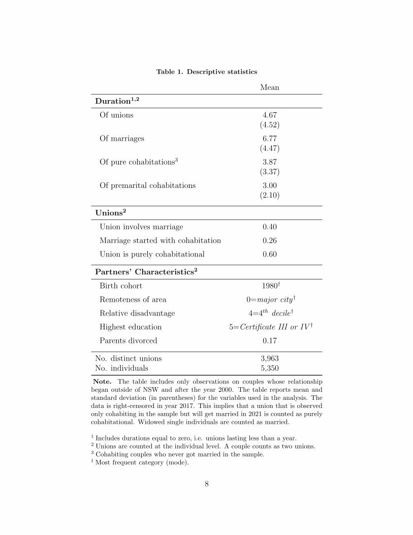
Table 1. Descriptive statistics

Mean

Duration1,2

Of unions 4.67(4.52)

Of marriages 6.77(4.47)

Of pure cohabitations3 3.87(3.37)

Of premarital cohabitations 3.00(2.10)

Unions2

Union involves marriage 0.40

Marriage started with cohabitation 0.26

Union is purely cohabitational 0.60

Partners’ Characteristics2

Birth cohort 1980†

Remoteness of area 0=major city†

Relative disadvantage 4=4th decile†

Highest education 5=Certificate III or IV †

Parents divorced 0.17

No. distinct unions 3,963No. individuals 5,350

Note. The table includes only observations on couples whose relationshipbegan outside of NSW and after the year 2000. The table reports mean andstandard deviation (in parentheses) for the variables used in the analysis. Thedata is right-censored in year 2017. This implies that a union that is observedonly cohabiting in the sample but will get married in 2021 is counted as purelycohabitational. Widowed single individuals are counted as married.

1 Includes durations equal to zero, i.e. unions lasting less than a year.2 Unions are counted at the individual level. A couple counts as two unions.3 Cohabiting couples who never got married in the sample.† Most frequent category (mode).

8

4 Selection Channel

4.1 Identification

The source of identification is the Family Law Amendment Act 2008, since it is exogenously

passed in a particular moment in time. In an ideal setting, I would identify the selection

effect by comparing unions formed just before the reform with unions formed just after. The

unions in the two groups live under the same legal regime, that being the new one. They are

only different in the legal regime under which their union began: the control group started

under the old regime, the treated group under the new one. In the analysis, I keep all the

unions that began in a 3-year window from either side of the reform’s year 2009, i.e. between

2006–2011. The unions that began between 2006-2008 are assigned to the control group and

the ones that began between 2009-2011 are assigned to the treatment group. The choice of

a 3-year window is made in order to increase the sample size2.

4.2 Sample Construction

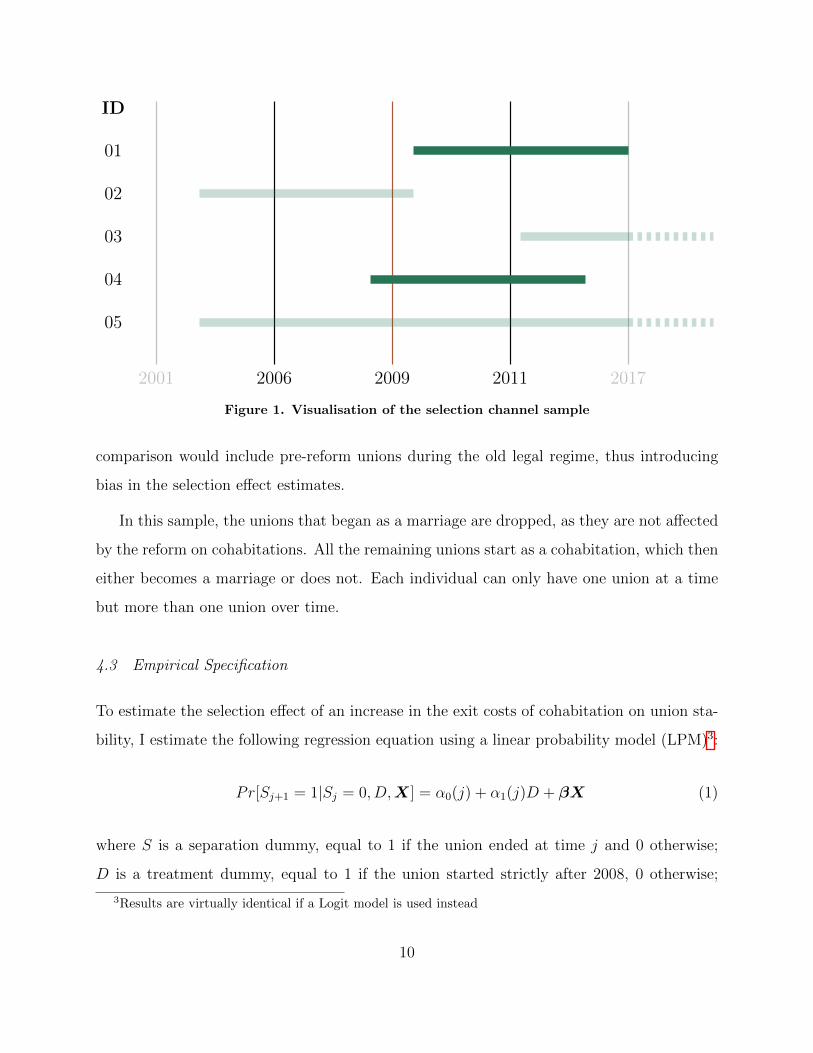
As visualised in Figure 1, the sample for separating the selection channel is constructed by

only keeping unions that started in a 3-year window around the calendar year in which the

reform became active (the darker lines). These unions are then followed over time. Those

unions that started before 2009 are always in the control group, even after 2009, and those

started during or after 2009 are always in the treatment groups, even after 2011.

Furthermore, to better separate selection and incentive effect, the observations on the

first two periods of all unions are dropped. Indeed, unions that began in 2007 remain in the

old legal regime approximately two years before entering the new regime in 2009, during their

third year. Unions started in 2006 remain for two years. In other words, those observations

need to be dropped in order to exclusively compare unions existing under the same regal

regime, which is the object of this section. Conversely, if those initial periods were kept, the

2As shown is Section 4.6 results are robust to the use of a 2-years window

9

2001 2006 2009 2011 2017

ID

01

02

03

04

05

Figure 1. Visualisation of the selection channel sample

comparison would include pre-reform unions during the old legal regime, thus introducing

bias in the selection effect estimates.

In this sample, the unions that began as a marriage are dropped, as they are not affected

by the reform on cohabitations. All the remaining unions start as a cohabitation, which then

either becomes a marriage or does not. Each individual can only have one union at a time

but more than one union over time.

4.3 Empirical Specification

To estimate the selection effect of an increase in the exit costs of cohabitation on union sta-

bility, I estimate the following regression equation using a linear probability model (LPM)3:

Pr[Sj+1 = 1|Sj = 0, D,X] = α0(j) + α1(j)D + βX (1)

where S is a separation dummy, equal to 1 if the union ended at time j and 0 otherwise;

D is a treatment dummy, equal to 1 if the union started strictly after 2008, 0 otherwise;

3Results are virtually identical if a Logit model is used instead

10

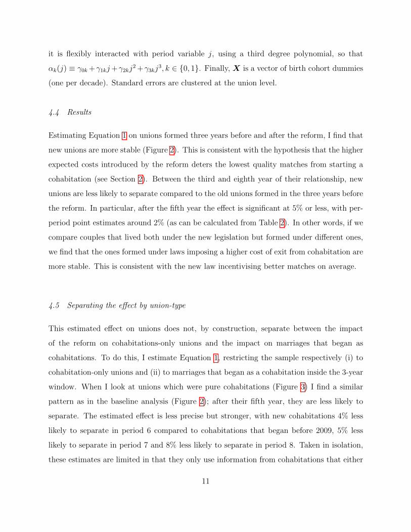
it is flexibly interacted with period variable j, using a third degree polynomial, so that

αk(j) ≡ γ0k +γ1kj+γ2kj2 +γ3kj

3, k ∈ {0, 1}. Finally, X is a vector of birth cohort dummies

(one per decade). Standard errors are clustered at the union level.

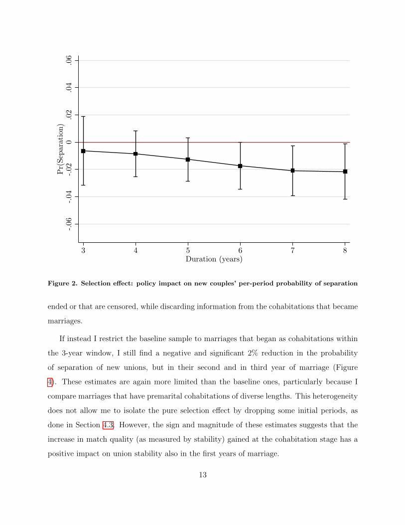
4.4 Results

Estimating Equation 1 on unions formed three years before and after the reform, I find that

new unions are more stable (Figure 2). This is consistent with the hypothesis that the higher

expected costs introduced by the reform deters the lowest quality matches from starting a

cohabitation (see Section 2). Between the third and eighth year of their relationship, new

unions are less likely to separate compared to the old unions formed in the three years before

the reform. In particular, after the fifth year the effect is significant at 5% or less, with per-

period point estimates around 2% (as can be calculated from Table 2). In other words, if we

compare couples that lived both under the new legislation but formed under different ones,

we find that the ones formed under laws imposing a higher cost of exit from cohabitation are

more stable. This is consistent with the new law incentivising better matches on average.

4.5 Separating the effect by union-type

This estimated effect on unions does not, by construction, separate between the impact

of the reform on cohabitations-only unions and the impact on marriages that began as

cohabitations. To do this, I estimate Equation 1, restricting the sample respectively (i) to

cohabitation-only unions and (ii) to marriages that began as a cohabitation inside the 3-year

window. When I look at unions which were pure cohabitations (Figure 3) I find a similar

pattern as in the baseline analysis (Figure 2); after their fifth year, they are less likely to

separate. The estimated effect is less precise but stronger, with new cohabitations 4% less

likely to separate in period 6 compared to cohabitations that began before 2009, 5% less

likely to separate in period 7 and 8% less likely to separate in period 8. Taken in isolation,

these estimates are limited in that they only use information from cohabitations that either

11

Table 2. Selection effect: policyimpact on new unions’ per-periodprobability of separation

(1)Separated

D -0.0290(-0.14)

j -0.129(-1.33)

D × j 0.0180(0.14)

j × j 0.0238(1.29)

D × j × j -0.00432(-0.18)

j × j × j -0.00143(-1.28)

D × j × j × j 0.000273(0.19)

Birth cohort=1940 0.0445∗

(2.41)

Birth cohort=1950 0.0345∗∗∗

(3.73)


(4.88)


(5.88)


(7.34)


(4.50)

Constant 0.225(1.41)

Observations 7202

t statistics in parentheses∗ p < 0.05, ∗∗ p < 0.01, ∗∗∗ p < 0.001

Note. This table presents the LPM es-timates of the impact of the Family LawAmendment Act 2008 on the probabilityof separating for new unions. The inter-action of the treatment D with a thirddegree polynomial of the union’s dura-tion j allows for a compact but flexiblespecification of the policy impact.

12

-.06

-.04

-.02

0.0

2.0

4.0

6P

r(Se

para

tion

)

3 4 5 6 7 8Duration (years)

Figure 2. Selection effect: policy impact on new couples’ per-period probability of separation

ended or that are censored, while discarding information from the cohabitations that became

marriages.

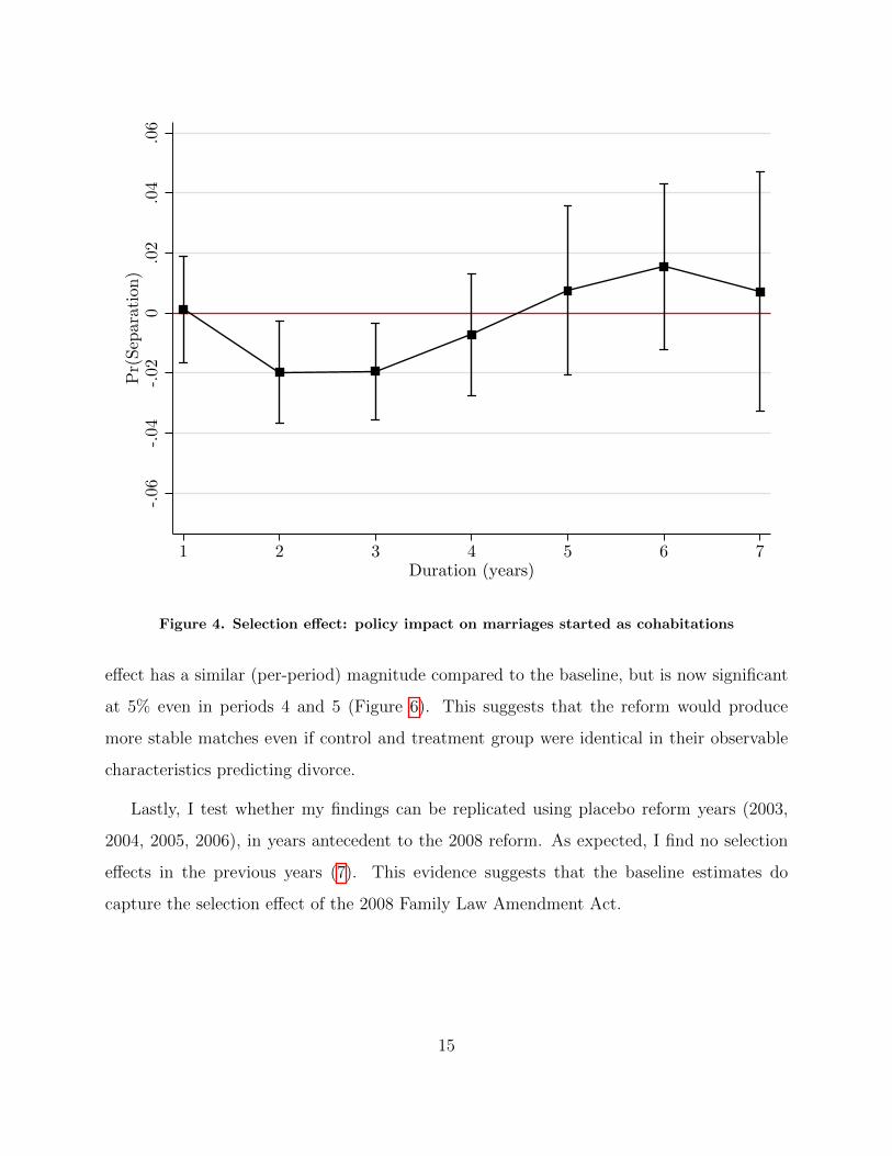
If instead I restrict the baseline sample to marriages that began as cohabitations within

the 3-year window, I still find a negative and significant 2% reduction in the probability

of separation of new unions, but in their second and in third year of marriage (Figure

4). These estimates are again more limited than the baseline ones, particularly because I

compare marriages that have premarital cohabitations of diverse lengths. This heterogeneity

does not allow me to isolate the pure selection effect by dropping some initial periods, as

done in Section 4.3. However, the sign and magnitude of these estimates suggests that the

increase in match quality (as measured by stability) gained at the cohabitation stage has a

positive impact on union stability also in the first years of marriage.

13

-.12

-.1-.0

8-.0

6-.0

4-.0

20

.02

.04

.06

Pr(

Sepa

ration

)


Figure 3. Selection effect: policy impact on purely cohabiting unions

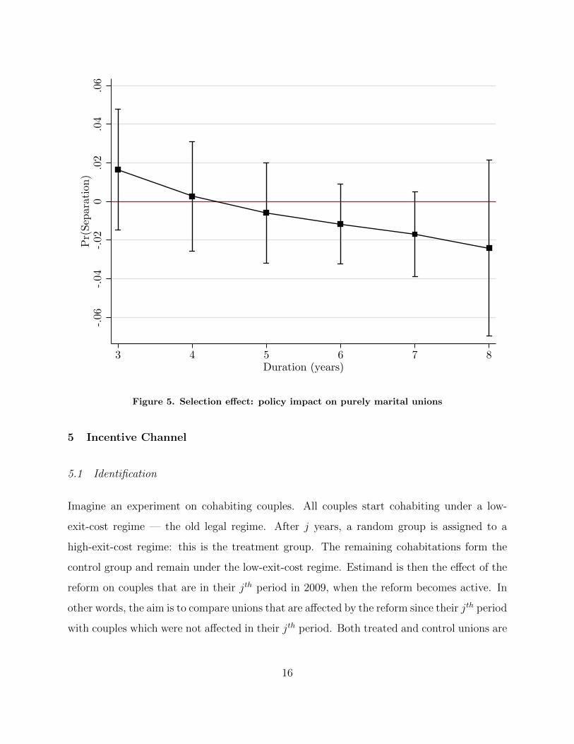
4.6 Robustness Checks

Our policy of interest changes the legislation on cohabiting couples only, hence it should

not affect unions which started as a marriage, without premarital cohabitation. Indeed, I

find that the reform has no statistically significant selection effect on individuals who got

married without cohabiting first (Figure 5). This is further evidence that the baseline results

(Section 4.4) capture the causal effect of the policy of interest, as opposed to capturing some

other general shock to relationship stability.

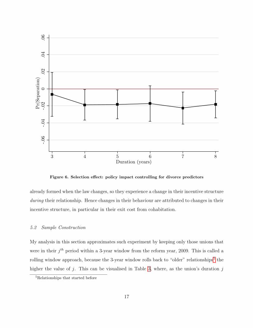
Adding covariates that are correlated with divorce can be useful for balancing the sample4

(see the list in Section 3.2). I add them to Equation 1 and find that the estimated selection

4Here I am using the full selection channel sample, which includes all the types of unions.

14

-.06

-.04

-.02

0.0

2.0

4.0

6P

r(Se

para

tion

)

1 2 3 4 5 6 7Duration (years)

Figure 4. Selection effect: policy impact on marriages started as cohabitations

effect has a similar (per-period) magnitude compared to the baseline, but is now significant

at 5% even in periods 4 and 5 (Figure 6). This suggests that the reform would produce

more stable matches even if control and treatment group were identical in their observable

characteristics predicting divorce.

Lastly, I test whether my findings can be replicated using placebo reform years (2003,

2004, 2005, 2006), in years antecedent to the 2008 reform. As expected, I find no selection

effects in the previous years (7). This evidence suggests that the baseline estimates do

capture the selection effect of the 2008 Family Law Amendment Act.

15

-.06

-.04

-.02

0.0

2.0

4.0

6P

r(Se

para

tion

)


Figure 5. Selection effect: policy impact on purely marital unions

5 Incentive Channel

5.1 Identification

Imagine an experiment on cohabiting couples. All couples start cohabiting under a low-

exit-cost regime — the old legal regime. After j years, a random group is assigned to a

high-exit-cost regime: this is the treatment group. The remaining cohabitations form the

control group and remain under the low-exit-cost regime. Estimand is then the effect of the

reform on couples that are in their jth period in 2009, when the reform becomes active. In

other words, the aim is to compare unions that are affected by the reform since their jth period

with couples which were not affected in their jth period. Both treated and control unions are

16

-.06

-.04

-.02

0.0

2.0

4.0

6P

r(Se

para

tion

)


Figure 6. Selection effect: policy impact controlling for divorce predictors

already formed when the law changes, so they experience a change in their incentive structure

during their relationship. Hence changes in their behaviour are attributed to changes in their

incentive structure, in particular in their exit cost from cohabitation.


My analysis in this section approximates such experiment by keeping only those unions that

were in their jth period within a 3-year window from the reform year, 2009. This is called a

rolling window approach, because the 3-year window rolls back to “older” relationships5 the

higher the value of j. This can be visualised in Table 3, where, as the union’s duration j

5Relationships that started before

17

-.06

-.04

-.02

0.0

2.0

4.0

6P

r(Se

para

tion

)


(a) 2003 placebo reform

-.06

-.04

-.02

0.0

2.0

4.0

6P

r(Se

para

tion

)3 4 5 6 7 8

Duration (years)

(b) 2004 placebo reform

-.06

-.04

-.02

0.0

2.0

4.0

6P

r(Se

para

tion

)


(c) 2005 placebo reform

-.06

-.04

-.02

0.0

2.0

4.0

6P

r(Se

para

tion

)


(d) 2006 placebo reform

Figure 7. Selection channel: placebo effect

18

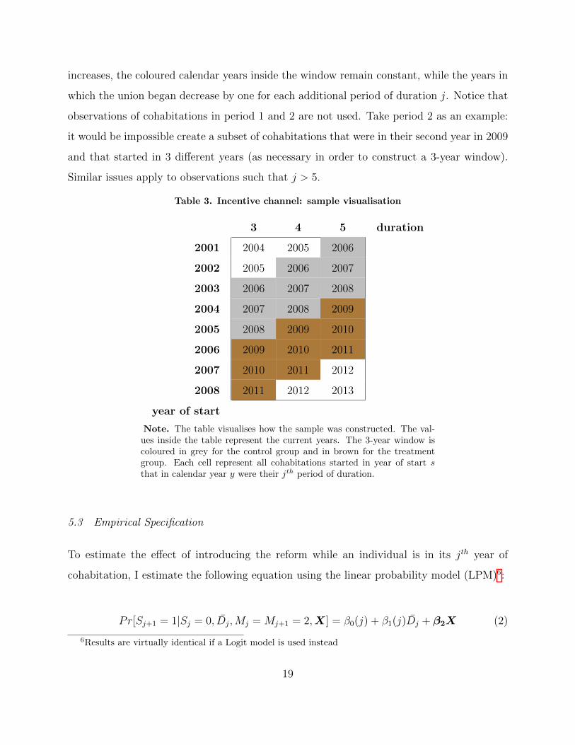
increases, the coloured calendar years inside the window remain constant, while the years in

which the union began decrease by one for each additional period of duration j. Notice that

observations of cohabitations in period 1 and 2 are not used. Take period 2 as an example:

it would be impossible create a subset of cohabitations that were in their second year in 2009

and that started in 3 different years (as necessary in order to construct a 3-year window).

Similar issues apply to observations such that j > 5.

Table 3. Incentive channel: sample visualisation

3 4 5 duration

2001 2004 2005 2006

2002 2005 2006 2007

2003 2006 2007 2008

2004 2007 2008 2009

2005 2008 2009 2010

2006 2009 2010 2011

2007 2010 2011 2012

2008 2011 2012 2013

year of start

Note. The table visualises how the sample was constructed. The val-ues inside the table represent the current years. The 3-year window iscoloured in grey for the control group and in brown for the treatmentgroup. Each cell represent all cohabitations started in year of start sthat in calendar year y were their jth period of duration.


To estimate the effect of introducing the reform while an individual is in its jth year of

cohabitation, I estimate the following equation using the linear probability model (LPM)6:

Pr[Sj+1 = 1|Sj = 0, Dj,Mj = Mj+1 = 2,X] = β0(j) + β1(j)Dj + β2X (2)

6Results are virtually identical if a Logit model is used instead

19

where S is a separation dummy, equal to 1 if the cohabitation ended at time j and 0

otherwise; Dj is a treatment dummy, equal to 1 if the jth period cohabitation takes place

strictly after 2008, 0 otherwise; it is flexibly interacted with period variable j, using a third

degree polynomial, so that βk(j) ≡ γ′0k + γ′1kj + γ′2kj2 + γ′3kj

3, k ∈ {0, 1}; Mj is a marital

status categorical variable equal to 2 if a union is a cohabitation in period j. Finally, X is

a vector of birth cohort dummies (one per decade). Notice also that unions cannot go from

marital to cohabiting. Standard errors are clustered at the union level.

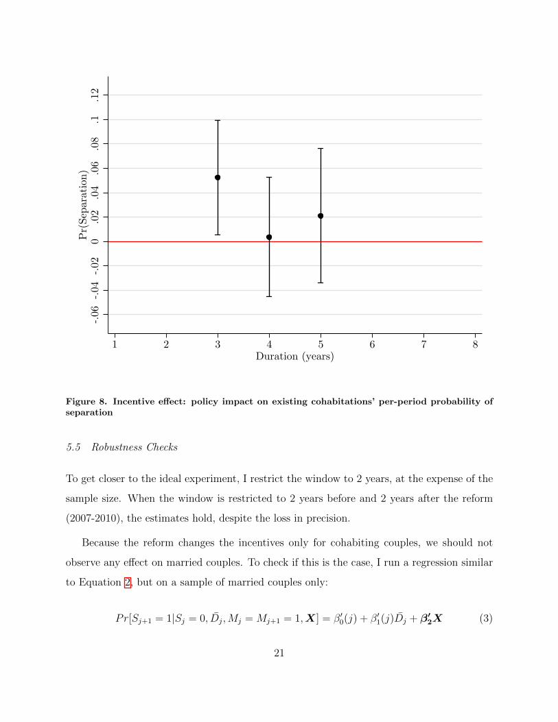
5.4 Results

Individuals who are in their third year of cohabitation in 2009 when the reform becomes

active are 5% more likely to separate. Because the 2009 Family Law Amendment Act does

not define a cohabitation length after which it is classified a de facto relationship, it is

impossible to predict a discontinuity around a specific threshold. However, it is also unlikely

that a cohabitation that has lasted for several years would not be considered as a de facto.

Given this lack of information, individuals might have relied on some rule of thumb, believing

on average that any cohabitation longer than three years would not have been be considered

a de facto relationship. If that were the case, an increase in separation rates in period 3

might come from partners in low quality matches who want to separate before they are

treated as married. However, while New Zealand’s Property (Relationships) Act 1976 sets

the threshold for not being considered a de facto at the end of the third year of cohabitation,

anecdotal evidence from Australia points towards a two-year one (Bryce, 2019). However,

this is not part of the law and it could have emerged more recently. Indeed, if the two-year

rule were followed immediately in 2009, we would have expected higher separation rates in

the second year, close to the threshold for being considered a de facto.

20

-.06

-.04

-.02

0.0

2.0

4.0

6.0

8.1

.12

Pr(

Sepa

ration

)

1 2 3 4 5 6 7 8Duration (years)

Figure 8. Incentive effect: policy impact on existing cohabitations’ per-period probability ofseparation

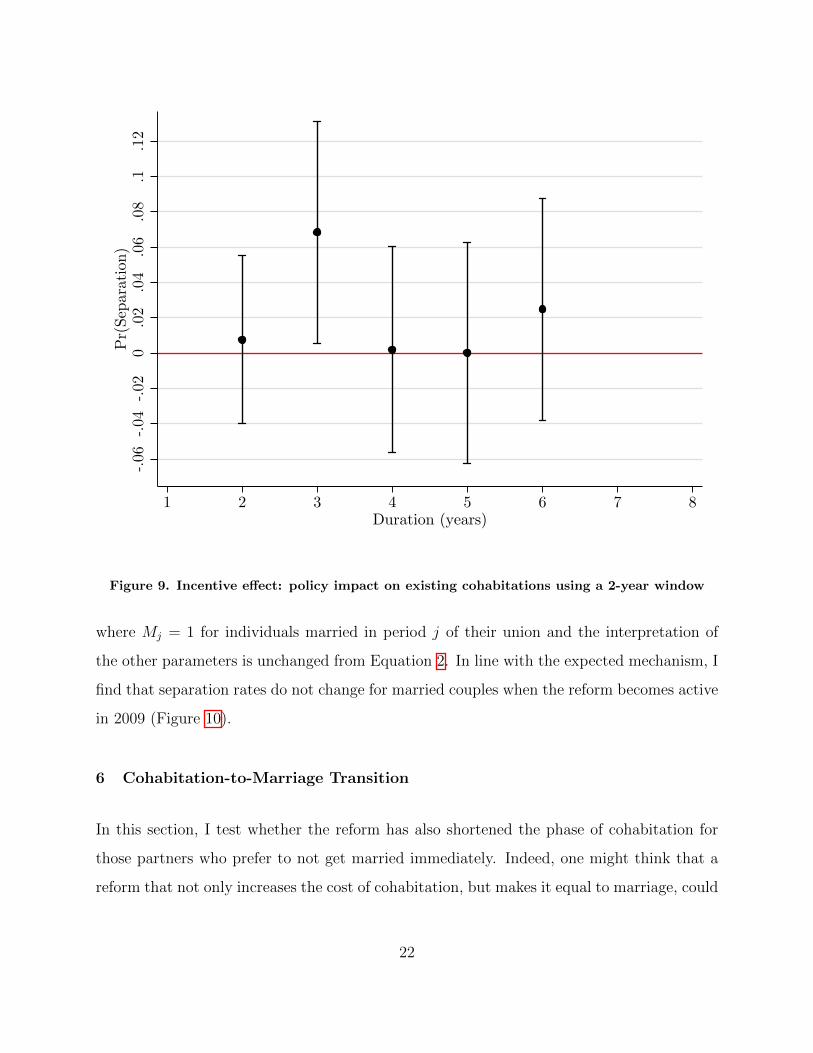
5.5 Robustness Checks

To get closer to the ideal experiment, I restrict the window to 2 years, at the expense of the

sample size. When the window is restricted to 2 years before and 2 years after the reform

(2007-2010), the estimates hold, despite the loss in precision.

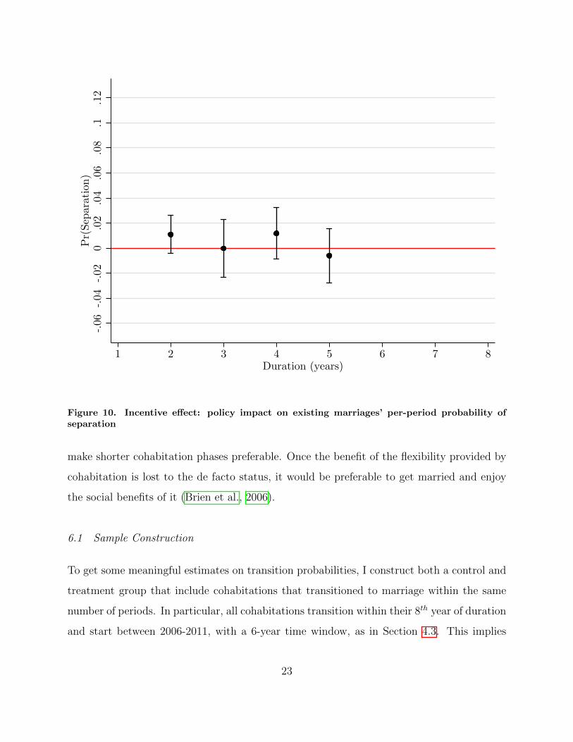
Because the reform changes the incentives only for cohabiting couples, we should not

observe any effect on married couples. To check if this is the case, I run a regression similar

to Equation 2, but on a sample of married couples only:

Pr[Sj+1 = 1|Sj = 0, Dj,Mj = Mj+1 = 1,X] = β′0(j) + β′1(j)Dj + β′2X (3)

21

-.06

-.04

-.02

0.0

2.0

4.0

6.0

8.1

.12

Pr(

Sepa

ration

)


Figure 9. Incentive effect: policy impact on existing cohabitations using a 2-year window

where Mj = 1 for individuals married in period j of their union and the interpretation of

the other parameters is unchanged from Equation 2. In line with the expected mechanism, I

find that separation rates do not change for married couples when the reform becomes active

in 2009 (Figure 10).

6 Cohabitation-to-Marriage Transition

In this section, I test whether the reform has also shortened the phase of cohabitation for

those partners who prefer to not get married immediately. Indeed, one might think that a

reform that not only increases the cost of cohabitation, but makes it equal to marriage, could

22

-.06

-.04

-.02

0.0

2.0

4.0

6.0

8.1

.12

Pr(

Sepa

ration

)


Figure 10. Incentive effect: policy impact on existing marriages’ per-period probability ofseparation

make shorter cohabitation phases preferable. Once the benefit of the flexibility provided by

cohabitation is lost to the de facto status, it would be preferable to get married and enjoy

the social benefits of it (Brien et al., 2006).


To get some meaningful estimates on transition probabilities, I construct both a control and

treatment group that include cohabitations that transitioned to marriage within the same

number of periods. In particular, all cohabitations transition within their 8th year of duration

and start between 2006-2011, with a 6-year time window, as in Section 4.3. This implies

23

that by period 8 all cohabitation will have transitioned to marriage both in the treatment

and in the control groups (by construction). Purely marital unions are dropped from the

sample.


I use a specification identical to Equation 1 to test whether premarital cohabitation has

shortened after the reform:

Pr[Mj+1 = 3|Mj = 2, Sj = 0, Z = 1,X] = α′′0(j) + α′′1(j)D + β′′X (4)

where M = 2 if union is cohabitation and M = 3 if marriage; Z = 1 if a cohabitation

eventually becomes marriage, while it is equal to 0 otherwise. The rest is identically defined

as in Section 4.3.

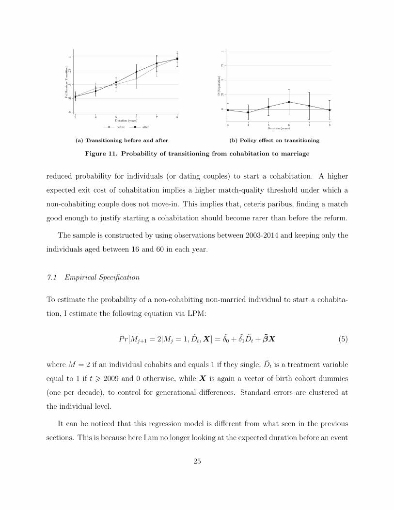
6.3 Results

As Figure 11 shows, premarital cohabitations do not shorten after the reform. This means

that the reform does not cause couples with a preference for a cohabitation phase to change

the timing of their wedding. This result needs further study, as it can be easily shown that

making terminating a cohabitation as expensive as divorce would induce a rational agent to

prefer marriage to cohabitation in any model in which marriage provides an extra benefit

relative to cohabitation. Restricting the window to 1 year, in order to estimate the effects

for initial periods 1 and 2, provides further evidence of no effect (not shown).

7 New Cohabitations & Marriages

Given the claim that the observed increased stability found in Section 4 is due to the crowding

out of low-quality matches7, a decrease in new cohabitations is expected, or, similarly, a

7Which is caused by the higher exit costs of cohabitation

24

0.2

5.5

.75

1P

r(M

arri

age

Tra

nsitio

n)


before after

(a) Transitioning before and after

0.2

5.5

.75

1P

r(Se

para

tion

)


(b) Policy effect on transitioning

Figure 11. Probability of transitioning from cohabitation to marriage

reduced probability for individuals (or dating couples) to start a cohabitation. A higher

expected exit cost of cohabitation implies a higher match-quality threshold under which a

non-cohabiting couple does not move-in. This implies that, ceteris paribus, finding a match

good enough to justify starting a cohabitation should become rarer than before the reform.

The sample is constructed by using observations between 2003-2014 and keeping only the

individuals aged between 16 and 60 in each year.


To estimate the probability of a non-cohabiting non-married individual to start a cohabita-

tion, I estimate the following equation via LPM:

Pr[Mj+1 = 2|Mj = 1, Dt,X] = δ0 + δ1Dt + βX (5)

where M = 2 if an individual cohabits and equals 1 if they single; Dt is a treatment variable

equal to 1 if t > 2009 and 0 otherwise, while X is again a vector of birth cohort dummies

(one per decade), to control for generational differences. Standard errors are clustered at

the individual level.

It can be noticed that this regression model is different from what seen in the previous

sections. This is because here I am no longer looking at the expected duration before an event

25

(separation) occurs. Instead, I am studying whether the yearly probability of an individual

entering a union changes significantly after the reform is passed.

7.2 Results

Following the reform, the probability of starting a cohabitation does not change significantly

(Table 4)8. This finding is inconsistent with most matching models, where higher exit costs

crowd out the lower quality matches (see Matouschek and Rasul, 2008), which leads to a

drop in new matches. To make these models consistent with my findings, one would have

to make additional assumptions, for example higher exit costs making the search for a good

match more efficient. In other words, assuming that high quality matches are scarcer than

low quality matches, if the quality of new cohabitations increases but it remains as likely to

start one, it means that the search for a match has improved on some level.

8 Conclusion

As the way in which people partner changes, governments are called to respond to these

changes. While politicians often introduce regulations aiming at simply ratifying them, we

know that this action is hardly neutral to the outcomes. Indeed, I show that increasing

the expected costs of terminating a cohabitation leads to more stable unions. The positive

effects are not exclusive to cohabitation stability, but spill over into the following marital

phase.

This is inconsistent with standard models of cohabitation and marriage, which assume

that the agent can always rationally rank the different marital states (single, cohabiting,

married) – even during a relationship. Hence standard models do not allow the possibility

that cohabitation might create distortions to rationality by strengthening the romantic at-

tachment of the partners, even in situations in which they do not form a good match. The

psychological literature as put forward such “cohabitation inertia” hypothesis, as detailed in

8This result is robust to the use of a two-way fixed effect model.

26

Table 4. Probability of starting a cohabi-tation

(1)New cohabitation

D -0.00260(-1.73)


(3.53)


(6.68)


(12.50)


(17.91)


(10.48)

Constant 0.0125∗∗∗

(5.16)

Observations 82145

t statistics in parentheses∗ p < 0.05, ∗∗ p < 0.01, ∗∗∗ p < 0.001

Note. This table presents the LPM estimatesof the impact of the Family Law Amendment Act2008 on the probability of starting a new cohab-itation.

Stanley et al. (2006). Stanley et al. (2006) claims that cohabitation makes one more likely to

marry her partner compared to a no-cohabitation scenario. My results are consistent with

cohabitation inertia, providing evidence that policies improving the stability of cohabitation

improve the stability of marriage too. This particularly applies to countries such as Australia

where marriage is mostly preceded by a period of cohabitation.

Other findings are also difficult to reconcile without departing from neoclassical assump-

tions. First, the duration of premarital cohabitation is not affected by the reform. On the

contrary, once marriage and cohabitation are equalled and cohabitation loses its flexibility,

27

premarital cohabitation time for new couples is expected to drop. Secondly, the number of

new cohabitations remains stable after the reform, while all standard models predicts that

it should change with the change in exit costs (Matouschek and Rasul, 2008).

Finally, I find that existing cohabiting unions affected by the reform since their third

year are 10% more likely to separate. This is consistent with the idea that the reform has an

effect on match quality. The lowest quality existing cohabitants do not find worthwhile to

maintain their union under the new exit cost regime, so they break up attempting to escape

it.

From a policy perspective, my findings imply that governments should carefully consider

how they decide to regulate cohabitation. In particular, making cohabitation a choice with

important legal and economic ramifications can help to promote more stable households, to

the benefit of all members.

From a research perspective, this paper shows how cohabitation laws can provide a pre-

cious opportunity to study the causal dynamics at the heart of household formation and

dissolution. Establishing these causal links is the first step on the one hand to identify which

models best explain these dynamics and on the other hand to update such models as to

enable them to reproduce patterns observed in the data.

References

ABS (2011). Socio-economic indexes for areas (seifa). [Cited on page 7.]

Becker, G. S. (1973). A theory of marriage: Part i. Journal of Political Economy, 81(4):813–

846. [Cited on page 1.]

Bishop, W. (1984). ’is he married?’: Marriage as information. The University of Toronto

Law Journal, 34(3):245–262. [Cited on page 1.]

Brien, M. J., Lillard, L. A., and Stern, S. (2006). Cohabitation, marriage, and divorce in

28

a model of match quality*. International Economic Review, 47(2):451–494. [Cited on

page 23.]

Brinig, M. F. and Crafton, S. M. (1994). Marriage and opportunism. The Journal of Legal

Studies, 23(2):869–894. [Cited on page 1.]

Bryce, B. (2019). In a de facto relationship? it won’t save you from the cost of a divorce.

[www.abc.net.au; Updated 6-June-2019]. [Cited on page 20.]

Chiappori, P., Iyigun, M., Lafortune, J., and Weiss, Y. (2017). Changing the Rules Midway:

The Impact of Granting Alimony Rights on Existing and Newly Formed Partnerships.

The Economic Journal, 127(604):1874–1905. [Cited on page 4.]

Chigavazira, A., Fisher, H., Robinson, T., and Zhu, A. (2019). The consequences of extending

equitable property division divorce laws to cohabitants. IZA Discussion Papers, (12102).

[Cited on page 4.]

Cohen, L. (1987). Marriage, divorce, and quasi rents; or, ”i gave him the best years of my

life”. The Journal of Legal Studies, 16(2):267–303. [Cited on page 1.]

Friedberg, L. (1998). Did unilateral divorce raise divorce rates? evidence from panel data.

Working Paper 6398, National Bureau of Economic Research. [Cited on page 2.]

Hewitt, B., Baxter, J., and Western, M. (2005). Marriage breakdown in australia: The

social correlates of separation and divorce. Journal of Sociology, 41(2):163–183. [Cited on

pages 2 and 7.]

Lee, J. Y. and Solon, G. (2011). The fragility of estimated effects of unilateral divorce laws

on divorce rates. Working Paper 16773, National Bureau of Economic Research. [Cited

on page 2.]

Matouschek, N. and Rasul, I. (2008). The economics of the marriage contract: Theories and

evidence. The Journal of Law and Economics, 51(1):59–110. [Cited on pages 1, 2, 4, 26,

and 28.]

29

https://www.abc.net.au/news/2019-06-06/in-a-de-facto-relationship-it-wont-save-you-from-the-cost-/11174252

Mill, J. S. (1994). On the definition and method of political economy. In Hausman, D.,

editor, The philosophy of economics: An anthology, chapter 1, pages 49–51. Cambridge

University Press, Cambridge. [Cited on page 1.]

NSW Government (1984). De facto relationships act 1984 no 147. [Cited on page 5.]

Parliament of Australia (2008). Family law amendment (de facto financial matters and other

measures) act 2008 no 115.

https://www.legislation.gov.au/Details/C2008A00115. [Cited on pages 2, 4, and 5.]

Perelli-Harris, B., Berrington, A., Sanchez Gassen, N., Galezewska, P., and Holland, J. A.

(2017). The rise in divorce and cohabitation: Is there a link? Population and Development

Review, 43(2):303–329. [Cited on pages 1 and 2.]

Stanley, S. M., Rhoades, G. K., and Markman, H. J. (2006). Sliding versus deciding: Iner-

tia and the premarital cohabitation effect*. Family Relations, 55(4):499–509. [Cited on

page 27.]

Wolfers, J. (2006). Did unilateral divorce laws raise divorce rates? a reconciliation and new

results. American Economic Review, 96(5):1802–1820. [Cited on page 2.]

30

https://www.legislation.gov.au/Details/C2008A00115

de facto marriage: when ending a cohabitation costs as

Documents