DC Characterization and 3D Modelling of a Triangular, Epoxy-Impregnated High

Temperature Superconducting (HTS) Coil

D Hu1, M D Ainslie1, J P Rush1, J H Durrell1, J Zou1, M J Raine2, D P Hampshire2

1Bulk Superconductivity Group, Department of Engineering, University of Cambridge, Trumpington

Street, Cambridge, CB2 1PZ, UK

2Superconductivity Group, Centre for Materials Physics, Department of Physics, University of

Durham, South Road, Durham, DH1 3LE, UK

E-mail: dh455@cam.ac.uk

Abstract

The direct current (DC) characterization of high temperature superconducting (HTS) coils is

important for applications, such as electric machines, superconducting magnetic energy storage

(SMES) and transformers. In this paper, the DC characterization of a triangular-shaped, epoxy-

impregnated HTS coil wound with YBCO coated conductor intended for use in an axial-flux HTS

motor is presented. Voltage was measured at several points along the coil to provide detailed

information of its DC characteristics. The coil is modelled based on the H-formulation using a new 3D

technique that utilizes the real superconducting layer thickness, and this model allows simulation of

the actual geometrical layout of the HTS coil structure. Detailed information on the critical current

density’s dependence on the magnitude and orientation of the magnetic flux density, Jc(B,θ),

determined from experimental measurement of a short sample of the coated conductor comprising

the coil is included directly in the numerical model by a two-variable direct interpolation to avoid

developing complicated equations for data fitting and greatly improve the computational speed.

Issues related to meshing the finite elements of the real thickness 3D model are also discussed in

detail. Based on a comparison of the measurement and simulation results, it is found that non-

uniformity along the length exists in the coil, which implies imperfect superconducting properties in

the coated conductor, and hence, coil. By evaluating the current-voltage (I-V) curves using the

experimental data, and after taking into account a more practical n value and critical current for the

non-uniform region, the modelling results show good agreement with the experimental results,

validating this model as an appropriate tool to estimate the DC I-V relationship of a superconducting

coil. This work provides a further step towards effective and efficient 3D modelling of

superconducting devices for large-scale applications.

1. Introduction

In recent years, long-length, high-quality high temperature superconducting (HTS) tapes have

become commercially available, which increases the potential of practical, large-scale HTS

applications. The direct current (DC) characterization of high temperature superconducting (HTS)

coils is important for HTS applications, such as electric machines, superconducting magnetic energy

storage (SMES) and transformers. The DC properties can help determine the maximum allowable

current in an HTS electric machine, which has a large impact on the size and weight of the machine,

and hence, its power density [1-3]. We are investigating the design of an all-superconducting axial

flux-type electric machine [4] and currently carrying out the DC characterization of HTS coils wound

from YBCO coated conductors for the stator winding of the machine. A triangular-shaped HTS coil is

one of the test candidates of this superconducting stator, which is commonly used, along with

trapezoidal and circular designs, in conventional axial flux-type machines.

The analysis of the electromagnetic behaviour of superconducting materials based on the finite

element method (FEM) can predict their performance for practical devices, such as HTS electrical

machines [5-10], and assist in interpreting experiment results. There are three main formulations for

FEM calculations: the H-formulation [11-14], the A-V formulation [15-18] and the T-Ω formulation

[19-21]. Maxwell’s equations can be written in each of these formulations and these formulations

are equivalent in principle, but the solutions of the corresponding partial differential equations

(PDEs) can be very different [22]. A more general overview of the potential and limits of numerical

modelling for supporting the development of HTS devices is presented in [23].

A number of groups have reported research on the application of the H-formulation [3,5,6,8-14,24-

34] and several authors have investigated the electromagnetic properties of HTS coils based on this

method [3,5,6,9,10,24,30,31,34-36]. However, to our knowledge, there exists no three-dimensional

(3D) HTS coil model using the H-formulation that utilises the real superconducting layer thickness. A

3D model with the real superconducting layer thickness can analyse the electromagnetic behaviour

of superconducting coils under complex geometries (i.e., those without a two-dimensional (2D)

symmetric equivalent) and situations accurately. In addition, this technology can simulate HTS

coated conductors with a magnetic substrate or other layers easily, which is applied in a similar way

to the 2D method [26,31].

In this paper, the DC characterization of a triangular-shaped HTS coil made from YBCO coated

conductor for a prototype axial flux HTS electric machine is presented. Multiple voltage taps were

used during measurement to provide detailed information on the DC characterization of the coil. A

3D coil model with the real superconducting layer thickness based on the H-formulation,

implemented using the commercial FEM software package COMSOL Multiphysics 4.3a [37], is

proposed to simulate the electromagnetic properties of the triangular coil.

In Section 2, the experimental details are described, including detailed information on the critical

current density’s dependence on the magnitude and orientation of the magnetic flux density, Jc(B,θ),

determined from measurement of a short sample from the coated conductor comprising the coils.

The Jc(B,θ) data is directly included in the numerical model by a two-variable direct interpolation to

avoid developing complicated equations for data fitting. In Section 3, the 3D FEM model framework

is described and issues related to meshing the real thickness 3D model is discussed in details. In

Section 4, the experiment and simulation results are compared and it is found that

inhomogeneities/non-uniformities along the length [38-40] exist in the tested coil. Based on the

experimental data and modelling results, the inhomogeneous superconducting properties of the

coated conductor are analysed in detail, highlighting the usefulness of such numerical techniques in

interpreting experimental results.

2. DC Characterization and Tape Properties

The triangular, HTS pancake coil used in this study was wound using SuperPower SCS4050-AP coated

conductor [41] and then impregnated in epoxy. A photograph of the coil is shown in Figure 1. The

total length of tape used was 18.6 m, resulting in 37 layers of silk ribbon interleave, vacuum

impregnated with epoxy resin. The vacuum impregnation process included a 10 bar overpressure

with nitrogen gas, which was maintained for 4-5 hours before rotary baking. The resin used was

stycast W19 with catalyst 11 in the ratio of 100:17. The specifications of the HTS coated conductor

used [41] and the test coil are listed in Table 1.

Figure 1. The triangular, HTS pancake coil used in this study.

Table 1. Specification of the coated conductor and triangular, HTS pancake coil

PARAMETER TRIANGULAR PANCAKE COIL

Tape manufacturer SuperPower

Tape type SCS4050-AP

Critical current [self-field, 77 K] 94.7 A

Conductor width, w 4 mm

Conductor thickness, dc 0.1 mm

YBCO layer thickness, dsc 1 µm

Distance between YBCO layers Approximately 220 µm

Length of conductor used 18.6 m

Coil turns, nc 37

Coil side length 147 mm

Bend radius of coil corners 20 mm

For the triangular coil shown in Figure 1, the length of each side, measured from the centre of the

corner bend at the outer turn, is 147 mm, and the distance between the top and bottom sides,

measured from the inner turn, is 137 mm. The radius of the inner turn at each corner bend is 20 mm,

which is larger than the minimum bend radius of the conductor (11 mm).

Ten voltage taps were utilised within the coil to help provide further detailed information for the DC

characterization of the coil. By pairing the voltage taps, there are 13 voltage sections used for the

measurements, as shown in Figure 2. The voltages V1-V9 are the voltages between the individual taps,

which are spaced approximately every 2 m along the tape length, except for the final voltage tap,

which is located 1.4 m from its preceding tap. The first voltage tap is wired 1 m from the coil’s inner

copper current contact and the final voltage tap is wired 0.2 m from the outer current contact to

prevent an anomalous measurement due to localised heating of the tape near the coil terminals [34].

Hence, V1 corresponds to the voltage across the innermost section of the coil and V9 corresponds to

the outermost section. V10, V11, and V12 correspond to the voltages along each third of the coil,

where V10 = V1 + V2 + V3, V11 = V4 + V5 + V6, and V12 = V7 + V8 + V9, and V13 is total coil voltage across a

17.4 m tape length.

Figure 2. The specific voltage taps and measured voltages for the triangular, HTS pancake coil.

The coil was cooled slowly to 77 K over several hours using liquid nitrogen vapour, followed by

submersion in a liquid nitrogen bath. The current-voltage (I-V) curves of the coil and across the

different voltage sections were recorded. The coil current was supplied by a DC power supply with a

ramp-rate 0.5 A/s to reduce the influence of the inductance of the coil. For the experimental

measurement, as well as the numerical modelling, the critical current of the coil/voltage section is

defined as the DC current when the electric field across a region reaches the characteristic electric

field E0 = 1 µV/cm [42,43] – this may be converted to a characteristic voltage using the distance

between two taps. The DC measurements were repeated to confirm the reproducibility of the

measurements and check for any thermal cycling effects, of which there was none.

Before winding the coil, the angular dependence Jc(B,θ) of the critical current, which is defined in

Figure 3, of a short sample from the spool of tape used to wind the coil was measured, the results of

which are shown in Figure 4. The magnitude of the applied field was varied from 0 to 0.7 T in 0.1 T

increments.

Figure 3. The definition of angular dependence Jc(B,θ) of the critical current.

Figure 4. Measured angular dependence Jc(B,θ) of the critical current of a short sample from the

spool of tape used to wind the test coil.

In [44], the authors introduced an elliptical fitting function to represent the Jc(B,θ) relationship. In

[40,45], the authors developed a method to describe a more complex Jc(B,θ) relationship for coated

conductors using 11 parameters with good agreement with experimental results. In [30], an

alternative method was developed, based on measurements of the reduction in critical current due

to parallel and perpendicular fields, using an angular function G(θ) for a particular applied field (100

mT in that paper). This also achieved good fitting of experiment data.

Here we propose a simpler method; a two-variable direct interpolation method, which completely

avoids any complex data fitting process for Jc(B,θ) and expresses the anisotropic behaviour in the

FEM software directly and accurately. The measured Jc(B,θ) data shown in Figure 4 can be input

directly as a single function, with two input variables, B and θ, and one output variable, Jc,

automatically using a direct interpolation in COMSOL. This significantly simplifies the whole process

whilst maintaining the highest possible accuracy for the input data. Symmetric behaviour is assumed

for angles 90° < θ < 270°.

3. 3D Numerical Analysis Framework

A finite element-based model based on 3D H-formulation is used to investigate the electromagnetic

properties of the HTS coil. Considering the actual geometry of the test coil, the triangular coil needs

to be modelled in 3D. 3D models of HTS materials have been developed by several groups using

different formulations to carry out the numerical FEM calculations [18,21,27,32,46-48]. The H-

formulation is considered in this paper because models based on H-formulation can converge

quickly and it is easy to impose electromagnetic boundary conditions related to the current flowing

in the conductors [6] or to apply an external magnetic field, if required [49]. The introduction of the

Jc(B,θ) relationship is straightforward, too, since the magnetic field variable is available directly [23].

Furthermore, although 3D models of HTS materials based on H-formulation have been developed -

for a single tape [27], bulk superconductors [27-29], two coupled tapes and helically-wound wires

[32], Roebel cables [33], and coils using a direct [36] or homogenized [35] bulk approximation –

there exists no 3D HTS coil model using both the H-formulation and the real superconducting layer

thickness, which is developed here.

3.1 Governing Equations

Similar to previous studies [27-29,32,33,35,36], the governing equations for the 3D H-formulation

are derived from two of Maxwell’s equations: Faraday’s law (1) and Ampere’s law (2).

0d( )d

0dt dt

rμ μ

HBE E (1)

H J (2)

where H = [Hx, Hy, Hz] represents the magnetic field components, J = [Jx, Jy, Jz] represents the current

density and E = [Ex, Ey, Ez] represents the electric field components. µ0 is the permeability of free

space. For the superconducting layers and air subdomains, the relative permeability µr = 1.

It is assumed that the electric field E is parallel to the current density J [3,27-36] and the electrical

properties of the superconductor are modelled by the E-J power law [50,51] given in (3).

0( )

( , )c

n

J BE

JE (3)

where E0 is the characteristic electric field 1 µV/cm as described in Section 2. For HTS materials, n is

usually within the range of 5 (strong flux creep) and 50 (limiting value for HTS and LTS materials)

[6,17,50]. When n > 20, it becomes a good approximation of Bean’s critical state model [46].

Therefore, in this paper, we assume n = 21.

The knowledge of the in-field critical current density behaviour, Jc (B,θ), of the coated conductor

used to wind the coil is input as a two-variable direct interpolation of the experimental data (Figure

4) into COMSOL, where B is the magnitude of the local magnetic flux density and θ is the angle with

respect to the top surface of the tape (Figure 3). In order to derive these two parameters, B⊥ and B‖, ,

which represent the perpendicular and parallel components of the flux density, respectively, can be

expressed depending on the specific geometrical structure, where 2 2B B B

and θ =

arctan(B⊥/B‖). For non-superconducting subdomains (e.g., the air between the tapes and

surrounding the coil), a linear Ohm’s law is considered, E = ρJ, where ρ is the specific, constant

resistivity for the material.

3.2 Geometry, Boundary Conditions & Current Constraints

Considering the high mesh density and computation time required for a full 3D model, geometry

symmetry is made use of, as shown in Figure 5: only 1/6th of the length of the coil is modelled using

symmetric boundary conditions.

Figure 5. 1/6th of the length of the coil is modelled using symmetric boundary conditions.

In this paper, since only the transport current problem is addressed and no external magnetic field is

applied, Dirichlet boundary conditions [6,29,33] are applied such that Hx = Hy = Hz = 0, for a

sufficiently large air subdomain. Neumann boundary conditions are applied to describe the magnetic

field continuity between the air and superconductor subdomains. Finally, integral constraints are

applied to the superconducting layers to represent the particular transport current flowing in the

coil. A transport current Is through any surface s can be described as follows:

ts J dsI S (4)

where St represents the local unit vector tangential to the cross-section of the superconducting layer.

3.3 Mesh Considerations

The mesh is a key factor for finite element analysis and the selection of an appropriate mesh method

is crucial for accurate and fast simulations. For the real thickness 3D coil model, it is found that the

combinations of different mesh methods can decrease the number of mesh element and degrees of

freedom effectively, whilst maintaining good accuracy and convergence during the simulation.

Mesh scaling and mapped meshing are both good methods to improve the convergence speed and

reduce the simulation time required. A mapped mesh [6] is applied in the 2D cross-section of the

HTS coated conductor, as shown in Figure 6, to decrease the number of mesh elements. For clarity,

there are only four layers of the coil shown and only half of each conductor because of geometrical

symmetry. Mesh scaling is another effective method to reduce the number of created elements,

which scales the geometry along the thin direction before meshing and then scales the mesh back to

fit the mesh in the original geometry. This is applied to the cross-section of the air subdomain

between the superconducting tapes. A mapped mesh can be also applied to the air subdomain

between the superconducting tapes [6]; however, the reason that mesh scaling is recommended in

the region of air domain between the HTS tapes is that mesh scaling in that region of the coil model

improves convergence and speed at least one order of magnitude over a mapped mesh, without

reduction in accuracy. Therefore, such a combined mapped-scaled mesh is a good method for

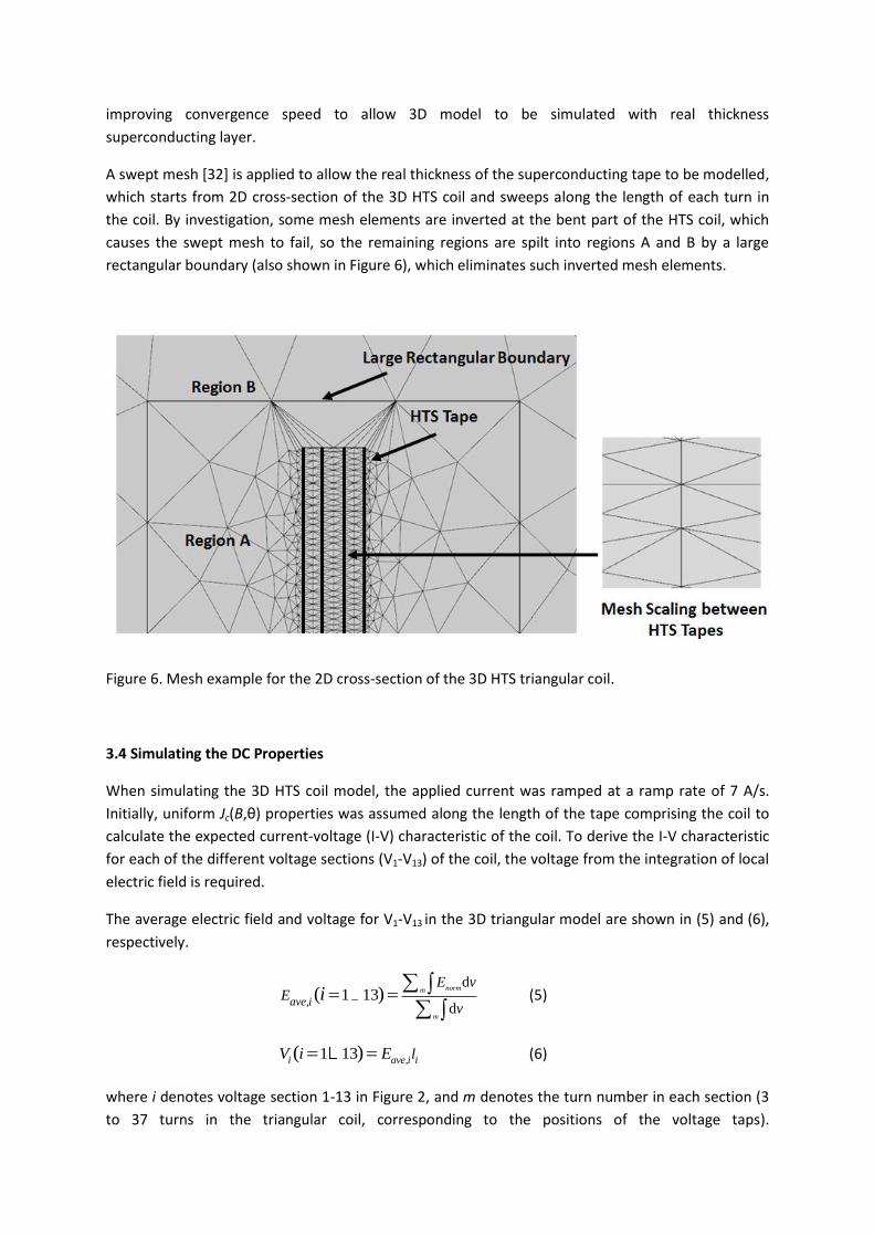
improving convergence speed to allow 3D model to be simulated with real thickness

superconducting layer.

A swept mesh [32] is applied to allow the real thickness of the superconducting tape to be modelled,

which starts from 2D cross-section of the 3D HTS coil and sweeps along the length of each turn in

the coil. By investigation, some mesh elements are inverted at the bent part of the HTS coil, which

causes the swept mesh to fail, so the remaining regions are spilt into regions A and B by a large

rectangular boundary (also shown in Figure 6), which eliminates such inverted mesh elements.

Figure 6. Mesh example for the 2D cross-section of the 3D HTS triangular coil.

3.4 Simulating the DC Properties

When simulating the 3D HTS coil model, the applied current was ramped at a ramp rate of 7 A/s.

Initially, uniform Jc(B,θ) properties was assumed along the length of the tape comprising the coil to

calculate the expected current-voltage (I-V) characteristic of the coil. To derive the I-V characteristic

for each of the different voltage sections (V1-V13) of the coil, the voltage from the integration of local

electric field is required.

The average electric field and voltage for V1-V13 in the 3D triangular model are shown in (5) and (6),

respectively.

,

d

d1 13( )

normm

m

ave i

E vE

vi

(5)

,1 13( )i ave i ilV i E (6)

where i denotes voltage section 1-13 in Figure 2, and m denotes the turn number in each section (3

to 37 turns in the triangular coil, corresponding to the positions of the voltage taps).

2 2 2norm x y zEE E E represents the local electric field in the triangular coil. v represents the

volume of each turn m and the term dm

v is the volume sum of these m turns. li represents the

wire length of each voltage section. Taking voltage section 1 as an example, m varies from 3 to 6.

Based on (5) and (6), the average electric field Eave,1 and voltage V1 for voltage section 1 of the

triangular coil can be calculated.

4. Results & Discussion

The predicted I-V curve from the numerical analysis and the DC measurement results for the

triangular coil are shown in Figure 7. V13 is the total coil voltage, as shown in Figure 2.

Figure 7. Comparison of current-voltage (I-V) curves for the simulation and experimental results for

the triangular coil. The simulation initially assumed uniform Jc(B,θ) properties along the length of the

tape comprising the coil.

Based on Figure 7, the experimental result indicates a critical current for the coil of around 38 A, and

the simulation result, based on the previous assumptions, estimates a critical current of around 63 A,

indicating a large discrepancy between the two. The simulated curve is based on the measured Jc (B,

θ) behaviour of a short sample and assumes uniform properties along length of conductor in the coil.

Here, we investigate the uniformity of the coil in more detail using the experimentally measured

results.

The measured I-V curves for V10–V13 are shown in Figure 8, where V10, V11 and V12 are the I-V curves

for each third of the coil. In addition, the measured, average electric field for voltage sections V1–V9

when the input current reaches the critical current of the triangular coil, and the test data for the

critical current every 5 m along the conductor (provided by the manufacturer) are shown in Figure 9.

Figure 8. Current-voltage (I-V) curves for each third of the coil, corresponding to V10, V11 and V12, and

the total coil voltage, V13.

Figure 9 (a) The average electric field for voltage sections V1–V9 (b) The test data for the critical

current every 5 m along the conductor, provided by the manufacturer.

Based on Figures 8, 9(a) and 9(b), non-uniformity of the critical current exists along the length of the

HTS triangular coil. Based on Figure 9(a), the maximum electric field, corresponding to the region of

lowest critical current in the coil, exists between 5 m and 7 m (voltage V3 in the triangular coil).

Based on Figure 9(b), there are regions of comparatively lower critical current between 4 m and 14

m, indicating overlap between the maximum electric field and lower critical current.

The previous assumption of uniform critical current density along the length of tape is unreasonable

due to the presence of this non-uniformity along its length. If one were to assume uniform

properties, it is expected that the inner turn at the bends/corners will see a relatively higher

localised magnetic field, which would determine the overall critical current of the coil [31,49].

It is a common phenomenon that some non-uniformity exists along the length of an HTS coated

conductor [2,38-40,52-61]. Non-uniformity along the length [38-40,54] can be a crucial concern in

HTS coils and the performance of the coated conductor can be influenced by many factors, such as

the processing of the material [38,39,52-55,58] or winding of the coil [2,56,57,59-61]. In terms of

material processing [38,39,52-55,58], the percentage of doping in the HTS tape, the deposition rate,

and the roughness of the surface of the tape can have a significant impact on the uniformity over

long lengths. From data along long lengths from manufacturers and research institutions [38,39,52-

55,58], it can be seen that the critical current in self-field along the length can vary, sometimes

suddenly in particular, localised sections. If the angular dependence of critical current density for a

specific magnetic field is also considered, the difference may become more obvious and one such

case can be seen in [38].

In terms of winding the coil [2,56,57,59-61], the HTS tape is sensitive to bending strain, which can

lead to a decrease in the critical current of the coil. The specific reason for the non-uniformity along

the length in this particular case is beyond the scope of our investigations, but utmost care was

taken during the winding process to avoid excessive strain.

Based on Figure 9(a), there is a significant electric field generated only in voltage section V3 of the

coil, which also dominates the voltage of the whole coil. For the other regions of the triangular coil,

there are comparatively lower electric fields. Following [59], an approximation of uniform Jc(B,θ) can

be made within each section, whether non-uniform (section V3) or uniform (all other voltage

sections). Using the experimental results for the non-uniform region, as shown in Figure 10, a more

realistic Jc(B,θ) and n value can be calculated for this particular region.

Figure 10. Current-voltage (I-V) characteristic for voltage section V3 of the triangular coil used to re-

calculate a more realistic Jc(B,θ) and n value for this particular non-uniform region.

Following [59], the critical current of this region is 14 A and the n value cannot be considered

constant. When the current is over 14 A, n = 1.98 and below 14 A, n = 3.63.

In order to estimate the critical current of the tape in V3 based on information in Figure 4, the

average magnetic field magnitude and orientation in this region are needed. To derive the average

magnetic field magnitude and its orientation in voltage sections, the integration of local magnetic

field magnitude and orientation is needed. The average magnetic field magnitude and its orientation

for V1-V13 in the 3D model are shown in equations (7) and (8), respectively.

,

d

d1 13( ) m

m

ave i

B vB

vi

(7)

,

d

d1 13( ) m

m

ave i

v

vi

(8)

where i denotes voltage section 1-13 in Figure 2, and m denotes turn number in each section (3 to

37 turns in the triangular coil, corresponding to the positions of the voltage taps). B and θ represent

the local flux density magnitude and its orientation, respectively. As per equation (5), v represents

the volume of turn m.

Based on the previous ideal coil model (with the approximation of uniform critical current along the

entire length of the tape in the whole winding) and equations (7), (8), the average magnetic field B =

0.014 T and angle θ = 6° in V3 when the applied current is 14 A. Considering the Jc(B,θ) data

presented in Figure 4, the critical current of the tape in that region is Ic(0.014 T,6°) = 93 A. Here, the

same Jc(B,θ) behaviour is assumed, but the magnitude of Jc(B,θ) is assumed to decrease in

proportion. Therefore, the new critical current density in the non-uniform region is fixed to

Jc(B,θ)x14/93 with the previous critical current density for all other (uniform) regions, as shown in

Table 2. Using this information, the new simulated I-V curves are compared with the experimental

measurements using the average electric field [34,40] and the results are shown in Figure 11.

Table 2. n value and critical current density of the triangular pancake coils

REGIONS n VALUE CRITICAL CURRENT DENSITY

Non-uniform V3 Region 3.63 (I < 14 A)

1.98 (I > 14 A)

14( , )

93cJ B θ

Other uniform regions

(V1, V2, V4–V9)

21 Jc(B,θ)

Figure 11. A comparison of calculated and experiment results, using the average electric field, for the

current-voltage (I-V) curves when simulating a region of non-uniformity in the coil.

From Figure 11, it can be seen that experiment results are now almost consistent with the simulation

results, when taking into account the non-uniform V3 region in the coil, resulting in a large voltage

generated in this region, which impacts significantly on the overall coil voltage and hence critical

current. V3 represents the non-uniform region and V13-V3 represents the uniform regions. From

Figure 11, it can be seen that 3D HTS model can simulate both uniform and non-uniform regions and

the results match well with the experimental results. The consistence of the modelling and

experimental results demonstrates this 3D model as an effective tool to estimate current-voltage

relationship of a superconducting coil, especially for those without a two-dimensional (2D)

symmetric equivalent, such as racetrack and triangular coils.

At the same time, the 3D finite element model can also express field distribution and current density

distribution accurately and it makes a valuable tool for coil optimization. It can be even extended as

part of superconducting machine, which cannot be simply simulated by 2D models, and provides a

further step towards effective and efficient 3D modelling of large-scale HTS applications.

5. Conclusion

In this paper, the DC properties of a triangular, epoxy-impregnated HTS coil made from YBCO coated

conductor for a prototype axial flux HTS electric machine were measured. Multiple voltage taps were

utilized within the coil during measurement to help provide further detailed information on the DC

characterization of the coil.

A 3D numerical model, based on the H-formulation and including the real superconducting layer

thickness, is implemented using the commercial FEM software package COMSOL Multiphysics 4.3a

to simulate the electromagnetic properties of the coil. Detailed information on the critical current

density’s dependence on the magnitude and orientation of the magnetic flux density, Jc(B,θ),

determined from experimental measurement of a short sample of the coated conductor comprising

the coil is included directly in the numerical model by a two-variable direct interpolation to avoid

developing complicated equations for data fitting and greatly improve the computational speed. In

addition, a combined mapped-scaled mesh is proposed for improving the model’s convergence to

allow a fast and efficient 3D simulation including the real thickness of the superconducting layer.

Numerical analysis can help us understand the experiment result, and based on the comparison of

measurement and simulation results, it is found that non-uniformity along the length exists in the

coil. By evaluating the current-voltage (I-V) curves using experimental data, a decreased n value and

critical current is observed in a non-uniform region of the coil. When the 3D model is modified to

account for this practical critical current and n value, the experiment and modelling results show

good agreement, validating this 3D model as an effective tool to estimate DC I-V relationship of a

superconducting coil. At the same time, this model allows the development of an effective and

efficient 3D model for analysing large-scale HTS applications.

Acknowledgements

Di Hu and Jin Zou would like to acknowledge the support of Churchill College, Cambridge, the China

Scholarship Council and the Cambridge Commonwealth, European and International Trust. Dr Mark

Ainslie would like to acknowledge the support of a Royal Academy of Engineering Research

Fellowship.

References

[1] Konishi T, Nakamura T, Nishimura T and Amemiya N 2011 IEEE Trans. Appl. Supercond. 21 1123-6

[2] Oomen M, Herkert W, Bayer D, Kummeth P, Nick W and Arndt T 2012 Physica C 482 111-8

[3] Hu D, Ainslie M D, Zou J and Cardwell D A 2015 IEEE Trans. Appl. Supercond. 25 4900605

[4] Ainslie M D, George A, Shaw R, Dawson L, Winfield A, Steketee M and Stockley S 2014 J. Phys.: Conf. Ser. 507 032002

[5] Ainslie M D, Jiang Y, Xian W, Hong Z, Yuan W, Pei R, Flack T J and Coombs T A 2010 Physica C 470 1752-5

[6] Ainslie M D, Rodriguez-Zermeno V M, Hong Z, Yuan W, Flack T J and Coombs T A 2011 Supercond.Sci. Technol. 24 045005

[7] Jin J X, Zheng L H, Guo Y G, Zhu J G, Grantham C, Sorrell C C and Xu W 2012 IEEE Trans. Appl. Supercond. 22 5202617

[8] Queval L and Ohsaki H 2013 IEEE Trans. Appl. Supercond.23 5201905

[9] Messina G, Morici L, Vetrella U B, Celentano, Marchetti M, Viola R and Sabatino P 2014 J. Phys.: Conf. Ser. 507 032031

[10] Messina G, Morici L, Vetrella U B, Celentano G, Marchetti M, Sabatino P and Viola R 2014 IEEE Trans. Appl. Supercond. 24 4602204

[11] Pecher R, McCulloch M D, Chapman S J, Prigozhin L and Elliott C M 2003 Proc. 6th EUCAS pp 1-11

[12] Kajikawa K, Hayashi T, Yoshida R, Iwakuma M and Funaki K 2003 IEEE Trans. Appl. Supercond. 13 3630

[13] Hong Z, Campbell A M and Coombs T A 2006 Supercond. Sci. Technol. 19 1246-52

[14] Brambilla R, Grilli F and Martini L 2007 Supercond. Sci. Technol. 20 16-24

[15] Prigozhin L 1997 IEEE Trans. Appl. Supercond. 7 3866-73

[16] Barnes G, McCulloch M and Dew-Hughes D 1999 Supercond. Sci. Technol. 12 518-22

[17] Stavrev S, Grilli F, Dutoit B, Nibbio N, Vinot E, Klutsch I, Meunier G, Tixador P, Yang Y and Martinez E 2002 IEEE Trans. Magn. 38 849-52

[18] Campbell A M 2009 Supercond. Sci. Technol. 22 034005

[19] Amemiya N, Murasawa S, Banno N and Miyamoto K 1998 Physica C 310 16-29

[20] Amemiya N, Miyamoto K, Murasawa S, Mukai H and Ohmatsu K 1998 Physica C 310 30–35

[21] Meunier G, Floch Y and Guerin C 2003 IEEE Trans. Magn. 39 1729-32

[22] Ainslie M D and Fujishiro H 2015 Supercond. Sci. Technol. accepted for publication

[23] Sirois F and Grilli F 2015 Supercond. Sci. Technol. 28 043002

[24] Grilli F and Ashworth S P 2007 Supercond. Sci. Technol. 20 794-9

[25] Ainslie M D, Flack T J, Hong Z and Coombs T A 2011 Int. J. Comput. Math. Electr. Electron. Eng. 30 762-74

[26] Ainslie M D, Flack T J and Campbell A M 2012 Physica C 472 50-6

[27] Zhang M and Coombs T A 2012 Supercond. Sci. Technol. 25 015009

[28] Ainslie M D, Fujishiro H, Ujiie T, Zou J, Dennis A R, Shi Y-H and Cardwell D A 2014 Supercond. Sci. Technol. 27 065008

[29] Zou J, Ainslie M D, Hu D, Zhai W, Devendra Kumar N, Durrell J H, Shi Y-H and Cardwell D A 2015 Supercond. Sci. Technol. 28 035016

[30] Zhang M, Kim J-H, Pamidi S, Chudy M, Yuan W and Coombs T A 2012 J. Appl. Phys.111 083902

[31] Zhang M, Kvitkovic J, Pamidi S V and Coombs T A 2012 Supercond. Sci.Technol. 25 125020

[32] Grilli F, Brambilla R, Sirois F, Stenvall A and Memiaghe S 2013 Cryogenics 53 142-7

[33] Rodriguez-Zermeno V M, Grilli F and Sirois F 2013 Supercond. Sci.Technol. 26 052001

[34] Zhang M, Kvitkovic J, Kim C H, Pamidi S V and Coombs T A 2013 J. Appl. Phys. 114 043901

[35] Rodriguez-Zermeno V M and Grilli F 2014 Supercond. Sci. Technol. 27 044025

[36] Hu D, Ainslie M D, Zou J and Cardwell D A 2014 Proc. COMSOL Conf. (Cambridge)

[37] COMSOL, Inc. http://www.comsol.com/

[38] Selvamanickam V, Guevara A, Zhang Y, Kesgin I, Xie Y, Carota G, Chen Y, Dackow J, Zhang Y, Zuev Y, Cantoni C, Goyal A, Coulter J and Civale L 2010 Supercond. Sci. Technol. 23 014014

[39] Kakimoto K, Igarashi M, Hanyu S, Sutoh Y, Takemoto T, Hayashida T, Hanada Y, Nakamura N, Kikutake R, Kutami H, lijima Y and Saitoh T 2011 Physica C 471 929-931

[40] Gomory F, Souc J, Pardo E, Seiler E, Soloviov M, Frolek L, Skarba M, Konopka P, Pekarcikova M and Jnovec J 2013 IEEE Trans. Appl. Supercond. 23 5900406

[41] SuperPower, Inc. http://www.superpower-inc.com

[42] Souc J, Pardo E, Vojenciak M and Gomory F 2009 Supercond. Sci. Technol. 22 015006

[43] Yuan W, Ainslie M D, Xian W, Hong Z, Chen Y, Pei R and Coombs T A 2011 IEEE Trans. Appl. Supercond. 21 2441-4

[44] Rostila L, Lehtonen J, Mikkonen R, Souc J, Seiler E, Melisek T and Vojenciak M 2007 Supercond. Sci. Technol. 20 1097-1100

[45] Pardo E, Vojenciak M, Gömöry F and Souc J 2011 Supercond. Sci. Technol. 24 065007

[46] Grilli F, Stavrev S, Floch Y L, Costa-Bouzo M, Vinot E, Klutsch I, Meunier G, Tixador P and Dutoit B 2005 IEEE Trans. Appl. Supercond. 15 17-25

[47] Koshiba Y, Yuan S, Maki N, Izumi M, Umemoto K, Aizawa K, Kimura Y, and Yokoyama M 2011 IEEE Trans. Appl. Supercond. 21 1127-30

[48] Kase S, Tsuzuki K, Miki M, Felder B, Watasaki M, Sato R and Izumi M 2013 IEEE Trans. Appl. Supercond. 23 4900905

[49] Ainslie M D, Hu D, Zou J and Cardwell D A 2015 IEEE Trans. Appl. Supercond. 25 4602305

[50] Rhyner J 1993 Physica C 212 292-300

[51] Plummer C J G and Evetts J E 1987 IEEE Trans. Magn. 23 1179-82

[52] Selvamanickam V, Chen Y, Xiong X, Xie Y, Zhang X, Qiao Y, Reeves J, Rar A, Schmidt R and Lenseth K 2007 Physica C 463-465 482-7

[53] Selvamanickam V, Chen Y, Xiong X, Xie Y Y, Reeves J L, Zhang X, Qiao Y, Lenseth K P, Schmidt R M, Rar A, Hazelton D W and Tekletsaik K 2007 IEEE Trans. Appl. Supercond. 17 3231-4

[54] Shiohara Y, Yoshizumi M, Izumi T and Yamada Y 2008 Supercond. Sci. Technol. 21 034002

[55] Selvamanickam V, Chen Y, Xiong X, Xie Y Y, Martchevski M, Rar A, Qiao Y, Schmidt R M, Knoll A, Lenseth K P and Weber C S 2009 IEEE Trans. Appl. Supercond. 19 3225-30

[56] Takematsu T, Hu R, Takao T, Yanagisawa Y, Nakagome H, Uglietti D, Kiyoshi T, Takahashi M and Maeda H 2010 Physica C 470 674-7

[57] Miyazaki H, Iwai S, Tosaka T, Tasaki K, Hanai S, Urata M, Ioka S and Ishii Y 2011 IEEE Trans. Appl. Supercond. 21 2453-7

[58] Selvamanickam V, Chen Y, Kesgin I, Guevara A, Shi T, Yao Y, Qiao Y, Zhang Y, Zhang Y, Majkic G, Carota G, Rar A, Xie Y, Dackow J, Maiorov B, Civale L, Braccini V, Jaroszynski J, Xu A, Larbalestier D and Bhattacharya R 2011 IEEE Trans. Appl. Supercond. 21 3049-54

[59] Yanagisawa Y, Sato K, Piao R, Nakagome H, Takematsu T, Takao T, Kamibayashi H, Takahashi M and Maeda H 2012 Physica C 476 19-22

[60] Yanagisawa Y, Okuyama E, Nakagome H, Takematsu, Takao T, Hamada M, Matsumoto S, Kiyoshi T, Takizawa A, Takahashi M and Maeda H 2012 Supercond. Sci. Technol. 25 075014

[61] Miyazaki H, Iwai S, Tosaka T, Tasaki K and Ishii Y 2014 IEEE Trans. Appl. Supercond. 24 4600905