DBSCANDensity-based spatial clustering of applications with noise

By: Cory Cook

image reference: http://ca-science7.wikispaces.com/file/view/cluster_analysis.gif/343040618/cluster_analysis.gif

CLUSTER ANALYSIS

The goal of cluster analysis is to associate data elements with each other based on some relevant element distance analysis. Each ‘cluster’ will represent elements that are part of a disjoint set in the superset.

DBSCAN

Originally proposed by Martin Ester, Hans-Peter Kriegel, Jörg Sander and Xiaowei Xu in 1996

Allows the user to perform data cluster analysis without specifying the number of clusters before hand

Can find clusters of arbitrary shape and size (albeit uniform density)

Is noise and outlier resistant

Requires only a number of minimum points and neighborhood distance as input parameters.

Image Reference: http://upload.wikimedia.org/wikipedia/commons/a/af/DBSCAN-Illustration.svg

DBSCAN ALGORITHMDBSCAN(D, eps, MinPts)

C = 0

for each unvisited point P in dataset D

mark P as visited

NeighborPts = regionQuery(P, eps)

if sizeof(NeighborPts) < MinPts

mark P as NOISE

else

C = next cluster

expandCluster(P, NeighborPts, C, eps, MinPts)

expandCluster(P, NeighborPts, C, eps, MinPts)

add P to cluster C

for each point P' in NeighborPts

if P' is not visited

mark P' as visited

NeighborPts' = regionQuery(P', eps)

if sizeof(NeighborPts') >= MinPts

NeighborPts = NeighborPts joined with NeighborPts'

if P' is not yet member of any cluster

add P' to cluster C

regionQuery(P, eps)

return all points within P's eps-neighborhood (including P)

DBSCAN COMPLEXITY

Complexity is in for the main algorithm and additional complexity for the region query. Resulting in for the entire algorithm.

The algorithm “visits” each point and determines the neighbors for that point.

Determining neighbors depends on the algorithm used for region query; however, it is most likely in as the distance will need to be queried between each point and the point in question.

DBSCAN IMPROVEMENTS

It is possible to improve the time complexity of the algorithm by utilizing an indexing structure to query neighborhoods in ; however, the structure would require space to store the indices.

A majority of attempts to improve DBSCAN involve overcoming the statistical limitations, such as varying density in the data set.

RANDOMIZED DBSCAN

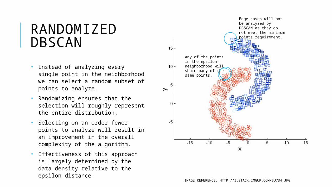
Image Reference: http://i.stack.imgur.com/Su734.jpg

RANDOMIZED DBSCAN

• Instead of analyzing every single point in the neighborhood we can select a random subset of points to analyze.

• Randomizing ensures that the selection will roughly represent the entire distribution.

• Selecting on an order fewer points to analyze will result in an improvement in the overall complexity of the algorithm.

• Effectiveness of this approach is largely determined by the data density relative to the epsilon distance.

Edge cases will not be analyzed by DBSCAN as they do not meet the minimum points requirement.

Any of the points in the epsilon-neighborhood will share many of the same points.

ALGORITHMexpandCluster(P, NeighborPts, C, eps, MinPts, k)

add P to cluster C

for each point P' in NeighborPts

if P' is not visited

mark P' as visited

NeighborPts' = regionQuery(P', eps)

if sizeof(NeighborPts') >= MinPts

NeighborPts’ = maximumCoercion(NeighbotPts’, k)

NeighborPts = NeighborPts joined with NeighborPts'

if P' is not yet member of any cluster

add P' to cluster C

maximumCoercion(Pts, k)

visited <- number of visited points in Pts

points <- select max(sizeof(Pts) – k – visited, 0) elements from Pts

for each point P’ in points

mark P’ as visited

return Pts

The algorithm is the same as DBSCAN with a slight modification.

We force a maximum number of points to continue analysis. If there are more points in the neighborhood than the maximum then we mark them as visited.

Marking points as visited allows us to “skip” them by not performing a region query for those points.

This effectively reduces the overall complexity.

PROBABILISTIC ANALYSIS

For now, assume uniform distribution and two dimensions.

The probability of selecting a point distance d from the reference point is defined as

The probability increases as d increases.

𝜖2𝜖

PROBABILISTIC ANALYSIS

The probability of finding a point in the 2-epsilon shell given a k-point at distance d is defined as

This is from a modified lens equation

Divided by the area of the 2-epsilon shell

This can be approximated (from Vesica Piscis) as

𝜖2𝜖

PROBABILISTIC ANALYSIS

This probability is greater than zero for all d greater than zero. So long as a point exists between the reference point and epsilon then there is a chance that it will find the target point in the 2-epsilon shell.

This is the probability for finding a single point in the 2-epsilon shell. For each additional point in the shell the probability increases for finding any point.

𝜖2𝜖

COMPLEXITY

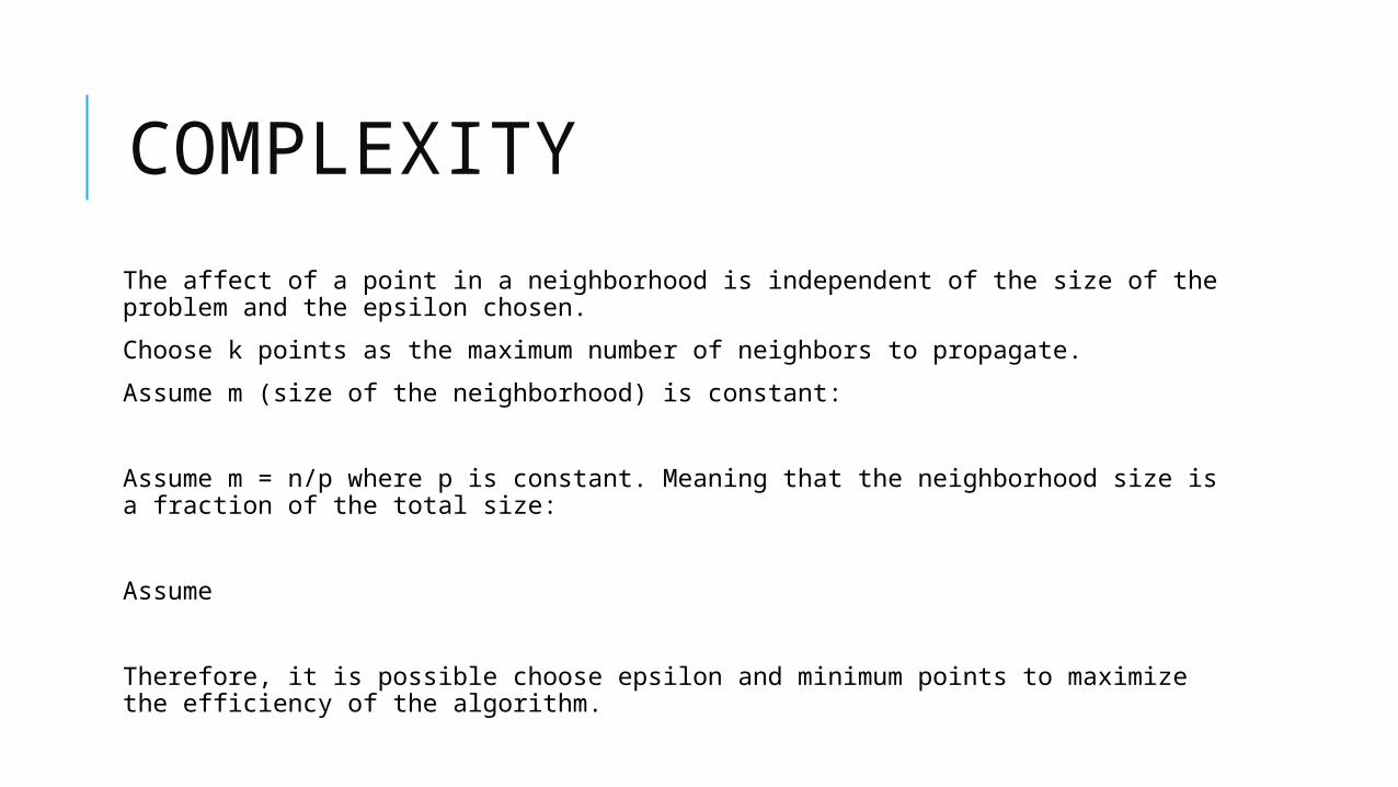
The affect of a point in a neighborhood is independent of the size of the problem and the epsilon chosen.

Choose k points as the maximum number of neighbors to propagate.

Assume m (size of the neighborhood) is constant:

Assume m = n/p where p is constant. Meaning that the neighborhood size is a fraction of the total size:

Assume

Therefore, it is possible choose epsilon and minimum points to maximize the efficiency of the algorithm.

COMPLEXITY

Choosing epsilon and minimum points such that the average number of points in a neighborhood is the square root of the number of points in the universe allows us to reduce the time complexity of the problem from to .

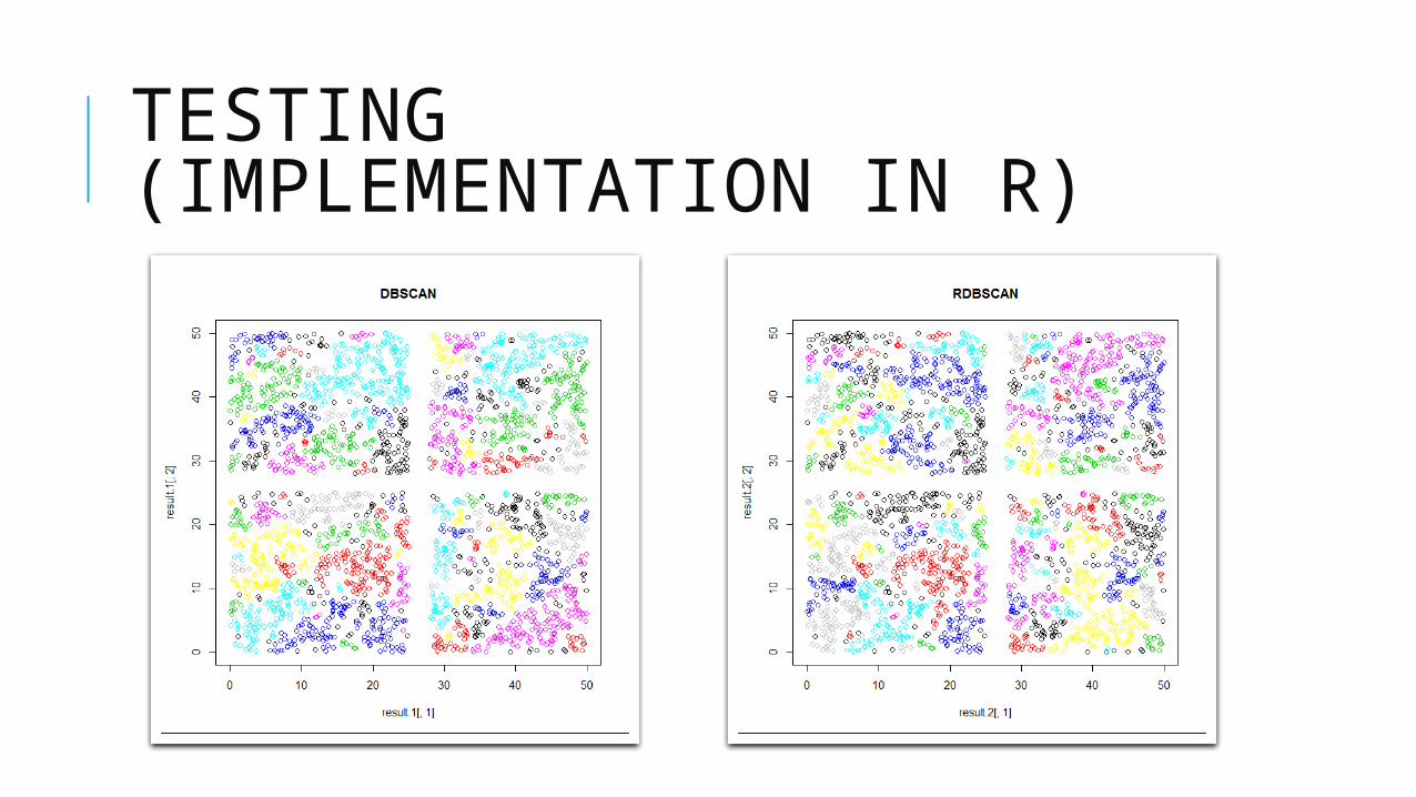
TESTING(IMPLEMENTATION IN R)

TESTING

Method

Generate a random data set of n elements with values ranging between 0 and 50. Then trim values between 25 and 25+epsilon on the x and y axis. This should give us at least 4 clusters.

Run the each algorithm 100 times on each data set and record the average running time for each algorithm and the average accuracy of Randomized DBSCAN.

Repeat for 1000, 2000, 3000, 4000 initial points (before trim)

Repeat for eps = [1:10]

500

1,00

0

1,50

0

2,00

0

2,50

0

3,00

0

3,50

0

4,00

0

4,50

00

5

10

15

20

25

30

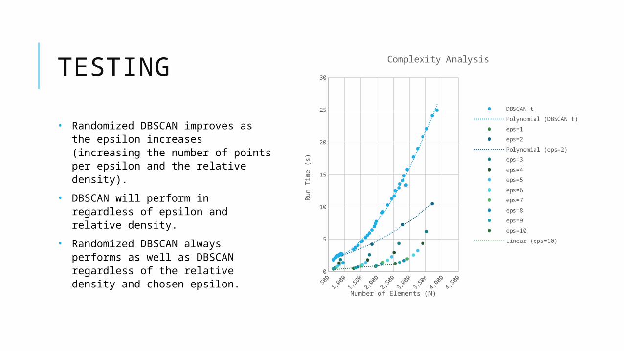
Complexity Analysis

DBSCAN t

Polynomial (DBSCAN t)

eps=1

eps=2

Polynomial (eps=2)

eps=3

eps=4

eps=5

eps=6

eps=7

eps=8

eps=9

eps=10

Linear (eps=10)

Number of Elements (N)

Run T

ime (

s)

TESTING

• Randomized DBSCAN improves as the epsilon increases (increasing the number of points per epsilon and the relative density).

• DBSCAN will perform in regardless of epsilon and relative density.

• Randomized DBSCAN always performs as well as DBSCAN regardless of the relative density and chosen epsilon.

500

1,00

0

1,50

0

2,00

0

2,50

0

3,00

0

3,50

0

4,00

0

4,50

00

5

10

15

20

25

30

Complexity Analysis

DBSCAN t

Polynomial (DBSCAN t)

eps=1

eps=2

Polynomial (eps=2)

eps=3

eps=4

eps=5

eps=6

eps=7

eps=8

eps=9

eps=10

Linear (eps=10)

Number of Elements (N)

Run T

ime (

s)

TESTING

• Running time is dependent upon number of elements; however, it improves with higher relative densities.

• Even a large amount of data can be processed quickly with a high relative density.

0 20 40 60 80 100 120 140 160 1800

5

10

15

20

25

957

921877

835835785764711662 665

1,918

1,845

1,7661,709

1,6481,5501,5181,4161,344 1,284

2,890

2,797

2,672

2,5252,448

2,322 2,179 2,156 1,973 1,954

3,840

3,696

3,528

3,409

3,2503,117

2,928 2,833 2,694 2,557

f(x) = 5.20116481731379 x^-0.363622868489098

Complexity Analysis

Points Per Epsilon (PPE)

Runnin

g T

ime (

s)

TESTING

• For any relative density above the minimum points threshold the Randomized DBSCAN algorithm returns the exact same result as the DBSCAN algorithm.

• We would expect the Randomized DBSCAN to be more accurate at higher densities (higher probability for each point in epsilon range); however, it doesn’t seem to matter above a very small threshold.

0 20 40 60 80 100 120 140 160 1800

10

20

30

40

50

60

70

Accuracy Analysis

Points Per Epsilon (PPE)

Err

or

(%)

FUTURE WORK

• Probabilistic analysis to determine accuracy of the algorithm in n dimensions. Does the k-accuracy relationship scale linearly or (more likely) exponentially with the number of dimensions.

• Determine performance and accuracy implications for classification and discreet attributes.

• Combine the randomized DBSCAN with an indexed region query to reduce the time complexity of the clustering algorithm from to .

• Rerun tests with balanced data sets to highlight (and better represent) improvement.

• Determining optimal epsilon for performance and accuracy of a particular data set.

DBRS

A Density-based Spatial Clustering Method with Random Sampling Initially proposed by Xin Wang and Howard J. Hamilton in 2003 Randomly selects points and assigns clusters Merges clusters that should be together

Advantages Handles varying densities

Disadvantages Same time and space complexity limitations as DBSCAN Requires an additional parameter and accompanying concept: purity

REFERENCES

I. Ester, Martin; Kriegel, Hans-Peter; Sander, Jörg; Xu, Xiaowei (1996). "A density-based algorithm for discovering clusters in large spatial databases with noise". In Simoudis, Evangelos; Han, Jiawei; Fayyad, Usama M. "Proceedings of the Second International Conference on Knowledge Discovery and Data Mining (KDD-96)". AAAI Press. pp. 226–231. ISBN 1-57735-004-9. CiteSeerX: 10.1.1.71.1980.

II. Wang, Xin; Hamilton, Howard J. (2003) “DBRS: A Desity-Based Spatial Clustering Method with Random Sampling.”

III. Gareth James, Daniela Witten, Trevor Hastie and Robert Tibshirani, An Introduction to Statistical Learning: with Applications in R, Springer, 1st ed, 2013, ISBN: 978-1461471370

IV. Michael Mitzenmacher and Eli Upfal, Probability and Computing: Randomized Algorithms and Probabilistic Analysis, Cambridge University Press, 1st ed, 2005, ISBN: 978-0521835404

V. Weisstein, Eric W. "Lens." From MathWorld--A Wolfram Web Resource. http://mathworld.wolfram.com/Lens.html