Date: 2008/11/7

Complex Fluids & Molecular Rheology Laboratory, Department of Chemical Engineering,

National Chung Cheng University, Chia-Yi 621, Taiwan, R.O.C.

Speaker: C. C. Hua (華繼中 )

Single-Chain and Aggregation Properties in Semiconducting Conjugated Polymer Solutions

Rheo-Optical Measurements and Multiscale Simulation

成大化工演講

Introduction & motivation

Spin-coating

Castfilms

Ink-jet printing

Conducting conjugated polymer precursor solution

Real process

Flexible PLED display PLED display Polymer solar celle-Paper

Cambridge Display Technology (CDT)

LG.Philips LCD Co. Ltd.

Cambridge Display Technology (CDT)

Seiko Epson Corporation

Seiko Epson Corporation

Konarka Technologies, Inc. Scientific American Feb. 2004

Viscometric Properties of MEH-PPV Viscometric Properties of MEH-PPV SolutionsSolutions

1 / T

0.0028 0.0030 0.0032 0.0034 0.0036 0.0038

0 M

/cR

T(s

)

1e-6

1e-5

1e-4

chloroform, heatingchloroform, annealingtoluene, heatingtoluene, annealing

278288298308T (K)

318338348 328

Hua et al, J Rheol 49, 641 (2005)

Poly[2-methoxy-5-(2’-ethyl-hexyloxy)-1,4-phenylene vinylene](MEH-PPV) [Mw: 70,000-10,000 g/mol, PDI: 2.5]

Mw = 280,000 g / mol ; C=1.56 mg/mL

1 / T

0.00295 0.00300 0.00305 0.00310 0.00315 0.00320 0.00325 0.00330 0.00335

p M

/cR

T(s

)

1e-8

1e-7

1e-6

1e-5

heatingannealing

Time (hr)

0 200 400 600 800

p/c

(cP

*ml/m

g)

0.00

0.05

0.10

0.15

0.20

0.25

0.30

0.35

0.40

chloroform (40oC)toluene (40oC)toluene (25oC)

Mw=280,000 g / mol , T= 318K

Time (hrs)

20 40 60 80 100 120 140 160 180 200 220 240

p/c(

cP*m

L/m

g)

0.00

0.01

0.02

0.03

0.04

0.546 mg/mL0.780 mg/mL2.344 mg/mL

MEH-PPV PSA. Effect of aging

B. Effect of thermal annealing

Dynamic Light Scattering (DLS)/Photoluminescence (PL): Effects of solvent quality and concentration

(s)

100 101 102 103 104 105 106

g(1

) ()

0.0

0.2

0.4

0.6

0.8

1.0

shear no shear shear (with filtration) no shear (with filtration)

(s)

100 101 102 103 104 105

g(1) (

)0.0

0.2

0.4

0.6

0.8

1.0

shear no shear

time (s)

1e+0 1e+1 1e+2 1e+3 1e+4 1e+5 1e+6

g(1) (

)

0.0

0.2

0.4

0.6

0.8

1.0

shearno shear

M/T: 1 mg/ml M/T: 3 mg/ml, no filtration M/C: 3 mg/ml, no filtration

wavelength (nm)

550 600 650 700 750 800

inte

nsi

ty (

a.u

.)

0

20

40

60

80

10 mg/ml (shear)10 mg/ml (no shear) 5 mg/ml (shear)5 mg/ml (no shear) 3 mg/ml (shear) 3 mg/ml (no shear)1 mg/ml (shear) 1 mg/ml (no shear)

wavelength (nm)

550 600 650 700 750 800

inte

nsi

ty (

a.u

.)

0

20

40

60

80

1mgml (shear) 1mgml (no shear) 3mgml (shear)3mgml (no shear) 5mgml (shear) 5mgml (no shear) 10mgml (shear) 10mgml (no shear)

M/T M/CHua et al., Appl. Phys. Lett. 93, 123303 (2008)

In situ viscometirc/flow turbidity measuring apparatus

Mechanical measuring system

Temperature control system

Optical measuring system

Specific turbidity measuring theory

1ln (1)

: transmittance

: the path length of light passed through the sample

T TL

T

L

(2)

: number of scattering centers

: total light energy scattered by one sphere

T sca

sca

NC

N

C

2

2

Using Mie theory and assumed spherical scattering

centers to simply analysis

(3)

: scattering efficiency

: Mie radius

2

sca sca

sca

sca

C Q a

Q

a

Q

2 2

1

2 1 (4)i ii

i a b

Derived specific turbidity representation equation

1

1

2

1

: Ricatti-Bessel function

: Hankel function

2

: wave length of incident light

: refractive index of sca

i i i ii

i i i i

i n i ii

i i i i

i

i

m m ma

m m m

m m mb

m m m

x

x

n a

nm

n

n

2

ttering center

: refractive index of mediumn

Kerker, M., THE SCATTERIG OF LIGHT AND OTHER ELECTROMAGNETIC RADIATION (Academic Press, San Diego, 1969).

van de Hulst, H. C., Light Scattering by Small Particles (Dover Publications, New York, 1981).

Specific turbidity measuring theory

3 (5)

2

: specific turbidity

: density of scattering sphere

: concentration

scaT

T

Q

c

c

c

Heller, W., and W. J. Pangonis, “Theoretical Investigations on the Light Scattering of Colloidal Spheres. I. The Specific Turbidity,” J. Chem. Phys. 26, 498-506 (1957).

Liberatore, M. W., and A. J. McHugh, “Dynamics of shear-induced structure formation in high molecular weight aqueous solutions,” J. Non-Newton. Fluid 132, 45-52 (2005).

Plot figure of specific turbidity vs. Mie radius

Equation of fitting curve:

10.7588 32.30470.0687

0.3024 42.0251: specific turbidity

: Mie radius

x xy x

x xx

y

So, quantity of Mie radius can get from equation of fitting curve.

2 2

21

1

1

2

22 1

: Ricatti-Bessel function

: Hankel function

2

: wave length of incident l

sca i ii

i i i ii

i i i i

i n i ii

i i i i

i

i

Q i a b

m m ma

m m m

m m mb

m m m

x

x

n a

nm

n

1

2

ight

: refractive index of scattering center

: refractive index of medium

n

n

Experiment design and procedure

DLSIn-situ viscometirc/flow turbidity measurement

Use DLS to measure hydrodynamic radius.

Compared the value with the Mie radius from turbidity measurement.

Shear flow: 10 min

Shear rate: 60 [s-1]

Flow rested 15 min

Shear flow: 10 min

Shear rate: 151~2,800 [s-1]

Flow rested 15 min

Altered shear rate

Shear flow: 10 min

Shear rate: 60 [s-1]

Flow rested 15 min

Shear flow: 10 min

Shear rate: 151~2,800 [s-1]

Flow rested 15 min

Ru

n2R

un1

Altered shear rate

MEH-PPV/DOP Sample

The main idea is to change polymer conc. and aging time to observe their effects on aggregation properties.

Conc. [mg/ml]

0.02 0.3 1.0 3.0

Aging time

W/o aging 2-days aging

Experiment factors setting

Run1 is to observe the effect of flow shearing and cessation.

Run2 is to further study the effect of preshearing.

Specific turbidity signal (w/o aging)0.02 mg/ml 0.3 mg/ml 1.0 mg/ml 3.0 mg/ml

Page 07

Before shear

Before shear

Before shear

Before shear

Before shear

Before shear

1.0 mg/ml1.0 mg/ml (2-days aging) 3.0 mg/ml1.0 mg/ml (w/o aging)0.3 mg/ml0.3 mg/ml (2-days aging)0.02 mg/ml0.3 mg/ml (w/o aging)

Specific turbidity signal (2-days aging)

Before shear

Before shear

Before shear

Before shear

Before shear

Before shear

Turbidity measurement vs. viscosity measurementMie radius

w/o aging w/o aging

Close correlation was generally noted between these two measurements

The Mie radius and reduced viscosity decreases with increased polymer concentration.

Preshearing effect was quite obvious at lower concentrations

Reduced viscosity

Turbidity measurement vs. DLS measurement

Aging effect Conc.Mie radius Hydrodynamic radius

Before shearing Before shearing

W/o aging

0.02 mg/ml 106.58 205.64

0.3 mg/ml 54.87 62.40

1.0 mg/ml 53.05 58.33

3.0 mg/ml 44.92 56.34

Aged 2 days

0.02 mg/ml 118.13 225.74

0.3 mg/ml 57.42 63.46

1.0 mg/ml 50.85 52.32

3.0 mg/ml 45.51 51.12

Except for the case with the lowest concentration, good agreement was found between the two measurements for the estimated aggregate size.

Ongoing work on rheo-optical measuring systems

Lenstra, T. A. J., Colloids near phase transition lines under shear, Doctoral thesis, Utrecht University, 2001.

Flow/turbidity Dicroism & birefringence

SALS & multi-angle LS Wide range of rheo-optical measurement

Kume et al., Macromolecules 30, 7232-7236 (1997).

Anton Paar

SALS Multi-angle LS

Ongoing work by Liu, Wen, and Kuo.

Ongoing work by Chen.

Page 15

Multi-Angle Dynamic/Static Light Scattering

Sample cell Photomultiplier tube

TemperatureController10~70oC

θ = 30~150o

Polarizer 1Polarizer 2

Circulating water

Detection arm

Small Angle Light Scattering (SALS)

CCD

Photodiode 1

Photodiode 2

θ = 0.5~10o

Sample cell

CCDLaser

Spatial filter Mini rod mirror

2 mm

Objectivelens

Pinhole

Lens

Iris

Beamsplitter

Photodiode 1

Sample cell

Lens set 1 Lens set 2

Photodiode 2

Iris

DAQ

SchematicDiagram ofSALS Setup

OnsetEdmund

Ray tracing

Rheo-Turbidity

Optical cellOptical cell

Thermal bathThermal bath

PhotodiodePhotodiode

Photodiode 1

Photodiode 2

Rheometer

TemperatureController

Opticalflowcell

Couette flow cell

Polarizer 2 at 135o

Polarizer 1 at 45o

Photodiode 2

Photodiode 1

Rheometer

Flow Birefringence (Crossed Polarizers)

He-Ne laser

Flow Light Scattering (FLS)

Lens A

Laser

Pinhole A

Iris

Lens B

Pinhole B

Det

ecto

r

Index matching vat

Rotor

Data analysis

Rotary detection arm (top view)Rotary detection arm (top view)

30336066

30

153

16.55 8

3

1.5

37

3

37

60

66

33

30

Optical flow cell for FLSOptical flow cell for FLS

主要量測系統 : (1) 即時光學—流變系統

I. Particle Interactions II. Microstructures III. Molecular Anisotropy

主要量測系統 : (2) 光學旋轉塗佈成膜系統

Video MicroscopyLaser Doppler, DLS

I. Ellipsometry (film thickness & reflective index) II. Aggregation Microstructure/Anisotropy & Hydrodynamics under controlled (a) Solution Properties (solvent quality, volume fraction, viscosity & volatility) (b) Spin Rate (c) Baking (d) Interfacial Properties

Fundamental Particle(Polymer segment)

Interactions

Small Aggregates

Self-assembly/Phase separation

Microscopic/MesoscopicStructure &Anisotropy

Particle size, shape,Surface modifications, (grafting & charge)

Solution properties (solvent quality, concentration, viscosity, volatility)

Interfacial properties (wetting & brushing)

Operating Conditions (spin rate,evaporationviscoelasticity)

Optoelectronic/ Mechanical Properties

X-ray Scattering

DynamicLight scattering

Molecular Rheology

Static light scattering &Birefringence/Dichroism Video Microscopy

Spectroscopy(EL & PL etc),TEM, AFM etc.

Non-Equilibrium & Memory Effects

Parameter-FreeParameter-Free MultiscaleMultiscale Coarse-Grained (CG) Simulations Coarse-Grained (CG) Simulations

SystemNo. of chains/

in monomer unitNo. of solvent particles

Density（ g/cm3）

Concentration（ wt %）

(a)(b)(c)

MEH-PPV (n=100) × 11MEH-PPV (n=100) × 11

PS (n=100) × 11

Chloroform × 8000Toluene × 8000

Cyclohexane × 8000

1.210.980.84

22.9127.8014.58

(c)

Aggregates versus Entanglements

Temperature ＝ 55 ˚C, Pressure ＝ 1 atm, Time ＝ 1 ns, Time step = 10 fs

Y-Z plane

Y-X planeX-Z plane

Y-Z plane

Y-X planeX-Z plane

(a) (b)

Hua et al, J Rheol 49, 641 (2005)

Automatic mappings and Langevin Dynamics Automatic mappings and Langevin Dynamics Simulations:Simulations:

Bond angle Planar angle

Distances between non-adjacent beads (Angstrom)

0 2 4 6 8 10 12 14 16 18

RD

F (

prob

abili

ty);

Ene

rgy

(kca

l/mol

)

-0.4

0.0

0.4

0.8

1.2

1.6

2.0

2.4

MD simulationCGMD simulationCG model with Lennard-Jones potential function

Distances between non-adjacent beads (Angstrom)

0 2 4 6 8 10 12 14 16 18

RD

F (

prob

abili

ty);

Ene

rgy

(kca

l/mol

)

-0.4

0.0

0.4

0.8

1.2

1.6

2.0

2.4

MD simulationCGMD simulationCG model with Lennard-Jones potential function

Distances between non-adjacent beads (Angstrom)

0 2 4 6 8 10 12 14 16 18

RD

F (

prob

abili

ty);

Ene

rgy

(kca

l/mol

)

-0.3

0.0

0.3

0.6

0.9

1.2

1.5

1.8

MD simulationCG model with Lennard-Jones potential functionCGMD simulation

Force-Fields Construction for the CG-model Lee, C. K.; Hua, C. C.; Chen, S. A. J. Phys. Chem. B 112, 11479 (2008).

Bond length

Toluene vs Toluene Chloroform vs Chloroform Monomer vs Monomer

Intr

amo

lecu

lar

Inte

rmo

lecu

lar

O

O O

OO

OO

OO

O O

O

Distance between two adjacent beads (Angstrom)

1 2 3 4 5 6 7 8 9 10

Pro

babi

lity

0.00

0.03

0.06

0.09

0.12

0.15

MD dataCGMD data

Angle between three successive beads (radians)

0.0 0.5 1.0 1.5 2.0 2.5 3.0

Pro

babi

lity

0.00

0.03

0.06

0.09

0.12

MD dataCGMD data

Planar angle between four successive beads (radians)

0 1 2 3 4 5 6

Pro

ba

bili

ty

0.000

0.008

0.016

0.024

0.032

0.040

MD dataCGMD data

Distance between two adjacent beads (Angstrom)

1 2 3 4 5 6 7 8 9 10

En

erg

y (k

cal/m

ol)

0.7

1.4

2.1

2.8

3.5

4.2

MD dataTwo Gaussian potential functions

Angle between three successive beads (radians)

0.0 0.5 1.0 1.5 2.0 2.5 3.0

En

erg

y (k

cal/m

ol)

0.8

1.6

2.4

3.2

4.0

4.8

MD dataOne Gaussian potential function

Planar angle between four successive beads (radians)

0 1 2 3 4 5 6

En

erg

y (k

cal/m

ol)

1.6

2.4

3.2

4.0

4.8

5.6

MD dataFourier progression functions

Parameter-FreeParameter-Free, Self-consistent Langevin Dynamics of the CG-Model:, Self-consistent Langevin Dynamics of the CG-Model:

M / T6 ns

M / C6 ns

2

2i i

i i ij ij

d dm

dtdt r r

F ξ B /i ik T D from the MD simulation of single-particle diffusivities

CGMD : Parallel computation system (IBM-P690 with 4 CPUs) with 36 hrs

CGLD : Single-CPU personal with 10 min

Which yields the exact (generally poor) solvent qualities for MEH-PPV solutions:Toluene: 0.32 Chloroform: 0.38

log N

1.9 2.0 2.1 2.2 2.3 2.4 2.5 2.6 2.7 2.8

log

R

1.2

1.4

1.6

1.8

2.0

2.2

2.4

MEH-PPV / Toluene MEH-PPV / Chloroform

log log log

0.32 0.02, 1.07 0.05

0.38 0.01, 1.07 0.03

R a N b

a b

a b

Scaling behavior of the mean end-to-end distance:

No. of MEH-PPV (m )ono : 100 ~ 500mers N

g,MT

p,MT

11 2G, MT

34.4 0.7 (A)

65.1 11.8 (A)

7.51 10 (m /s)

R

L

D

g,MC

p,MC

11 2G, MC

43.7 0.5 (A)

73.3 12.5 (A)

9.62 10 (m /s)

R

L

D

50 MEH-PPV monomersper Kuhn length

M / T0.5 ns

Nucleation of two small aggregatesNucleation of two small aggregates Collapsing of ten MEH-PPV chainsCollapsing of ten MEH-PPV chains into an aggregate clusterinto an aggregate cluster

M / C0.38 ns

M / T7.5 ns

M / T0.38 ns M / T

0.38 nsM / T0.38 ns

M / C7.5 ns

M / C7.5 ns

3N,MC

g,MC

0.9 (

54.3 (A)

bead/nm )

R

3N,MT

g,MT

2.0 (

41.6 (A)

bead/nm )

R

3N,MT

g,MT

0.7 (

70.4 (A)

bead/nm )

R

3N,MC

g,MC

0.4 (

86.8 (A)

bead/nm )

R

M/T0.8 ns

M/T8 ns

M/C 0.8 ns

M/C 8 ns

M/T 0.8 ns

M/T 8 ns

M/C0.8 ns

M/C8 ns

Brownian Dynamics of Chain ModelsBrownian Dynamics of Chain Models

SolventMolecular

weight (Da) Number of

monomers, Nm

Size of monomer, bm (nm) a

<R2>end-to-end, (nm2) a,b

Solvent quality, a,c

Chloroform 80000 300 0.55 54.76 0.38

Toluene 80000 300 0.55 30.25 0.32

Basic information of MEH-PPV Chains in solvents at 298K:

aEstimated from atomic molecular dynamics simulations. bThe mean-square end-to-end distance. cBased on <R2>end-to-end = K(Nm-1)2, where K is a certain constant independent of the polymer molecular weight.

LKuhn (=17.5 nm): the Kuhn lengthh* (= 0.25): hydrodynamic interactions parameterf: total volume fraction of monomer as polymer chain in a solventRg,: radius of gyration of a FJC (or FRC) under the -condition(=LKuhn

2/(12kBT)): relaxation time of the Kuhn segment, where , kB and T are the drag coefficient, the Boltzmann constant and absolute temperature

Effects of coarse-grained level & bead size

/ (kBT)

0.0 0.5 1.0 1.5 2.0

<R

2 >en

d-to

-end

/ L

Kuh

n2

1

2

3

4

5

6

7

FRC, /Qeq = 1

h/Qeq = 2/3

FJC, h/Qeq = 2/3

*

21stretch

1 eq1

22bend

1/3* 3eq ,

eq1

12 62

LJ

2

m eq

B eq Kuhn

1

2

1

2

4

,

/

1000 , 1.

8 / 3 8 /

Freely jointed chain :

Fr

50

e

N

i ii

N

ii

N N

i j i j i j

gh

i

U H Q

U H

U

Q

H k T Q

h Q f N

L

R

N

r r

r r r r

m eq

B eq Kuhn B eq

/

2142 , 0.2 , 14 , 0.

ely rotat 1ing chain :0Q

H k T Q L H k T

N

The values chosen for H and H produce a<R2>end-to-end of FRC/FJC in agreement with the predicted ideal chain behavior.

FRC (freely rotating chain)

FJC (freely jointed chain)

The value of for a given polymer solution canin princinple be determined from the polymer collapsed transition shown above.

0

5

10

15

20

25

510

1520

250

5

10

15

20

25

Z

X

Y

MEH-PPV/Chloroform, t / = 10000

Aggregation in MEH-PPV Solutions: Freely Jointed Chain ModelAggregation in MEH-PPV Solutions: Freely Jointed Chain Model

0

5

10

15

20

25

510

1520

250

5

10

15

20

25

Z

X

Y

t / = 0

0

5

10

15

20

25

510

1520

250

5

10

15

20

25

Z

X

Y

MEH-PPV/Toluene, t / = 10000

0

5

10

15

20

25

0

5

10

15

20

25

05

1015

20

Z

X

Y

t / = 0

chain bead eq box Kuhn eq Kuhn*, 7, / 2 / 3, / 25,1 / 100 hN N Q L L Q L

0

5

10

15

20

25

0

5

10

15

20

25

05

1015

20

Z

X

Y

MEH-PPV/Chloroform, t / = 10000

0

5

10

15

20

25

0

5

10

15

20

25

05

1015

20

Z

X

Y

MEH-PPV/Toluene, t / = 10000Case I

Case II

Scattering of Single Collapsed Chains/interchain aggregates predicted by Scattering of Single Collapsed Chains/interchain aggregates predicted by Freely Rotating Chain ModelFreely Rotating Chain Model

SANS profiles of MEH-PPV in (a) chloroform and (b) toluene at 25 °C. Mn = 216,000 g/mol and PDI = 2.0.(Ou-Yang et al., Phys. Rev. E 72, 031802 (2005))

(b)(a)

local rod-like feature of MEH-PPV molecules

qLKuhn > 5, rod-like

1<qLKuhn<5, fractal structure

To retrieve pure MEH-PPV contributions from the SANS data, the scattering intensity is normalized as I(q)/()2, where is the difference of scattering length density betweenthe MEH-PPV monomer and the solvent molecule.

Effects of single-chain polydispersity and interchain aggregation

qLKuhn/(2)

0.1 1

<I(

q)>

/(

2 )

103

104

105

0.1 wt%, Chloroform TolueneSimulation, Chloroform Toluene

-1

(a) /Rseg = 1.37

qLKuhn/(2)

0.1 1

<I(

q)>

/(

2 )

103

104

105

0.1 wt%, Chloroform TolueneSimulation, Chloroform Toluene

S. C. Shie, C. C. Hua, and S. A. Chen, “Simulation of large-scale material properties of semiflexible chains in poor solvents” to be submitted.

Parameter determinations for even more coarse-grained, rigid dumbbell models:

From Freely joined chains to dumbbells

The right figure shows that the interchain potentialas a function of the separation in the mass centerscan be well mimicked by some linear functions

Solvent /Rs /(kT) rcut / [<R2>end-to-end]1/2

MEH-PPVChloroform 0.31 1.2 1.04

Toluene 0.28 2.2 0.94

PS -solvent 0.26 0.5 1.23

Parameter evaluations for the dumbbell:

612

chain, 4

ijij

jiUrrrr

.,

,,

,,

cut

cutcutcut

12

dumbbell,

r

rrr

U

ij

ijij

ijij

ji

rr0

rrrr

rrrr

Shie et al. Macroml. Theory. & Simul. 16, 117 (2007)

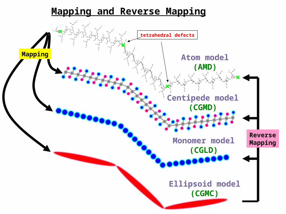
Mapping and Reverse Mapping

Atom model(AMD)

Monomer model(CGLD)

Ellipsoid model(CGMC)

tetrahedral defects

Centipede model(CGMD)

Mapping

ReverseMapping