Database System Architectures

Dr.Mahesh R Sanghavi

Unit 4

Database System Architectures

• Centralized and Client-Server Systems

• Server System Architectures

• Parallel Systems

• Distributed Systems

• Network Types

Centralized Systems

• Run on a single computer system and do not interact with other computer systems.

• General-purpose computer system: one to a few CPUs and a number of device controllers that are connected through a common bus that provides access to shared memory.

• Single-user system (e.g., personal computer or workstation): desk-top unit, single user, usually has only one CPU and one or two hard disks; the OS may support only one user.

• Multi-user system: more disks, more memory, multiple CPUs, and a multi-user OS. Serve a large number of users who are connected to the system vie terminals. Often called server systems.

A Centralized Computer System

Client-Server Systems

• Server systems satisfy requests generated at mclient systems, whose general structure is shown below:

Client-Server Systems • Database functionality can be divided into:

– Back-end: manages access structures, query evaluation and optimization, concurrency control and recovery.

– Front-end: consists of tools such as forms, report-writers, and graphical user interface facilities.

• The interface between the front-end and the back-end is through SQL or through an application program interface.

Client-Server Systems

• Advantages of replacing mainframes with networks of workstations or personal computers connected to back-end server machines:– better functionality for the cost– flexibility in locating resources and expanding

facilities– better user interfaces– easier maintenance

Server System Architecture

• Server systems can be broadly categorized into two kinds:

– transaction servers which are widely used in relational database systems, and

– data servers, used in object-oriented database systems

Transaction Servers

• Also called query server systems or SQL server systems– Clients send requests to the server– Transactions are executed at the server– Results are shipped back to the client.

• Requests are specified in SQL, and communicated to the server through a remote procedure call (RPC) mechanism.

• Transactional RPC allows many RPC calls to form a transaction.

• Open Database Connectivity (ODBC) is a C language application program interface standard from Microsoft for connecting to a server, sending SQL requests, and receiving results.

• JDBC standard is similar to ODBC, for Java

Transaction Server Process Structure

• A typical transaction server consists of multiple processes accessing data in shared memory.

• Server processes– These receive user queries (transactions), execute them

and send results back– Processes may be multithreaded, allowing a single process

to execute several user queries concurrently– Typically multiple multithreaded server processes

• Lock manager process

• Database writer process– Output modified buffer blocks to disks continually

Transaction Server Processes (Cont.)

• Log writer process– Server processes simply add log records to log record

buffer

– Log writer process outputs log records to stable storage.

• Checkpoint process– Performs periodic checkpoints

• Process monitor process– Monitors other processes, and takes recovery actions

if any of the other processes fail• E.g. aborting any transactions being executed by a server

process and restarting it

Transaction System Processes (Cont.)

Transaction System Processes (Cont.)

• Shared memory contains shared data – Buffer pool– Lock table– Log buffer– Cached query plans (reused if same query submitted

again)• All database processes can access shared memory• To ensure that no two processes are accessing the

same data structure at the same time, databases systems implement mutual exclusion using either– Operating system semaphores– Atomic instructions such as test-and-set

• To avoid overhead of interprocess communication for lock request/grant, each database process operates directly on the lock table – instead of sending requests to lock manager process

• Lock manager process still used for deadlock detection

Data Servers• Used in high-speed LANs, in cases where

– The clients are comparable in processing power to the server– The tasks to be executed are compute intensive.

• Data are shipped to clients where processing is performed, and then shipped results back to the server.

• This architecture requires full back-end functionality at the clients.

• Used in many object-oriented database systems • Issues:

– Page-Shipping versus Item-Shipping– Locking– Data Caching– Lock Caching

Data Servers (Cont.)

• Page-shipping versus item-shipping– Smaller unit of shipping more messages– Worth prefetching related items along with requested item– Page shipping can be thought of as a form of prefetching

• Locking– Overhead of requesting and getting locks from server is high

due to message delays– Can grant locks on requested and prefetched items; with

page shipping, transaction is granted lock on whole page.– Locks on a prefetched item can be P{called back} by the

server, and returned by client transaction if the prefetcheditem has not been used.

– Locks on the page can be deescalated to locks on items in the page when there are lock conflicts. Locks on unused items can then be returned to server.

Data Servers (Cont.)

• Data Caching– Data can be cached at client even in between transactions– But check that data is up-to-date before it is used (cache

coherency)– Check can be done when requesting lock on data item

• Lock Caching– Locks can be retained by client system even in between

transactions– Transactions can acquire cached locks locally, without

contacting server– Server calls back locks from clients when it receives conflicting

lock request. Client returns lock once no local transaction is using it.

– Similar to deescalation, but across transactions.

Parallel Systems

• Parallel database systems consist of multiple processors and multiple disks connected by a fast interconnection network.

• A coarse-grain parallel machine consists of a small number of powerful processors

• A massively parallel or fine grain parallel machine utilizes thousands of smaller processors.

• Two main performance measures:– throughput --- the number of tasks that can be completed

in a given time interval

– response time --- the amount of time it takes to complete a single task from the time it is submitted

Speed-Up and Scale-Up• Speedup: a fixed-sized problem executing on a small

system is given to a system which is N-times larger.– Measured by:speedup = small system elapsed time

large system elapsed time– Speedup is linear if equation equals N.

• Scaleup: increase the size of both the problem and the system– N-times larger system used to perform N-times larger job– Measured by:scaleup = small system small problem elapsed time

big system big problem elapsed time – Scale up is linear if equation equals 1.

Speedup

Speedup

Scaleup

Scaleup

Batch and Transaction Scaleup• Batch scaleup:

– A single large job; typical of most decision support queries and scientific simulation.

– Use an N-times larger computer on N-times larger problem.

• Transaction scaleup:– Numerous small queries submitted by independent

users to a shared database; typical transaction processing and timesharing systems.

– N-times as many users submitting requests (hence, N-times as many requests) to an N-times larger database, on an N-times larger computer.

– Well-suited to parallel execution.

Factors Limiting Speedup and Scaleup

Speedup and scaleup are often sublinear due to:• Startup costs: Cost of starting up multiple

processes may dominate computation time, if the degree of parallelism is high.

• Interference: Processes accessing shared resources (e.g.,system bus, disks, or locks) compete with each other, thus spending time waiting on other processes, rather than performing useful work.

• Skew: Increasing the degree of parallelism increases the variance in service times of parallely executing tasks. Overall execution time determined by slowest of parallely executing tasks.

Interconnection Network Architectures

• Bus. System components send data on and receive data from a single communication bus;– Does not scale well with increasing parallelism.

• Mesh. Components are arranged as nodes in a grid, and each component is connected to all adjacent components– Communication links grow with growing number of

components, and so scales better. – But may require 2 n hops to send message to a node (or n

with wraparound connections at edge of grid).• Hypercube. Components are numbered in binary;

components are connected to one another if their binary representations differ in exactly one bit.– n components are connected to log(n) other components

and can reach each other via at most log(n) links; reduces communication delays.

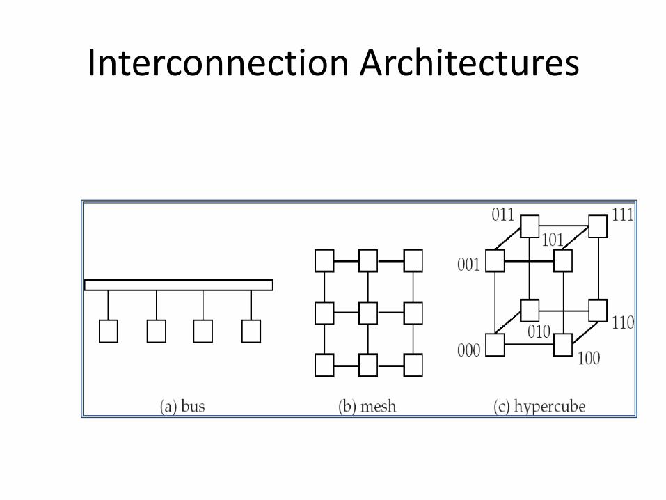
Interconnection Architectures

Parallel Database Architectures

• Shared memory -- processors share a common memory

• Shared disk -- processors share a common disk

• Shared nothing -- processors share neither a common memory nor common disk

• Hierarchical -- hybrid of the above architectures

Parallel Database Architectures

Shared Memory

• Processors and disks have access to a common memory, typically via a bus or through an interconnection network.

• Extremely efficient communication between processors —data in shared memory can be accessed by any processor without having to move it using software.

• Downside – architecture is not scalable beyond 32 or 64 processors since the bus or the interconnection network becomes a bottleneck

• Widely used for lower degrees of parallelism (4 to 8).

Shared Disk• All processors can directly access all disks via an interconnection

network, but the processors have private memories.– The memory bus is not a bottleneck– Architecture provides a degree of fault-tolerance — if a processor

fails, the other processors can take over its tasks since the database is resident on disks that are accessible from all processors.

• Examples: IBM Sysplex and DEC clusters (now part of Compaq) running Rdb (now Oracle Rdb) were early commercial users

• Downside: bottleneck now occurs at interconnection to the disk subsystem.

• Shared-disk systems can scale to a somewhat larger number of processors, but communication between processors is slower.

Shared Nothing• Node consists of a processor, memory, and one or more disks.

Processors at one node communicate with another processor at another node using an interconnection network. A node functions as the server for the data on the disk or disks the node owns.

• Examples: Teradata, Tandem, Oracle-n CUBE• Data accessed from local disks (and local memory accesses)

do not pass through interconnection network, thereby minimizing the interference of resource sharing.

• Shared-nothing multiprocessors can be scaled up to thousands of processors without interference.

• Main drawback: cost of communication and non-local disk access; sending data involves software interaction at both ends.

Hierarchical• Combines characteristics of shared-memory, shared-

disk, and shared-nothing architectures.• Top level is a shared-nothing architecture – nodes

connected by an interconnection network, and do not share disks or memory with each other.

• Each node of the system could be a shared-memory system with a few processors.

• Alternatively, each node could be a shared-disk system, and each of the systems sharing a set of disks could be a shared-memory system.

• Reduce the complexity of programming such systems by distributed virtual-memory architectures– Also called non-uniform memory architecture (NUMA)

Distributed Systems

• Data spread over multiple machines (also referred to as sites or nodes).

• Network interconnects the machines

• Data shared by users on multiple machines

Distributed Databases

• Homogeneous distributed databases– Same software/schema on all sites, data may be partitioned

among sites– Goal: provide a view of a single database, hiding details of

distribution• Heterogeneous distributed databases

– Different software/schema on different sites– Goal: integrate existing databases to provide useful

functionality• Differentiate between local and global transactions

– A local transaction accesses data in the single site at which the transaction was initiated.

– A global transaction either accesses data in a site different from the one at which the transaction was initiated or accesses data in several different sites.

Trade-offs in Distributed Systems• Sharing data – users at one site able to access

the data residing at some other sites.• Autonomy – each site is able to retain a

degree of control over data stored locally.• Higher system availability through

redundancy — data can be replicated at remote sites, and system can function even if a site fails.

• Disadvantage: added complexity required to ensure proper coordination among sites.– Software development cost.– Greater potential for bugs.– Increased processing overhead.

Implementation Issues for Distributed Databases

• Atomicity needed even for transactions that update data at multiple sites

• The two-phase commit protocol (2PC) is used to ensure atomicity– Basic idea: each site executes transaction until just before

commit, and the leaves final decision to a coordinator– Each site must follow decision of coordinator, even if there is a

failure while waiting for coordinators decision

• 2PC is not always appropriate: other transaction models based on persistent messaging, and workflows, are also used

• Distributed concurrency control (and deadlock detection) required

• Data items may be replicated to improve data availability

Network Types

• Local-area networks (LANs) – composed of processors that are distributed over small geographical areas, such as a single building or a few adjacent buildings.

• Wide-area networks (WANs) – composed of processors distributed over a large geographical area.

Networks Types (Cont.)

• WANs with continuous connection (e.g. the Internet) are needed for implementing distributed database systems

• Groupware applications such as Lotus notes can work on WANs with discontinuous connection:– Data is replicated.– Updates are propagated to replicas periodically.– Copies of data may be updated independently.– Non-serializable executions can thus result. Resolution

is application dependent.

End of Chapter

JNN

Parallel Databases

J.N.Nandimath

Parallel Databases

• Introduction

• I/O Parallelism

• Interquery Parallelism

• Intraquery Parallelism

• Intraoperation Parallelism

• Interoperation Parallelism

• Design of Parallel Systems

Introduction Parallel machines are becoming quite common and

affordable Prices of microprocessors, memory and disks have dropped

sharply Recent desktop computers feature multiple processors and this

trend is projected to accelerate

Databases are growing increasingly large large volumes of transaction data are collected and stored for

later analysis. multimedia objects like images are increasingly stored in

databases

Large-scale parallel database systems increasingly used for: storing large volumes of data processing time-consuming decision-support queries providing high throughput for transaction processing

Parallelism in Databases Data can be partitioned across multiple disks for parallel

I/O. Individual relational operations (e.g., sort, join,

aggregation) can be executed in parallel data can be partitioned and each processor can work

independently on its own partition.

Queries are expressed in high level language (SQL, translated to relational algebra) makes parallelization easier.

Different queries can be run in parallel with each other.Concurrency control takes care of conflicts.

Thus, databases naturally lend themselves to parallelism.

I/O Parallelism

Reduce the time required to retrieve relations from disk by partitioning the relations on multiple disks. Horizontal partitioning – tuples of a relation are divided among many

disks such that each tuple resides on one disk. Partitioning techniques (number of disks = n):

Round-robin: Send the ith tuple inserted in the relation to disk i mod n.

Hash partitioning: Choose one or more attributes as the partitioning attributes. Choose hash function h with range 0…n - 1 Let i denote result of hash function h applied to the partitioning

attribute value of a tuple. Send tuple to disk i.

I/O Parallelism (Cont.)

Partitioning techniques (cont.):Range partitioning: Choose an attribute as the partitioning attribute. A partitioning vector [vo, v1, ..., vn-2] is chosen. Let v be the partitioning attribute value of a tuple. Tuples

such that vi vi+1 go to disk I + 1. Tuples with v < v0 go to disk 0 and tuples with v vn-2 go to disk n-1.

E.g., with a partitioning vector [5,11], a tuple with partitioning attribute value of 2 will go to disk 0, a tuple with value 8 will go to disk 1, while a tuple with value 20 will go to disk2.

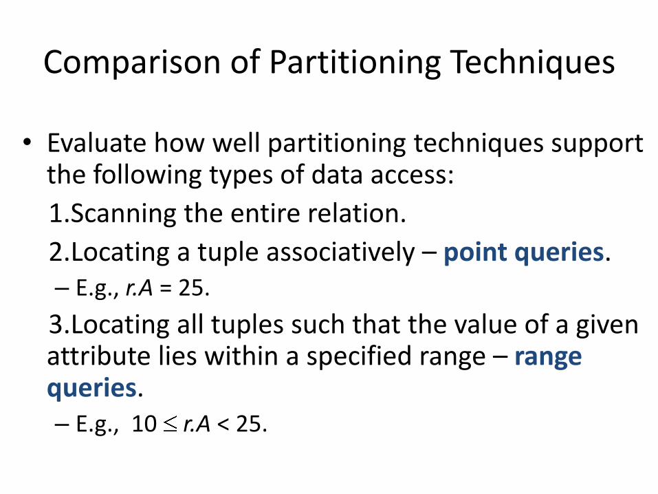
Comparison of Partitioning Techniques

• Evaluate how well partitioning techniques support the following types of data access:

1.Scanning the entire relation.

2.Locating a tuple associatively – point queries.– E.g., r.A = 25.

3.Locating all tuples such that the value of a given attribute lies within a specified range – range queries.– E.g., 10 r.A < 25.

Comparison of Partitioning Techniques (Cont.)

Round robin:Advantages Best suited for sequential scan of entire relation on

each query. All disks have almost an equal number of tuples;

retrieval work is thus well balanced between disks.

Range queries are difficult to processNo clustering -- tuples are scattered across all disks

Comparison of Partitioning Techniques(Cont.)

Hash partitioning: Good for sequential access Assuming hash function is good, and partitioning attributes

form a key, tuples will be equally distributed between disks Retrieval work is then well balanced between disks.

Good for point queries on partitioning attribute Can lookup single disk, leaving others available for

answering other queries. Index on partitioning attribute can be local to disk, making

lookup and update more efficient

No clustering, so difficult to answer range queries

Comparison of Partitioning Techniques (Cont.)

Range partitioning: Provides data clustering by partitioning attribute value. Good for sequential access Good for point queries on partitioning attribute: only one

disk needs to be accessed. For range queries on partitioning attribute, one to a few

disks may need to be accessed Remaining disks are available for other queries. Good if result tuples are from one to a few blocks. If many blocks are to be fetched, they are still fetched from one

to a few disks, and potential parallelism in disk access is wasted

Partitioning a Relation across Disks

• If a relation contains only a few tuples which will fit into a single disk block, then assign the relation to a single disk.

• Large relations are preferably partitioned across all the available disks.

• If a relation consists of m disk blocks and there are n disks available in the system, then the relation should be allocated min(m,n) disks.

Interquery Parallelism Queries/transactions execute in parallel with one another. Increases transaction throughput; used primarily to scale up a

transaction processing system to support a larger number of transactions per second.

Easiest form of parallelism to support, particularly in a shared-memory parallel database, because even sequential database systems support concurrent processing.

More complicated to implement on shared-disk or shared-nothing architectures Locking and logging must be coordinated by passing messages

between processors. Data in a local buffer may have been updated at another processor. Cache-coherency has to be maintained — reads and writes of data in

buffer must find latest version of data.

Cache Coherency Protocol

Example of a cache coherency protocol for shared disk systems: Before reading/writing to a page, the page must be locked in

shared/exclusive mode. On locking a page, the page must be read from disk Before unlocking a page, the page must be written to disk if it

was modified.

More complex protocols with fewer disk reads/writes exist. Cache coherency protocols for shared-nothing systems are

similar. Each database page is assigned a home processor. Requests to fetch the page or write it to disk are sent to the home processor.

Intraquery Parallelism

Execution of a single query in parallel on multiple processors/disks; important for speeding up long-running queries.

Two complementary forms of intraquery parallelism : Intraoperation Parallelism – parallelize the execution of each

individual operation like sort , select, project in the query. Interoperation Parallelism – execute the different operations in

a query expression in parallel.

the first form scales better with increasing parallelism becausethe number of tuples processed by each operation is typically more than the number of operations in a query

Parallel Processing of Relational OperationsIntraoperation Parallelism

Our discussion of parallel algorithms assumes: read-only queries shared-nothing architecture n processors, P0, ..., Pn-1, and n disks D0, ..., Dn-1, where

disk Di is associated with processor Pi.

If a processor has multiple disks they can simply simulate a single disk Di.

Shared-nothing architectures can be efficiently simulated on shared-memory and shared-disk systems. Algorithms for shared-nothing systems can thus be run

on shared-memory and shared-disk systems. However, some optimizations may be possible.

Parallel Sort

Intraoperation Parallelism1.Range-Partitioning Sort Choose processors P0, ..., Pm, where m n -1 to do sorting. Create range-partition vector with m entries, on the sorting attributes Redistribute the relation using range partitioning

all tuples that lie in the ith range are sent to processor Pi

Pi stores the tuples it received temporarily on disk Di. This step requires I/O and communication overhead.

Each processor Pi sorts its partition of the relation locally. Each processors executes same operation (sort) in parallel with other

processors, without any interaction with the others (data parallelism). Final merge operation is trivial: range-partitioning ensures that, for 1 j

m, the key values in processor Pi are all less than the key values in Pj.

Parallel Sort (Cont.)

2.Parallel External Sort-Merge• Assume the relation has already been partitioned among disks D0, ...,

Dn-1 (in whatever manner).• Each processor Pi locally sorts the data on disk Di.• The sorted runs on each processor are then merged to get the final

sorted output.• Parallelize the merging of sorted runs as follows:

– The sorted partitions at each processor Pi are range-partitioned across the processors P0, ..., Pm-1.

– Each processor Pi performs a merge on the streams as they are received, to get a single sorted run.

– The sorted runs on processors P0,..., Pm-1 are concatenated to get the final result.

Parallel Join

• The join operation requires pairs of tuples to be tested to see if they satisfy the join condition, and if they do, the pair is added to the join output.

• Parallel join algorithms attempt to split the pairs to be tested over several processors. Each processor then computes part of the join locally.

• In a final step, the results from each processor can be collected together to produce the final result.

Partitioned Join

• For equi-joins and natural joins, it is possible to partition the two input relations across the processors, and compute the join locally at each processor.

• Let r and s be the input relations, and we want to compute r r.A=s.B s.• r and s each are partitioned into n partitions, denoted r0, r1, ..., rn-1 and

s0, s1, ..., sn-1.• Can use either range partitioning or hash partitioning.• r and s must be partitioned on their join attributes r.A and s.B), using

the same range-partitioning vector or hash function.• Partitions ri and si are sent to processor Pi,• Each processor Pi locally computes ri ri.A=si.B si. Any of the standard

join methods can be used.

Partitioned Join (Cont.)

Fragment-and-Replicate Join

• Partitioning not possible for some join conditions – e.g., non-equijoin conditions, such as r.A > s.B.

• For joins were partitioning is not applicable, parallelization can be accomplished by fragment and replicate technique– Special case – asymmetric fragment-and-replicate:– One of the relations, say r, is partitioned; any partitioning technique can be

used.– The other relation, s, is replicated across all the processors.– Processor Pi then locally computes the join of ri with all of s using any join

technique.

Depiction of Fragment-and-Replicate Joins

Fragment-and-Replicate Join (Cont.)• General case: reduces the sizes of the

relations at each processor.– r is partitioned into n partitions,r0, r1, ..., r n-1;s is

partitioned into m partitions, s0, s1, ..., sm-1.– Any partitioning technique may be used.– There must be at least m * n processors.– Label the processors as– P0,0, P0,1, ..., P0,m-1, P1,0, ..., Pn-1m-1.– Pi,j computes the join of ri with sj. In order to do

so, ri is replicated to Pi,0, Pi,1, ..., Pi,m-1, while si is replicated to P0,i, P1,i, ..., Pn-1,i

– Any join technique can be used at each processor Pi,j.

Fragment-and-Replicate Join (Cont.)• Both versions of fragment-and-replicate work with any

join condition, since every tuple in r can be tested with every tuple in s.

• Usually has a higher cost than partitioning, since one of the relations (for asymmetric fragment-and-replicate) or both relations (for general fragment-and-replicate) have to be replicated.

• Sometimes asymmetric fragment-and-replicate is preferable even though partitioning could be used.– E.g., say s is small and r is large, and already partitioned. It

may be cheaper to replicate s across all processors, rather than repartition r and s on the join attributes.

Partitioned Parallel Hash-JoinParallelizing partitioned hash join:• Assume s is smaller than r and therefore s is chosen as the build

relation.• A hash function h1 takes the join attribute value of each tuple in s

and maps this tuple to one of the n processors.• Each processor Pi reads the tuples of s that are on its disk Di, and

sends each tuple to the appropriate processor based on hash function h1. Let si denote the tuples of relation s that are sent to processor Pi.

• As tuples of relation s are received at the destination processors, they are partitioned further using another hash function, h2, which is used to compute the hash-join locally. (Cont.)

Partitioned Parallel Hash-Join • Once the tuples of s have been distributed, the larger relation r is redistributed across the m processors using the hash function h1

– Let ri denote the tuples of relation r that are sent to processor Pi.

• As the r tuples are received at the destination processors, they are repartitioned using the function h2

– (just as the probe relation is partitioned in the sequential hash-join algorithm).

• Each processor Pi executes the build and probe phases of the hash-join algorithm on the local partitions ri and s of r and s to produce a partition of the final result of the hash-join.

• Note: Hash-join optimizations can be applied to the parallel case– e.g., the hybrid hash-join algorithm can be used to cache some of the

incoming tuples in memory and avoid the cost of writing them and reading them back in.

Parallel Nested-Loop Join• Assume that

– relation s is much smaller than relation r and that r is stored by partitioning.– there is an index on a join attribute of relation r at each of the partitions of

relation r.

• Use asymmetric fragment-and-replicate, with relation s being replicated, and using the existing partitioning of relation r.

• Each processor Pj where a partition of relation s is stored reads the tuples of relation s stored in Dj, and replicates the tuples to every other processor Pi.– At the end of this phase, relation s is replicated at all sites that store tuples

of relation r.

• Each processor Pi performs an indexed nested-loop join of relation s with the ith partition of relation r.

Interoperator Parallelism• Pipelined parallelism

– Consider a join of four relations • r1 r2 r3 r4

– Set up a pipeline that computes the three joins in parallel• Let P1 be assigned the computation of

temp1 = r1 r2

• And P2 be assigned the computation of temp2 = temp1 r3

• And P3 be assigned the computation of temp2 r4

– Each of these operations can execute in parallel, sending result tuples it computes to the next operation even as it is computing further results• Provided a pipelineable join evaluation algorithm (e.g. indexed nested

loops join) is used

Factors Limiting Utility of Pipeline Parallelism• Pipeline parallelism is useful since it avoids

writing intermediate results to disk• Useful with small number of processors, but

does not scale up well with more processors. One reason is that pipeline chains do not attain sufficient length.

• Cannot pipeline operators which do not produce output until all inputs have been accessed (e.g. aggregate and sort)

• Little speedup is obtained for the frequent cases of skew in which one operator's execution cost is much higher than the others.

Independent Parallelism

• Independent parallelism– Consider a join of four relations

r1 r2 r3 r4

• Let P1 be assigned the computation of temp1 = r1 r2

• And P2 be assigned the computation of temp2 = r3 r4

• And P3 be assigned the computation of temp1 temp2

• P1 and P2 can work independently in parallel• P3 has to wait for input from P1 and P2

– Can pipeline output of P1 and P2 to P3, combining independent parallelism and pipelined parallelism

– Does not provide a high degree of parallelism• useful with a lower degree of parallelism.• less useful in a highly parallel system,

Query Optimization• Query optimization in parallel databases is significantly more complex than query

optimization in sequential databases.

• Cost models are more complicated, since we must take into account partitioning costs and issues such as skew and resource contention.

• When scheduling execution tree in parallel system, must decide:

– How to parallelize each operation and how many processors to use for it.

– What operations to pipeline, what operations to execute independently in parallel, and what operations to execute sequentially, one after the other.

• Determining the amount of resources to allocate for each operation is a problem.

– E.g., allocating more processors than optimal can result in high communication overhead.

• Long pipelines should be avoided as the final operation may wait a lot for inputs, while holding precious resources

Query Optimization (Cont.)

• The number of parallel evaluation plans from which to choose from is much larger than the number of sequential evaluation plans.– Therefore heuristics are needed while optimization

• Two alternative heuristics for choosing parallel plans:– No pipelining and inter-operation pipelining; just parallelize every operation across all

processors. • Finding best plan is now much easier --- use standard optimization technique, but

with new cost model• Volcano parallel database popularize the exchange-operator model

– exchange operator is introduced into query plans to partition and distribute tuples

– each operation works independently on local data on each processor, in parallel with other copies of the operation

– First choose most efficient sequential plan and then choose how best to parallelize the operations in that plan.

• Can explore pipelined parallelism as an option • Choosing a good physical organization (partitioning technique) is important to speed up

queries.

Distributed Databases

Chapter 22: Distributed Databases

• Heterogeneous and Homogeneous Databases

• Distributed Data Storage• Distributed Transactions• Commit Protocols• Concurrency Control in Distributed

Databases• Availability• (Distributed Query Processing – to be

studied later in the course)• Heterogeneous Distributed Databases

Distributed Database System

• A distributed database system consists of loosely coupled sites that share no physical component

• Database systems that run on each site are independent of each other

• Transactions may access data at one or more sites

Homogeneous Distributed Databases

• In a homogeneous distributed database– All sites have identical software (e.g. same DBMS)– Are aware of each other and agree to cooperate in processing

user requests.– Each site surrenders part of its autonomy in terms of right to

change schemas or software– Appears to user as a single database system

• In a heterogeneous distributed database– Different sites may use different schemas and DBMS software

• Difference in schema is a major problem for query processing• Difference in software is a major problem for transaction processing

– Sites may not be aware of each other and may provide only limited facilities for cooperation in transaction processing

Distributed Data Storage

• Data Storage can be distributed by replicating data or be fragmenting data.

• Replication– System maintains multiple copies of data, stored in different

sites, for faster retrieval and fault tolerance.

• Fragmentation– Relation is partitioned into several fragments stored in distinct

sites

• Replication and fragmentation can be combined– Relation is partitioned into several fragments: system maintains

several identical replicas of each such fragment.

Data Replication

• A relation or fragment of a relation is replicated if it is stored redundantly in two or more sites.

• Full replication of a relation is the case where the relation is stored at all sites.

• Fully redundant databases are those in which every site contains a copy of the entire database.

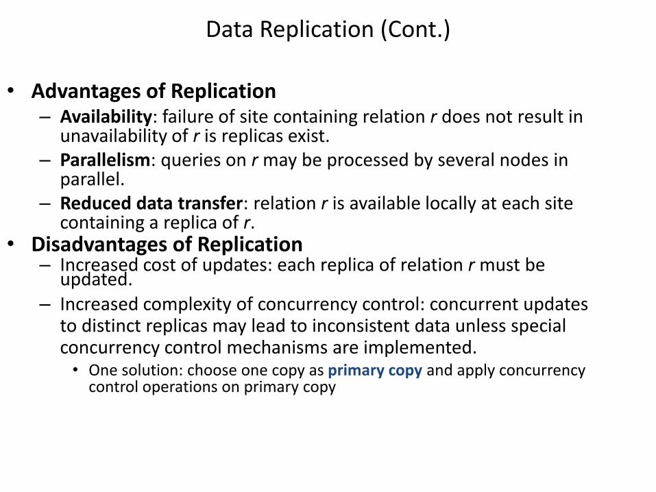
Data Replication (Cont.)

• Advantages of Replication– Availability: failure of site containing relation r does not result in

unavailability of r is replicas exist.– Parallelism: queries on r may be processed by several nodes in

parallel.– Reduced data transfer: relation r is available locally at each site

containing a replica of r.• Disadvantages of Replication

– Increased cost of updates: each replica of relation r must be updated.

– Increased complexity of concurrency control: concurrent updates to distinct replicas may lead to inconsistent data unless special concurrency control mechanisms are implemented.• One solution: choose one copy as primary copy and apply concurrency

control operations on primary copy

Data Fragmentation

• Division of relation r into fragments r1, r2, …, rn which contain sufficient information to reconstruct relation r.

• Horizontal fragmentation: each tuple of r is assigned to one or more fragments– The original relation is obtained by the union of the fragments

• Vertical fragmentation: the schema for relation r is split into several smaller schemas– All schemas must contain a common candidate key (or

superkey) to ensure lossless join property• A special attribute, the tuple-id attribute may be added to each

schema to serve as a candidate key– The original relation is obtained by the join of the fragments

• Example:– Horizontal fragmentation of an account relation, by branches– Vertical fragmentation of an employer relation, to separate the data for e.g. salaries

Advantages of Fragmentation• Horizontal:

– allows parallel processing on fragments of a relation– allows a relation to be split so that tuples are located where

they are most frequently accessed• Vertical:

– allows tuples to be split so that each part of the tuple is stored where it is most frequently accessed

– tuple-id attribute allows efficient joining of vertical fragments– allows parallel processing on a relation

• Vertical and horizontal fragmentation can be mixed– Fragments may be successively fragmented to an arbitrary

depth– An examples is to horizontally fragment an account relation by

branches, and vertically fragment it to hide balances

Data Transparency• Data transparency: Degree to which

system user may remain unaware of the details of how and where the data items are stored in a distributed system

• Transparency issues are considered in relation to:– Fragmentation transparency– Replication transparency– Location transparency

• Despite of transparency issues, data item must always be uniquely identified in the whole distributed database

Criteria for naming of data items

1.Every data item must have a system-wide unique name.

2.It should be possible to find the location of data items efficiently.

3.It should be possible to change the location of data items transparently.

4.Each site should be able to create new data items autonomously.

Centralized naming scheme - Name Server

• Structure:– name server assigns all names– each site maintains a record of local data items– sites ask name server to locate non-local data

items

• Advantages:– satisfies naming criteria 1-3

• Disadvantages:– does not satisfy naming criterion 4– name server is a potential performance

bottleneck– name server is a single point of failure

Use of Aliases• Alternative to centralized scheme: each site prefixes

its own site identifier to any name that it generates i.e., site 17.account.– Fulfills having a unique identifier, and avoids problems

associated with central control.– However, fails to achieve location transparency.

• Solution: Create a set of aliases for data items; Store the mapping of aliases to the real names at every site.

• The user can be unaware of the physical location of a data item, and is unaffected if the data item is moved from one site to another.

Distributed Transactions

• Transaction may access data at several sites.• Each site has a local transaction manager responsible for:

– Maintaining a log for recovery purposes– Participating in coordinating the concurrent execution of the

transactions executing at that site.

• Each site has a transaction coordinator, which is responsible for:– Starting the execution of transactions that originate at the site.– Distributing subtransactions at appropriate sites for execution.– Coordinating the termination of each transaction that

originates at the site, which may result in the transaction being committed at all sites or aborted at all sites.

Transaction System Architecture

System Failure Modes• Besides the failures of non-distributed systems

there are others unique to distributed systems:– Failure of a site.– Loss of messages

• Handled by network transmission control protocols such as TCP-IP

– Failure of a communication link• Handled by network protocols, by routing messages via

alternative links

– Network partition• A network is said to be partitioned when it has been split

into two or more subsystems that lack any connection between them

– Alternative routing is useless for these

• Network partitioning and site failures are generally indistinguishable.

Commit Protocols

• Commit protocols are used to ensure atomicity of global transactions, across sites– a transaction which executes at multiple sites must

either be committed at all the sites, or aborted at all the sites.

– not acceptable to have a transaction committed at one site and aborted at another – it would violate atomicity!

• The two-phase commit (2PC) protocol is widely used

• The three-phase commit (3PC) protocol is more complicated and more expensive, but avoids some drawbacks of two-phase commit protocol.

Two Phase Commit Protocol (2PC)

• Assumes fail-stop model– failed sites simply stop working, and do not cause

any other harm, such as sending incorrect messages to other sites.

• Execution of the protocol is initiated by the coordinator after the last step of the transaction has been reached.

• The protocol involves all the local sites at which the transaction executed

• Let T be a transaction initiated at site Si, and let the transaction coordinator at Si be Ci

2PC-Phase 1: Obtaining a Decision

• Coordinator asks all participants to prepare to commit transaction Ti.• Ci adds the records <prepare T> to the log and forces log to

stable storage• sends prepare T messages to all sites at which T executed

• Upon receiving message, transaction manager at remote site determines if it can commit the transaction• if not, add a record <no T> to the log and send abort T

message to Ci

• if the transaction can be committed, then:• add the record <ready T> to the log• force all records for T to stable storage• send ready T message to Ci

2PC-Phase 2: Recording the Decision

• T can be committed when Ci receives a ready Tmessage from all the participating sites: if that is not reached T must be aborted.

• Coordinator adds a decision record, <commit T> or <abort T>, to the log and forces record onto stable storage. After this, the fate of the transaction is determined (even if failure occurs afterwards)

• Coordinator sends a message to each participant informing it of the decision (commit or abort)

• Participants take appropriate action locally.

Handling of Failures in 2PC - Site Failure

When site Sk recovers, it examines its log to determine the fate oftransactions active at the time of the failure.• Log contain <commit T> record: site executes redo (T)• Log contains <abort T> record: site executes undo (T)• Log contains <ready T> record: site must consult Ci to determine

the fate of T.• If T committed, redo (T)• If T aborted, undo (T)

• The log contains no control records concerning T. Thus Sk must have failed before responding to the prepare T message from Ci

• Since, by 2PC, the failure of Sk precludes the sending of such a response C1 must abort T and Sk must execute undo (T)

Failures in 2PC - Coordinator Failure

• If coordinator fails while the commit protocol for T is executing then participating sites must decide on T’s fate:1. If an active site contains a <commit T> record in its log, then T

must be committed.2. If an active site contains an <abort T> record in its log, then T must

be aborted.3. If some active participating site does not contain a <ready T>

record in its log, then the failed coordinator Ci cannot have decided to commit T. Can therefore abort T.

4. If none of the above cases holds, then all active sites must have a <ready T> record in their logs, but no additional control records (such as <abort T> of <commit T>). In this case active sites must wait for Ci to recover, to find decision.

• Blocking problem : active sites may have to wait for failed coordinator to recover.

Handling of Failures in 2PC - Network Partition

• If the coordinator and all its participants remain in one partition, the failure has no effect on the commit protocol.

• If the coordinator and its participants belong to several partitions:– Sites that are not in the partition containing the coordinator

think the coordinator has failed, and execute the protocol to deal with failure of the coordinator.• No harm results, but sites must have to wait for decision from

coordinator.

• The coordinator and the sites are in the same partition as the coordinator think that the sites in the other partition have failed, and follow the usual commit protocol.

• Again, no harm results, but lots of failures

Concurrency Control in Distributed Databases

• Modify concurrency control schemes for use in distributed environment.

• We assume that each site participates in the execution of a commit protocol to ensure global transaction atomicity.

• We assume all replicas of any item are updated – Will see how to relax this in case of site failures

later, when studying propagation of updates with replication

1.Lociking Protocols:1.Single-Lock-Manager Approach

• System maintains a single, centralized, lock manager that resides in a single chosen site, say Si

• When a transaction needs to lock a data item, it sends a lock request to Si and lock manager determines whether the lock can be granted immediately• If yes, lock manager sends a message to the site which initiated the

request• If no, request is delayed until it can be granted, at which time a message is

sent to the initiating site• The transaction can read the data item from any one of the sites at

which a replica of the data item resides. Writes must be performed on all replicas of a data item

• Advantages of scheme:• Simple implementation• Simple deadlock handling

• Disadvantages of scheme are:• Bottleneck: lock manager site becomes a bottleneck• Vulnerability: system is vulnerable to lock manager site failure.

2.Distributed Lock Manager

• Here, functionality of locking is implemented by lock managers at each site• Lock managers control access to local data items, but special

protocols may be used for replicas

• Advantage: work is distributed and can be made robust to failures

• Disadvantage: deadlock detection is more complicated• Lock managers must cooperate for deadlock detection

• Several variants of this approacha) Primary copyb) Majority protocolc) Biased protocold) Quorum consensus

a.Primary Copy• Choose one replica of data item to be the primary copy.

– Site containing the replica is called the primary site for that data item

– Different data items can have different primary sites

• When a transaction needs to lock a data item Q, it requests a lock at the primary site of Q.– Implicitly gets lock on all replicas of the data item

• Benefit– Concurrency control for replicated data handled similarly to

unreplicated data - simple implementation.

• Drawback– If the primary site of Q fails, Q is inaccessible even though

other sites containing a replica may be accessible.

b.Majority Protocol• Local lock manager at each site administers lock and

unlock requests for data items stored at that site.• When a transaction wishes to lock an unreplicated data

item Q residing at site Si, a message is sent to Si ‘s lock manager.• If Q is locked in an incompatible mode, then the request is

delayed until it can be granted.• When the lock request can be granted, the lock manager sends

a message back to the initiator indicating that the lock request has been granted.

• In case of replicated data• If Q is replicated at n sites, then a lock request message must be

sent to more than half of the n sites in which Q is stored.• The transaction does not operate on Q until it has obtained a

lock on a majority of the replicas of Q.• When writing the data item, transaction performs writes on all

replicas.

Majority Protocol (Cont.)• Benefit

– Can be used even when some sites are unavailable• See details on how handle writes in the presence

of site failure in the book

• Drawback– Requires 2(n/2 + 1) messages for handling

lock requests, and (n/2 + 1) messages for handling unlock requests.

– Potential for deadlock even with single item:• Consider Q replicated in sites S1 to S4, and

transactions T1 and T2 requiring Q• Further consider that T1 acquired the lock in S1

and S2, and T2 at S3 and S4• None gets the majority - deadlock

c.Biased Protocol• Local lock manager at each site as in majority

protocol, however, requests for shared locks are handled differently than requests for exclusive locks.– Shared locks. When a transaction needs to lock data

item Q, it simply requests a lock on Q from the lock manager at one site containing a replica of Q.

– Exclusive locks. When transaction needs to lock data item Q, it requests a lock on Q from the lock manager at all sites containing a replica of Q.

• Advantage - imposes less overhead on read operations.

• Disadvantage - additional overhead on writes

d.Quorum Consensus Protocol

• A generalization of both majority and biased protocols• Each site is assigned a weight.

• Let S be the total of all site weights

• Choose two values read quorum Qr and write quorum Qw

• Such that Qr + Qw > S and 2 * Qw > S• Quorums can be chosen (and S computed) separately for each

item

• Each read must lock enough replicas that the sum of the site weights is >= Qr

• Each write must lock enough replicas that the sum of the site weights is >= Qw

• For now we assume all replicas are written• Extensions to allow some sites to be unavailable described later

2.Timestamping for global transactions

• Timestamp based concurrency-control protocols can be used in distributed systems

• Each transaction must be given a unique timestamp

• Main problem: how to generate a timestamp in a distributed fashion– Each site generates a unique local timestamp using

either a logical counter or the local clock.

– Global unique timestamp is obtained by concatenating the unique local timestamp with the unique identifier (that must be at the end!).

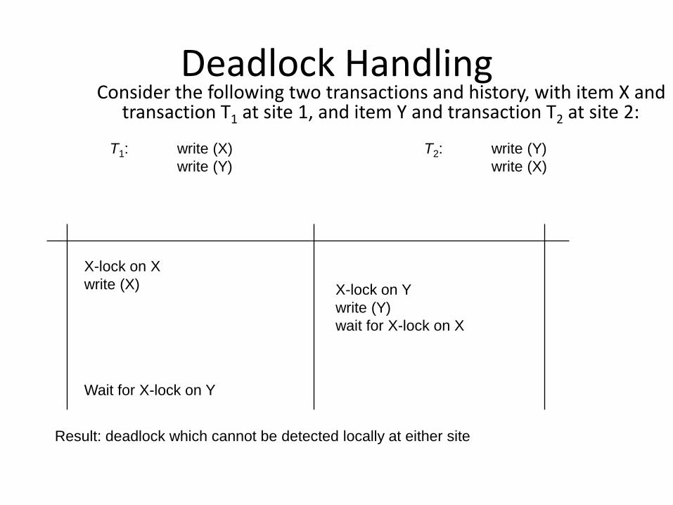
Deadlock HandlingConsider the following two transactions and history, with item X and

transaction T1 at site 1, and item Y and transaction T2 at site 2:

T1: write (X)

write (Y)

T2: write (Y)

write (X)

X-lock on X

write (X) X-lock on Y

write (Y)

wait for X-lock on X

Wait for X-lock on Y

Result: deadlock which cannot be detected locally at either site

Centralized approach to deadlock detection• A global wait-for graph is constructed and maintained

in a single site; the deadlock-detection coordinator– Real graph: Real, but unknown, state of the system.– Constructed graph:Approximation generated by the

controller during the execution of its algorithm .

• the global wait-for graph can be constructed when:– a new edge is inserted in or removed from one of the

local wait-for graphs.– a number of changes have occurred in a local wait-for

graph.– the coordinator needs to invoke cycle-detection.

• If the coordinator finds a cycle, it selects a victim and notifies all sites. The sites roll back the victim transaction.

Local and Global Wait-For Graphs

Local

Global

Example Wait-For Graph for False CyclesInitial state:

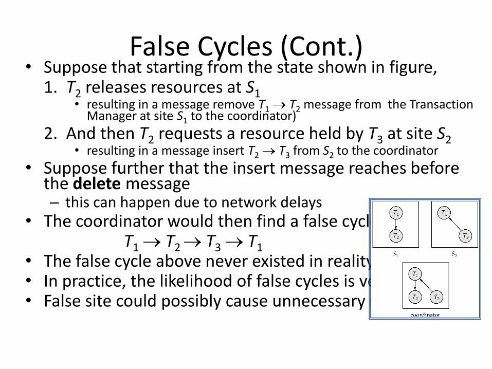
False Cycles (Cont.)• Suppose that starting from the state shown in figure,

1. T2 releases resources at S1• resulting in a message remove T1 T2 message from the Transaction

Manager at site S1 to the coordinator)

2. And then T2 requests a resource held by T3 at site S2• resulting in a message insert T2 T3 from S2 to the coordinator

• Suppose further that the insert message reaches before the delete message – this can happen due to network delays

• The coordinator would then find a false cycle T1 T2 T3 T1

• The false cycle above never existed in reality.• In practice, the likelihood of false cycles is very low!• False site could possibly cause unnecessary rollbacks.

Availability

• High availability: time for which system is not fully usable should be extremely low (e.g. 99.99% availability)

• Robustness: ability of system to function spite of failures of components

• Failures are more likely in large distributed systems• To be robust, a distributed system must

– Detect failures– Reconfigure the system so computation may continue– Recovery/reintegration when a site or link is repaired

• Failure detection: distinguishing link failure from site failure is hard– (partial) solution: have multiple links, multiple link failure is

likely a site failure

Reconfiguration

• Reconfiguration:– Abort all transactions that were active at a failed site

• Making them wait could interfere with other transactions since they may hold locks on other sites

• However, in case only some replicas of a data item failed, it may be possible to continue transactions that had accessed data at a failed site

– If replicated data items were at failed site, update system catalog to remove them from the list of replicas. • This should be reversed when failed site recovers, but additional care

needs to be taken to bring values up to date

– If a failed site was a central server for some subsystem, an election must be held to determine the new server• E.g. name server, concurrency coordinator, global deadlock detector

Reconfiguration (Cont.)• Since network partition may not be

distinguishable from site failure, the following situations must be avoided– Two ore more central servers elected in distinct

partitions– More than one partition updates a replicated

data item

• Updates must be able to continue even if some sites are down

• Solution: majority based approach– Alternative of “read one write all available” is

tantalizing but causes problems

1.Majority-Based Approach

• The majority protocol for distributed concurrency control can be modified to work even if some sites are unavailable– Each replica of each item has a version number which

is updated when the replica is updated– A lock request is sent to at least ½ the sites at which

item replicas are stored and operation continues only when a lock is obtained on a majority of the sites

– Read operations look at all replicas locked, and read the value from the replica with largest version number• May write this value and version number back to replicas

with lower version numbers (no need to obtain locks on all replicas for this task)

Majority-Based Approach• Majority protocol (Cont.)

– Write operations• Find highest version number like reads, and set new version number to

old highest version + 1• Writes are then performed on all locked replicas and version number

on these replicas is set to new version number

– Failures (network and site) cause no problems as long as • Sites at commit contain a majority of replicas of any updated data

items• During reads a majority of replicas are available to find version

numbers• Subject to above, 2 phase commit can be used to update replicas

– Note: reads are guaranteed to see latest version of data item– Reintegration is trivial: nothing needs to be done

• Quorum consensus algorithm can be similarly extended

2.Read One Write All (Available)

• Biased protocol is a special case of quorum consensus– Allows reads to read any one replica but updates require all replicas to

be available at commit time (called read one write all)

• Read one write all available (ignoring failed sites) is attractive, but incorrect– If failed link may come back up, without a disconnected site ever being

aware that it was disconnected– The site then has old values, and a read from that site would return an

incorrect value– If site was aware of failure reintegration could have been performed,

but no way to guarantee this– With network partitioning, sites in each partition may update same

item concurrently• believing sites in other partitions have all failed

Coordinator Selection• Backup coordinators

– site which maintains enough information locally to assume the role of coordinator if the actual coordinator fails

– executes the same algorithms and maintains the same internal state information as the actual coordinator fails executes state information as the actual coordinator

– allows fast recovery from coordinator failure but involves overhead during normal processing.

• Election algorithms– Used to elect a new coordinator in case of failures – Example: Bully Algorithm - applicable to systems where every

site can send a message to every other site.• To simplify assume sites are identified by numbers, and the

coordinator should always be the one with highest number

Bully Algorithm• If site Si sends a request that is not answered by the coordinator within

a time interval T, assume that the coordinator has failed Si tries to elect itself as the new coordinator.

• Si sends an election message to every site with a higher identification number, and then waits for any of these processes to answer within T.

• If no response within T, assume that all sites with number greater than i have failed, Si elects itself the new coordinator.

• If answer is received Si begins time interval T’, waiting to receive a message that a site with a higher identification number has been elected.

• If no message is sent within T’, assume the site with a higher number has failed; Si restarts the algorithm.

• After a failed site recovers, it immediately begins execution of the same algorithm.

• If there are no active sites with higher numbers, the recovered site forces all processes with lower numbers to let it become the coordinator site, even if there is a currently active coordinator with a lower number.

Distributed Query Processing

• For centralized systems, the primary criterionfor measuring the cost of a particular strategy is the number of disk accesses.

• In a distributed system, other issues must be taken into account:

– The cost of a data transmission over the network.

– The potential gain in performance from having several sites process parts of the query in parallel.

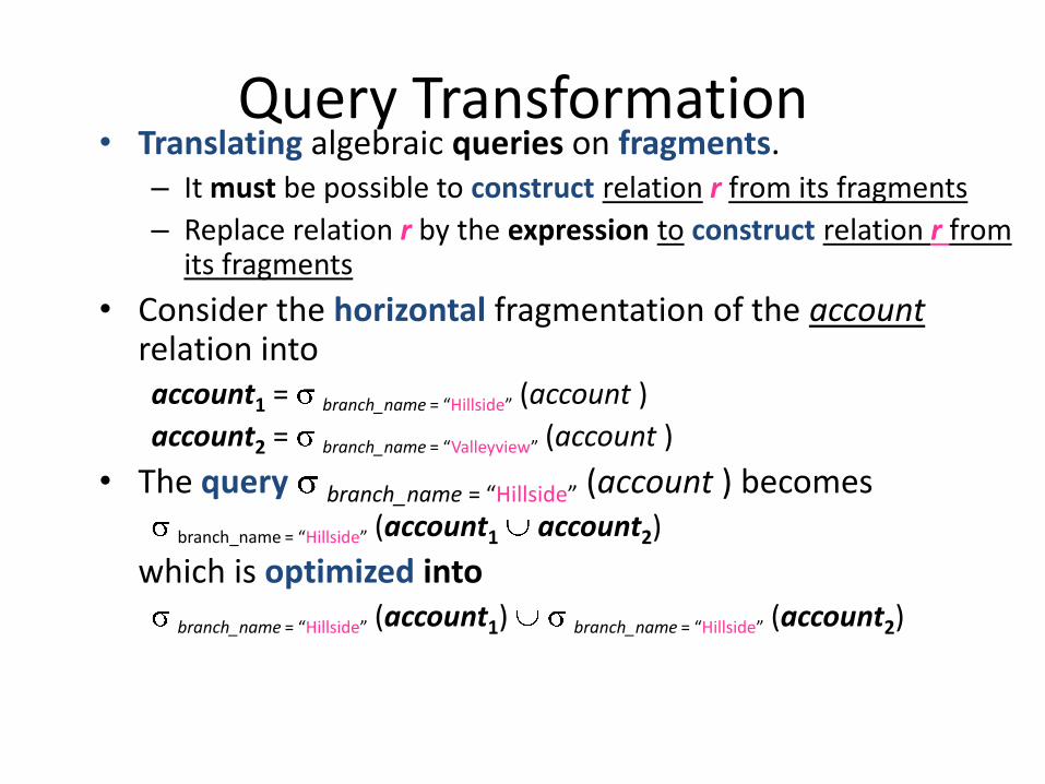
Query Transformation• Translating algebraic queries on fragments.

– It must be possible to construct relation r from its fragments

– Replace relation r by the expression to construct relation r from its fragments

• Consider the horizontal fragmentation of the accountrelation intoaccount1 = branch_name = “Hillside” (account )

account2 = branch_name = “Valleyview” (account )

• The query branch_name = “Hillside” (account ) becomes

branch_name = “Hillside” (account1 account2)

which is optimized into

branch_name = “Hillside” (account1) branch_name = “Hillside” (account2)

Example Query (Cont.)

• Since account1 has only tuples pertaining to the Hillside branch, we can eliminate the selection operation.

• Apply the definition of account2 to obtainbranch_name = “Hillside” ( branch_name = “Valleyview” (account )

• This expression is the empty set regardless of the contents of the account relation.

• Final strategy is for the Hillside site to return account1as the result of the query.

Simple Join Processing• Consider the following relational algebra

expression in which the three relations are neither replicated nor fragmentedaccount depositor branch

• account is stored at site S1

• depositor at S2

• branch at S3

• For a query issued at site SI, the system needs to produce the result at site SI

Possible Query Processing Strategies

• Ship copies of all three relations to site SI and choose a strategy for processing the entire locally at site SI.

• Ship a copy of the account relation to site S2 and compute temp1 = account depositor at S2. Shiptemp1 from S2 to S3, and compute temp2 = temp1branch at S3. Ship the result temp2 to SI.

• Devise similar strategies, exchanging the roles S1, S2, S3

• Must consider following factors:– amount of data being shipped– cost of transmitting a data block between sites– relative processing speed at each site

Semijoin Strategy

• Let r1 be a relation with schema R1 stores at site S1

Let r2 be a relation with schema R2 stores at site S2

• Evaluate the expression r1 r2 and obtain the result at S1.– 1. Compute temp1 R1 R2 (r1) at S1.– 2. Ship temp1 from S1 to S2.

– 3. Compute temp2 r2 temp1 at S2

– 4. Ship temp2 from S2 to S1.

– 5. Compute r1 temp2 at S1. This is the same as r1 r2.

Formal Definition

• The semijoin of r1 with r2, is denoted by:r1 r2

• it is defined by:• R1 (r1 r2)• Thus, r1 r2 selects those tuples of r1 that

contributed to r1 r2.• In step 3 above, temp2=r2 r1.• For joins of several relations, the above strategy

can be extended to a series of semijoin steps.

Heterogeneous Distributed Databases

• Many database applications require data from a variety of preexisting databases located in a heterogeneouscollection of hardware and software platforms

• Data models may differ (hierarchical, relational , etc.)• Transaction commit protocols may be incompatible• Concurrency control may be based on different

techniques (locking, timestamping, etc.)• System-level details almost certainly are totally

incompatible.• A multidatabase system is a software layer on top of

existing database systems, which is designed to manipulate information in heterogeneous databases– Creates an illusion of logical database integration without

any physical database integration

Advantages

• Preservation of investment in existing– hardware– system software– Applications

• Local autonomy and administrative control • Allows use of special-purpose DBMSs• Step towards a unified homogeneous DBMS

– Full integration into a homogeneous DBMS faces:• Technical difficulties and cost of conversion• Organizational/political difficulties

– Organizations do not want to give up control on their data– Local databases wish to retain a great deal of autonomy

Directory Systems• Typical kinds of directory information

– Employee information such as name, id, email, phone, office addr, ..– Even personal information to be accessed from multiple places

• e.g. Web browser bookmarks

• White pages– Entries organized by name or identifier

• Meant for forward lookup to find more about an entry

• Yellow pages– Entries organized by properties– For reverse lookup to find entries matching specific requirements

• When directories are to be accessed across an organization– Alternative 1: Web interface. Not great for programs– Alternative 2: Specialized directory access protocols

• Coupled with specialized user interfaces

Directory Access Protocols

• Most commonly used directory access protocol:– LDAP (Lightweight Directory Access Protocol)– Simplified from earlier X.500 protocol

• Question: Why not use database protocols like ODBC/JDBC?

• Answer: – Simplified protocols for a limited type of data access, evolved

parallel to ODBC/JDBC– Provide a nice hierarchical naming mechanism similar to file

system directories• Data can be partitioned amongst multiple servers for different parts

of the hierarchy, yet give a single view to user– E.g. different servers for Bell Labs Murray Hill and Bell Labs Bangalore

– Directories may use databases as storage mechanism