data warehousing & data mining - tu braunschweig · data warehousing & data mining ... –...

Data Warehousing & Data Mining& Data MiningWolf-Tilo BalkeSilviu HomoceanuInstitut für InformationssystemeTechnische Universität Braunschweighttp://www.ifis.cs.tu-bs.de

3.1 Basics of data modeling

3.2 Data models in DW

� 3.2.1 Conceptual Modeling

� 3.2.2 Logical Modeling

3.3 Best Practices

3. DW Modeling

3.3 Best Practices

Data Warehousing & OLAP – Wolf-Tilo Balke – Institut für Informationssysteme – TU Braunschweig 2

• Data Modeling / DB Design

– Is the process of creating a data model by analyzing the requirements needed to support the business processes of an organization

• It is sometimes called database

3.1 Basics of Data Modeling

• It is sometimes called database

modeling/design because a data

model is eventually implemented

in a database


• Data models– Provide the definition and format of data

– Graphical representations of the data within a specific area of interest

• Enterprise Data Model: represents the integrated data requirements of a complete business organization

3.1 Basics of Data Modeling

requirements of a complete business organization

• Subject Area Data Model: Represents the data requirements of a single business area or application

– Used to clearly convey the meaning of data, the relationships amongst data, the attributes of the data and the precise definitions of data

– The standard and accepted way of analyzing data, and a prerequisite for designing and implementing a database


3.1 Phases of Data ModelingRequirement

Analysis

Conceptual

Design

Functional

Analysis

Data requirements

Conceptual schema


Physical Design

Application

Program Design

Transaction

Implementation

Logical Design

Logical schema

DBMS Independent

DBMS Dependent

Application

• Conceptual Design– Transforms data requirements to conceptual model– Conceptual model describes data entities, relationships, constraints,

etc. on high-level• Does not contain any implementation details• Independent of used software and hardware

• Logical Design

3.1 Phases of Data Modeling

• Logical Design– Maps the conceptual data model to the logical data model used by

the DBMS• e.g. relational model, dimensional model, …• Technology independent conceptual model is adapted to the used DBMS

software

• Physical Design– Creates internal structures needed to efficiently store/manage data

• Table spaces, indexes, access paths, …• Depends on used hardware and DBMS software


• Going from one phase to the next:• The phase must be complete

– The result serves as input for the next phase

• Often automatic transition is possible with additional designer feedback

3.1 Phases of Data Modeling

designer feedback


Conceptual

Design Logical

DesignPhysical

DesignER-diagram,

UML, … Tables,

Columns, …Tablespaces,

Indexes, …

• Highest conceptual grouping of ideas

– Data tends to naturally cluster with data from the same or similar categories relevant to the organization

• The major relationships between subjects have

3.1 Conceptual Model

• The major relationships between subjects have been defined

– Least amount of detail


• Conceptual design

– See RDB1 course

– Entity-Relationship (ER) Modeling

• Entities - “things” in the real world

E.g. Car, Account, Product


Conceptual

Design

ER-diagram,

UML, …

Car Account Product– E.g. Car, Account, Product

• Attributes – property of an entity, entity type, or relationship type

– E.g. color of a car, balance of an account, price of a product

• Relationships – between entities there can be relationships, which also can have attributes

– E.g. Person owns Car


Car Account Product

Car ColorColor

CarownsPerson


Student Professor

registration

number

registration

number

name

name department

id

attends teaches

instantiates

time

day of

week

day of

weekroom

semester

Lecture

instance

1

N N 1 N

1


title credits

id Lecture

Course of

Study

enrolls

name

part of

prereq.

curriculum

semester

curriculum

semester

N

N

N

N

N

N

• Conceptual design in usually done using the Unified Modeling Language (UML)

– Class Diagram, Component Diagram, Object Diagram, Package Diagram…

– For Data Modeling only Class Diagrams are used


Conceptual

Design

ER-diagram,

UML, …

– For Data Modeling only Class Diagrams are used

• Entity type becomes class

• Relationships become associations

• There are special types of associations like: aggregation, composition, or generalization


CLASS NAME

attribute 1 : domain

attribute n : domain

operation 1

operation m

…

…

• Logical design arranges data into a logical structure

– Which can be mapped into the storage objects supported by DBMS

• In the case of RDB, the storage objects are tables which

3.1 Logical Model

Logical

Design

Tables,

Columns,

…

• In the case of RDB, the storage objects are tables which store data in rows and columns


Relation

Attribute

Tuple

• Physical design specifies the physical configuration of the database on the storage media

– detailed specification of:data elements, data types,

3.1 Physical Model

Physical

Design

Tablespaces

Indexes

data elements, data types,

indexing options, and

other parameters

residing in the DBMS

data dictionary


• Managing Complex Data Relationships

– Helps keep track of the complex environment that is a DW

• Many complex relationships exist, with the ability to change over time

3.2 Data Model in DW

over time

– Transformations and integration from various systems of record need to be worked out and maintained

– Provides the means of supplying users with a roadmap through the data and relationships


• Modeling business queries

– Goal

• Define the purpose, and decide on the subject(s) for the data warehouse

• Identify questions of interest

3.2.1 Conceptual Model

Time

• Identify questions of interest

– Subject

• Who bought the products?

(customers and their structure)

• Who sold the product? (sales organization)

• What was sold? (product structure)

• When was it sold? (time structure)


CustomersEmployees

Products

Business

Model

• For Conceptual design in DW conventional techniques like E/R or UML are not appropriate

– Lack of necessary semantics for modeling the multidimensional data model

– E/R are constituted to


– E/R are constituted to

• Remove redundancy in the data model

• Facilitate retrieval of individual records

– Therefore optimize OLTP

– In the case of DW, however redundancy and Materialized Views help speed up Analytical queries


– Design models for DW

• Multidimensional Entity Relationship (ME/R) Model

• Multidimensional UML (mUML)

• Dimensional Fact Model (DFM)

• Other methods like e.g.,


• Other methods like e.g., the Totok approach


• ME/R Model

– Its purpose is to create an intuitive representationof the multidimensional data that is optimized for high-performance access

– It represents a specialization and evolution of the E/R

3.2.1 Multidim. E/R Model

– It represents a specialization and evolution of the E/R to allow specification of multidimensional semantics


• ME/R notation was influenced by the following considerations– Specialization of the E/R model

• All new elements of the ME/R have to be specializations of the E/R elements

• In this way the flexibility and power of expression of the E/R


• In this way the flexibility and power of expression of the E/R models are not reduced

– Minimal expansion of the E/R model• Easy to understand/learn/use: the number of additional elements should be small

– Representation of the multidimensional semantics• Although being minimal, it should be powerful enough to be able

to represent multidimensional semantics


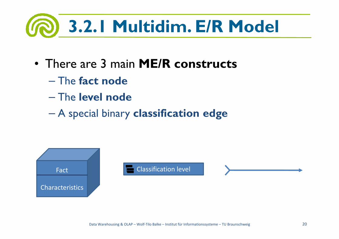
• There are 3 main ME/R constructs

– The fact node

– The level node

– A special binary classification edge


A special binary classification edge


Fact

Characteristics

Classification level

• Lets consider a store scenario designed in E/R

– Entities bear little semantics

– E/R doesn’t support classification levels


Package


Article Store

Product Product

group

Package CityDistrict NameDate

Article Nr

is sold

Is

in

Is

packed

in

Belongs Belongs

to

Is in

1

1

nn

n

m

• ME/R notation:


ArticleProd. GroupProd. FamilyProd. Categ


Sales

Characteristics

StoreCityDistrictRegionCountry

Week

DayMonthQuarterYear

• ME/R notation:

– Sales was elected as fact node

– The dimensions are product, geographical area and time


– The dimensions are represented

through the so called Basic

Classification Level

– Alternative paths in the classification level are also possible


Week

DayMonth

Sales

Characteristics

Store

Article

Day

• UML is a general purpose modeling language

• It can be tailored to specific domains through the use of the following mechanisms

– Stereotypes: building new elements

3.2.1 Unified Modeling Language

– Stereotypes: building new elements

– Tagged values: new properties

– Constraints: new semantics


• Stereotype

– Grants a special semantics to an UML construction without modifying it

– There are 4 possible representations of the stereotype in UML

3.2.1 mUML

stereotype in UML


Icon Decoration Label None

Fact 1

Fact 2<<Fact>>

Fact 3Fact 4

• Tagged value

– Define properties by using a pair of tag and data value

• Tag = Value

• E.g. formula=“UnitsSold*UnitPrice”

3.2.1 mUML

• E.g. formula=“UnitsSold*UnitPrice”


<<Fact-Class>>

Sales

UnitsSold: Sales

UnitPrice: Price

/VolumeSold: Price

{formula=“UnitsSold*UnitPrice”

, parameter=“UnitsSold,

UnitPrice”}

3.2.1 mUML

<<Dimensional-Class>>

Week


Month


Quarter


Year


City


Region


Land

<<Roll-up>>

Distributor Country

<<Roll-up>>

Country

<<Roll-up>>

Region

<<Roll-up>>

Year

<<Roll-up>>

Quarter

<<Shared -Roll-up>>

Year

1..2


<<Fact-Class>>

Sold products

<<Fact-Class>>

Sales


Day

1..*

<<Dimension>>

Time


Store


Prod. Categ


Prod. Group


Product

<<Dimension>>

Geography

<<Dimension>>

Product

<<Roll-up>>

Product categ

<<Roll-up>>

Product Group

<<Roll-up>>

City<<Roll-up>>

Week

<<Roll-up>>

Month

• DFM consists of a set of fact schemes

• Components of a fact scheme are– Facts: a fact is a focus of interest for decision-making,

e.g., sales, shipments..

– Measures: attributes that describe facts from different

3.2.1 Dimensional Fact Model

– Measures: attributes that describe facts from different points of view, e.g. , each sale is measured by its revenue

– Dimensions: discrete attributes which determine the granularity adopted to represent facts, e.g. , product, store, date

– Hierarchies: are made up of dimension attributes• Determine how facts may be aggregated and selected, e.g. ,

day – month – quarter - year


3.2.1 Dimensional Fact Model


• Goal

– Define our functional requirements

– Confirm the subject areas

– Figure out what the time dimension means

3.2.2 Logical Model

Figure out what the time dimension means

– Identify the granularity (how deep can we go) for our subject(s)

– Create ‘real’ facts and dimensions from the subjects that we have identified


• Logical structure of the multidimensional model

– Cubes: Sales, Purchase, Price, Inventory

– Dimensions: Product, Time, Geography, Client

3.2.2 Logical Model


Purchase

Amount



Week

DayMonthQuarterYear

Price

Unit Price

Inventory

Stock

Sales

TurnoverClient

• Analysis purpose chosen entities, within the data model

– One dimension can be used to define

more than one cube

3.2.2 Dimensions

more than one cube

– They can be also hierarchically organized


Purchase

AmountArticleProd. GroupProd. FamilyProd. Categ

Price

Unit Price

Sales

Turnover

• Hierarchies

– The dependencies between the classification levels are described by the classification schema (Roll-upconnections)

• Roll-up connections can be described by functional

3.2.2 Dimensions

• Roll-up connections can be described by functional dependencies

• An attribute B is functionally dependent on an attribute A, denoted A ⟶ B, if for all a ∈ dom(A) there exists exactly one b ∈ dom(B) corresponding to it


Week

DayMonthQuarterYear

• Classification schemas

– The classification schema of a dimension D is a semi-ordered set of classification levels ({D.K0, …, D.Kk}, ⟶ )

– With a smallest element D.K ,

3.2.2 Dimensions

⟶

– With a smallest element D.K0, i.e. there is no classification level with smaller granularity


• A fully-ordered set of classification levels is called a Path

– If we consider the classification schema of the time dimension, then we have the following paths

• T.Day T.Week

3.2.2 Dimensions

• T.Day T.Week

• T.Day T.Month T.Quarter T.Year

– Here T.Day is the smallest element


DayMonthQuarterYear

Week

• Classification hierarchies

– Let D.K0 ⟶ …⟶ D.Kk be a path in the classification schema of dimension D

– A classification hierarchy concerning these path is a balanced tree which

3.2.2 Dimensions

a balanced tree which

• Has as nodes dom(D.K0) U … U dom(D.Kk) U {ALL}

• And its edges respect the functional dependencies


• Example: classification hierarchy from the path product dimension

3.2.2 Dimensions


ALL


Electronics

Video Audio

Video

recorder

Video

recorderCamcorder

TR-34 TS-56

…

…

TV

…

Clothes

…

Article

Prod. Group

Prod. Family

Category

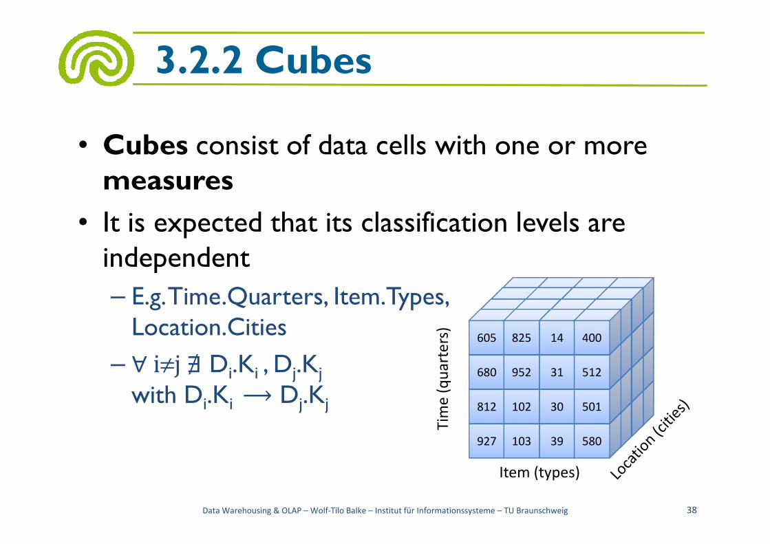
• Cubes consist of data cells with one or more measures

• It is expected that its classification levels are independent

3.2.2 Cubes

independent

– E.g. Time.Quarters, Item.Types, Location.Cities

– ∀ i≠j ∄ Di.Ki , Dj.Kj

with Di.Ki ⟶ Dj.Kj


927 103

812 102

39 580

30 501

680 952

818605 825

31 512

14 400

Item (types)

Tim

e (

qu

art

ers

)

• Cube schema

– A cube schema, S(G,M), consists of a Granularity G and a set M=(M1, …, Mm) representing the measure

• The measure is usually represented by numerical attributes, here the number of sells

3.2.2 Cubes

here the number of sells

• The granularity is here represented by quarters, types and cities


927 103

812 102

39 580

30 501

680 952

818605 825

31 512

14 400

Item (types)

Tim

e (

qu

art

ers

)

• A Cube (CCCC) is a set of cube cells, C ⊆ dom(G) x

dom(M)

– The coordinates of a cell are the classification nodes from dom(G) corresponding to the cell

• Sales ((Article, Day, Store, Client), (Turnover))

3.2.2 Cubes

dom(G)

• Sales ((Article, Day, Store, Client), (Turnover))

• Purchase ((Article, Day, Store),(Amount))

• Price ((Article, Day),(Unit Price))

• Inventory (…)


3.2.2 Cubes

818605 825 14 400

818… … … …

Supplier = s1 Supplier = s2 Supplier = s3

818… … … …

BerlinMünchen

ParisBraunschweig

Q1

• 4 dimensions (supplier, city, quarter, product)


927 103

812 102

39 580

30 501

680 952

605 825

31 512

14 400

… …

… …

… …

… …

… …

… …

… …

… …

… …

… …

… …

… …

… …

… …

… …

… …Q1

Q2

Q3

Q4

Co

mp

ute

r

Vid

eo

Au

dio

Tele

ph

on

es

Co

mp

ute

r

Vid

eo

Au

dio

Tele

ph

on

es

Co

mp

ute

r

Vid

eo

Au

dio

Tele

ph

on

es

– We can now imagine n-dimensional cubes

• n-D cube is called a base cuboid

• The top most cuboid, the 0-D, which holds the highest level of summarization is called apex cuboid

• The full data cube is formed by the lattice of cuboids

3.2.2 Cubes

• The full data cube is formed by the lattice of cuboids


• But things can get complicated pretty fast

3.2.2 Cubes

all

time supplier

0-D(apex) cuboid

1-D cuboids

item location


time,item time,location

time,supplier

item,location

item,supplier

location,supplier

time,item,location

time,item,supplier

time,location,supplier

item,location,supplier

time, item, location, supplier

2-D cuboids

3-D cuboids

4-D(base) cuboid

• Basic operations of the multidimensional model

– Selection

– Projection

– Cube join

3.2.2 Basic Operations

Cube join

– Sum

– Aggregation


• Multidimensional Selection

– The selection on a cube C((D1.K1,…, Dg.Kg),

(M1, …, Mm)) through a predicate P, is defined as σP(C) = {z Є C:P(z)}, if all variables in P are either:

• Classification levels K , which functionally depend on a K D .K ⟶ K


(M , …, M )) P

σP(C) = {z Є C:P(z)}, P

• Classification levels K , which functionally depend on a classification level in the granularity of K, i.e. Di.Ki ⟶ K

• Measures from (M1, …, Mm)

– E.g. σP.Prod_group=“Video”(Sales)


• Multidimensional projection

– The projection of a function of a measure F(M) of cube C is defined as

/F(M)(C) = { (g,F(m)) ∈ dom(G) x dom(F(M)): (g,m) ∈ C}

– E.g. , price projection /turnover, sold_items(Sales)


C

/F(M)(C) = { (g,F(m)) dom(G) x dom(F(M)): (g,m) C}

– E.g. , price projection /turnover, sold_items(Sales)


Sales

Turnover

Sold_items

• Cube join

– Join operations between cubes is usual

• E.g. if turnover would not be provided, it could be calculated with the help of the unit price from the price cube

– Joining cubes

C (G , M ) C (G , M )


– Joining cubes

• 2 cubes C1(G1, M1) and C2(G2, M2) can only be joined, if they have the same granularity (G1= G2 = G)

• C1⋈C2= C(G, M1∪ M2)


Price

Unit Price

Sales

Units_Sold

– When the granularities are different, but we still need to join the cubes, aggregation has to be performed

• E.g. , Sales ⋈ Inventory

• We need to aggregate Sales((Day, Article, Store, Client)) to Sales((Month, Article, Store, Client))


Sales((Month, Article, Store, Client))




Week

DayMonthQuarterYear

Inventory

Stock

Sales

Turnover

Client

• Aggregation

– Most important operation of cubes

– OLAP operations are based on aggregation

– Aggregation functions


Aggregation functions

• Build a single values from set of value, e.g. in SQL: SUM, AVG, Count, Min, Max

• Example: SUM(P.Product_group, G.City, T.Month)(Sales)

• Sample aggregation with smaller granularity is SUM(P.Product , G.City, T.Month)(Sales)


• Comparing granularities

– A granularity G={D1.K1, …, Dg.Kg} has a smaller or same granularity as G’={D1’.K1’, …, Dh’.Kh’},

if and only if for each Dj’.Kj’∈ G’ ∃ Di.Ki ∈ G where D .K ⟶ D ’.K ’


G’={D ’.K ’, …, D ’.K ’},

Dj’.Kj’ G’ ∃ Di.Ki G

Di.Ki ⟶ Dj’.Kj’


• Classification schema, cube schema, classification hierarchy are all designed in the building phase and considered as fix– Practice has proven otherwise

– DW grow old, too

3.2.2 Change support

– DW grow old, too

– Changes are strongly connected to the time factor

– This lead to the time validity of these concepts

• Reasons for schema modification– New requirements

– Modification of the data source


• E.g. Saturn sells a lot of electronics

– Lets consider mobile phones

• They built their DW on 01.03.2003

• A classification hierarchy of their data until 01.07.2007 could look

3.2.2 Classification Hierarchy

data until 01.07.2007 could look like this:


Mobile Phone

GSM 3G

Nokia 3600 O2 XDABlackBerry

Bold

• After 01.07.2007 3G becomes hip and affordable and many phone makers start migrating towards 3G capable phones

– Lets say O2 makes its XDA 3G capable



Mobile Phone

GSM 3G


Bold

• After 01.04.2009 phone makers already develop 4G capable phones


Mobile Phone


GSM 3G


Bold

4G

Best phone

ever

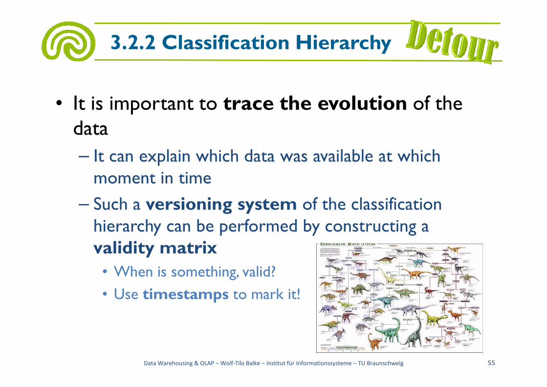
• It is important to trace the evolution of the data

– It can explain which data was available at which moment in time

– Such a versioning system of the classification


– Such a versioning system of the classification hierarchy can be performed by constructing a validity matrix

• When is something, valid?

• Use timestamps to mark it!


• Annotated Change data


Mobile Phone

[01.03.2003, ∞)[01.04.2005, ∞)

[01.04.2009, ∞)

Relational Database Systems 1 – Wolf-Tilo Balke – Institut für Informationssysteme – TU Braunschweig 56

GSM 3G


Bold

4G

Best phone

ever

[01.03.2003, ∞)[01.04.2005, ∞)

[01.04.2009, ∞)

[01.04.2009, ∞)[01.04.2005, ∞)

[01.03.2006, ∞)

[01.07.2007, ∞)

[01.03.2003, 01.07.2007)

• The tree can be stored as dimension metadata

– The storage form is a validity matrix

• Rows are parent nodes

• Columns are child nodes


GSM 3G 4G Nokia 3600 O2 XDA Berry Bold Best phone


Mobile

phone

[01.03.2003, ∞) [01.04.2005, ∞) [01.04.2009, ∞)

GSM [01.04.2005, ∞) [01.03.2003,

01.07.2007)

3G [01.07.2007, ∞) [01.03.2006, ∞)

4G [01.04.2009

, ∞)

Nokia 3600

O2 XDA

Berry Bold

Best phone

• Deleting a node in a classification hierarchy

– Should be performed only in exceptional cases

• It can lead to information loss

• How do we solve it?

– Soon GSM phones will not be produced anymore


– Soon GSM phones will not be produced anymore

• We might want to query data since when GSM was sold

• Just mark the end validity date of the GSM branch in the validity matrix


• Query classification

– Having the validity information we can support queries like as is versus as is

• Regards all the data as if the only valid classification hierarchy is the present one


hierarchy is the present one

• In the case of O2 XDA, it will be considered as it has always been a 3G phone


Mobile Phone

GSM 3G

Nokia 3600 O2 XDA BlackBerry Bold

4G

Best phone

ever

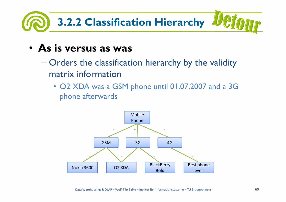
• As is versus as was

– Orders the classification hierarchy by the validity matrix information

• O2 XDA was a GSM phone until 01.07.2007 and a 3G phone afterwards


phone afterwards


Mobile

Phone

GSM 3G


Bold

BlackBerry

Bold

4G

Best phone

ever

Best phone

ever

…

… …

… …

……

• As was versus as was

– Past time hierarchies can bereproduced

– E.g., query data with anolder classification


Mobile Phone

GSM 3G

…

……

…

…older classificationhierarchy

• Like versus like

– Only data whose classification hierarchy remained unmodified, is evaluated

– E.g. the Nokia 3600 and the Black Berry



Bold

• Improper modification of a schema (deleting a dimension level) can lead to– Data loss

– Inconsistencies• Data is incorrectly aggregated or adapted

3.2.2 Dimension schema

• Proper schema modification is complex but– It brings flexibility for the end user

• The possibility to ask “As Is vs. As Was” queries and so on

• Alternatives– Schema evolution

– Schema versioning


• Schema evolution

– Modifications can be performed without data loss

– It involves schema modification and data adaptation to the new schema

– This data adaptation process is called Instance

3.2.2 Schema modification

– This data adaptation process is called Instance adaptation


Purchase

Amount


Price

Unit Price

Sales

Turnover

• Schema evolution

– Advantage

• Faster to execute queries in DW with many schema modifications

– Disadvantages


– Disadvantages

• It limits the end user flexibility to query based on the past schemas

• Only actual schema based queries are supported


• Schema versioning

– Also no data loss

– All the data corresponding to all the schemas are always available

– After a schema modification the data is held in their belonging schema


belonging schema

• Old data - old schema

• New data - new schema


Purchase

Amount


Price

Unit Price

Sales

Turnover

Purchase

Amount

ArticleProd. GroupProd. CategSales

Turnover

….

• Schema versioning

– Advantages

• Allows higher flexibility, e.g., “As Is vs. As Was”, etc. queries

– Disadvantages

• Adaptation of the data to the queried schema is done on the spot


the spot

• This results in longer query run time


• Kimball’s 9 step methodology to model a DW

1. Choosing the process

1. Decide on which data mart should be able to deliver on time, within budget, and to answer important business

3.3 Best Practices

time, within budget, and to answer important business questions

2. Choosing the grain

1. Decide on what a fact table record represents


3. Identifying and conforming the dimensions

1. Makes the data mart understandable and easy to use

2. Dimensions are identified in sufficient detail to describe things at the correct grain

3. Conformed dimensions must be the exact same

3.3 Best Practices

3. Conformed dimensions must be the exact same dimension or a mathematical subset of a dimension

4. Dimension models containing multiple fact tables that share one or more conformed dimension tables is called fact constellation


4. Choosing the facts

1. The grain of the fact table determines which facts can be used in the data mart

2. Facts should be numeric and additive

3. Facts can be added to a fact table at any time if they are

3.3 Best Practices

3. Facts can be added to a fact table at any time if they are consistent with the grain of the table


5. Storing pre-calculations in the fact table

1. Re-examine the facts to determine whether pre-calculations can be used

2. Pre-calculations derive other valuable information

6. Rounding out the dimension tables

3.3 Best Practices

6. Rounding out the dimension tables

1. Add text descriptions to dimension tables wherever possible


7. Choosing the duration of the database

1. How far back in time the fact table goes

2. Long duration cause problems:

3. Hard to read/interpret old files/tapes

4. Old versions of the important dimensions must be used

3.3 Best Practices

4. Old versions of the important dimensions must be used rather than the most current ones


8. Tracking slowly changing dimensions

1. A generalized key to important dimensions can distinguish multiple snapshots of entities over time

2. Types of slowly changing dimensions:

1. Type 1 - changed dimension attribute is overwritten

3.3 Best Practices

1. Type 1 - changed dimension attribute is overwritten

2. Type 2 - changed dimension attribute causes a new dimension record to be created

3. Type 3 – changed dimension attribute causes an alternate attribute to be created so the old & new values of the attribute are simultaneously accessible in same dimension record


9. Deciding the query priorities and the query modes

1. Consider physical design issues affecting the end-user’s perception of the data mart

3.3 Best Practices


• Queries

– Query processing

– Queries in DWs

Next lecture


data warehousing & data mining - tu braunschweig · data warehousing & data mining ... –...

Documents