data structures – lecture balanced trees

Data Structures, Spring 2006 © L. Joskowicz 1

Data Structures – LECTURE

Balanced trees• Motivation

• Types of balanced trees

• AVL trees– Properties– Balancing operations


Motivation• Binary search trees are useful for efficiently

implementing dynamic set operations: Search, Successor, Predecessor, Minimum, Maximum, Insert, Delete in O(h) time, where h is the height of the tree

• When the tree is balanced, that is, its height h = O(lg n), the operations are indeed efficient.

• However, the Insert and Delete alter the shape of the tree and can result in an unbalanced tree. In the worst case, h = O(n) no better than a linked list!


Balanced trees• Find a method for keeping the tree always balanced

• When an Insert or Delete operation causes an imbalance, we want to correct this in at most O(lg n) time no complexity overhead.

• Add a requirement on the height of subtrees

• The most popular balanced tree data structures: – AVL trees: subtree height difference of at most 1– Red-Black trees: subtree height difference ≤ 2(lg n + 1)– 2-3 B-trees: same subtree height, varying # of children


An AVL tree is a binary tree with one balance property:

For any node in the tree, the height difference between its left and right subtrees is at most one.

AVL trees

Sh-1Sh-2 h-2h-1

hSh

x

AVL: Adelson-Velsky and Landis, 1962

Sh = Sh–1 + Sh–2 + 1 Size of tree:


12

16

14

8

104

2 6

An AVL tree Not an AVL tree(nodes 8 and 12)

Examples

12

8 16

144 10

2 6

1


AVL tree properties• What is the minimum and maximum height h of

an AVL tree with n nodes?

• Study the recursion: T(n) = T(n-1) + T(n-2) + 1

• Minimum height: fill all levels except the last one

root

Tright Tleft

h-1

h = lg n

h-1or h-2


Maximal height of an AVL tree• All levels have a difference of height of 1.

• The smallest AVL tree of depth 1 has 1 node.

• The smallest AVL tree of depth 2 has 2 nodes.

• In general, Sh = Sh-1+ Sh-2+ 1 (S1 = 1; S2 = 2)

Sh-1Sh-2 h-2h-1

hSh

x


Maximal AVL height: complexity• Study the Fibonacci series recursion

T(n) = T(n-1) + T(n-2) (T1 = 0; T2 = 2)

• Special case of linear recurrence equation!

2T(n-2) ≤ T(n) ≤ 2T(n-1)

2└n/2┘ ≤ T(n) ≤ 2n-1

• The solution is T(n) = cn where c is a constant (prove guess!) T(n) = T(n-1) + T(n-2)

cn = cn-1 +cn-2

c2 = c +1 h = lg1.6n O(lg n)

2

51and

2

51 cc

S(n) = T(n) +1same complexity

golden ratio!


Balancing AVL trees• Before the operation, the tree is balanced.

• After an insertion or deletion operation, the tree might become unbalanced. fix subtrees that became unbalanced.

• The height of any subtree has changed by at most 1. Thus, if a node is not balanced, the difference between its children heights is 2.

• Four possible cases with a height difference of 2.


Cases of imbalance (1)

Case 1: The left subtree is higher than the right subtree because of the left subtree of the left child

k2

k1

BC

A

k1

k2

BA

C

Case 4: The right subtree is higher than the left subtree because of the right subtree of the right child


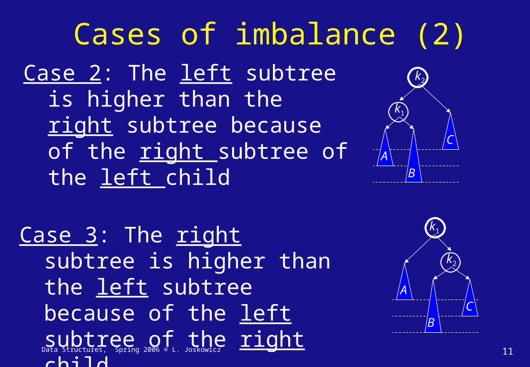
Cases of imbalance (2)Case 2: The left subtree is higher

than the right subtree because of the right subtree of the left child

Case 3: The right subtree is higher than the left subtree because of the left subtree of the right child

k2

k1

CA

B

k1

k2

CA

B


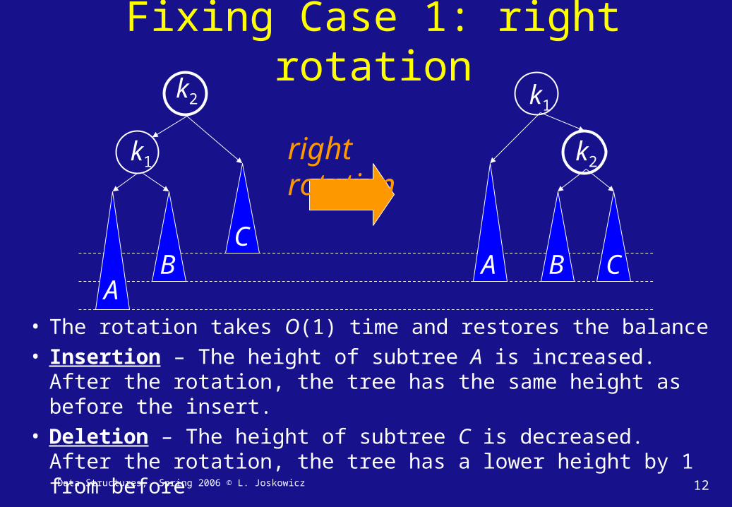
• The rotation takes O(1) time and restores the balance • Insertion – The height of subtree A is increased. After the

rotation, the tree has the same height as before the insert.• Deletion – The height of subtree C is decreased. After the

rotation, the tree has a lower height by 1 from before

Fixing Case 1: right rotationk2

k1

AB

C

right rotation k2

k1

A B C


Case 1: Insertion example

12

8 16

14104

62

1

k2

k1 C

A B

12

8

16

14

10

4

6

2

1

k2

k1

CA

B

Insert 1


Fixing Case 4: left rotation

k1

k2

CB

A

left rotation

Analysis as in Case 1

k1

k2

CBA


Case 4: deletion example

5

7

9

4

delete left rotationk1

k2

7

95

k2

k1

5

7

9

k1

k2


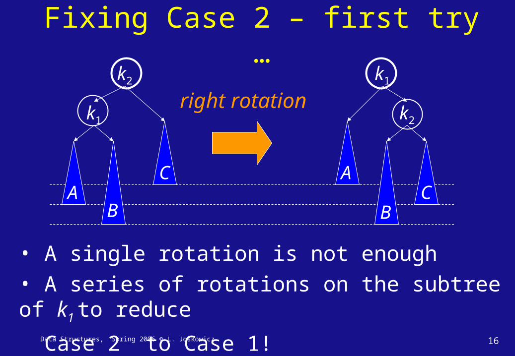
Fixing Case 2 – first try …

• A single rotation is not enough

• A series of rotations on the subtree of k1 to reduce

Case 2 to Case 1!

k2

k1

BA

C

right rotationk2

k1

B

AC


Fixing Case 2: right then left rotation

k3

k1

AC

k2

B1 B2

left rotation on k1

right rotation on k3

k3

k1

A

C

k2

B1

B2

k3k1

A C

k2

B1 B2


Case 2: insertion example

12

8 16

14104

62

5

k3

k1

C

A B1

k2

left rotation on 4

k1

12

8 16

14106

4

5

k3

C

A B1

k2

2

right rotation on 8

12

6 16

1484

52 10

k3k1

CB1

k2

A

no B2


Fixing Case 3: right then left rotation

k1

k3

CA

right rotation on k3

left rotation on k1

k2

B1 B2

Analysis as in Case 2

k3k1

A C

k2

B1 B2


Insert and delete operations (1)• Insert/delete the element as in a regular binary search

tree, and then re-balance.

• Observation: only nodes on the path from the root to the node that was changed may become unbalanced.

• Assume we go left: the right subtree was not changed, and stays balanced. This holds as we descend the tree.


Insert and delete operations (2)• After adding/deleting a leaf, go up, back to the root.

• Re-balance every node on the way as necessary.

• The path is O(lg n) long, and each node balance takes O(1), thus the total time for every operation is O(lg n).

• For the insertion we can do better: when going up, after the first balance, the subtree that was balanced has height as before, so all higher nodes are now balanced again. We can find this node in the pass down to the leaf, so one pass is enough.


Example: deletion requiring two passes

18

12 21

7

3 8

9

13

10

11

15

14 16

17

delete 3


Summary• Efficient dynamic operations on a binary tree require a

balance tree whose height is O(lg n)

• Balanced height trees:– AVL trees– Red-black trees– B-trees

• Insertion and deletion operations might require re-balancing in O(lg n) to restore balanced tree properties

• Re-balancing with left and/or right rotations on a case by case basis.

data structures – lecture balanced trees

Documents