data stream mining - department of computer …abifet/moa/streammining.pdf · data stream mining a...
TRANSCRIPT

DATA STREAMMINING
A Practical ApproachAlbert Bifet and Richard Kirkby
August 2009


Contents
I Introduction and Preliminaries 3
1 Preliminaries 51.1 MOA Stream Mining . . . . . . . . . . . . . . . . . . . . . . . . 51.2 Assumptions . . . . . . . . . . . . . . . . . . . . . . . . . . . . . 71.3 Requirements . . . . . . . . . . . . . . . . . . . . . . . . . . . . 81.4 Mining Strategies . . . . . . . . . . . . . . . . . . . . . . . . . . 101.5 Change Detection Strategies . . . . . . . . . . . . . . . . . . . . 13
2 MOA Experimental Setting 172.1 Previous Evaluation Practices . . . . . . . . . . . . . . . . . . . 19
2.1.1 Batch Setting . . . . . . . . . . . . . . . . . . . . . . . . 192.1.2 Data Stream Setting . . . . . . . . . . . . . . . . . . . . 21
2.2 Evaluation Procedures for Data Streams . . . . . . . . . . . . . 252.2.1 Holdout . . . . . . . . . . . . . . . . . . . . . . . . . . . 262.2.2 Interleaved Test-Then-Train or Prequential . . . . . . . 262.2.3 Comparison . . . . . . . . . . . . . . . . . . . . . . . . . 27
2.3 Testing Framework . . . . . . . . . . . . . . . . . . . . . . . . . 282.4 Environments . . . . . . . . . . . . . . . . . . . . . . . . . . . . 30
2.4.1 Sensor Network . . . . . . . . . . . . . . . . . . . . . . . 312.4.2 Handheld Computer . . . . . . . . . . . . . . . . . . . . 312.4.3 Server . . . . . . . . . . . . . . . . . . . . . . . . . . . . 31
2.5 Data Sources . . . . . . . . . . . . . . . . . . . . . . . . . . . . . 322.5.1 Random Tree Generator . . . . . . . . . . . . . . . . . . 332.5.2 Random RBF Generator . . . . . . . . . . . . . . . . . . 342.5.3 LED Generator . . . . . . . . . . . . . . . . . . . . . . . 342.5.4 Waveform Generator . . . . . . . . . . . . . . . . . . . . 342.5.5 Function Generator . . . . . . . . . . . . . . . . . . . . . 34
2.6 Generation Speed and Data Size . . . . . . . . . . . . . . . . . 352.7 Evolving Stream Experimental Setting . . . . . . . . . . . . . . 39
2.7.1 Concept Drift Framework . . . . . . . . . . . . . . . . . 402.7.2 Datasets for concept drift . . . . . . . . . . . . . . . . . 42
II Stationary Data Stream Learning 45
3 Hoeffding Trees 473.1 The Hoeffding Bound for Tree Induction . . . . . . . . . . . . . 483.2 The Basic Algorithm . . . . . . . . . . . . . . . . . . . . . . . . 50
3.2.1 Split Confidence . . . . . . . . . . . . . . . . . . . . . . 513.2.2 Sufficient Statistics . . . . . . . . . . . . . . . . . . . . . 513.2.3 Grace Period . . . . . . . . . . . . . . . . . . . . . . . . 523.2.4 Pre-pruning . . . . . . . . . . . . . . . . . . . . . . . . . 53
i
CONTENTS
3.2.5 Tie-breaking . . . . . . . . . . . . . . . . . . . . . . . . . 543.2.6 Skewed Split Prevention . . . . . . . . . . . . . . . . . . 55
3.3 Memory Management . . . . . . . . . . . . . . . . . . . . . . . 553.3.1 Poor Attribute Removal . . . . . . . . . . . . . . . . . . 60
3.4 MOA Java Implementation Details . . . . . . . . . . . . . . . . 603.4.1 Fast Size Estimates . . . . . . . . . . . . . . . . . . . . . 63
4 Numeric Attributes 654.1 Batch Setting Approaches . . . . . . . . . . . . . . . . . . . . . 66
4.1.1 Equal Width . . . . . . . . . . . . . . . . . . . . . . . . . 674.1.2 Equal Frequency . . . . . . . . . . . . . . . . . . . . . . 674.1.3 k-means Clustering . . . . . . . . . . . . . . . . . . . . . 674.1.4 Fayyad and Irani . . . . . . . . . . . . . . . . . . . . . . 684.1.5 C4.5 . . . . . . . . . . . . . . . . . . . . . . . . . . . . . . 68
4.2 Data Stream Approaches . . . . . . . . . . . . . . . . . . . . . . 694.2.1 VFML Implementation . . . . . . . . . . . . . . . . . . . 704.2.2 Exhaustive Binary Tree . . . . . . . . . . . . . . . . . . . 714.2.3 Quantile Summaries . . . . . . . . . . . . . . . . . . . . 724.2.4 Gaussian Approximation . . . . . . . . . . . . . . . . . 734.2.5 Numerical Interval Pruning . . . . . . . . . . . . . . . . 77
5 Prediction Strategies 795.1 Majority Class . . . . . . . . . . . . . . . . . . . . . . . . . . . . 795.2 Naive Bayes Leaves . . . . . . . . . . . . . . . . . . . . . . . . . 795.3 Adaptive Hybrid . . . . . . . . . . . . . . . . . . . . . . . . . . 82
6 Hoeffding Tree Ensembles 856.1 Batch Setting . . . . . . . . . . . . . . . . . . . . . . . . . . . . . 89
6.1.1 Bagging . . . . . . . . . . . . . . . . . . . . . . . . . . . 896.1.2 Boosting . . . . . . . . . . . . . . . . . . . . . . . . . . . 906.1.3 Option Trees . . . . . . . . . . . . . . . . . . . . . . . . . 95
6.2 Data Stream Setting . . . . . . . . . . . . . . . . . . . . . . . . . 976.2.1 Bagging . . . . . . . . . . . . . . . . . . . . . . . . . . . 976.2.2 Boosting . . . . . . . . . . . . . . . . . . . . . . . . . . . 986.2.3 Option Trees . . . . . . . . . . . . . . . . . . . . . . . . . 101
6.3 Realistic Ensemble Sizes . . . . . . . . . . . . . . . . . . . . . . 106
III Evolving Data Stream Learning 109
7 Evolving data streams 1117.1 Algorithms for mining with change . . . . . . . . . . . . . . . 112
7.1.1 OLIN: Last . . . . . . . . . . . . . . . . . . . . . . . . . . 1127.1.2 CVFDT: Domingos . . . . . . . . . . . . . . . . . . . . . 1127.1.3 UFFT: Gama . . . . . . . . . . . . . . . . . . . . . . . . . 113
7.2 A Methodology for Adaptive Stream Mining . . . . . . . . . . 115
ii

CONTENTS
7.2.1 Time Change Detectors and Predictors: A General Frame-work . . . . . . . . . . . . . . . . . . . . . . . . . . . . . 116
7.2.2 Window Management Models . . . . . . . . . . . . . . 1187.3 Optimal Change Detector and Predictor . . . . . . . . . . . . . 120
8 Adaptive Sliding Windows 1218.1 Introduction . . . . . . . . . . . . . . . . . . . . . . . . . . . . . 1218.2 Maintaining Updated Windows of Varying Length . . . . . . . 122
8.2.1 Setting . . . . . . . . . . . . . . . . . . . . . . . . . . . . 1228.2.2 First algorithm: ADWIN0 . . . . . . . . . . . . . . . . . 1228.2.3 ADWIN0 for Poisson processes . . . . . . . . . . . . . . 1278.2.4 Improving time and memory requirements . . . . . . . 128
8.3 K-ADWIN = ADWIN + Kalman Filtering . . . . . . . . . . . . . . 132
9 Adaptive Hoeffding Trees 1359.1 Introduction . . . . . . . . . . . . . . . . . . . . . . . . . . . . . 1359.2 Decision Trees on Sliding Windows . . . . . . . . . . . . . . . . 136
9.2.1 HWT-ADWIN : Hoeffding Window Tree using ADWIN . 1369.2.2 CVFDT . . . . . . . . . . . . . . . . . . . . . . . . . . . . 139
9.3 Hoeffding Adaptive Trees . . . . . . . . . . . . . . . . . . . . . 1409.3.1 Example of performance Guarantee . . . . . . . . . . . 1419.3.2 Memory Complexity Analysis . . . . . . . . . . . . . . 142
10 Adaptive Ensemble Methods 14310.1 New method of Bagging using trees of different size . . . . . . 14310.2 New method of Bagging using ADWIN . . . . . . . . . . . . . . 14610.3 Adaptive Hoeffding Option Trees . . . . . . . . . . . . . . . . . 14710.4 Method performance . . . . . . . . . . . . . . . . . . . . . . . . 147
Bibliography 149
iii


Introduction
Massive Online Analysis (MOA) is a software environment for implement-ing algorithms and running experiments for online learning from evolvingdata streams.
MOA includes a collection of offline and online methods as well as toolsfor evaluation. In particular, it implements boosting, bagging, and Hoeffd-ing Trees, all with and without Naıve Bayes classifiers at the leaves.
MOA is related to WEKA, the Waikato Environment for Knowledge Anal-ysis, which is an award-winning open-source workbench containing imple-mentations of a wide range of batch machine learning methods. WEKA isalso written in Java. The main benefits of Java are portability, where applica-tions can be run on any platform with an appropriate Java virtual machine,and the strong and well-developed support libraries. Use of the language iswidespread, and features such as the automatic garbage collection help toreduce programmer burden and error.
This text explains the theoretical and practical foundations of the meth-ods and streams available in MOA. The moa and the weka are both birds na-tive to New Zealand. The weka is a cheeky bird of similar size to a chicken.The moa was a large ostrich-like bird, an order of magnitude larger than aweka, that was hunted to extinction.


Part I
Introduction and Preliminaries
3


1Preliminaries
In today’s information society, extraction of knowledge is becoming a veryimportant task for many people. We live in an age of knowledge revolution.Peter Drucker [42], an influential management expert, writes “From nowon, the key is knowledge. The world is not becoming labor intensive, notmaterial intensive, not energy intensive, but knowledge intensive”. Thisknowledge revolution is based in an economic change from adding value byproducing things which is, ultimately limited, to adding value by creatingand using knowledge which can grow indefinitely.
The digital universe in 2007 was estimated in [64] to be 281 exabytes or281 billion gigabytes, and by 2011, the digital universe will be 10 times thesize it was 5 years before. The amount of information created, or capturedexceeded available storage for the first time in 2007.
To deal with these huge amount of data in a responsible way, green com-puting is becoming a necessity. Green computing is the study and practice ofusing computing resources efficiently. A main approach to green comput-ing is based on algorithmic efficiency. The amount of computer resourcesrequired for any given computing function depends on the efficiency of thealgorithms used. As the cost of hardware has declined relative to the cost ofenergy, the energy efficiency and environmental impact of computing sys-tems and programs are receiving increased attention.
1.1 MOA Stream Mining
A largely untested hypothesis of modern society is that it is important torecord data as it may contain valuable information. This occurs in almostall facets of life from supermarket checkouts to the movements of cows ina paddock. To support the hypothesis, engineers and scientists have pro-duced a raft of ingenious schemes and devices from loyalty programs toRFID tags. Little thought however, has gone into how this quantity of datamight be analyzed.
Machine learning, the field for finding ways to automatically extract infor-mation from data, was once considered the solution to this problem. Histor-ically it has concentrated on learning from small numbers of examples, be-cause only limited amounts of data were available when the field emerged.Some very sophisticated algorithms have resulted from the research that
5

CHAPTER 1. PRELIMINARIES
can learn highly accurate models from limited training examples. It is com-monly assumed that the entire set of training data can be stored in workingmemory.
More recently the need to process larger amounts of data has motivatedthe field of data mining. Ways are investigated to reduce the computationtime and memory needed to process large but static data sets. If the datacannot fit into memory, it may be necessary to sample a smaller training set.Alternatively, algorithms may resort to temporary external storage, or onlyprocess subsets of data at a time. Commonly the goal is to create a learningprocess that is linear in the number of examples. The essential learningprocedure is treated like a scaled up version of classic machine learning,where learning is considered a single, possibly expensive, operation—a setof training examples are processed to output a final static model.
The data mining approach may allow larger data sets to be handled, butit still does not address the problem of a continuous supply of data. Typi-cally, a model that was previously induced cannot be updated when newinformation arrives. Instead, the entire training process must be repeatedwith the new examples included. There are situations where this limitationis undesirable and is likely to be inefficient.
The data stream paradigm has recently emerged in response to the contin-uous data problem. Algorithms written for data streams can naturally copewith data sizes many times greater than memory, and can extend to chal-lenging real-time applications not previously tackled by machine learningor data mining. The core assumption of data stream processing is that train-ing examples can be briefly inspected a single time only, that is, they arrivein a high speed stream, then must be discarded to make room for subse-quent examples. The algorithm processing the stream has no control overthe order of the examples seen, and must update its model incrementally aseach example is inspected. An additional desirable property, the so-calledanytime property, requires that the model is ready to be applied at any pointbetween training examples.
Studying purely theoretical advantages of algorithms is certainly usefuland enables new developments, but the demands of data streams requirethis to be followed up with empirical evidence of performance. Claimingthat an algorithm is suitable for data stream scenarios implies that it pos-sesses the necessary practical capabilities. Doubts remain if these claimscannot be backed by reasonable empirical evidence.
Data stream classification algorithms require appropriate and completeevaluation practices. The evaluation should allow users to be sure that par-ticular problems can be handled, to quantify improvements to algorithms,and to determine which algorithms are most suitable for their problem.MOA is suggested with these needs in mind.
Measuring data stream classification performance is a three dimensionalproblem involving processing speed, memory and accuracy. It is not possi-ble to enforce and simultaneously measure all three at the same time so inMOA it is necessary to fix the memory size and then record the other two.
6

1.2. ASSUMPTIONS
Various memory sizes can be associated with data stream application sce-narios so that basic questions can be asked about expected performance ofalgorithms in a given application scenario. MOA is developed to provideuseful insight about classification performance.
1.2 Assumptions
MOA is concerned with the problem of classification, perhaps the most com-monly researched machine learning task. The goal of classification is to pro-duce a model that can predict the class of unlabeled examples, by trainingon examples whose label, or class, is supplied. To clarify the problem settingbeing addressed, several assumptions are made about the typical learningscenario:
1. The data is assumed to have a small and fixed number of columns, orattributes/features—several hundred at the most.
2. The number of rows, or examples, is very large—millions of examplesat the smaller scale. In fact, algorithms should have the potential toprocess an infinite amount of data, meaning that they will not exceedmemory limits or otherwise fail no matter how many training exam-ples are processed.
3. The data has a limited number of possible class labels, typically lessthan ten.
4. The amount of memory available to a learning algorithm depends onthe application. The size of the training data will be considerablylarger than the available memory.
5. There should be a small upper bound on the time allowed to trainor classify an example. This permits algorithms to scale linearly withthe number of examples, so users can process N times more than anexisting amount simply by waiting N times longer than they alreadyhave.
6. Stream concepts are assumed to be stationary or evolving. Conceptdrift occurs when the underlying concept defining the target beinglearned begins to shift over time.
The first three points emphasize that the aim is to scale with the num-ber of examples. Data sources that are large in other dimensions, such asnumbers of attributes or possible labels are not the intended problem do-main. Points 4 and 5 outline what is needed from a solution. Regardingpoint 6, some researchers argue that addressing concept drift is one of themost crucial issues in processing data streams.
7
CHAPTER 1. PRELIMINARIES
1.3 Requirements
The conventional machine learning setting, referred to in this text as thebatch setting, operates assuming that the training data is available as a wholeset—any example can be retrieved as needed for little cost. An alternativeis to treat the training data as a stream, a potentially endless flow of datathat arrives in an order that cannot be controlled. Note that an algorithmcapable of learning from a stream is, by definition, a data mining algorithm.
Placing classification in a data stream setting offers several advantages.Not only is the limiting assumption of early machine learning techniquesaddressed, but other applications even more demanding than mining oflarge databases can be attempted. An example of such an application isthe monitoring of high-speed network traffic, where the unending flow ofdata is too overwhelming to consider storing and revisiting.
A classification algorithm must meet several requirements in order towork with the assumptions and be suitable for learning from data streams.The requirements, numbered 1 through 4, are detailed below.
Requirement 1: Process an example at a time, and inspect itonly once (at most)
The key characteristic of a data stream is that data ‘flows’ by one exam-ple after another. There is no allowance for random access of the data beingsupplied. Each example must be accepted as it arrives in the order that itarrives. Once inspected or ignored, an example is discarded with no abilityto retrieve it again.
Although this requirement exists on the input to an algorithm, there isno rule preventing an algorithm from remembering examples internally inthe short term. An example of this may be the algorithm storing up a batchof examples for use by a conventional learning scheme. While the algorithmis free to operate in this manner, it will have to discard stored examples atsome point if it is to adhere to requirement 2.
The inspect-once rule may only be relaxed in cases where it is practicalto re-send the entire stream, equivalent to multiple scans over a database.In this case an algorithm may be given a chance during subsequent passesto refine the model it has learned. However, an algorithm that requires anymore than a single pass to operate is not flexible enough for universal ap-plicability to data streams.
Requirement 2: Use a limited amount of memory
The main motivation for employing the data stream model is that it allowsprocessing of data that is many times larger than available working mem-ory. The danger with processing such large amounts of data is that memoryis easily exhausted if there is no intentional limit set on its use.
8

1.3. REQUIREMENTS
Memory used by an algorithm can be divided into two categories: mem-ory used to store running statistics, and memory used to store the currentmodel. For the most memory-efficient algorithm they will be one and thesame, that is, the running statistics directly constitute the model used forprediction.
This memory restriction is a physical restriction that can only be relaxedif external storage is used, temporary files for example. Any such work-around needs to be done with consideration of requirement 3.
Requirement 3: Work in a limited amount of time
For an algorithm to scale comfortably to any number of examples, its run-time complexity must be linear in the number of examples. This can beachieved in the data stream setting if there is a constant, preferably small,upper bound on the amount of processing per example.
Furthermore, if an algorithm is to be capable of working in real-time, itmust process the examples as fast if not faster than they arrive. Failure todo so inevitably means loss of data.
Absolute timing is not as critical in less demanding applications, suchas when the algorithm is being used to classify a large but persistent datasource. However, the slower the algorithm is, the less value it will be forusers who require results within a reasonable amount of time.
Requirement 4: Be ready to predict at any point
An ideal algorithm should be capable of producing the best model it canfrom the data it has observed after seeing any number of examples. In prac-tice it is likely that there will be periods where the model stays constant,such as when a batch based algorithm is storing up the next batch.
The process of generating the model should be as efficient as possible,the best case being that no translation is necessary. That is, the final model isdirectly manipulated in memory by the algorithm as it processes examples,rather than having to recompute the model based on running statistics.
The data stream classification cycle
Figure 1.1 illustrates the typical use of a data stream classification algorithm,and how the requirements fit in. The general model of data stream classifi-cation follows these three steps in a repeating cycle:
1. The algorithm is passed the next available example from the stream(requirement 1).
2. The algorithm processes the example, updating its data structures. Itdoes so without exceeding the memory bounds set on it (requirement2), and as quickly as possible (requirement 3).
9

CHAPTER 1. PRELIMINARIES
3 modelrequirement 4
2 learningrequirements 2 & 3
1 inputrequirement 1
examplestraining
examplestest
predictions
Figure 1.1: The data stream classification cycle.
3. The algorithm is ready to accept the next example. On request it isable to supply a model that can be used to predict the class of unseenexamples (requirement 4).
1.4 Mining Strategies
The task of modifying machine learning algorithms to handle large datasets is known as scaling up [34]. Analogous to approaches used in data min-ing, there are two general strategies for taking machine learning conceptsand applying them to data streams. The wrapper approach aims at maxi-mum reuse of existing schemes, whereas adaptation looks for new methodstailored to the data stream setting.
Using a wrapper approach means that examples must in some way becollected into a batch so that a traditional batch learner can be used to in-duce a model. The models must then be chosen and combined in some wayto form predictions. The difficulties of this approach include determiningappropriate training set sizes, and also that training times will be out of thecontrol of a wrapper algorithm, other than the indirect influence of adjust-ing the training set size. When wrapping around complex batch learners,training sets that are too large could stall the learning process and preventthe stream from being processed at an acceptable speed. Training sets thatare too small will induce models that are poor at generalizing to new ex-
10

1.4. MINING STRATEGIES
amples. Memory management of a wrapper scheme can only be conductedon a per-model basis, where memory can be freed by forgetting some of themodels that were previously induced. Examples of wrapper approachesfrom the literature include Wang et al. [153], Street and Kim [145] and Chuand Zaniolo [29].
Purposefully adapted algorithms designed specifically for data streamproblems offer several advantages over wrapper schemes. They can exertgreater control over processing times per example, and can conduct mem-ory management at a finer-grained level. Common varieties of machinelearning approaches to classification fall into several general classes. Theseclasses of method are discussed below, along with their potential for adap-tation to data streams:
decision trees This class of method is the main focus of the text . Chapter 3studies a successful adaptation of decision trees to data streams [39]and outlines the motivation for this choice.
rules Rules are somewhat similar to decision trees, as a decision tree canbe decomposed into a set of rules, although the structure of a rule setcan be more flexible than the hierarchy of a tree. Rules have an ad-vantage that each rule is a disjoint component of the model that canbe evaluated in isolation and removed from the model without majordisruption, compared to the cost of restructuring decision trees. How-ever, rules may be less efficient to process than decision trees, whichcan guarantee a single decision path per example. Ferrer-Troyano etal. [47, 48] have developed methods for inducing rule sets directlyfrom streams.
lazy/nearest neighbour This class of method is described as lazy because inthe batch learning setting no work is done during training, but all ofthe effort in classifying examples is delayed until predictions are re-quired. The typical nearest neighbour approach will look for examplesin the training set that are most similar to the example being classified,as the class labels of these examples are expected to be a reasonableindicator of the unknown class. The challenge with adapting thesemethods to the data stream setting is that training can not afford to belazy, because it is not possible to store the entire training set. Insteadthe examples that are remembered must be managed so that they fitinto limited memory. An intuitive solution to this problem involvesfinding a way to merge new examples with the closest ones alreadyin memory, the main question being what merging process will per-form best. Another issue is that searching for the nearest neighboursis costly. This cost may be reduced by using efficient data structuresdesigned to reduce search times. Nearest neighbour based methodsare a popular research topic for data stream classification. Examplesof systems include [109, 55, 98, 13].
11

CHAPTER 1. PRELIMINARIES
support vector machines/neural networks Both of these methods are re-lated and of similar power, although support vector machines [26] areinduced via an alternate training method and are a hot research topicdue to their flexibility in allowing various kernels to offer tailored so-lutions. Memory management for support vector machines could bebased on limiting the number of support vectors being induced. In-cremental training of support vector machines has been explored pre-viously, for example [146]. Neural networks are relatively straightfor-ward to train on a data stream. A real world application using neuralnetworks is given by Gama and Rodrigues [63]. The typical procedureassumes a fixed network, so there is no memory management prob-lem. It is straightforward to use the typical backpropagation trainingmethod on a stream of examples, rather than repeatedly scanning afixed training set as required in the batch setting.
Bayesian methods These methods are based around Bayes’ theorem and com-pute probabilities in order to perform Bayesian inference. The simplestBayesian method, Naive Bayes, is described in Section 5.2, and is aspecial case of algorithm that needs no adaptation to data streams.This is because it is straightforward to train incrementally and doesnot add structure to the model, so that memory usage is small andbounded. A single Naive Bayes model will generally not be as ac-curate as more complex models. The more general case of Bayesiannetworks is also suited to the data stream setting, at least when thestructure of the network is known. Learning a suitable structure forthe network is a more difficult problem. Hulten and Domingos [87]describe a method of learning Bayesian networks from data streamsusing Hoeffding bounds. Bouckaert [16] also presents a solution.
meta/ensemble methods These methods wrap around other existing meth-ods, typically building up an ensemble of models. Examples of thisinclude [127, 109]. This is the other major class of algorithm studiedin-depth by this text , beginning in Chapter 6.
Gaber et al. [56] survey the field of data stream classification algorithmsand list those that they believe are major contributions. Most of these havealready been covered: Domingos and Hulten’s VFDT [39], the decision treealgorithm studied in-depth by this text ; ensemble-based classification by Wanget al. [153] that has been mentioned as a wrapper approach; SCALLOP, arule-based learner that is the earlier work of Ferrer-Troyano et al. [47]; AN-NCAD, which is a nearest neighbour method developed by Law and Zan-iolo [109] that operates using Haar wavelet transformation of data and smallclassifier ensembles; and LWClass proposed by Gaber et al. [55], anothernearest neighbour based technique, that actively adapts to fluctuating timeand space demands by varying a distance threshold. The other methodsin their survey that have not yet been mentioned include on demand classifi-cation. This method by Aggarwal et al. [1] performs dynamic collection of
12

1.5. CHANGE DETECTION STRATEGIES
training examples into supervised micro-clusters. From these clusters, a near-est neighbour type classification is performed, where the goal is to quicklyadapt to concept drift. The final method included in the survey is knownas an online information network (OLIN) proposed by Last [108]. This methodhas a strong focus on concept drift, and uses a fuzzy technique to construct amodel similar to decision trees, where the frequency of model building andtraining window size is adjusted to reduce error as concepts evolve.
Dealing with time-changing data requires strategies for detecting andquantifying change, forgetting stale examples, and for model revision. Fairlygeneric strategies exist for detecting change and deciding when examplesare no longer relevant.
1.5 Change Detection Strategies
The following different modes of change have been identified in the litera-ture [147, 144, 157]:
• concept change
– concept drift
– concept shift
• distribution or sampling change
Concept refers to the target variable, which the model is trying to predict.Concept change is the change of the underlying concept over time. Conceptdrift describes a gradual change of the concept and concept shift happenswhen a change between two concepts is more abrupt.
Distribution change, also known as sampling change or shift or virtualconcept drift , refers to the change in the data distribution. Even if the con-cept remains the same, the change may often lead to revising the currentmodel as the model’s error rate may no longer be acceptable with the newdata distribution.
Some authors, as Stanley [144], have suggested that from the practicalpoint of view, it is not essential to differentiate between concept change andsampling change since the current model needs to be changed in both cases.
Change detection is not an easy task, since a fundamental limitation ex-ists [72]: the design of a change detector is a compromise between detectingtrue changes and avoiding false alarms. See [72, 12] for more detailed sur-veys of change detection methods.
The CUSUM Test
The cumulative sum (CUSUM algorithm), first proposed in [128], is a changedetection algorithm that gives an alarm when the mean of the input data issignificantly different from zero. The CUSUM input εt can be any filterresidual, for instance the prediction error from a Kalman filter.
13

CHAPTER 1. PRELIMINARIES
The CUSUM test is as follows:
g0 = 0
gt = max (0, gt−1 + εt − υ)
if gt > h then alarm and gt = 0
The CUSUM test is memoryless, and its accuracy depends on the choice ofparameters υ and h.
The Geometric Moving Average Test
The CUSUM test is a stopping rule. Other stopping rules exist. For example,the Geometric Moving Average (GMA) test, first proposed in [134], is thefollowing
g0 = 0
gt = λgt−1 + (1− λ)εt
if gt > h then alarm and gt = 0
The forgetting factor λ is used to give more or less weight to the last dataarrived. The treshold h is used to tune the sensitivity and false alarm rate ofthe detector.
Statistical Tests
CUSUM and GMA are methods for dealing with numeric sequences. Formore complex populations, we need to use other methods. There exist somestatistical tests that may be used to detect change. A statistical test is a pro-cedure for deciding whether a hypothesis about a quantitative feature of apopulation is true or false. We test an hypothesis of this sort by drawing arandom sample from the population in question and calculating an appro-priate statistic on its items. If, in doing so, we obtain a value of the statisticthat would occur rarely when the hypothesis is true, we would have reasonto reject the hypothesis.
To detect change, we need to compare two sources of data, and decide ifthe hypothesis H0 that they come from the same distribution is true. Let’ssuppose we have two estimates, µ0 and µ1 with variances σ20 and σ21. If thereis no change in the data, these estimates will be consistent. Otherwise, ahypothesis test will reject H0 and a change is detected. There are severalways to construct such a hypothesis test. The simplest one is to study thedifference
µ0 − µ1 ∈ N(0, σ20 + σ21), under H0
or, to make a χ2 test
(µ0 − µ1)2
σ20 + σ21∈ χ2(1), under H0
14

1.5. CHANGE DETECTION STRATEGIES
from which a standard hypothesis test can be formulated.For example, suppose we want to design a change detector using a sta-
tistical test with a probability of false alarm of 5%, that is,
Pr
(|µ0 − µ1|√σ20 + σ21
> h
)= 0.05
A table of the Gaussian distribution shows that P(X < 1.96) = 0.975, sothe test becomes
(µ0 − µ1)2
σ20 + σ21> 1.96
Note that this test uses the normality hypothesis. In Chapter 8 we will pro-pose a similar test with theoretical guarantees. However, we could haveused this test on the methods of Chapter 8.
The Kolmogorov-Smirnov test [94] is another statistical test used to com-pare two populations. Given samples from two populations, the cumulativedistribution functions can be determined and plotted. Hence the maximumvalue of the difference between the plots can be found and compared witha critical value. If the observed value exceeds the critical value, H0 is re-jected and a change is detected. It is not obvious how to implement theKolmogorov-Smirnov test dealing with data streams. Kifer et al. [99] pro-pose a KS-structure to implement Kolmogorov-Smirnov and similar tests,on the data stream setting.
Drift Detection Method
The drift detection method (DDM) proposed by Gama et al. [57] controls thenumber of errors produced by the learning model during prediction. It com-pares the statistics of two windows: the first one contains all the data, andthe second one contains only the data from the beginning until the numberof errors increases. This method does not store these windows in memory.It keeps only statistics and a window of recent data.
The number of errors in a sample of n examples is modelized by a bino-mial distribution. For each point i in the sequence that is being sampled, theerror rate is the probability of misclassifying (pi), with standard deviationgiven by si =
√pi(1− pi)/i. It assumes (as can be argued e.g. in the PAC
learning model [120]) that the error rate of the learning algorithm (pi) willdecrease while the number of examples increases if the distribution of theexamples is stationary. A significant increase in the error of the algorithm,suggests that the class distribution is changing and, hence, the actual deci-sion model is supposed to be inappropriate. Thus, it stores the values of piand si when pi+si reaches its minimum value during the process (obtainingppmin and smin), and when the following conditions triggers:
• pi + si ≥ pmin + 2 · smin for the warning level. Beyond this level, theexamples are stored in anticipation of a possible change of context.
15

CHAPTER 1. PRELIMINARIES
• pi+si ≥ pmin+3 ·smin for the drift level. Beyond this level the conceptdrift is supposed to be true, the model induced by the learning methodis reset and a new model is learnt using the examples stored since thewarning level triggered. The values for pmin and smin are reset too.
This approach has a good behaviour of detecting abrupt changes andgradual changes when the gradual change is not very slow, but it has diffi-culties when the change is slowly gradual. In that case, the examples willbe stored for long time, the drift level can take too much time to trigger andthe example memory can be exceeded.
Baena-Garcıa et al. proposed a new method EDDM in order to improveDDM. EDDM [10] is shown to be better than DDM for some data sets andworse for others. It is based on the estimated distribution of the distancesbetween classification errors. The window resize procedure is governed bythe same heuristics.
Exponential Weighted Moving Average
An Estimator is an algorithm that estimates the desired statistics on the in-put data, which may change over time. The simplest Estimator algorithmfor the expected is the linear estimator, which simply returns the average ofthe data items contained in the Memory. Other examples of run-time ef-ficient estimators are Auto-Regressive, Auto Regressive Moving Average,and Kalman filters.
An exponentially weighted moving average (EWMA) estimator is an al-gorithm that updates the estimation of a variable by combining the mostrecent measurement of the variable with the EWMA of all previous mea-surements:
Xt = αzt + (1− α)Xt−1 = Xt−1 + α(zt − Xt−1)
where Xt is the moving average, zt is the latest measurement, and α is theweight given to the latest measurement (between 0 and 1). The idea is toproduce an estimate that gives more weight to recent measurements, onthe assumption that recent measurements are more likely to be relevant.Choosing an adequate α is a difficult problem, and it is not trivial.
16

2MOA Experimental Setting
This chapter establishes the settings under which stream mining experi-ments may be conducted, presenting the framework MOA to place variouslearning algorithms under test. This experimental methodology is moti-vated by the requirements of the end user and their desired application.
Figure 2.1: Graphical user interface of MOA
A user wanting to classify examples in a stream of data will have a set ofrequirements. They will have a certain volume of data, composed of a num-ber of features per example, and a rate at which examples arrive. They willhave the computing hardware on which the training of the model and theclassification of new examples is to occur. Users will naturally seek the mostaccurate predictions possible on the hardware provided. They are, however,more likely to accept a solution that sacrifices accuracy in order to function,than no solution at all. Within reason the user’s requirements may be re-laxed, such as reducing the training features or upgrading the hardware,but there comes a point at which doing so would be unsatisfactory.
The behaviour of a data stream learning algorithm has three dimensionsof interest—the amount of space (computer memory) required, the time re-quired to learn from training examples and to predict labels for new exam-ples, and the error of the predictions. When the user’s requirements cannotbe relaxed any further, the last remaining element that can be tuned to meet
17

CHAPTER 2. MOA EXPERIMENTAL SETTING
the demands of the problem is the effectiveness of the learning algorithm—the ability of the algorithm to output minimum error in limited time andspace.
The error of an algorithm is the dimension that people would like to con-trol the most, but it is the least controllable. The biggest factors influencingerror are the representational power of the algorithm, how capable the modelis at capturing the true underlying concept in the stream, and its generaliza-tion power, how successfully it can ignore noise and isolate useful patternsin the data.
Adjusting the time and space used by an algorithm can influence error.Time and space are interdependent. By storing more pre-computed infor-mation, such as look up tables, an algorithm can run faster at the expenseof space. An algorithm can also run faster by processing less information,either by stopping early or storing less, thus having less data to process.The more time an algorithm has to process, or the more information that isprocessed, the more likely it is that error can be reduced.
The time and space requirements of an algorithm can be controlled bydesign. The algorithm can be optimised to reduce memory footprint andruntime. More directly, an algorithm can be made aware of the resourcesit is using and dynamically adjust. For example, an algorithm can take amemory limit as a parameter, and take steps to obey the limit. Similarly, itcould be made aware of the time it is taking, and scale computation back toreach a time goal.
The easy way to limit either time or space is to stop once the limit isreached, and resort to the best available output at that point. For a timelimit, continuing to process will require the user to wait longer, a compro-mise that may be acceptable in some situations. For a space limit, the onlyway to continue processing is to have the algorithm specifically designed todiscard some of its information, hopefully information that is least impor-tant. Additionally, time is highly dependent on physical processor imple-mentation, whereas memory limits are universal. The space requirement isa hard overriding limit that is ultimately dictated by the hardware available.An algorithm that requests more memory than is available will cease tofunction, a consequence that is much more serious than either taking longer,or losing accuracy, or both.
It follows that the space dimension should be fixed in order to evaluatealgorithmic performance. Accordingly, to evaluate the ability of an algo-rithm to meet user requirements, a memory limit is set, and the resultingtime and error performance of the algorithm is measured on a data stream.Different memory limits have been chosen to gain insight into general per-formance of algorithmic variations by covering a range of plausible situa-tions.
Several elements are covered in order to establish the evaluation frame-work used in this text. Evaluation methods already established in the fieldare surveyed in Section 2.1. Possible procedures are compared in 2.2 and thefinal evaluation framework is described in Section 2.3. The memory limits
18

2.1. PREVIOUS EVALUATION PRACTICES
used for testing are motivated in Section 2.4, and Section 2.5 describes thedata streams used for testing. Finally, Section 2.6 analyzes the speeds andsizes of the data streams involved. The particular algorithms under exami-nation are the focus of the remainder of the text.
2.1 Previous Evaluation Practices
This section assumes that the critical variable being measured by evaluationprocesses is the accuracy of a learning algorithm. Accuracy, or equivalentlyits converse, error, may not be the only concern, but it is usually the mostpertinent one. Accuracy is typically measured as the percentage of correctclassifications that a model makes on a given set of data, the most accuratelearning algorithm is the one that makes the fewest mistakes when predict-ing labels of examples. With classification problems, achieving the highestpossible accuracy is the most immediate and obvious goal. Having a reli-able estimate of accuracy enables comparison of different methods, so thatthe best available method for a given problem can be determined.
It is very optimistic to measure the accuracy achievable by a learner onthe same data that was used to train it, because even if a model achievesperfect accuracy on its training data this may not reflect the accuracy thatcan be expected on unseen data—its generalization accuracy. For the evalua-tion of a learning algorithm to measure practical usefulness, the algorithm’sability to generalize to previously unseen examples must be tested. A modelis said to overfit the data if it tries too hard to explain the training data, whichis typically noisy, so performs poorly when predicting the class label of ex-amples it has not seen before. One of the greatest challenges of machinelearning is finding algorithms that can avoid the problem of overfitting.
2.1.1 Batch Setting
Previous work on the problem of evaluating batch learning has concen-trated on making the best use of a limited supply of data. When the numberof examples available to describe a problem is in the order of hundreds oreven less then reasons for this concern are obvious. When data is scarce, ide-ally all data that is available should be used to train the model, but this willleave no remaining examples for testing. The following methods discussedare those that have in the past been considered most suitable for evaluat-ing batch machine learning algorithms, and are studied in more detail byKohavi [102].
The holdout method divides the available data into two subsets that aremutually exclusive. One of the sets is used for training, the training set,and the remaining examples are used for testing, the test or holdout set.Keeping these sets separate ensures that generalization performance is be-ing measured. Common size ratios of the two sets used in practice are 1/2training and 1/2 test, or 2/3 training and 1/3 test. Because the learner is
19

CHAPTER 2. MOA EXPERIMENTAL SETTING
not provided the full amount of data for training, assuming that it will im-prove given more data, the performance estimate will be pessimistic. Themain criticism of the holdout method in the batch setting is that the datais not used efficiently, as many examples may never be used to train thealgorithm. The accuracy estimated from a single holdout can vary greatlydepending on how the sets are divided. To mitigate this effect, the pro-cess of random subsampling will perform multiple runs of the holdout pro-cedure, each with a different random division of the data, and average theresults. Doing so also enables measurement of the accuracy estimate’s vari-ance. Unfortunately this procedure violates the assumption that the train-ing and test set are independent—classes over-represented in one set will beunder-represented in the other, which can skew the results.
In contrast to the holdout method, cross-validation maximizes the use ofexamples for both training and testing. In k-fold cross-validation the data israndomly divided into k independent and approximately equal-sized folds.The evaluation process repeats k times, each time a different fold acts asthe holdout set while the remaining folds are combined and used for train-ing. The final accuracy estimate is obtained by dividing the total numberof correct classifications by the total number of examples. In this procedureeach available example is used k − 1 times for training and exactly oncefor testing. This method is still susceptible to imbalanced class distributionbetween folds. Attempting to reduce this problem, stratified cross-validationdistributes the labels evenly across the folds to approximately reflect thelabel distribution of the entire data. Repeated cross-validation repeats thecross-validation procedure several times, each with a different random par-titioning of the folds, allowing the variance of the accuracy estimate to bemeasured.
The leave-one-out evaluation procedure is a special case of cross-validationwhere every fold contains a single example. This means with a data set of nexamples that n-fold cross validation is performed, such that n models areinduced, each of which is tested on the single example that was held out.In special situations where learners can quickly be made to ‘forget’ a sin-gle training example this process can be performed efficiently, otherwise inmost cases this procedure is expensive to perform. The leave-one-out pro-cedure is attractive because it is completely deterministic and not subject torandom effects in dividing folds. However, stratification is not possible andit is easy to construct examples where leave-one-out fails in its intended taskof measuring generalization accuracy. Consider what happens when evalu-ating using completely random data with two classes and an equal numberof examples per class—the best an algorithm can do is predict the majorityclass, which will always be incorrect on the example held out, resulting inan accuracy of 0%, even though the expected estimate should be 50%.
An alternative evaluation method is the bootstrap method introduced byEfron [43]. This method creates a bootstrap sample of a data set by samplingwith replacement a training data set of the same size as the original. Underthe process of sampling with replacement the probability that a particular
20

2.1. PREVIOUS EVALUATION PRACTICES
example will be chosen is approximately 0.632, so the method is commonlyknown as the 0.632 bootstrap. All examples not present in the training setare used for testing, which will contain on average about 36.8% of the ex-amples. The method compensates for lack of unique training examples bycombining accuracies measured on both training and test data to reach afinal estimate:
accuracybootstrap = 0.632× accuracytest + 0.368× accuracytrain (2.1)
As with the other methods, repeated random runs can be averaged to in-crease the reliability of the estimate. This method works well for very smalldata sets but suffers from problems that can be illustrated by the same sit-uation that causes problems with leave-one-out, a completely random two-class data set—Kohavi [102] argues that although the true accuracy of anymodel can only be 50%, a classifier that memorizes the training data canachieve accuracytrain of 100%, resulting in accuracybootstrap = 0.632 ×50% + 0.368 × 100% = 68.4%. This estimate is more optimistic than theexpected result of 50%.
Having considered the various issues with evaluating performance inthe batch setting, the machine learning community has settled on stratifiedten-fold cross-validation as the standard evaluation procedure, as recom-mended by Kohavi [102]. For increased reliability, ten repetitions of ten-fold cross-validation are commonly used. Bouckaert [15] warns that resultsbased on this standard should still be treated with caution.
2.1.2 Data Stream Setting
The data stream setting has different requirements from the batch setting. Interms of evaluation, batch learning’s focus on reusing data to get the mostout of a limited supply is not a concern as data is assumed to be abundant.With plenty of data, generalization accuracy can be measured via the hold-out method without the same drawbacks that prompted researchers in thebatch setting to pursue other alternatives. The essential difference is that alarge set of examples for precise accuracy measurement can be set aside fortesting purposes without starving the learning algorithms of training exam-ples.
Instead of maximizing data use, the focus shifts to trends over time—in the batch setting a single static model is the final outcome of training,whereas in the stream setting the model evolves over time and can be em-ployed at different stages of growth. In batch learning the problem of lim-ited data is overcome by analyzing and averaging multiple models pro-duced with different random arrangements of training and test data. Inthe stream setting the problem of (effectively) unlimited data poses differ-ent challenges. One solution involves taking snapshots at different timesduring the induction of a model to see how much the model improves withfurther training.
21

CHAPTER 2. MOA EXPERIMENTAL SETTING
Table 2.1: Paper survey part 1—Evaluation methods and data sources.enforced max # of max # of
paper evaluation memory training testref. methods limits data sources examples examples[39] holdout 40MB, 14 custom syn. 100m 50k
80MB 1 private real 4m 267k[62] holdout none 3 public syn. (UCI) 1m 250k[60] holdout none 4 public syn. (UCI) 1.5m 250k[93] holdout? 60MB 3 public syn. (genF1/6/7) 10m ?
[126] 5-fold cv, none 10 public real (UCI) 54k 13.5kholdout 3 custom syn. 80k 20k
2 public real (UCIKDD) 465k 116k[145] 5-fold cv, none 2 public real (UCI) 45k (5-fold cv)
holdout 1 private real 33k (5-fold cv)1 custom syn. 50k 10k
[46] various strict 4 public real (UCI) 100khardware 8 public real (spec95) 2.6m
[29] holdout none 1 custom syn. 400k 50k1 private real 100k ?
Data stream classification is a relatively new field, and as such evalua-tion practices are not nearly as well researched and established as they are inthe batch setting. Although there are many recent computer science papersabout data streams, only a small subset actually deal with the stream classi-fication problem as defined in this text. A survey of the literature in this fieldwas done to sample typical evaluation practices. Eight papers were foundrepresenting examples of work most closely related to this study. The pa-pers are Domingos and Hulten [39], Gama et al. [62], Gama et al. [60], Jinand Agrawal [93], Oza and Russell [126], Street and Kim [145], Fern andGivan [46], and Chu and Zaniolo [29]. Important properties of these papersare summarized in Tables 2.1 and 2.2.
The ‘evaluation methods’ column of Table 2.1 reveals that the most com-mon method for obtaining accuracy estimates is to use a single holdout set.This is consistent with the argument that nothing more elaborate is requiredin the stream setting, although some papers use five-fold cross-validation,and Fern and Givan [46] use different repeated sampling methods.
In terms of memory limits enforced during experimentation, the ma-jority of papers do not address the issue and make no mention of explicitmemory limits placed on algorithms. Domingos and Hulten [39] makes themost effort to explore limited memory, and the followup work by Jin andAgrawal [93] is consistent by also mentioning a fixed limit. The paper byFern and Givan [46] is a specialized study in CPU branch prediction thatcarefully considers hardware memory limitations.
The ‘data sources’ column lists the various sources of data used for eval-uating data stream algorithms. Synthetic data (abbreviated syn. in the ta-ble), is artificial data that is randomly generated, so in theory is unlimitedin size, and is noted as either public or custom. Custom data generatorsare those that are described for the first time in a paper, unlike public syn-
22

2.1. PREVIOUS EVALUATION PRACTICES
Table 2.2: Paper survey part 2—Presentation styles.paper
ref. presentation of results and comparisons[39] 3 plots of accuracy vs examples
1 plot of tree nodes vs examples1 plot of accuracy vs noise1 plot of accuracy vs concept sizeextra results (timing etc.) in text
[62] 1 table of error, training time & tree size(after 100k, 500k & 1m examples)1 plot of error vs examples1 plot of training time vs examplesextra results (bias variance decomp., covertype results) in text
[60] 1 table of error, training time & tree size(after 100k, 500k, 750k/1m & 1m/1.5m examples)
[93] 1 plot of tree nodes vs noise2 plots of error vs noise3 plots of training time vs noise6 plots of examples vs noise1 plot of training time vs examples1 plot of memory usage vs examples
[126] 3 plots of online error vs batch error3 plots of accuracy vs examples2 plots of error vs ensemble size2 plots of training time vs examples
[145] 8 plots of error vs examples[46] 25 plots of error vs ensemble size
13 plots of error vs examples6 plots of error vs tree nodes
[29] 3 plots of accuracy vs tree leaves2 tables of accuracy for several parameters and methods3 plots of accuracy vs examples
23
CHAPTER 2. MOA EXPERIMENTAL SETTING
thetic data that have been used before and where source code for their gen-eration is freely available. Real data is collected from a real-world prob-lem, and is described as being either public or private. All public sourcesmention where they come from, mostly from UCI [7], although Jin andAgrawal [93] make use of the generator described in Section 2.5.5, and Fernand Givan [46] use benchmarks specific to the CPU branch prediction prob-lem. Section 2.5 has more discussion about common data sources.
Reviewing the numbers of examples used to train algorithms for eval-uation the majority of previous experimental evaluations use less than onemillion training examples. Some papers use more than this, up to ten mil-lion examples, and only very rarely is there any study like Domingos andHulten [39] that is in the order of tens of millions of examples. In the con-text of data streams this is disappointing, because to be truly useful at datastream classification the algorithms need to be capable of handling verylarge (potentially infinite) streams of examples. Only demonstrating sys-tems on small amounts of data does not build a convincing case for capacityto solve more demanding data stream applications.
There are several possible reasons for the general lack of training datafor evaluation. It could be that researchers come from a traditional machinelearning background with entrenched community standards, where resultsinvolving cross-validation on popular real-world data sets are expected forcredibility, and alternate practices are less understood. Emphasis on usingreal-world data will restrict the sizes possible, because there is very littledata freely available that is suitable for data stream evaluation. Anotherreason could be that the methods are being directly compared with batchlearning algorithms, as several of the papers do, so the sizes may deliber-ately be kept small to accommodate batch learning. Hopefully no evalua-tions are intentionally small due to proposed data stream algorithms beingtoo slow or memory hungry to cope with larger amounts of data in rea-sonable time or memory, because this would raise serious doubts about thealgorithm’s practical utility.
In terms of the sizes of test sets used, for those papers using holdout andwhere it could be determined from the text, the largest test set surveyed wasless than 300 thousand examples in size, and some were only in the orderof tens of thousands of examples. This suggests that the researchers believethat such sizes are adequate for accurate reporting of results.
Table 2.2 summarizes the styles used to present and compare results inthe papers. The most common medium used for displaying results is thegraphical plot, typically with the number of training examples on the x-axis. This observation is consistent with the earlier point that trends overtime should be a focus of evaluation. The classic learning curve plottingaccuracy/error versus training examples is the most frequent presentationstyle. Several other types of plot are used to discuss other behaviours suchas noise resistance and model sizes. An equally reasonable but less com-mon style presents the results as figures in a table, perhaps not as favouredbecause less information can be efficiently conveyed this way.
24

2.2. EVALUATION PROCEDURES FOR DATA STREAMS
In terms of claiming that an algorithm significantly outperforms another,the accepted practice is that if a learning curve looks better at some pointduring the run (attains higher accuracy, and the earlier the better) and man-ages to stay that way by the end of the evaluation, then it is deemed a su-perior method. Most often this is determined from a single holdout run,and with an independent test set containing 300 thousand examples or less.It is rare to see a serious attempt at quantifying the significance of resultswith confidence intervals or similar checks. Typically it is claimed that themethod is not highly sensitive to the order of data, that is, doing repeatedrandom runs would not significantly alter the results.
A claim of [100] is that in order to adequately evaluate data stream clas-sification algorithms they need to be tested on large streams, in the order ofhundreds of millions of examples where possible, and under explicit mem-ory limits. Any less than this does not actually test algorithms in a realisti-cally challenging setting. This is claimed because it is possible for learningcurves to cross after substantial training has occurred, as discussed in Sec-tion 2.3.
Almost every data stream paper argues that innovative and efficient al-gorithms are needed to handle the substantial challenges of data streamsbut the survey shows that few of them actually follow through by test-ing candidate algorithms appropriately. The best paper found, Domingosand Hulten [39], represents a significant inspiration for this text because italso introduces the base algorithm expanded upon in Chapter 3 onwards.The paper serves as a model of what realistic evaluation should involve—limited memory to learn in, millions of examples to learn from, and severalhundred thousand test examples.
2.2 Evaluation Procedures for Data Streams
The evaluation procedure of a learning algorithm determines which exam-ples are used for training the algorithm, and which are used to test themodel output by the algorithm. The procedure used historically in batchlearning has partly depended on data size. Small data sets with less thana thousand examples, typical in batch machine learning benchmarking, aresuited to the methods that extract maximum use of the data, hence the estab-lished procedure of ten repetitions of ten-fold cross-validation. As data sizesincrease, practical time limitations prevent procedures that repeat trainingtoo many times. It is commonly accepted with considerably larger datasources that it is necessary to reduce the numbers of repetitions or foldsto allow experiments to complete in reasonable time. With the largest datasources attempted in batch learning, on the order of hundreds of thousandsof examples or more, a single holdout run may be used, as this requires theleast computational effort. A justification for this besides the practical timeissue may be that the reliability lost by losing repeated runs is compensatedby the reliability gained by sheer numbers of examples involved.
25

CHAPTER 2. MOA EXPERIMENTAL SETTING
When considering what procedure to use in the data stream setting, oneof the unique concerns is how to build a picture of accuracy over time. Twomain approaches were considered, the first a natural extension of batch eval-uation, and the second an interesting exploitation of properties unique todata stream algorithms.
2.2.1 Holdout
When batch learning reaches a scale where cross-validation is too time con-suming, it is often accepted to instead measure performance on a singleholdout set. This is most useful when the division between train and testsets have been pre-defined, so that results from different studies can bedirectly compared. Viewing data stream problems as a large-scale case ofbatch learning, it then follows from batch learning practices that a holdoutset is appropriate.
To track model performance over time, the model can be evaluated peri-odically, for example, after every one million training examples. Testing themodel too often has potential to significantly slow the evaluation process,depending on the size of the test set.
A possible source of holdout examples is new examples from the streamthat have not yet been used to train the learning algorithm. A procedurecan ‘look ahead’ to collect a batch of examples from the stream for use astest examples, and if efficient use of examples is desired they can then begiven to the algorithm for additional training after testing is complete. Thismethod would be preferable in scenarios with concept drift, as it wouldmeasure a model’s ability to adapt to the latest trends in the data.
When no concept drift is assumed, a single static held out set should besufficient, which avoids the problem of varying estimates between potentialtest sets. Assuming that the test set is independent and sufficiently largerelative to the complexity of the target concept, it will provide an accuratemeasurement of generalization accuracy. As noted when looking at otherstudies, test set sizes on the order of tens of thousands of examples havepreviously been considered sufficient.
2.2.2 Interleaved Test-Then-Train or Prequential
An alternate scheme for evaluating data stream algorithms is to interleavetesting with training. Each individual example can be used to test the modelbefore it is used for training, and from this the accuracy can be incremen-tally updated. When intentionally performed in this order, the model isalways being tested on examples it has not seen. This scheme has the ad-vantage that no holdout set is needed for testing, making maximum useof the available data. It also ensures a smooth plot of accuracy over time,as each individual example will become increasingly less significant to theoverall average.
26

2.2. EVALUATION PROCEDURES FOR DATA STREAMS
65
70
75
80
85
90
95
0 5 10 15 20 25 30
accu
racy
(%
cor
rect
)
training instances processed (millions)
holdoutinterleaved test-then-train
Figure 2.2: Learning curves produced for the same learning situation by twodifferent evaluation methods, recorded every 100,000 examples.
The disadvantages of this approach are that it makes it difficult to ac-curately separate and measure training and testing times. Also, the trueaccuracy that an algorithm is able to achieve at a given point is obscured—algorithms will be punished for early mistakes regardless of the level ofaccuracy they are eventually capable of, although this effect will diminishover time.
With this procedure the statistics are updated with every example in thestream, and can be recorded at that level of detail if desired. For efficiencyreasons a sampling parameter can be used to reduce the storage require-ments of the results, by recording only at periodic intervals like the holdoutmethod.
2.2.3 Comparison
Figure 2.2 is an example of how learning curves can differ between thetwo approaches given an identical learning algorithm and data source. Theholdout method measures immediate accuracy at a particular point, with-out memory of previous performance. During the first few million trainingexamples the graph is not smooth. If the test set were small thus unreli-able or the algorithm more unstable then fluctuations in accuracy could bemuch more noticeable. The interleaved method by contrast measures theaverage accuracy achieved to a given point, thus after 30 million trainingexamples, the generalization accuracy has been measured on every one ofthe 30 million examples, rather than the independent one million examples
27

CHAPTER 2. MOA EXPERIMENTAL SETTING
used by the holdout. This explains why the interleaved curve is smooth. Italso explains why the estimate of accuracy is more pessimistic, because dur-ing early stages of learning the model was less accurate, pulling the averageaccuracy down.
The interleaved method makes measuring estimates of both time andaccuracy more difficult. It could be improved perhaps using a modificationthat introduces exponential decay, but this possibility is reserved for futurework. The holdout evaluation method offers the best of both schemes, as theaveraged accuracy that would be obtained via interleaved test-then-traincan be estimated by averaging consecutive ranges of samples together. Hav-ing considered the relative merits of the approaches, the holdout methodconstitutes the foundation of the experimental framework described next.
2.3 Testing Framework
Algorithm 1 Evaluation procedure.Fixmbound, the maximum amount of memory allowed for the modelHold out ntest examples for testingwhile further evaluation is desired do
start training timerfor i = 1 to ntrain do
get next example etrain from training streamtrain and update model with etrain, ensuring thatmbound is obeyed
end forstop training timer and record training timestart test timerfor i = 1 to ntest do
get next example etest from test streamtest model on etest and update accuracy
end forstop test timer and record test timerecord model statistics (accuracy, size etc.)
end while
Algorithm 1 lists pseudo-code of the evaluation procedure used for ex-perimental work in this text. The process is similar to that used by Domin-gos and Hulten [39], the study that was found to have the most thoroughevaluation practices of those surveyed in Section 2.1.2. It offers flexibilityregarding which statistics are captured, with the potential to track manybehaviours of interest.
The ntrain parameter determines how many examples will be used fortraining before an evaluation is performed on the test set. A set of ntestexamples is held aside for testing. In the data stream case without conceptdrift this set can be easily populated by collecting the first ntest examplesfrom the stream.
28

2.3. TESTING FRAMEWORK
50
55
60
65
70
75
80
85
90
95
100
0 5 10 15 20 25 30
accu
racy
(%
cor
rect
)
training instances processed (millions)
AB
Figure 2.3: Learning curves demonstrating the problem of stopping early.
To get reliable timing estimates, ntrain and ntest need to be sufficientlylarge. In the actual implementation, the timer measured the CPU runtimeof the relevant thread, in an effort to reduce problems caused by the multi-threaded operating system sharing other tasks. In all experiments, ntest wasset to one million examples, which helps to measure timing but also ensuresreliability of the accuracy estimates, where according to Table 2.1 previousstudies in the field have typically used a tenth of this amount or even less.
The framework is designed to test an algorithm that tends to accumulateinformation over time, so the algorithm will desire more memory as it trainson more examples. The algorithm needs to be able to limit the total amountof memory used, thus obey mbound, no matter how much training takesplace.
One of the biggest issues with the evaluation is deciding when to stoptraining and start testing. In small memory situations, some algorithms willreach a point where they have exhausted all memory and can no longerlearn new information. At this point the experiment can be terminated, asthe results will not change from that point.
More problematic is the situation where time or training examples areexhausted before the final level of performance can be observed. ConsiderFigure 2.3. Prior to 14 million examples, algorithm B is the clear choice interms of accuracy, however in the long run it does not reach the same levelof accuracy as algorithm A. Which algorithm is actually better depends onthe application. If there is a shortage of time or data, algorithm B may be thebetter choice. Not only this, but if the models are employed for predictionduring early stages of learning, then algorithm B will be more useful at the
29

CHAPTER 2. MOA EXPERIMENTAL SETTING
beginning.To rule out any effect that data order may have on the learning process,
the evaluation procedure may be run multiple times, each time with a differ-ent set of training data from the same problem. The observations gatheredfrom each run can then be averaged into a single result. An advantage ofthis approach is that the variance of behaviour can also be observed. Ideallythe data between runs will be unique, as is possible with synthetically gen-erated or other abundant data sources. If data is lacking at least the trainingexamples can be reordered.
An ideal method of evaluation would wait until an accuracy plateau isobservable for every candidate before termination. It would also run mul-tiple times with different data orders to establish confidence in the results.Unfortunately neither of these scenarios are feasible considering the largeamount of experimental work needed.
The question of when an algorithm is superior to another is decided bylooking at the final result recorded after the ten hour evaluation completed.The accuracy results are reported as percentages to two decimal places, andif a method’s final accuracy reading in this context is greater than anotherthen it is claimed to be superior. As with other similar studies there is noattempt to strictly analyze the confidence of results, although differences ofseveral percentages are more convincing than fractional differences.
Measuring the standard error of results via multiple runs would enablethe confidence of results to be more formally analyzed, but every additionalrun would multiply time requirements. A less expensive but useful alter-native might be to examine differences between algorithms in another way,using McNemar’s test [33] for example, which can be computed by track-ing the agreement between competing methods on each test example. Extraanalysis such as this was not considered necessary for this text, but the ideapresents opportunity for future research into evaluation of data stream clas-sification.
2.4 Environments
This section defines three environments that may be simulated using mem-ory limits, since memory limits cannot be ignored and can significantly limitcapacity to learn from data streams. Potential practical deployment of datastream classification has been divided into scenarios of increasing memoryutilization, from the restrictive sensor environment, to a typical consumergrade handheld PDA environment, to the least restrictive environment of adedicated server.
Although technology advancements will mean that these environmentsare something of a moving target, the insights gained about the scalabilityof algorithms will still be valid. The environments chosen range from re-strictive to generous, with an order of magnitude difference between them.
Note that when referring to memory sizes, the traditional meaning of the
30

2.4. ENVIRONMENTS
terms kilobyte and megabyte is adopted, such that 1 kilobyte = 1,024 bytes,and 1 megabyte = 10242 bytes = 1,048,576 bytes.
2.4.1 Sensor Network
This environment represents the most restrictive case, learning in 100 kilo-bytes of memory. Because this limit is so restrictive, it is an interesting testcase for algorithm efficiency.
Sensor networks [4, 59] are a hot topic of research, and typically thenodes designed for these networks are low power devices with limited re-sources. In this setting it is often impractical to dedicate more than hun-dreds of kilobytes to processes because typically such devices do not sup-port much working memory.
When memory limits are in the order of kilobytes, other applicationsrequiring low memory usage also exist, such as specialized hardware inwhich memory is expensive. An example of such an application is CPUbranch prediction, as explored by Fern and Givan [46]. Another example is asmall ‘packet sniffer’ device designed to do real-time monitoring of networktraffic [6].
2.4.2 Handheld Computer
In this case the algorithm is allowed 32 megabytes of memory. This simu-lates the capacity of lightweight consumer devices designed to be carriedaround by users and fit into a shirt pocket.
The ability to do analysis on site with a handheld device is desirable forcertain applications. The papers [95] and [96] describe systems for analysingvehicle performance and stockmarket activity respectively. In both cases theauthors describe the target computing hardware as personal handheld de-vices with 32 megabytes. Horovitz et al. [84] describe a road safety applica-tion using a device with 64 megabytes.
The promise of ubiquitous computing is getting closer with the widespreaduse of mobile phones, which with each generation are evolving into increas-ingly more powerful and multifunctional devices. These too fall into thiscategory, representing large potential for portable machine learning givensuitable algorithms. Imielinski and Nath [90] present a vision of this future‘dataspace’.
2.4.3 Server
This environment simulates either a modern laptop/desktop computer orserver dedicated to processing a data stream. The memory limit assigned inthis environment is 400 megabytes. Although at the time of writing this texta typical desktop computer may have several gigabytes of RAM, it is stillgenerous to set aside this much memory for a single process. Considering
31

CHAPTER 2. MOA EXPERIMENTAL SETTING
that several algorithms have difficulty in fully utilizing this much workingspace, it seems sufficiently realistic to impose this limit.
A practical reason for imposing this limit is that the experiments needto terminate in reasonable time. In cases where memory is not filled by analgorithm it is harder to judge what the behaviour will be in the theoreticallimit, but the practical ten hour limit is an attempt to run for sufficient timeto allow accuracy to plateau.
There are many applications that fit into this higher end of the comput-ing scale. An obvious task is analysing data arising from the Internet, as ei-ther web searches [73], web usage [143], site logs [142] or click streams [71].Smaller scale computer networks also produce traffic of interest [110], asdo other telecommunication activities [154], phone call logs for example.Banks may be interested in patterns of ATM transactions [74], and retailchains and online stores will want details about customer purchases [105].Further still, there is the field of scientific observation [68], which can be as-tronomical [125], geophysical [118], or the massive volume of data outputby particle accelerator experiments [85]. All of these activities are sourcesof data streams that users will conceivably want to analyze in a server envi-ronment.
2.5 Data Sources
For the purposes of research into data stream classification there is a short-age of suitable and publicly available real-world benchmark data sets. TheUCI ML [7] and KDD [80] archives house the most common benchmarksfor machine learning algorithms, but many of those data sets are not suit-able for evaluating data stream classification. The KDD archive has severallarge data sets, but not classification problems with sufficient examples. TheForest Covertype data set is one of the largest, and that has less than 600,000examples.
To demonstrate their systems, several researchers have used private real-world data that cannot be reproduced by others. Examples of this includethe web trace from the University of Washington used by Domingos andHulten to evaluate VFDT [39], and the credit card fraud data used by Wanget al. [153] and Chu and Zaniolo [29].
More typically, researchers publish results based on synthetically gener-ated data. In many of these cases, the authors have invented unique datageneration schemes for the purpose of evaluating their algorithm. Exam-ples include the random tree generator also used to evaluate VFDT, and thecustom generators described in Oza and Russell [126], Street and Kim [145]and Chu and Zaniolo [29]. Synthetic data has several advantages—it is eas-ier to reproduce and there is little cost in terms of storage and transmission.Despite these advantages there is a lack of established and widely used syn-thetic data streams.
For this text, the data generators most commonly found in the literature
32

2.5. DATA SOURCES
Table 2.3: Properties of the data sources.name nominal numeric classesRTS/RTSN 10 10 2RTC/RTCN 50 50 2RRBFS 0 10 2RRBFC 0 50 2LED 24 0 10WAVE21 0 21 3WAVE40 0 40 3GENF1-F10 6 3 2
have been collected, and and an extra scheme (RBF) has been introduced.For ease of reference, each data set variation is assigned a short name. Thebasic properties of each are summarized in Table 2.3.
2.5.1 Random Tree Generator
This generator is based on that proposed by Domingos and Hulten [39],producing concepts that in theory should favour decision tree learners. Itconstructs a decision tree by choosing attributes at random to split, and as-signing a random class label to each leaf. Once the tree is built, new ex-amples are generated by assigning uniformly distributed random values toattributes which then determine the class label via the tree.
The generator has parameters to control the number of classes, attributes,nominal attribute labels, and the depth of the tree. For consistency betweenexperiments, two random trees were generated and fixed as the base con-cepts for testing—one simple and the other complex, where complexity refersto the number of attributes involved and the size of the tree.
The simple random tree (RTS) has ten nominal attributes with five valueseach, ten numeric attributes, two classes, a tree depth of five, with leavesstarting at level three and a 0.15 chance of leaves thereafter. The final treehas 741 nodes, 509 of which are leaves.
The complex random tree (RTC) has 50 nominal attributes with five val-ues each, 50 numeric attributes, two classes, a tree depth of ten, with leavesstarting at level five and a 0.15 chance of leaves thereafter. The final tree has127,837 nodes, 90,259 of which are leaves.
A degree of noise can be introduced to the examples after generation.In the case of discrete attributes and the class label, a probability of noiseparameter determines the chance that any particular value is switched tosomething other than the original value. For numeric attributes, a degree ofrandom noise is added to all values, drawn from a random Gaussian distri-bution with standard deviation equal to the standard deviation of the origi-nal values multiplied by noise probability. The streams RTSN and RTCN areintroduced by adding 10% noise to the respective random tree data streams.It is hoped that experimenting with both noiseless and noisy versions of a
33

CHAPTER 2. MOA EXPERIMENTAL SETTING
problem can give insight into how well the algorithms manage noise.
2.5.2 Random RBF Generator
This generator was devised to offer an alternate concept type that is notnecessarily as easy to capture with a decision tree model.
The RBF (Radial Basis Function) generator works as follows: A fixednumber of random centroids are generated. Each center has a random posi-tion, a single standard deviation, class label and weight. New examples aregenerated by selecting a center at random, taking weights into considerationso that centers with higher weight are more likely to be chosen. A randomdirection is chosen to offset the attribute values from the central point. Thelength of the displacement is randomly drawn from a Gaussian distribu-tion with standard deviation determined by the chosen centroid. The cho-sen centroid also determines the class label of the example. This effectivelycreates a normally distributed hypersphere of examples surrounding eachcentral point with varying densities. Only numeric attributes are generated.
RRBFS refers to a simple random RBF data set—100 centers and ten at-tributes. RRBFC is more complex—1000 centers and 50 attributes. Both aretwo class problems.
2.5.3 LED Generator
This data source originates from the CART book [23]. An implementationin C was donated to the UCI [7] machine learning repository by David Aha.The goal is to predict the digit displayed on a seven-segment LED display,where each attribute has a 10% chance of being inverted. It has an optimalBayes classification rate of 74%. The particular configuration of the gener-ator used for experiments (LED) produces 24 binary attributes, 17 of whichare irrelevant.
2.5.4 Waveform Generator
This generator shares its origins with LED, and was also donated by DavidAha to the UCI repository. The goal of the task is to differentiate betweenthree different classes of waveform, each of which is generated from a com-bination of two or three base waves. The optimal Bayes classification rateis known to be 86%. There are two versions of the problem. WAVE21 has21 numeric attributes, all of which include noise. WAVE40 introduces anadditional 19 irrelevant attributes.
2.5.5 Function Generator
This generator was introduced by Agrawal et al. in [2], and was a commonsource of data for early work on scaling up decision tree learners [117, 141,65].
34

2.6. GENERATION SPEED AND DATA SIZE
Table 2.4: Function generator attributes.name description valuessalary salary uniformly distributed from 20K to 150Kcommission commission if (salary < 75K) then 0 else
uniformly distributed from 10K to 75Kage age uniformly distributed from 20 to 80elevel education level uniformly chosen from 0 to 4car make of car uniformly chosen from 1 to 20zipcode zip code of town uniformly chosen from 9 zipcodeshvalue value of house uniformly distributed
from 0.5k100000 to 1.5k100000where k ∈ {1...9} depending on zipcode
hyears years house owned uniformly distributed from 1 to 30loan total loan amount uniformly distributed from 0 to 500K
The generator produces a stream containing nine attributes, six numericand three categorical, described in Table 2.4. Although not explicitly statedby the authors, a sensible conclusion is that these attributes describe hypo-thetical loan applications.
There are ten functions defined for generating binary class labels fromthe attributes. The functions are listed in Figures 2.4 and 2.5. Presumablythese determine whether the loan should be approved. For the experimentsthe ten functions are used as described, with a perturbation factor of 5%(referred to as GENF1-GENF10). Perturbation shifts numeric attributes fromtheir true value, adding an offset drawn randomly from a uniform distribu-tion, the range of which is a specified percentage of the total value range.
2.6 Generation Speed and Data Size
During evaluation the data is generated on-the-fly. This directly influencesthe amount of training examples that can be supplied in any given timeperiod.
The speed of the MOA data generators was measured in the experimen-tal hardware/software environment. The results are shown in Table 2.5,where the full speed possible for generating each stream was estimated bytiming how long it took to generate ten million examples. The possiblespeed ranges from around nine thousand examples per second on RTCN toover 500 thousand examples per second for the function generators GENFx.The biggest factor influencing speed is the number of attributes being gen-erated, hence the fastest streams are those with the least attributes. The ad-dition of noise to the streams also has a major impact on the speeds—goingfrom RTS to RTSN and from RTC to RTCN causes the speed to roughly halve,where the only difference between these variants is the addition of noise.This result is consistent with the notion that a dominant cost of generating
35

CHAPTER 2. MOA EXPERIMENTAL SETTING
1. if (age < 40) ∨ (age ≥ 60) thengroup = A
elsegroup = B
2. if ((age < 40) ∧ (50000 ≤ salary ≤ 100000)) ∨
((40 ≤ age < 60) ∧ (75000 ≤ salary ≤ 125000)) ∨
((age ≥ 60) ∧ (25000 ≤ salary ≤ 75000)) thengroup = A
elsegroup = B
3. if ((age < 40) ∧ (elevel ∈ [0..1])) ∨
((40 ≤ age < 60) ∧ (elevel ∈ [1..3])) ∨
((age ≥ 60) ∧ (elevel ∈ [2..4])) thengroup = A
elsegroup = B
4. if ((age < 40) ∧ (elevel ∈ [0..1] ?(25000 ≤ salary ≤ 75000) : (50000 ≤ salary ≤ 100000))) ∨
((40 ≤ age < 60) ∧ (elevel ∈ [1..3] ?(50000 ≤ salary ≤ 100000) : (75000 ≤ salary ≤ 125000))) ∨
((age ≥ 60) ∧ (elevel ∈ [2..4] ?(50000 ≤ salary ≤ 100000) : (25000 ≤ salary ≤ 75000))) then
group = Aelse
group = B
5. if ((age < 40) ∧ ((50000 ≤ salary ≤ 100000) ?(100000 ≤ loan ≤ 300000) : (200000 ≤ loan ≤ 400000))) ∨
((40 ≤ age < 60) ∧ ((75000 ≤ salary ≤ 125000) ?(200000 ≤ loan ≤ 400000) : (300000 ≤ loan ≤ 500000))) ∨
((age ≥ 60) ∧ ((25000 ≤ salary ≤ 75000) ?(30000 ≤ loan ≤ 500000) : (100000 ≤ loan ≤ 300000))) then
group = Aelse
group = B
Figure 2.4: Generator functions 1-5.
36

2.6. GENERATION SPEED AND DATA SIZE
6. if ((age < 40) ∧ (50000 ≤ (salary + commission) ≤ 100000)) ∨
((40 ≤ age < 60) ∧ (75000 ≤ (salary + commission) ≤ 125000)) ∨
((age ≥ 60) ∧ (25000 ≤ (salary + commission) ≤ 75000)) thengroup = A
elsegroup = B
7. if (0.67 × (salary + commission) − 0.2 × loan − 20000 > 0) thengroup = A
elsegroup = B
8. if (0.67 × (salary + commission) − 5000 × elevel − 20000 > 0) thengroup = A
elsegroup = B
9. if (0.67 × (salary + commission) − 5000 × elevel− 0.2 × loan − 10000 > 0) thengroup = A
elsegroup = B
10. if (hyears ≥ 20) thenequity = 0.1 × hvalue × (hyears − 20)
elseequity = 0
if (0.67 × (salary + commission) − 5000 × elevel− 0.2 × equity − 10000 > 0) thengroup = A
elsegroup = B
Figure 2.5: Generator functions 6-10.
37

CHAPTER 2. MOA EXPERIMENTAL SETTING
Table 2.5: Generation speed and data size of the streams.examples examples in
per second bytes per 10 hours terabytes instream (thousands) attributes example (millions) 10 hours
RTS 274 20 168 9866 1.50RTSN 97 20 168 3509 0.53
RTC 19 100 808 667 0.49RTCN 9 100 808 338 0.25
RRBFS 484 10 88 17417 1.39RRBFC 120 50 408 4309 1.60
LED 260 24 200 9377 1.71WAVE21 116 21 176 4187 0.67WAVE40 56 40 328 2003 0.60
GENF1 527 9 80 18957 1.38GENF2 531 9 80 19108 1.39GENF3 525 9 80 18917 1.38GENF4 523 9 80 18838 1.37GENF5 518 9 80 18653 1.36GENF6 524 9 80 18858 1.37GENF7 527 9 80 18977 1.38GENF8 524 9 80 18848 1.37GENF9 519 9 80 18701 1.36
GENF10 527 9 80 18957 1.47
38

2.7. EVOLVING STREAM EXPERIMENTAL SETTING
the streams is the time needed to generate random numbers, as adding noiseinvolves producing at least one additional random number per attribute.
In terms of the sizes of the examples, the assumption is made that storageof each attribute and class label requires eight bytes of memory, matchingthe actual Java implementation where all values are stored as double preci-sion floating point numbers (Section 3.4). Certain attribute types could bestored more efficiently, but this approach offers maximum flexibility, andstoring continuous values in less space would reduce precision.
For example, considering an evaluation period of ten hours, the totalnumber of examples that can be produced at full speed range from around300 to 19,000 million. With the eight-byte-per-attribute assumption, thistranslates to between approximately 0.25 to 1.7 terabytes of data. With datavolumes of this magnitude the choice of generating data on-the-fly is justi-fied, a solution that is cheaper than finding resources to store and retrieveseveral terabytes of data.
2.7 Evolving Stream Experimental Setting
This section proposes a new experimental data stream framework for study-ing concept drift using MOA. A majority of concept drift research in datastreams mining is done using traditional data mining frameworks such asWEKA [158]. As the data stream setting has constraints that a traditionaldata mining environment does not, we believe that MOA will help to im-prove the empirical evaluation of these methods.
In data stream mining, we are interested in three main dimensions:
• accuracy
• amount of space necessary or computer memory
• the time required to learn from training examples and to predict
These properties may be interdependent: adjusting the time and spaceused by an algorithm can influence accuracy. By storing more pre-computedinformation, such as look up tables, an algorithm can run faster at the ex-pense of space. An algorithm can also run faster by processing less infor-mation, either by stopping early or storing less, thus having less data toprocess. The more time an algorithm has, the more likely it is that accuracycan be increased.
In evolving data streams we are concerned about
• evolution of accuracy
• probability of false alarms
• probability of true detections
• average delay time in detection
39

CHAPTER 2. MOA EXPERIMENTAL SETTING
Sometimes, learning methods do not have change detectors implementedinside, and then it may be hard to define ratios of false positives and neg-atives, and average delay time in detection. In these cases, learning curvesmay be a useful alternative for observing the evolution of accuracy in chang-ing environments.
To summarize, the main properties of an ideal learning method for min-ing evolving data streams are the following: high accuracy and fast adap-tion to change, low computational cost in both space and time, theoreticalperformance guarantees, and minimal number of parameters.
2.7.1 Concept Drift Framework
We present the new experimental framework for concept drift in MOA. Ourgoal was to introduce artificial drift to data stream generators in a straight-forward way.
The framework approach most similar to the one presented in this Chap-ter is the one proposed by Narasimhamurthy et al. [124]. They proposeda general framework to generate data simulating changing environments.Their framework accommodates the STAGGER and Moving Hyperplanegeneration strategies. They consider a set of k data sources with knowndistributions. As these distributions at the sources are fixed, the data distri-bution at time t, D(t) is specified through vi(t), where vi(t) ∈ [0, 1] specifythe extent of the influence of data source i at time t:
D(t) = {v1(t), v2(t), . . . , vk(t)},∑i
vi(t) = 1
Their framework covers gradual and abrupt changes. Our approach is moreconcrete, we begin by dealing with a simple scenario: a data stream and twodifferent concepts. Later, we will consider the general case with more thanone concept drift events.
Considering data streams as data generated from pure distributions, wecan model a concept drift event as a weighted combination of two puredistributions that characterizes the target concepts before and after the drift.In our framework, we need to define the probability that every new instanceof the stream belongs to the new concept after the drift. We will use thesigmoid function, as an elegant and practical solution.
We see from Figure 2.6 that the sigmoid function
f(t) = 1/(1+ e−s(t−t0))
has a derivative at the point t0 equal to f ′(t0) = s/4. The tangent of angle αis equal to this derivative, tanα = s/4. We observe that tanα = 1/W, andas s = 4 tanα then s = 4/W. So the parameter s in the sigmoid gives thelength ofW and the angle α. In this sigmoid model we only need to specifytwo parameters : t0 the point of change, and W the length of change. Notethat
f(t0 + β ·W) = 1− f(t0 − β ·W),
40

2.7. EVOLVING STREAM EXPERIMENTAL SETTING
t
f(t)
f(t)
α
α
t0
W
0.5
1
Figure 2.6: A sigmoid function f(t) = 1/(1+ e−s(t−t0)).
and that f(t0+β ·W) and f(t0−β ·W) are constant values that don’t dependon t0 andW:
f(t0 +W/2) = 1− f(t0 −W/2) = 1/(1+ e−2) ≈ 88.08%
f(t0 +W) = 1− f(t0 −W) = 1/(1+ e−4) ≈ 98.20%
f(t0 + 2W) = 1− f(t0 − 2W) = 1/(1+ e−8) ≈ 99.97%
Definition 1. Given two data streams a, b, we define c = a ⊕Wt0 b as the datastream built joining the two data streams a and b, where t0 is the point of change,W is the length of change and
• Pr[c(t) = a(t)] = e−4(t−t0)/W/(1+ e−4(t−t0)/W)
• Pr[c(t) = b(t)] = 1/(1+ e−4(t−t0)/W).
We observe the following properties, if a 6= b:
• a⊕Wt0 b 6= b⊕Wt0 a
• a⊕Wt0 a = a
• a⊕00 b = b
• a⊕Wt0 (b⊕Wt0 c) 6= (a⊕Wt0 b)⊕Wt0c
• a⊕Wt0 (b⊕Wt1 c) ≈ (a⊕Wt0 b)⊕Wt1c if t0 < t1 andW � |t1 − t0|
In order to create a data stream with multiple concept changes, we can buildnew data streams joining different concept drifts:
(((a⊕W0t0b)⊕W1
t1c)⊕W2
t2d) . . .
41

CHAPTER 2. MOA EXPERIMENTAL SETTING
2.7.2 Datasets for concept drift
Synthetic data has several advantages – it is easier to reproduce and there islittle cost in terms of storage and transmission. For this framework, the datagenerators most commonly found in the literature have been collected.
SEA Concepts Generator This dataset contains abrupt concept drift, firstintroduced in [145]. It is generated using three attributes, where onlythe two first attributes are relevant. All three attributes have valuesbetween 0 and 10. The points of the dataset are divided into 4 blockswith different concepts. In each block, the classification is done usingf1 + f2 ≤ θ, where f1 and f2 represent the first two attributes and θ isa threshold value. The most frequent values are 9, 8, 7 and 9.5 for thedata blocks. In our framework, SEA concepts are defined as follows:
(((SEA9 ⊕Wt0 SEA8)⊕W2t0SEA7)⊕W3t0 SEA9.5)
STAGGER Concepts Generator They were introduced by Schlimmer andGranger in [138]. The concept description in STAGGER is a collectionof elements, where each individual element is a Boolean function ofattribute-valued pairs that is represented by a disjunct of conjuncts. Atypical example of a concept description covering either green rectan-gles or red triangles can be represented by (shape rectangle and colourgreen) or (shape triangles and colour red).
Rotating Hyperplane This dataset was used as testbed for CVFDT versusVFDT in [86]. A hyperplane in d-dimensional space is the set of pointsx that satisfy
d∑i=1
wixi = w0 =
d∑i=1
wi
where xi, is the ith coordinate of x. Examples for which∑di=1wixi ≥
w0 are labeled positive, and examples for which∑di=1wixi < w0 are la-
beled negative. Hyperplanes are useful for simulating time-changingconcepts, because we can change the orientation and position of thehyperplane in a smooth manner by changing the relative size of theweights. We introduce change to this dataset adding drift to eachweight attribute wi = wi + dσ, where σ is the probability that thedirection of change is reversed and d is the change applied to everyexample.
Random RBF Generator This generator was devised to offer an alternatecomplex concept type that is not straightforward to approximate witha decision tree model. The RBF (Radial Basis Function) generatorworks as follows: A fixed number of random centroids are generated.Each center has a random position, a single standard deviation, classlabel and weight. New examples are generated by selecting a center at
42

2.7. EVOLVING STREAM EXPERIMENTAL SETTING
random, taking weights into consideration so that centers with higherweight are more likely to be chosen. A random direction is chosento offset the attribute values from the central point. The length of thedisplacement is randomly drawn from a Gaussian distribution withstandard deviation determined by the chosen centroid. The chosencentroid also determines the class label of the example. This effectivelycreates a normally distributed hypersphere of examples surroundingeach central point with varying densities. Only numeric attributes aregenerated. Drift is introduced by moving the centroids with constantspeed. This speed is initialized by a drift parameter.
Data streams may be considered infinite sequences of (x, y) where x is thefeature vector and y the class label. Zhang et al. [159] observe that p(x, y) =
p(x|t) · p(y|x) and categorize concept drift in two types:
• Loose Concept Drifting (LCD) when concept drift is caused only by thechange of the class prior probability p(y|x),
• Rigorous Concept Drifting (RCD) when concept drift is caused by thechange of the class prior probability p(y|x) and the conditional proba-bility p(x|t)
Note that the Random RBF Generator has RCD drift, and the rest of thedataset generators have LCD drift.
Real-World Data
It is not easy to find large real-world datasets for public benchmarking, es-pecially with substantial concept change. The UCI machine learning repos-itory [7] contains some real-world benchmark data for evaluating machinelearning techniques. We will consider three : Forest Covertype, Poker-Hand, and Electricity.
Forest Covertype dataset It contains the forest cover type for 30 x 30 me-ter cells obtained from US Forest Service (USFS) Region 2 ResourceInformation System (RIS) data. It contains 581, 012 instances and 54attributes, and it has been used in several papers on data stream clas-sification [62, 126].
Poker-Hand dataset It consists of 1, 000, 000 instances and 11 attributes. Eachrecord of the Poker-Hand dataset is an example of a hand consistingof five playing cards drawn from a standard deck of 52. Each card isdescribed using two attributes (suit and rank), for a total of 10 predic-tive attributes. There is one Class attribute that describes the “PokerHand”. The order of cards is important, which is why there are 480possible Royal Flush hands instead of 4.
Electricity dataset Another widely used dataset is the Electricity MarketDataset described by M. Harries [76] and used by Gama [57]. This
43

CHAPTER 2. MOA EXPERIMENTAL SETTING
data was collected from the Australian New South Wales ElectricityMarket. In this market, the prices are not fixed and are affected by de-mand and supply of the market. The prices in this market are set everyfive minutes. The ELEC2 dataset contains 45, 312 instances. Each ex-ample of the dataset refers to a period of 30 minutes, i.e. there are 48instances for each time period of one day. The class label identifies thechange of the price related to a moving average of the last 24 hours.The class level only reflect deviations of the price on a one day averageand removes the impact of longer term price trends.
The size of these datasets is small, compared to tens of millions of train-ing examples of synthetic datasets: 45, 312 for ELEC2 dataset, 581, 012 forCoverType, and 1, 000, 000 for Poker-Hand. Another important fact is thatwe do not know when drift occurs or if there is any drift. We may simu-late RCD concept drift, joining the three datasets, merging attributes, andsupposing that each dataset corresponds to a different concept.
CovPokElec = (CoverType⊕5,000581,012 Poker)⊕5,0001,000,000 ELEC2
44

Part II
Stationary Data Stream Learning
45


3Hoeffding Trees
Hoeffding trees were introduced by Domingos and Hulten in the paper“Mining High-Speed Data Streams” [39]. They refer to their implementa-tion as VFDT, an acronym for Very Fast Decision Tree learner. In that paperthe Hoeffding tree algorithm is the basic theoretical algorithm, while VFDTintroduces several enhancements for practical implementation. In this textthe term Hoeffding tree refers to any variation or refinement of the basic prin-ciple, VFDT included.
In further work Domingos and Hulten went on to show how their ideacan be generalized [87], claiming that any learner based on discrete searchcan be made capable of processing a data stream. The key idea depends onthe use of Hoeffding bounds, described in Section 3.1. While from this pointof view VFDT may only be one instance of a more general framework, notonly is it the original example and inspiration for the general framework,but because it is based on decision trees it performs very well, for reasonsgiven shortly.
Hoeffding trees are being studied because they represent current state-of-the-art for classifying high speed data streams. The algorithm fulfills therequirements necessary for coping with data streams while remaining effi-cient, an achievement that was rare prior to its introduction. Previous workon scaling up decision tree learning produced systems such as SLIQ [117],SPRINT [141] and RAINFOREST [65]. These systems perform batch learn-ing of decision trees from large data sources in limited memory by perform-ing multiple passes over the data and using external storage. Such opera-tions are not suitable for high speed stream processing.
Other previous systems that are more suited to data streams are thosethat were designed exclusively to work in a single pass, such as the incre-mental systems ID5R [149] and its successor ITI [150], and other earlier workon incremental learning. Systems like this were considered for data streamsuitability by Domingos and Hulten, who found them to be of limited prac-tical use. In some cases these methods require more effort to update themodel incrementally than to rebuild the model from scratch. In the caseof ITI, all of the previous training data must be retained in order to revisitdecisions, prohibiting its use on large data sources.
The Hoeffding tree induction algorithm induces a decision tree from adata stream incrementally, briefly inspecting each example in the stream
47

CHAPTER 3. HOEFFDING TREES
only once, without need for storing examples after they have been used toupdate the tree. The only information needed in memory is the tree itself,which stores sufficient information in its leaves in order to grow, and canbe employed to form predictions at any point in time between processingtraining examples.
Domingos and Hulten present a proof guaranteeing that a Hoeffdingtree will be ‘very close’ to a decision tree learned via batch learning. Thisshows that the algorithm can produce trees of the same quality as batchlearned trees, despite being induced in an incremental fashion. This find-ing is significant because batch learned decision trees are among the bestperforming machine learning models. The classic decision tree learningschemes C4.5 [131] and CART [23], two similar systems that were indepen-dently developed, are widely recognised by the research community andregarded by many as de facto standards for batch learning.
There are several reasons why decision tree learners are highly regarded.They are fairly simple, the decision tree model itself being easy to compre-hend. This high level of interpretability has several advantages. The decisionprocess induced via the learning process is transparent, so it is apparent howthe model works. Questions of why the model works can lead to greater un-derstanding of a problem, or if the model manages to be successful withouttruly reflecting the real world, can highlight deficiencies in the data used.
The quest for accuracy means that interpretability alone will not guaran-tee widespread acceptance of a machine learning model. Perhaps the mainreason decision trees are popular is that they are consistently accurate on awide variety of problems. The classic decision tree systems recursively splitthe multi-dimensional data into smaller and smaller regions, using greedilychosen axis-orthogonal splits. This divide-and-conquer strategy is simpleyet often successful at learning diverse concepts.
Another strong feature of decision trees is their efficiency. With n ex-amples and m attributes, page 197 of [158] shows that the average cost ofbasic decision tree induction is O(mn logn), ignoring complexities such asnumeric attributes and subtree raising. A more detailed study of tree in-duction complexity can be found in [115]. The cost of making a decision isO(tree depth) in the worst case, where typically the depth of a tree growslogarithmically with its size.
For the batch setting, recent studies [27] have shown that single decisiontrees are no longer the best off-the-shelf method. However, they are com-petitive when used as base models in ensemble methods. For this reason,ensemble methods employing Hoeffding trees are explored later in chap-ters 6.
3.1 The Hoeffding Bound for Tree Induction
Each internal node of a standard decision tree contains a test to divide theexamples, sending examples down different paths depending on the values
48

3.1. THE HOEFFDING BOUND FOR TREE INDUCTION
of particular attributes. The crucial decision needed to construct a decisiontree is when to split a node, and with which example-discriminating test.If the tests used to divide examples are based on a single attribute value,as is typical in classic decision tree systems, then the set of possible testsis reduced to the number of attributes. So the problem is refined to one ofdeciding which attribute, if any, is the best to split on.
There exist popular and well established criteria for selecting decisiontree split tests. Perhaps the most common is information gain, used by C4.5.Information gain measures the average amount of ‘purity’ that is gained ineach subset of a split. The purity of the subsets is measured using entropy,which for a distribution of class labels consisting of fractions p1, p2, ..., pnsumming to 1, is calculated thus:
entropy(p1, p2, ..., pn) =
n∑i=1
−pi log2 pi (3.1)
Gain in information is measured by subtracting the weighted averageentropy of the subsets of a split from the entropy of the class distributionbefore splitting. Entropy is a concept from information theory that measuresthe amount of information conveyed by a message in bits. Throughout thistext the splitting criterion is assumed to be information gain, but this doesnot rule out other methods. As pointed out by Domingos and Hulten, othersimilar methods such as the Gini index used by CART can be just as equallyapplied.
The estimated information gain resulting from a split on each attribute isthe heuristic used to guide split decisions. In the batch learning setting thisdecision is straightforward, as the attribute with the highest informationgain over all of the available and applicable training data is the one used.How to make the same (or very similar) decision in the data stream settingis the innovation contributed by Domingos and Hulten. They employ theHoeffding bound [82], otherwise known as an additive Chernoff bound.
The Hoeffding bound states that with probability 1− δ, the true mean ofa random variable of range R will not differ from the estimated mean aftern independent observations by more than:
ε =
√R2 ln(1/δ)
2n(3.2)
This bound is useful because it holds true regardless of the distributiongenerating the values, and depends only on the range of values, number ofobservations and desired confidence. A disadvantage of being so general isthat it is more conservative than a distribution-dependent bound. An alter-native bound has been suggested by Jin and Agrawal [93]. The Hoeffdingbound formulation is well founded and works well empirically, so tighterbounds are not explored in this text.
For the purposes of deciding which attribute to split on, the random vari-able being estimated is the difference in information gain between splitting
49

CHAPTER 3. HOEFFDING TREES
on the best and second best attributes. For example, if the difference in gainbetween the best two attributes is estimated to be 0.3, and ε is computedto be 0.1, then the bound guarantees that the maximum possible change indifference will be 0.1. From this the smallest possible difference betweenthem in the future must be at least 0.2, which will always represent positiveseparation for the best attribute.
For information gain the range of values (R) is the base 2 logarithm ofthe number of possible class labels. With R and δ fixed, the only variable leftto change the Hoeffding bound (ε) is the number of observations (n). Asn increases, ε will decrease, in accordance with the estimated informationgain getting ever closer to its true value.
A simple test allows the decision, with confidence 1−δ, that an attributehas superior information gain compared to others—when the difference inobserved information gain is more than ε. This is the core principle forHoeffding tree induction, leading to the following algorithm.
3.2 The Basic Algorithm
Algorithm 2 Hoeffding tree induction algorithm.1: Let HT be a tree with a single leaf (the root)2: for all training examples do3: Sort example into leaf l using HT4: Update sufficient statistics in l5: Increment nl, the number of examples seen at l6: if nl mod nmin = 0 and examples seen at l not all of same class then7: Compute Gl(Xi) for each attribute8: Let Xa be attribute with highest Gl9: Let Xb be attribute with second-highest Gl
10: Compute Hoeffding bound ε =√
R2 ln(1/δ)2nl
11: if Xa 6= X∅ and (Gl(Xa) −Gl(Xb) > ε or ε < τ) then12: Replace lwith an internal node that splits on Xa13: for all branches of the split do14: Add a new leaf with initialized sufficient statistics15: end for16: end if17: end if18: end for
Algorithm 2 lists pseudo-code for inducing a Hoeffding tree from a datastream. Line 1 initializes the tree data structure, which starts out as a sin-gle root node. Lines 2-18 form a loop that is performed for every trainingexample.
Every example is filtered down the tree to an appropriate leaf, depend-ing on the tests present in the decision tree built to that point (line 3). This
50

3.2. THE BASIC ALGORITHM
leaf is then updated (line 4)—each leaf in the tree holds the sufficient statis-tics needed to make decisions about further growth. The sufficient statisticsthat are updated are those that make it possible to estimate the informationgain of splitting on each attribute. Exactly what makes up those statistics isdiscussed in Section 3.2.2. Line 5 simply points out that nl is the examplecount at the leaf, and it too is updated. Technically nl can be computed fromthe sufficient statistics.
For efficiency reasons the code block from lines 6-17 is only performedperiodically, everynmin examples for a particular leaf, and only when neces-sary, when a mix of observed classes permits further splitting. The delayedevaluation controlled by nmin is discussed in Section 3.2.3.
Lines 7-11 perform the test described in the previous section, using theHoeffding bound to decide when a particular attribute has won against allof the others. G is the splitting criterion function (information gain) and Gis its estimated value. In line 11 the test for X∅, the null attribute, is usedfor pre-pruning (Section 3.2.4). The test involving τ is used for tie-breaking(Section 3.2.5).
If an attribute has been selected as the best choice, lines 12-15 split thenode, causing the tree to grow. Preventing the tree from using too muchmemory is the topic of Section 3.3.
3.2.1 Split Confidence
The δ parameter used in the Hoeffding bound is one minus the desired prob-ability that the correct attribute is chosen at every point in the tree. Becausea high likelihood of correctness is desired, with probability close to one, thisparameter is generally set to a small value. For the experiments describedthroughout the text, δ is set to the VFDT default of 10−7.
Figure 3.1 shows a plot of the Hoeffding bound using the default pa-rameters for a two-class problem (R = log2(2) = 1, δ = 10−7). The boundrapidly drops to below 0.1 within the first one thousand examples, and afterten thousand examples is less than 0.03. This means that after ten thousandexamples the calculated information gain of an attribute needs to be 0.03greater than the second best attribute for it to be declared the winner.
3.2.2 Sufficient Statistics
The statistics in a leaf need to be sufficient to enable calculation of the infor-mation gain afforded by each possible split. Efficient storage is important—it is costly to store information in the leaves, so storing unnecessary infor-mation would result in an increase in the total memory requirements of thetree.
For attributes with discrete values, the statistics required are simply countsof the class labels that apply for each attribute value. If an attribute has vunique attribute values and there are c possible classes, then this informa-tion can be stored in a table with vc entries. The node maintains a separate
51

CHAPTER 3. HOEFFDING TREES
0
0.1
0.2
0.3
0.4
0.5
0 1000 2000 3000 4000 5000 6000 7000 8000 9000 10000
Hoe
ffdin
g bo
und
(ε)
number of observations (n)
Figure 3.1: Hoeffding bound on a two-class problem with default parame-ters.
table per discrete attribute. Updating the tables simply involves increment-ing the appropriate entries according to the attribute values and class of thetraining example. Table 5.1 on page 80, used as an example when lookingat prediction methods, shows what such tables can look like.
Continuous numeric attributes are more difficult to summarize. Chap-ter 4 is dedicated to this topic.
3.2.3 Grace Period
It is computationally costly to evaluate the information gain of attributesafter each and every training example. Given that a single example willhave little influence on the results of the calculation, it is sensible to wait formore examples before re-evaluating. The nmin parameter, or grace period,dictates how many examples since the last evaluation should be seen in aleaf before revisiting the decision.
This has the attractive effect of speeding up computation while not greatlyharming accuracy. The majority of training time will be spent updating thesufficient statistics, a lightweight operation. Only a fraction of the time willsplits be considered, a more costly procedure. The worst impact that thisdelay will have is a slow down of tree growth, as instead of splitting as soonas possible, a split will delayed by as much as nmin − 1 examples.
For experimentation nmin is fixed at 200, the default setting found in theoriginal paper [39]. Figure 3.2 shows the impact this setting has on the ac-curacy of trees induced from the RRBFC data. From the plot in the top-leftit would appear that considering split decisions after every training exam-
52

3.2. THE BASIC ALGORITHM
95.4
95.6
95.8
96
96.2
96.4
96.6
96.8
97
97.2
10 15 20 25 30
accu
racy
on
test
set
(%
)
training instances processed (millions)
no grace periodgrace period = 200
95.5
96
96.5
97
97.5
98
98.5
99
0 100 200 300 400 500 600 700 800
accu
racy
on
test
set
(%
)
training instances processed (millions)
no grace periodgrace period = 200
0
100
200
300
400
500
600
700
800
0 1 2 3 4 5 6 7 8 9 10
trai
ning
inst
ance
s pr
oces
sed
(mill
ions
)
training time (hours)
no grace periodgrace period = 200
95.5
96
96.5
97
97.5
98
98.5
99
0 1 2 3 4 5 6 7 8 9 10
accu
racy
on
test
set
(%
)
training time (hours)
no grace periodgrace period = 200
Figure 3.2: Effect of grace period on the RRBFC data with a 32MB memorylimit.
ple does improve the accuracy of the tree, at least within the first 30 milliontraining examples shown on this data. From an accuracy per example per-spective, the non grace period tree is superior. The plot to the top-rightshows more of the picture, where each tree was allowed ten hours to grow,the tree that had nmin set to 200 was able to process almost 800 million ex-amples and achieve significantly better accuracy within that time than thetree lacking a grace period. The plot to the bottom-left shows the total num-ber of examples that were processed over that time—without a grace period30 million examples in ten hours were possible, with a grace period approx-imately 25 times more examples were processed in the same time period.Viewing accuracy per time spent in the bottom-right plot makes the advan-tage of using a grace period clear.
3.2.4 Pre-pruning
It may turn out more beneficial to not split a node at all. The Hoeffdingtree algorithm detects this case by also considering the merit of no split,represented by the null attribute X∅. A node is only allowed to split whenan attribute looks sufficiently better than X∅, by the same Hoeffding boundtest that determines differences between other attributes.
All of the Hoeffding tree implementations used in experiments for thistext had pre-pruning enabled, but revisiting some of the results without pre-
53
CHAPTER 3. HOEFFDING TREES
pruning yielded no noticeable difference in size, speed or accuracy of trees.This raises questions about the value of pre-pruning—it does not appear tobe harmful and has theoretical merit, but in practice may not have an effect.This question remains open and is not further explored by this text.
Pre-pruning in the stream setting is not a permanent decision as it is inbatch learning. Nodes are prevented from splitting until it appears that asplit will be useful, so in this sense, the memory management strategy ofdisabling nodes (Section 3.3) can also be viewed as a form of pre-pruning.Conventional knowledge about decision tree pruning is that pre-pruningcan often be premature and is not as commonly used as post-pruning ap-proaches. One reason for premature pre-pruning could be lack of sufficientdata, which is not a problem in abundant data streams.
In the batch learning setting it is very easy to induce a tree that perfectlyfits the training data but does not generalize to new data. This problemis typically overcome by post-pruning the tree. On non-concept driftingdata streams such as those described here, it is not as critical to preventoverfitting via post-pruning as it is in the batch setting. If concept driftwere present, active and adaptive post-pruning could be used to adjust forchanges in concept, a topic outside the scope of this text.
3.2.5 Tie-breaking
A situation can arise where two or more competing attributes cannot beseparated. A pathological case of this would be if there were two attributeswith identical values. No matter how small the Hoeffding bound it wouldnot be able to separate them, and tree growth would stall.
If competing attributes are equally good, and are superior to some of theother split options, then waiting too long to decide between them can domore harm than good to the accuracy of the tree. It should not make a dif-ference which of the equal competitors is chosen. To alleviate this situation,Domingos and Hulten introduce a tie breaking parameter, τ. If the Hoeffd-ing bound is sufficiently small, that is, less than τ, then the node is split onthe current best attribute regardless of how close the next best option is.
The effect of this parameter can be viewed in a different way. Know-ing the other variables used in the calculation of the Hoeffding bound, it ispossible to compute an upper limit on the number of examples seen by aleaf before tie-breaking intervenes, forcing a split on the best observed at-tribute at that point. The only thing that can prevent tie-breaking is if thebest option turns out to be not splitting at all, hence pre-pruning comes intoeffect.τ is set to the literature default of 0.05 for the experiments. With this
setting on a two-class problem, ties will be broken after 3,224 examples areobserved. With nmin being set to 200, this will actually be delayed until3,400 examples.
Tie-breaking can have a very significant effect on the accuracy of treesproduced. An example is given in Figure 3.3, where without tie-breaking
54

3.3. MEMORY MANAGEMENT
0
10000
20000
30000
40000
50000
60000
0 100 200 300 400 500 600 700
tree
siz
e (t
otal
nod
es)
training instances processed (millions)
with tie-breakingwithout tie-breaking
50
55
60
65
70
75
80
85
90
95
100
0 100 200 300 400 500 600 700
accu
racy
on
test
set
(%
)
training instances processed (millions)
with tie-breakingwithout tie-breaking
Figure 3.3: Effect of tie-breaking on the RRBFC data with a 32MB memorylimit.
the tree grows much slower, ending up around five times smaller after 700million training examples and taking much longer to come close to the samelevel of accuracy as the tie-breaking variant.
3.2.6 Skewed Split Prevention
There is another element present in the Hoeffding tree experimental imple-mentation that is not mentioned in the pseudo-code. It is a small enhance-ment to split decisions that was first introduced by Gama et al. [62] andoriginally formulated for two-way numeric splits. In this text the concepthas been generalized to apply to any split including splits with multiplebranches.
The rule is that a split is only allowed if there are at least two brancheswhere more than pmin of the total proportion of examples are estimated tofollow the branch. The pmin threshold is an arbitrary parameter that canbe adjusted, where a default value of 1% seems to work well enough. Thisprevents a highly skewed split from being chosen, where less than 1% of ex-amples go down one path and over 99% of examples go down another. Sucha split can potentially look attractive from an information gain perspectiveif it increases the purity of the subsets, but from a tree growth perspective israther spurious.
In many cases this rule has no effect on tree classification accuracy, butFigure 3.4 shows it can have a positive effect in some cases.
3.3 Memory Management
The basic algorithm as described will continue to split the tree as needed,without regard for the ever-increasing memory requirements. This text ar-gues that a core requirement of data stream algorithms is the ability to limitmemory usage. To limit Hoeffding tree memory size, there must be a strat-egy that limits the total number of nodes in the tree. The node-limiting strat-
55

CHAPTER 3. HOEFFDING TREES
94
94.5
95
95.5
96
96.5
97
97.5
98
98.5
99
0 100 200 300 400 500 600 700
accu
racy
on
test
set
(%
)
training instances processed (millions)
with skewed split checkswithout skewed split checks
Figure 3.4: Effect of preventing skewed splits on the RRBFC data with a32MB memory limit.
egy used follows the same principles that Domingos and Hulten introducedfor the VFDT system.
When looking at the memory requirements of a Hoeffding tree, the dom-inant cost is the storage of sufficient statistics in the leaves. Figure 3.5 is anexample of how closely, in unbounded memory, the number of leaves ina tree can reflect its actual memory requirements. Section 3.4.1 describesin more detail how this relationship is exploited to efficiently estimate theactual memory size of the tree based on node counts.
The main idea behind the memory management strategy is that whenfaced with limited memory, some of the leaves can be deactivated, such thattheir sufficient statistics are discarded. Deciding which leaves to deactivateis based on a notion of how promising they look in terms of yielding accu-racy gains for the tree.
In VFDT, the least promising nodes are defined to be the ones with thelowest values of plel, where pl is the probability that examples will reacha particular leaf l, and el is the observed rate of error at l. Intuitively thismakes sense, the leaves considered most promising for further splitting arethose that see a high number of examples and also make a high number ofmistakes. Such leaves will be the largest contributors to error in classifica-tion, so concentrating effort on splitting these nodes should see the largestreduction in error.
The implementation created for this text measures the ‘promise’ of leavesin an equivalent and straightforward way. Every leaf in the tree is capableof returning the full count of examples it has observed for each class since
56

3.3. MEMORY MANAGEMENT
0
2000
4000
6000
8000
10000
12000
0 50 100 150 200 250 300 350 400 0
20
40
60
80
100
120
140nu
mbe
r of
act
ive
leav
es
mem
ory
size
(m
egab
ytes
)
training instances processed (millions)
active leaves in treeactual size in memory
Figure 3.5: The size of an unbounded tree in memory is closely related tohow many active leaves it has. This growth pattern occurs when learning aHoeffding tree on the LED data.
creation. The promise of a node is defined as the total remaining number ofexamples that have been seen to fall outside the currently observed majorityclass. Like VFDT’s plel measure, this estimates the potential that a node hasfor misclassifying examples. If n is the number of examples seen in a leaf,and E is the number of mistakes made by the leaf, andN is the total numberof examples seen by the tree, then plel = n/N × E/n = E/N. Promise ismeasured using E, which is equivalent to using E/N, asN is constant for allleaves.
To make memory management operate without introducing excessiveruntime overhead, the size is estimated approximately whenever new nodesare introduced to the tree using the method described in Section 3.4.1. Pe-riodically, a full and precise memory check is performed. This is done af-ter every mem-period training examples are processed, where mem-period isa user defined constant. The periodic memory check calculates the actualmemory consumption of the tree, a potentially costly process.
After checking memory usage, if there happen to be inactive nodes orif the maximum memory limit has been exceeded then a scan of the leavesis performed. The leaves are ordered from least promising to most promis-ing, and a calculation is made based on the current sizes of the nodes todetermine the maximum number of active nodes that can be supported.Once this threshold has been established, any active leaves found below thethreshold are deactivated, and any inactive leaves above the threshold arereactivated. This process ensures that the tree actively and dynamically ad-
57

CHAPTER 3. HOEFFDING TREES
Figure 3.6: The memory management strategy employed after leaves of atree have been sorted in order of promise. Dots represent active leaves whichstore sufficient statistics of various size, crosses represent inactive leaveswhich do not store sufficient statistics.
justs its focus on growing the most promising leaves first, while also keep-ing within specified memory bounds.
Figure 3.6 illustrates the process. The top part of the illustration showstwenty leaf nodes from a hypothetical Hoeffding tree ordered from least tomost promising. The size of active nodes in memory can differ due to themethod used to track numeric attributes (Chapter 4) and when the sufficientstatistics of poor attributes have been removed (Section 3.3.1). The sizes ofthe dots indicate the sizes of the active nodes, and inactive nodes are rep-resented by crosses. Based on the average size of the active nodes and thetotal memory allowed, the threshold is determined in this case to allow amaximum of six active nodes. The bottom row shows the outcome aftermemory management is complete—below the threshold, the least promis-ing nodes have all been deactivated, and above the threshold nodes 15 and18 have been activated to make all of the most promising ones active.
For methods where the relative size between internal nodes, active leavesand inactive leaves is relatively constant this method is very effective atkeeping the tree within a memory bound. For some methods where sum-mary statistics in leaves can grow rapidly and vary substantially in size,such as the exhaustive binary tree numeric handling method (BINTREE) de-scribed in Chapter 4, it is less successful in maintaining a strict memorybound. In these cases, the tree’s memory usage has a chance to creep be-yond the limit in the period between memory checks, but will be broughtback to the memory limit as soon as the next check is performed. Figure 3.7demonstrates a case of memory ‘creep’ that occurred in the experiments—the target memory limit is 32 megabytes, and for efficiency the memoryusage is only precisely measured every one hundred thousand examples,that is, mem-period = 100,000. In this case, the memory used by BINTREEtemporarily exceeds the memory bounds by as much as three megabytes
58

3.3. MEMORY MANAGEMENT
10
12
14
16
18
20
22
24
26
28
30
32
34
36
0 100 200 300 400 500 600 700
actu
al tr
ee s
ize
in m
emor
y (m
egab
ytes
)
training instances processed (millions)
BINTREE algorithmHTNBA algorithm
Figure 3.7: How closely two algorithms manage to obey a memory limit of32 megabytes on the LED data.
or roughly 9%, but all the while fluctuating close to and more often fur-ther below the desired bound. The figure compares this with the memoryrequirements of the HTNBA variant on the same data, a much more stablemethod described in Chapter 5. The majority of the Hoeffding tree variantstested in the experiments exhibit stable memory behaviour, so most caseslook like this, where the memory plot over time hits the target preciselybefore completely flattening out.
While the dominant storage cost is incurred for active nodes, limitingtheir number will eventually cause the size of internal nodes and inactiveleaves to become significant. A point will be reached where no furthergrowth of the tree can occur without the memory limit being exceeded.Once this stage is reached, all leaves of the tree will be made inactive, andthe tree will no longer be able to grow.
One element of memory usage that has not yet been accounted for is thetemporary working space needed to perform operations on the tree. Imple-mented in a modern computer language, update and prediction operationswill make several function calls, and will store values and pointers in localmemory, typically using some space on a working stack. This cost, whichwill partly depend on implementation details, is assumed to be small andbounded such that it is insignificant compared to storage of the tree itself.
59

CHAPTER 3. HOEFFDING TREES
0
1000
2000
3000
4000
5000
6000
7000
0 100 200 300 400 500 600 700
num
ber
of a
ctiv
e le
aves
training instances processed (millions)
keep all attributesremove poor attributes
95
95.5
96
96.5
97
97.5
98
98.5
99
0 100 200 300 400 500 600 700
accu
racy
on
test
set
(%
)
training instances processed (millions)
keep all attributesremove poor attributes
Figure 3.8: Effect of poor attribute removal on RRBFC data with a 32MB limit.
3.3.1 Poor Attribute Removal
An additional strategy for saving space was also suggested by Domingosand Hulten [39]. This strategy aims to reduce the size of the sufficient statis-tics in each leaf. The idea is to discard sufficient statistics for individualattributes when it looks very unlikely that they will be selected. When newleaves are formed, all attributes are considered as candidates for splitting.During every evaluation round that does not result in a decision to split,attributes are determined to be poor if their information gain is less thanthe gain of the current best attribute by more than the Hoeffding bound.According to the bound, such attributes are unlikely to be selected in thatparticular node of the tree, so the information tracking them in the leaf isdiscarded and they are ignored in split decisions from that point onward.
This strategy is not as powerful as full node deactivation, the best it cando is help to reduce the average size of leaf nodes. Theoretically this shouldbenefit the accuracy of trees, because it will allow more leaves to remain ac-tive in limited memory. In practice the gains appear to be slight, as demon-strated in Figure 3.8, where on RRBFC the plot to the left shows a significantincrease in the number of leaves allowed to remain active in a 32MB limit,while the plot to the right shows that this only translates to a small gain inaccuracy. In this case the accuracy is measured when the tree makes predic-tions using standard majority class prediction. Removing poor attributeswill affect the enhanced prediction methods described in Chapter 5, wherethis is discussed further.
3.4 MOA Java Implementation Details
One of the key data structures used in MOA is the description of an examplefrom a data stream. This structure borrows from WEKA, where an exampleis represented by an array of double precision floating point values. Thisprovides freedom to store all necessary type of values—numeric attributevalues can be stored directly, and discrete attribute values and class labels
60

3.4. MOA JAVA IMPLEMENTATION DETAILS
are represented by integer index values that are stored as floating point val-ues in the array. Double precision floating point values require storage spaceof 64 bits, or 8 bytes. This detail can have implications for memory utiliza-tion.
A challenge in developing the system has been measuring the total sizesof objects in memory. Java deliberately hides details about how memoryis allocated. This frees programmers from the burden of maintaining di-rect memory pointers that is otherwise typical in C programming, reducingdependence on a particular platform and eliminating a common source oferror. The downside is that it makes the task of precisely measuring andlimiting the memory usage of algorithms more difficult.
Early attempts at memory measurement revolved around exploiting Java’sautomatic serialization mechanism. It is easy to make all objects capable ofbeing serialized, which means that they can be written out as a flat streamof bytes to be reconstructed later. The idea was to measure the size of theserialized stream of an object, which must be related to its true size in mem-ory. The measuring process can be performed with minimum overhead bywriting the object to a dummy stream that allocates no memory but insteadsimply counts the total number of bytes requested during write operations.It turns out that this method, while suitable for approximate relative mea-surement of object size, was not precise enough to achieve the level of con-trol needed to confidently evaluate the algorithms. Often the true size ofobjects would be underestimated, so that even if the Java virtual machinewas allocated a generous amount of memory it could still run into prob-lems, strongly indicating that the serialized size estimates were inadequate.
Fortunately the release of Java 5 introduced a new mechanism allowingaccess to more accurate memory allocation measurements that are imple-mentation specific. The instrumentation interface is harder to access as itrequires extra work to be done by invoking the virtual machine with anagent, but once correctly set up can be queried for the size of a single objectin memory. The size returned does not account for other sub-objects that arereferenced, so it will not immediately return the total size of a complex datastructure in memory, but this can be achieved by implementing additionalcode that uses reflection to traverse an entire data structure and compute thetotal size.
The Java code listing in Figure 3.9 tests the two size measuring methods.Five simple Java classes possessing an increasing number of fields are mea-sured, along with the size of those objects when replicated 100 times in anarray. Figure 3.10 displays the result of running the test in the same softwareenvironment as all of the experimental results reported in this text. The re-sults show that the serialization method has a tendency to over-estimatethe size of single small objects in memory, which would be expected dueto the overhead that must be required to completely describe a serializedstream. Interestingly though, serialization also has a tendency to underes-timate the size of a collection of objects, where for example the size of theclassA array is estimated to be almost half of the instrumentation size.
61

CHAPTER 3. HOEFFDING TREES
...public static class ClassA implements Serializable {
public int fieldA;}public static class ClassB implements Serializable {
public int fieldA, fieldB;}public static class ClassC implements Serializable {
public int fieldA, fieldB, fieldC;}public static class ClassD implements Serializable {
public int fieldA, fieldB, fieldC, fieldD;}public static class ClassE implements Serializable {
public int fieldA, fieldB, fieldC, fieldD, fieldE;}public static void main(String[] args) throws Exception {
ClassA classAobject = new ClassA();ClassB classBobject = new ClassB();ClassC classCobject = new ClassC();ClassD classDobject = new ClassD();ClassE classEobject = new ClassE();ClassA[] classAarray = new ClassA[100];ClassB[] classBarray = new ClassB[100];ClassC[] classCarray = new ClassC[100];ClassD[] classDarray = new ClassD[100];ClassE[] classEarray = new ClassE[100];for (int i = 0; i < 100; i++) {
classAarray[i] = new ClassA();classBarray[i] = new ClassB();classCarray[i] = new ClassC();classDarray[i] = new ClassD();classEarray[i] = new ClassE();
}System.out.println("classAobject serialized size = "
+ serializedByteSize(classAobject)+ " instrument size = "+ instrumentByteSize(classAobject));
...
Figure 3.9: Java code testing two methods for measuring object sizes inmemory.
62

3.4. MOA JAVA IMPLEMENTATION DETAILS
classAobject serialized size = 72 instrument size = 16classBobject serialized size = 85 instrument size = 16classCobject serialized size = 98 instrument size = 24classDobject serialized size = 111 instrument size = 24classEobject serialized size = 124 instrument size = 32classAarray serialized size = 1124 instrument size = 2016classBarray serialized size = 1533 instrument size = 2016classCarray serialized size = 1942 instrument size = 2816classDarray serialized size = 2351 instrument size = 2816classEarray serialized size = 2760 instrument size = 3616
Figure 3.10: Output from running the code in Figure 3.9.
This behaviour explains the problems encountered when trying to rely onserialization measurements for experiments. The problem lies in hiddenimplementation details that make the serialization mechanism store infor-mation more efficiently than the virtual machine. The instrumentation mea-surements expose other effects that could not otherwise be predicted. Thereappears to be some form of byte padding effect present, where an object witha single integer field (4 bytes worth) requires the same space as one with twofields (16 bytes in both cases). The reason for this will be a technical decisionon behalf of the virtual machine implementation, perhaps a byte alignmentissue for the sake of efficiency. Whatever the reason, this discovery servesto highlight the value of an accurate measurement mechanism, enabling theability to account for such nuances that could not be anticipated otherwise.
3.4.1 Fast Size Estimates
For the Java implementation, the number of active and inactive nodes in aHoeffding tree are used to estimate the total true size of the tree in mem-ory. The node counts of a growing tree are easily maintained—whenever anew node is added an appropriate counter can be incremented, and whenactivating or deactivating leaves the counters are appropriately adjusted.
The size estimation procedure requires that actual measurements be per-formed every so often to establish and refine the parameters used for futureestimation. The actual byte size in memory is measured (trueSize), alongwith the average byte size of individual active nodes (activeSize) and inac-tive nodes (inactiveSize). From this an extra parameter is calculated:
overhead =trueSize
active× activeSize+ inactive× inactiveSize(3.3)
To increase the precision of the estimate the number of internal nodesin the tree, of similar size to inactive nodes, could also be included in thecalculation. The implementation did not do this however, as the proceduredescribed worked sufficiently well.
63

CHAPTER 3. HOEFFDING TREES
The estimated overhead is designed to account for the internal nodes ofthe tree, small inaccuracies in the node estimation procedure and any otherstructure associated with the tree that has otherwise not been accounted for,bringing the final estimate closer to the true value. Once these values areestablished, the actual byte size of the tree can be quickly estimated basedsolely on the number of active and inactive nodes in the tree:
size = (active× activeSize+ inactive× inactiveSize)× overhead (3.4)
This calculation can be quickly performed whenever the number of inac-tive or active leaves changes, sparing the need to do a complete rescan andmeasurement of the tree after every change.
64

4Numeric Attributes
The ability to learn from numeric attributes is very useful because manyattributes needed to describe real-world problems are most naturally ex-pressed by continuous numeric values. The decision tree learners C4.5 andCART successfully handle numeric attributes. Doing so is straightforward,because in the batch setting every numeric value is present in memory andavailable for inspection. A learner that is unable to deal with numeric at-tributes creates more burden for users. The data must first be pre-processedso that all numeric attributes are transformed into discrete attributes, a pro-cess referred to as discretization. Traditionally discretization requires an ini-tial pass of the data prior to learning, which is undesirable for data streams.
The original Hoeffding tree algorithm demonstrated only how discreteattribute values could be handled. Domingos and Hulten [39] claim that theextension to numeric attributes:
...is immediate, following the usual method of allowing tests ofthe form “(Xi < xij)?” and computingG for each allowed thresh-old xij.
While this statement is true, the practical implications warrant seriousinvestigation. The storage of sufficient statistics needed to exactly deter-mine every potential numeric threshold, and the result of splitting on eachthreshold, grows linearly with the number of unique numeric values. Ahigh speed data stream potentially has an infinite number of numeric val-ues, and it is possible that every value in the stream is unique. Essentiallythis means that the storage required to precisely track numeric attributes isunbounded and can grow rapidly.
For a Hoeffding tree learner to handle numeric attributes, it must trackthem in every leaf it intends to split. An effective memory managementstrategy will deactivate some leaves in favour of more promising ones whenfacing memory shortages, such as discussed in Section 3.3. This may reducethe impact of leaves with heavy storage requirements but may also signifi-cantly hinder growth. Instead it could be more beneficial to save space viasome form of approximation of numeric distributions.
Section 4.1 looks at common methods used in batch learning. Several ap-proaches for handling numeric attributes during Hoeffding tree inductionhave been suggested before, and are discussed in Section 4.2.
65

CHAPTER 4. NUMERIC ATTRIBUTES
4.1 Batch Setting Approaches
Strategies for handling continuous attribute values have been extensivelystudied in the batch setting. Some algorithms, for example support vectormachines [26], naturally take continuous values as input due to the waythey operate. Other algorithms are more naturally suited to discrete in-puts, but have common techniques for accepting continuous values, NaiveBayes and C4.5 for example. It is useful in the batch setting to separatethe numeric attribute problem entirely from the learning algorithm—a dis-cretization algorithm can transform all inputs in the data to discrete valuesas a pre-processing step that is independent from the learning algorithm.This way, any learning algorithm that accepts discrete attributes can pro-cess data that originally contained continuous numeric attributes, by learn-ing from a transformed version of the data. In fact, it has been claimed thatin some cases, algorithms with built-in numeric handling abilities can im-prove when learning from pre-discretized data [41].
Methods for discretizing data in the batch setting are surveyed by Doughertyet al. [41]. They introduce three axes to categorize the various methods:global vs local, supervised vs unsupervised and static vs dynamic.
Methods that are global work over an entire set of examples, as opposedto local methods that work on smaller subsets of examples at a time. C4.5 iscategorized as a local method, due to the example space being divided intosmaller regions with every split of the tree, and discretization performed onincreasingly smaller sets. Some methods can be either global or local depend-ing on how they are applied, for example Dougherty et al. [41] categorizethe k-means clustering method as local, while Gama and Pinto [61] say it isglobal.
Discretization that is supervised is influenced by the class labels of theexamples, whereas unsupervised discretization is not. Methods that are su-pervised can exploit class information to improve the effectiveness of dis-cretization for classification algorithms.
Dougherty et al. also believe that the distinction between static anddynamic methods is important (otherwise known as uni-variate and multi-variate), although they do not consider dynamic methods in their survey,which are much less common than static ones. A static discretization treatseach attribute independently. A dynamic discretization considers dependen-cies between attributes, for example a method that optimizes a parameterby searching for the best setting over all attributes simultaneously.
Gama and Pinto [61] add a fourth useful distinction: parametric vs non-parametric. Methods considered parametric require extra parameters fromthe user to operate, and non-parametric methods use the data alone.
The following subsections detail several well-known approaches to batchdiscretization. Table 4.1 summarizes the properties of each. All methods arestatic, apart from k-means clustering which is also capable of dynamic dis-cretization.
66
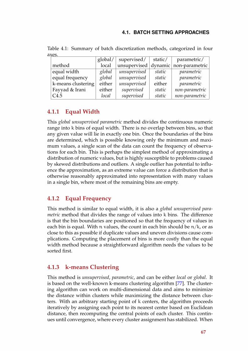
4.1. BATCH SETTING APPROACHES
Table 4.1: Summary of batch discretization methods, categorized in fouraxes.
global/ supervised/ static/ parametric/method local unsupervised dynamic non-parametricequal width global unsupervised static parametricequal frequency global unsupervised static parametrick-means clustering either unsupervised either parametricFayyad & Irani either supervised static non-parametricC4.5 local supervised static non-parametric
4.1.1 Equal Width
This global unsupervised parametric method divides the continuous numericrange into k bins of equal width. There is no overlap between bins, so thatany given value will lie in exactly one bin. Once the boundaries of the binsare determined, which is possible knowing only the minimum and maxi-mum values, a single scan of the data can count the frequency of observa-tions for each bin. This is perhaps the simplest method of approximating adistribution of numeric values, but is highly susceptible to problems causedby skewed distributions and outliers. A single outlier has potential to influ-ence the approximation, as an extreme value can force a distribution that isotherwise reasonably approximated into representation with many valuesin a single bin, where most of the remaining bins are empty.
4.1.2 Equal Frequency
This method is similar to equal width, it is also a global unsupervised para-metric method that divides the range of values into k bins. The differenceis that the bin boundaries are positioned so that the frequency of values ineach bin is equal. With n values, the count in each bin should be n/k, or asclose to this as possible if duplicate values and uneven divisions cause com-plications. Computing the placement of bins is more costly than the equalwidth method because a straightforward algorithm needs the values to besorted first.
4.1.3 k-means Clustering
This method is unsupervised, parametric, and can be either local or global. Itis based on the well-known k-means clustering algorithm [77]. The cluster-ing algorithm can work on multi-dimensional data and aims to minimizethe distance within clusters while maximizing the distance between clus-ters. With an arbitrary starting point of k centers, the algorithm proceedsiteratively by assigning each point to its nearest center based on Euclideandistance, then recomputing the central points of each cluster. This contin-ues until convergence, where every cluster assignment has stabilized. When
67

CHAPTER 4. NUMERIC ATTRIBUTES
used for static discretization the clustering will be performed on a single at-tribute at a time. Dynamic discretization is possible by clustering severalattributes simultaneously.
4.1.4 Fayyad and Irani
This method [45] is quite different from those described above as it is super-vised and non-parametric. The algorithm is categorized [41] as capable of bothglobal and local operation. The values of an attribute are first sorted, then acut-point between every adjacent pair of values is evaluated, with n valuesand no repeated values this involves n − 1 evaluations. The counts of classlabels to either side of each split candidate determine the information gain inthe same way that attributes are chosen during tree induction (Section 3.1).The information gain has been found to be a good heuristic for dividingvalues while taking class labels into consideration. The cut-point with thehighest gain is used to divide the range into two sets, and the procedurecontinues by recursively cutting both sets. Fayyad and Irani show [45] thatthis procedure will never choose a cut-point between consecutive examplesof the same class, leading to an optimization of the algorithm that avoidsevaluation of such points.
A stopping criterion is necessary to avoid dividing the range too finely,failure to terminate the algorithm could potentially continue division untilthere is a unique interval per value. If an interval is pure, that is, has valuesall of the same class, then there is no reason to continue splitting. If an inter-val has a mixture of labels, Fayyad and Irani apply the principle of minimumdescription length (MDL) [133] to estimate when dividing the numeric rangeceases to provide any benefit.
4.1.5 C4.5
The procedure for discretizing numeric values in Quinlan’s C4.5 [131] de-cision tree learner is local, supervised and non-parametric. It essentially usesthe same procedure described in Fayyad and Irani’s method, only it is notrecursively applied in the same manner. For the purposes of inducing adecision tree, a single two-way split is chosen and evaluated for every nu-meric attribute. The cut-points are decided locally on the respective subsetof every node, in the same way as described above—scanning through thevalues in order and calculating the information gain of candidate cut-pointsto determine the point with the highest gain. The difference is that the scanis carried out only once per numeric attribute to find a single split into twosubsets, and no further recursion is performed on those subsets at that point.The recursive nature of decision tree induction means however that numericranges can be cut again further down the tree, but it all depends on whichattributes are selected during tree growth. Splits on different attributes willaffect the subsets of examples that are subsequently evaluated.
Responding to results in [41] showing that global pre-discretization of
68

4.2. DATA STREAM APPROACHES
data using Fayyad and Irani’s method could produce better C4.5 trees thanusing C4.5’s local method, Quinlan improved the method in C4.5 release8 [132] by removing some bias in the way that numeric cut-points were cho-sen.
4.2 Data Stream Approaches
The first thing to consider are ways in which the batch methods from theprevious section could be applied to the data stream setting.
The equal width method is simple to perform in a single pass and lim-ited memory provided that the range of values is known in advance. Thisrequirement could easily violate the requirements of a data stream scenariobecause unless domain knowledge is provided by the user the only wayto determine the true range is to do an initial pass of the data, turning thesolution into a two-pass operation. This text only considers solutions thatwork in a single pass. Conceivably an adaptive single-pass version of thealgorithm could be used, such as described by Gama and Pinto [61], whereany values outside of the known range would trigger a reorganization ofthe bins. However, even if a single-pass solution were available, it wouldstill be prone to the problem of outliers.
Equal frequency appears more difficult to apply to data streams thanequal width because the most straightforward implementation requires thedata to be sorted. The field of database optimization has studied meth-ods for constructing equal frequency intervals, or equivalently equi-depthhistograms or computation of quantiles, from a single pass. The literaturerelated to this is surveyed in Section 4.2.3.
A method similar to k-means discretization for data streams would re-quire a clustering algorithm that is capable of working on a stream. Datastream clustering is outside the scope of this text, but the problem has beenworked on by several researchers such as Guha et al. [70, 69].
Fayyad and Irani’s discretization algorithm and the similar method builtinto C4.5 require the data to be sorted in order to search for the best cut-point.
A rare example of a discretization method specifically intended to op-erate on data streams for machine learning purposes is presented by Gamaand Pinto [61]. It works by maintaining two layers—the first layer simpli-fies the data with an equal width summary that is incrementally updatedand the second layer builds the final histogram, either equal width or equalfrequency, and is only updated as needed.
Methods that are global are applied as a separate pre-processing step be-fore learning begins, while local methods are integrated into a learning algo-rithm, where discretization happens during learning as needed. Since onlysingle-pass solutions to learning are considered, straightforward implemen-tation of global discretization is not viable, as this would require an initialpass to discretize the data, to be followed by a second pass for learning. Un-
69

CHAPTER 4. NUMERIC ATTRIBUTES
fortunately this discounts direct application of all global solutions looked atthus far, leaving few options apart from C4.5. The attractive flexibility af-forded in the batch setting by separating discretization as a pre-processingstep does not transfer to the demands of the data stream setting.
For Hoeffding tree induction the discretization can be integrated withlearning by performing local discretization on the subsets of data found atactive leaves, those in search of splits. The number of examples that con-tribute to growth decisions at any one time are limited, depending on thetotal number of active leaves in the tree. A brute-force approach stores everyexample in a leaf until a split decision is made. Without memory manage-ment the number of active leaves in the tree can grow without bound, mak-ing it impossible to use brute force without a suitable memory managementscheme.
The methods discussed in the following subsections represent variousproposals from the literature for handling numeric values during Hoeffd-ing tree induction. At a higher level they are all trying to reproduce theC4.5 discretization method in the stream setting, so in this sense they are allsupervised methods. The difference between them is that they approximatethe C4.5 process in different ways. The exhaustive binary tree approach (Sec-tion 4.2.2) represents the brute-force approach of remembering all values,thus is a recreation of the batch technique. Awareness of space-efficiency asa critical concern in processing data streams has led to other methods ap-plying a two-stage approach. Discretization methods at the first stage areused to reduce space costs, intended to capture the sorted distribution ofclass label frequencies. These are then used as input for the second stage,which makes a supervised C4.5-style two-way split decision.
In addition to the distinctions introduced earlier, a final dimension is in-troduced to help distinguish between the methods: all-class vs per-class. Theall-class methods produce a single approximation of the distribution of ex-amples, such as a single set of boundaries, recording the frequency of allclasses over one approximation. In contrast, the per-class methods producea different approximation per class, so for example each class is representedby an independent set of boundaries. The per-class methods are supervisedin the sense that the class labels influence the amount of attention given tocertain details—by allocating the same amount of space to the approxima-tion of each class the per-class methods studied here enforce equal attentionto each class.
The discretization methods for Hoeffding trees are discussed next, withproperties summarized in Table 4.2.
4.2.1 VFML Implementation
Although Domingos and Hulten have not published any literature describ-ing a method for handling numeric attributes, they have released workingsource code in the form of their VFML package [88]. VFML is written in Cand includes an implementation of VFDT that is capable of learning from
70

4.2. DATA STREAM APPROACHES
Table 4.2: Summary of stream discretization methods. All methods are local,static, and involve two stages, the second of which is supervised.
per-class all-classparametric quantile summaries VFML
Gaussian approx. (2nd stage)non-parametric Gaussian approx. (1st stage) exhaustive binary tree
streams with numeric attributes.This method is all-class and parametric, although the original implemen-
tation hides the single parameter. Numeric attribute values are summarizedby a set of ordered bins, creating a histogram. The range of values coveredby each bin is fixed at creation and does not change as more examples areseen. The hidden parameter is a limit on the total number of bins allowed—in the VFML implementation this is hard-coded to allow a maximum of onethousand bins. Initially, for every new unique numeric value seen, a newbin is created. Once the fixed number of bins have been allocated, eachsubsequent value in the stream updates the counter of the nearest bin.
There are two potential issues with the approach. The first is that themethod is sensitive to data order. If the first one thousand examples seenin a stream happen to be skewed to one side of the total range of values,then the final summary will be incapable of accurately representing the fullrange of values.
The other issue is estimating the optimal number of bins. Too few binswill mean the summary is small but inaccurate, and many bins will increaseaccuracy at the cost of space. In the experimental comparison the maximumnumber of bins is varied to test this effect.
4.2.2 Exhaustive Binary Tree
This method represents the case of achieving perfect accuracy at the neces-sary expense of storage space. It is non-parametric and all-class. The decisionsmade are the same that a batch method would make, because essentially it isa batch method—no information is discarded other than the observed orderof values.
Gama et al. present this method in their VFDTc system [62]. It works byincrementally constructing a binary tree structure as values are observed.The path a value follows down the tree depends on whether it is less than,equal to or greater than the value at a particular node in the tree. The valuesare implicitly sorted as the tree is constructed.
This structure saves space over remembering every value observed at aleaf when a value that has already been recorded reappears in the stream. Inmost cases a new node will be introduced to the tree. If a value is repeatedthe counter in the binary tree node responsible for tracking that value canbe incremented. Even then, the overhead of the tree structure will mean thatspace can only be saved if there are many repeated values. If the number of
71
CHAPTER 4. NUMERIC ATTRIBUTES
unique values were limited, as is the case in some data sets, then the storagerequirements will be less intensive. In all of the synthetic data sets used forthis study the numeric values are generated randomly across a continuousrange, so the chance of repeated values is almost zero.
The primary function of the tree structure is to save time. It lowers thecomputational cost of remembering every value seen, but does little to re-duce the space complexity. The computational considerations are impor-tant, because a slow learner can be even less desirable than one that con-sumes a large amount of memory.
Beside memory cost, this method has other potential issues. Becauseevery value is remembered, every possible threshold is also tested whenthe information gain of split points is evaluated. This makes the evaluationprocess more costly than more approximate methods.
This method is also prone to data order issues. The layout of the tree isestablished as the values arrive, such that the value at the root of the treewill be the first value seen. There is no attempt to balance the tree, so dataorder is able to affect the efficiency of the tree. In the worst case, an orderedsequence of values will cause the binary tree algorithm to construct a list,which will lose all the computational benefits compared to a well balancedbinary tree.
4.2.3 Quantile Summaries
The field of database research is also concerned with the problem of sum-marizing the numeric distribution of a large data set in a single pass andlimited space. The ability to do so can help to optimize queries over mas-sive databases [140].
Researchers in the field of database research are concerned with accu-racy guarantees associated with quantile estimates, helping to improve thequality of query optimizations. Random sampling is often considered as asolution to this problem. Vitter [152] shows how to randomly sample from adata stream, but the non-deterministic nature of random sampling and thelack of accuracy guarantees motivate search for other solutions. Munro andPaterson [121] show how an exact quantile can be deterministically com-puted from a single scan of the data, but that this requires memory propor-tional to the number of elements in the data. Using less memory meansthat quantiles must be approximated. Early work in quantile approxima-tion includes the P2 algorithm proposed by Jain and Chlamtac [92], whichtracks five markers and updates them as values are observed via piecewisefitting to a parabolic curve. The method does not provide guarantees on theaccuracy of the estimates. Agrawal and Swami [3] propose a method thatadaptively adjusts the boundaries of a histogram, but it too fails to providestrong accuracy guarantees. More recently, the method of Alsabti et al. [5]provides guaranteed error bounds, continued by Manku et al. [112] whodemonstrate an improved method with tighter bounds.
The quantile estimation algorithm of Manku et al. [112] was the best
72
4.2. DATA STREAM APPROACHES
known method until Greenwald and Khanna [67] proposed a quantile sum-mary method with even stronger accuracy guarantees, thus representing thebest current known solution. The method works by maintaining an orderedset of tuples, each of which records a value from the input stream, alongwith implicit bounds for the range of each value’s true rank. An operationfor compressing the quantile summary is defined, guaranteeing that the er-ror of the summary is kept within a desired bound. The quantile summary issaid to be ε-approximate, after seeingN elements of a sequence any quantileestimate returned will not differ from the exact value by more than εN. Theworst-case space requirement is shown by the authors to be O( 1
εlog(εN)),
with empirical evidence showing it to be even better than this in practice.Greenwald and Khanna mention two variants of the algorithm. The
adaptive variant is the basic form of the algorithm, that allocates more spaceonly as error is about to exceed the desired ε. The other form, used by thistext, is referred to as the pre-allocated variant, which imposes a fixed limiton the amount of memory used. Both variants are parametric—for adap-tive the parameter is ε, for pre-allocated the parameter is a tuple limit. Thepre-allocated method was chosen because it guarantees stable approximationsizes throughout the tree, and is consistent with the majority of other meth-ods by placing upper bounds on the memory used per leaf.
When used to select numeric split points in Hoeffding trees, a per-classapproach is used where a separate quantile summary is maintained perclass label. When evaluating split decisions, all values stored in the tuplesare tested as potential split points.
4.2.4 Gaussian Approximation
This method approximates a numeric distribution on a per-class basis insmall constant space, using a Gaussian (commonly known as normal) dis-tribution. Such a distribution can be incrementally maintained by storingonly three numbers in memory, and is completely insensitive to data order.A Gaussian distribution is essentially defined by its mean value, which isthe center of the distribution, and standard deviation or variance, whichis the spread of the distribution. The shape of the distribution is a classicbell-shaped curve that is known by scientists and statisticians to be a goodrepresentation of certain types of natural phenomena, such as the weightdistribution of a population of organisms.
Algorithm 3 describes a method for incrementally computing the meanand variance of a stream of values. It is a method that can be derived fromstandard statistics textbooks. The method only requires three numbers tobe remembered, but is susceptible to rounding errors that are a well-knownlimitation of computer number representation.
A more robust method that is less prone to numerical error is given as Al-gorithm 4. It also requires only three values in memory, but maintains themin a way that is less vulnerable to rounding error. This method was derivedfrom the work of Welford [156], and its advantages are studied in [28]. This
73

CHAPTER 4. NUMERIC ATTRIBUTES
Algorithm 3 Textbook incremental Gaussian.weightSum = 0
valueSum = 0
valueSqSum = 0
for all data points (value, weight) doweightSum = weightSum+weight
valueSum = valueSum+ value×weightvalueSqSum = valueSqSum+ value× value×weight
end for
anytime output:return mean = valuesSum
weightSum
return variance = valueSqSum−mean×valueSumweightSum−1
is the method used in the experimental implementation.
Algorithm 4 Numerically robust incremental Gaussian.weightSum = weightfirstmean = valuefirstvarianceSum = 0
for all data points (value, weight) after first doweightSum = weightSum+weight
lastMean = mean
mean = mean+ value−lastMeanweightSum
varianceSum = varianceSum+(value−lastMean)×(value−mean)
end for
anytime output:return mean = mean
return variance = varianceSumweightSum−1
For each numeric attribute the numeric approximation procedure main-tains a separate Gaussian distribution per class label. A method similarto this is described by Gama et al. in their UFFT system [60]. To handlemore than two classes, the system builds a forest of trees, one tree for eachpossible pair of classes. When evaluating split points in that case, a sin-gle optimal point is computed as derived from the crossover point of twodistributions. It is possible to extend the approach, however, to search forsplit points, allowing any number of classes to be handled by a single tree.The possible values are reduced to a set of points spread equally across therange, between the minimum and maximum values observed. The numberof evaluation points is determined by a parameter, so the search for splitpoints is parametric, even though the underlying Gaussian approximationsare not. For each candidate point the weight of values to either side of the
74

4.2. DATA STREAM APPROACHES
Figure 4.1: Gaussian approximation of 2 classes.
split can be approximated for each class, using their respective Gaussiancurves, and the information gain is computed from these weights.
The process is illustrated in Figures 4.1-4.3. At the top of each figure areGaussian curves, each curve approximates the distribution of values seenfor a numeric attribute and labeled with a particular class. The curves canbe described using three values; the mean value, the standard deviationor variance of values, and the total weight of examples. For example, inFigure 4.1 the class shown to the left has a lower mean, higher variance andhigher example weight (larger area under the curve) than the other class.Below the curves the range of values has been divided into ten split points,labeled A to J. The horizontal bars show the proportion of values that areestimated to lie on either side of each split, and the vertical bar at the bottomdisplays the relative amount of information gain calculated for each split.For the two-class example (Figure 4.1), the split point that would be chosenas the best is point E, which according to the evaluation has the highestinformation gain. In the three-class example (Figure 4.2) the preferred splitpoint is point D. In the four-class example (Figure 4.3) the split point C ischosen which nicely separates the first class from the others.
A refinement to this method, found to increase precision at low addi-tional cost in early experiments, is used in the final implementation. It in-volves also tracking the minimum and maximum values of each class. Thisrequires storing an extra two counts per class, but precisely maintainingthese values is simple and fast. When evaluating split points the per-classminimum and maximum information is exploited to determine when classvalues lie completely to one side of a split, eliminating the small uncertaintyotherwise present in the tails of the Gaussian curves. From the per-class
75

CHAPTER 4. NUMERIC ATTRIBUTES
Figure 4.2: Gaussian approximation of 3 classes.
Figure 4.3: Gaussian approximation of 4 classes.
76

4.2. DATA STREAM APPROACHES
minimum and maximum, the minimum and maximum of the entire rangeof values can be established, which helps to determine the position of splitpoints to evaluate.
Intuitively it may seem that split points will only occur between the low-est and highest class mean, but this is not true. Consider searching for asplit on the age attribute of the GENF1 data stream. The function is definedon page 36, where the first class has age values that are less than 40 andgreater than 60, and the second class has age values between 40 and 60.Obviously either 40 or 60 are the optimal split points, but the means of bothclass distributions will lie somewhere between 40 and 60—the first class willhave a large variance estimate, and the second will be much narrower. Thismotivates searching across the entire range of values for a split. Using theabsolute minimum and maximum value makes the procedure susceptibleto outliers similar to the weakness of equal width discretization. A morerobust search may instead consider each mean plus or minus several stan-dard deviations to determine the potential splitting range. This possibilityis reserved for future work.
Simple Gaussian approximation will almost certainly not capture the fulldetail of an intricate numeric distribution, but is highly efficient in bothcomputation and memory. Where the binary tree method uses extremememory costs to be as accurate as possible, this method employs the oppo-site approach—using gross approximation to use as little memory as possi-ble.
This simplified view of numeric distributions is not necessarily harmfulto the accuracy of the trees it produces. There will be further opportuni-ties to refine split decisions on a particular attribute by splitting again fur-ther down the tree. All methods have multiple attempts at finding values,where each subsequent attempt will be in a more focused range of valuesthus based on increasingly confident information. The more approximateGaussian method relies on this more than the less approximate approaches.Also, the Gaussian approximation may prove more robust and resistant tonoisy values than more complicated methods, which concentrate on finerdetails.
4.2.5 Numerical Interval Pruning
Another contribution is the work of Jin and Agrawal [93] who present anapproach called numerical interval pruning (NIP). The authors claim it is anefficient method “which significantly reduces the processing time for nu-merical attributes, without loss in accuracy.” Unfortunately insufficient de-tails for reproducing the technique are provided in the paper. The numericattribute range is divided into equal width intervals, and the intervals arethen pruned if statistical tests determine that they are not likely to containthe best split point. Information is maintained in three ways—small classhistograms, concise class histograms and detailed information (which canbe in one of two formats, depending on which is most efficient). Without
77

CHAPTER 4. NUMERIC ATTRIBUTES
access to an actual implementation of their approach it is hard to be surethat any attempted reproduction of the technique, based on informationprovided in their paper, will be sufficiently faithful to the original. In theirexperimental evaluation, they found that the NIP method had more impacton computational cost than memory, in which they saw an average 39% re-duction in runtime compared to an exhaustive search for split points. Basedon these findings, it should be possible to relate NIP performance to that ofthe binary tree. Judging by the reports, both methods are highly accurate,but in terms of memory NIP would be more efficient than the binary tree bya small amount. The experimental results show that even if a method is sev-eral times more space efficient than the exhaustive method it is still unlikelyto compete with methods that use small and constant space per node.
78

5Prediction Strategies
The previous chapters have considered the induction of Hoeffding trees.Chapter 3 covered the basic induction of Hoeffding trees, followed by Chap-ter 4 which investigated the handling of continuous numeric attributes inthe training data. This chapter focuses on the use of models once they havebeen induced—how predictions are made by the trees. Section 5.1 describesthe standard majority class prediction method. Attempts to outperform thismethod are described in Section 5.2 and 5.3.
5.1 Majority Class
Prediction using decision trees is straightforward. Examples with unknownlabel are filtered down the tree to a leaf, and the most likely class label re-trieved from the leaf. An obvious and straightforward way of assigning la-bels to leaves is to determine the most frequent class of examples that wereobserved there during training. This method is used by the batch methodsC4.5/CART and is naturally replicated in the stream setting by Hoeffdingtrees. If the likelihood of all class labels is desired, an immediate extensionis to return a probability distribution of class labels, once again based on thedistribution of classes observed from the training examples.
Table 5.1 is used to illustrate different prediction schemes throughout thechapter. In the case of majority class, the leaf will always predict class C2 forevery example, because most examples seen before have been of that class.There have been 60 examples of class C2 versus 40 examples of class C1, sothe leaf will estimate for examples with unknown class that the probabilityof class C2 is 0.6, and the probability of C1 is 0.4.
5.2 Naive Bayes Leaves
There is more information available during prediction in the leaves of a Ho-effding tree than is considered using majority class classification. The at-tribute values determine the path of each example down the tree, but oncethe appropriate leaf has been established it is possible to use the same at-tribute values to further refine the classification. Gama et al. call this en-hancement functional tree leaves [60, 62].
79

CHAPTER 5. PREDICTION STRATEGIES
Table 5.1: Example sufficient statistics in a leaf after 100 examples have beenseen. There are two class labels: C1 has been seen 40 times, and C2 has beenseen 60 times. There are three attributes: A1 can either have value A or B,A2 can be C, D or E, and A3 can be F, G, H or I. The values in the table trackhow many times each of the values have been seen for each class label.
A1 A2 A3A B C D E F G H I class total12 28 5 10 25 13 9 3 15 C1 4034 26 21 8 31 11 21 19 9 C2 60
If P(C) is the probability of event C occurring, and P(C|X) is the proba-bility of event C given that X occurs, then from Bayes’ theorem:
P(C|X) =P(X|C)P(C)
P(X)(5.1)
This rule is the foundation of the Naive Bayes classifier [107]. The classi-fier is called ‘naive’ because it assumes independence of the attributes. Theindependence assumption means that for each example the value of anyattribute will not have a bearing on the value of any other attribute. It isnot realistic to expect such simplistic attribute relationships to be commonin practice, but despite this the classifier works surprisingly well in gen-eral [40, 81].
By collecting the probabilities of each attribute value with respect to theclass label from training examples, the probability of the class for unlabeledexamples can be computed. Fortunately, the sufficient statistics being main-tained in leaves of a Hoeffding tree for the purpose of choosing split testsare also the statistics required to perform Naive Bayes classification.
Returning to the example in Table 5.1, if an example being classified bythe leaf has attribute values A1=B, A2=E and A3=I then the likelihood of theclass labels is calculated using Equation 5.1:
P(C1|X) =P(X|C1)P(C1)
P(X)
=[P(B|C1)× P(E|C1)× P(I|C1)]× P(C1)
P(X)
=2840× 25
40× 15
40× 40
100
P(X)
=0.065625
P(X)
80
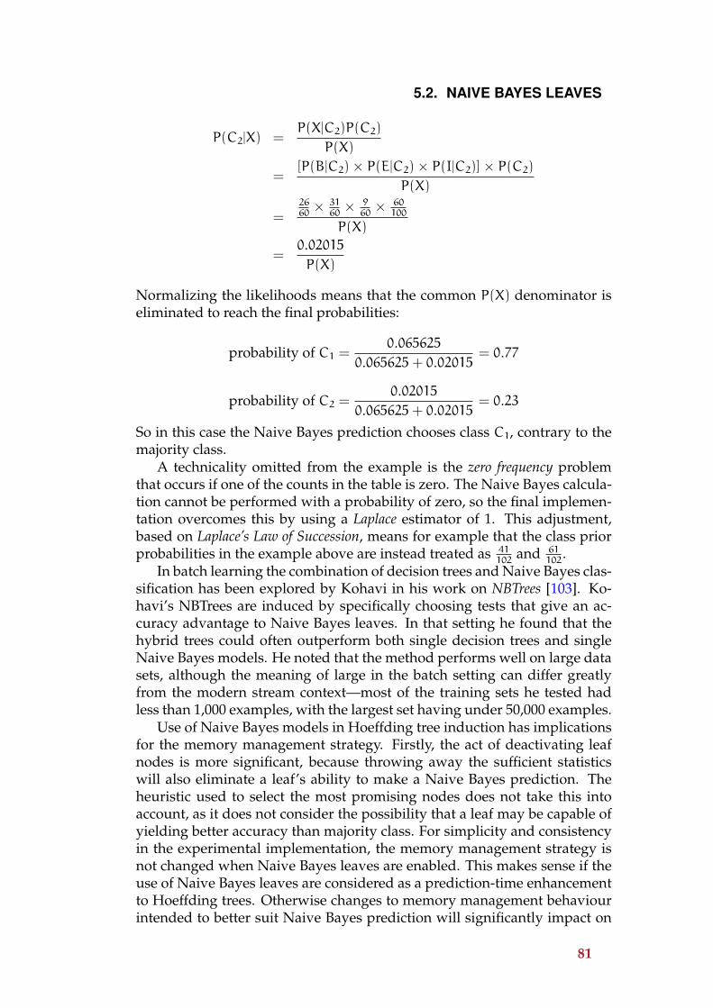
5.2. NAIVE BAYES LEAVES
P(C2|X) =P(X|C2)P(C2)
P(X)
=[P(B|C2)× P(E|C2)× P(I|C2)]× P(C2)
P(X)
=2660× 31
60× 9
60× 60
100
P(X)
=0.02015
P(X)
Normalizing the likelihoods means that the common P(X) denominator iseliminated to reach the final probabilities:
probability of C1 =0.065625
0.065625+ 0.02015= 0.77
probability of C2 =0.02015
0.065625+ 0.02015= 0.23
So in this case the Naive Bayes prediction chooses class C1, contrary to themajority class.
A technicality omitted from the example is the zero frequency problemthat occurs if one of the counts in the table is zero. The Naive Bayes calcula-tion cannot be performed with a probability of zero, so the final implemen-tation overcomes this by using a Laplace estimator of 1. This adjustment,based on Laplace’s Law of Succession, means for example that the class priorprobabilities in the example above are instead treated as 41
102and 61
102.
In batch learning the combination of decision trees and Naive Bayes clas-sification has been explored by Kohavi in his work on NBTrees [103]. Ko-havi’s NBTrees are induced by specifically choosing tests that give an ac-curacy advantage to Naive Bayes leaves. In that setting he found that thehybrid trees could often outperform both single decision trees and singleNaive Bayes models. He noted that the method performs well on large datasets, although the meaning of large in the batch setting can differ greatlyfrom the modern stream context—most of the training sets he tested hadless than 1,000 examples, with the largest set having under 50,000 examples.
Use of Naive Bayes models in Hoeffding tree induction has implicationsfor the memory management strategy. Firstly, the act of deactivating leafnodes is more significant, because throwing away the sufficient statisticswill also eliminate a leaf’s ability to make a Naive Bayes prediction. Theheuristic used to select the most promising nodes does not take this intoaccount, as it does not consider the possibility that a leaf may be capable ofyielding better accuracy than majority class. For simplicity and consistencyin the experimental implementation, the memory management strategy isnot changed when Naive Bayes leaves are enabled. This makes sense if theuse of Naive Bayes leaves are considered as a prediction-time enhancementto Hoeffding trees. Otherwise changes to memory management behaviourintended to better suit Naive Bayes prediction will significantly impact on
81

CHAPTER 5. PREDICTION STRATEGIES
overall tree induction, making it harder to interpret direct comparisons withmajority class trees.
The outcome of this approach is that when memory gets tight and fewerof the leaves are allowed to remain active, then fewer of the leaves will becapable of Naive Bayes prediction. The fewer the active leaves, the closerthe tree will behave to a tree that uses majority class only. By the time thetree is frozen and can no longer afford to hold any active leaves in memorythen the tree will have completely reverted to majority class prediction. Thisbehaviour is noted when looking at the experimental results.
The other issue is the secondary memory management strategy of re-moving poor attributes (Section 3.3.1). This too will alter the effectivenessof Naive Bayes models, because removing information about attributes re-moves some of the power that the Naive Bayes models use to predict, re-gardless of whether the attributes are deemed a poor candidate for splittingor not. As the removal strategy has been shown to not have a large bear-ing on final tree accuracy, whenever Naive Bayes leaves are employed theattribute removal strategy is not used.
Memory management issues aside, the Naive Bayes enhancement addsno cost to the induction of a Hoeffding tree, neither to the training speed normemory usage. All of the extra work is done at prediction time. The amountof prediction-time overhead is quantified in the experimental comparison.
Early experimental work confirmed that Naive Bayes predictions are ca-pable of increasing accuracy as Gama et al. observed [60, 62], but also ex-posed cases where Naive Bayes prediction fares worse than majority class.The first response to this problem was to suspect that some of the leaf mod-els are immature. In the early stages of a leaf’s development the probabili-ties estimated may be unreliable because they are based on very few obser-vations. If that is the case then there are two possible remedies; either (1)give them a jump-start to make them more reliable from the beginning, or(2) wait until the models are more reliable before using them.
Previous work [83] has covered several attempts at option (1) of ‘prim-ing’ new leaves with better information. One such attempt, suggested byGama et al. [60] is to remember a limited number of the most recent exam-ples from the stream, for the purposes of training new leaves as soon as theyare created. A problem with this idea is that the number of examples able tobe retrieved that apply to a particular leaf will diminish as the tree gets pro-gressively deeper. Other attempts at priming involved trying to inject moreof the information known prior to splitting into the resulting leaves of thesplit. Neither of these attempts were successful at overcoming the problemso are omitted from consideration.
5.3 Adaptive Hybrid
Cases where Naive Bayes decisions are less accurate than majority class area concern because more effort is being put in to improve predictions and
82

5.3. ADAPTIVE HYBRID
instead the opposite occurs. In those cases it is better to use the standardmajority class method, making it harder to recommend the use of NaiveBayes leaf predictions in all situations.
The method described here tries to make the use of Naive Bayes mod-els more reliable, by only trusting them on a per-leaf basis when there isevidence that there is a true gain to be made. The adaptive method worksby monitoring the error rate of majority class and Naive Bayes decisions inevery leaf, and choosing to employ Naive Bayes decisions only where theyhave been more accurate in past cases. Unlike pure Naive Bayes prediction,this process does introduce an overhead during training. Extra time is spentper training example generating both prediction types and updating errorestimates, and extra space per leaf is required for storing the estimates.
Algorithm 5 Adaptive prediction algorithm.for all training examples do
Sort example into leaf l using HTifmajorityClassl 6= true class of example then
incrementmcErrorlend ifif NaiveBayesPredictionl(example) 6= true class of example then
increment nbErrorlend ifUpdate sufficient statistics in l...
end for
for all examples requiring label prediction doSort example into leaf l using HTif nbErrorl < mcErrorl then
return NaiveBayesPredictionl(example)else
return majorityClasslend if
end for
The pseudo-code listed in Algorithm 5 makes the process explicit. Dur-ing training, once an example is filtered to a leaf but before the leaf is up-dated, both majority class prediction and Naive Bayes prediction are per-formed and both are compared with the true class of the example. Countersare incremented in the leaf to reflect how many errors the respective meth-ods have made. At prediction time, a leaf will use majority class predictionunless the counters suggest that Naive Bayes prediction has made fewererrors, in which case Naive Bayes prediction is used instead.
In terms of the example in Table 5.1, the class predicted for new exampleswill depend on extra information. If previous training examples were moreaccurately classified by majority class than Naive Bayes then classC2 will be
83

CHAPTER 5. PREDICTION STRATEGIES
returned, otherwise the attribute values will aid in Naive Bayes predictionas described in the previous subsection.
84

6Hoeffding Tree Ensembles
In machine learning classification, an ensemble of classifiers is a collection ofseveral models combined together. Algorithm 6 lists a generic procedurefor creating ensembles that is commonly used in batch learning.
Algorithm 6 Generic ensemble training algorithm.1: Given a set of training examples S2: for all models hm in the ensemble ofMmodels,m ∈ {1, 2, ...,M} do3: Assign a weight to each example in S to create weight distributionDm
4: Call base learner, providing it with Smodified by weight distributionDm to create hypothesis hm
5: end for
This procedure requires three elements to create an ensemble:
1. A set S of training examples
2. A base learning algorithm
3. A method of assigning weights to examples (line 3 of the pseudo-code)
The third requirement, the weighting of examples, forms the major dif-ference between ensemble methods. Another potential difference is the vot-ing procedure. Typically each member of the ensemble votes towards theprediction of class labels, where voting is either weighted or unweighted. Inweighted voting individual classifiers have varying influence on the finalcombined vote, the models that are believed to be more accurate will betrusted more than those that are less accurate on average. In unweightedvoting all models have equal weight, and the final predicted class is thelabel chosen by the majority of ensemble members. Ensemble algorithms,algorithms responsible for inducing an ensemble of models, are sometimesknown as meta-learning schemes. They perform a higher level of learningthat relies on lower-level base methods to produce the individual models.
Ensemble methods are attractive because they can often be more accu-rate than a single classifier alone. The best ensemble methods are modu-lar, capable of taking any base algorithm and improving its performance—any method can be taken off the shelf and ‘plugged in’. Besides the added
85

CHAPTER 6. HOEFFDING TREE ENSEMBLES
memory and computational cost of sustaining multiple models, the maindrawback is loss of interpretability. A single decision tree may be easily in-terpreted by humans, whereas the combined vote of several trees will bedifficult to interpret.
In batch learning, cases where the base model is already difficult to in-terpret or a black-box solution is acceptable, the potential for improved accu-racy easily justifies the use of ensembles where possible. In the data streamsetting, the memory and time requirements of multiple models need moreserious consideration. The demands of a data stream application will besensitive to the additive effect of introducing more models, and there willbe limits to the numbers of models that can be supported. In limited mem-ory learning—which is better, a single large model or many smaller modelsof equivalent combined size?
An ensemble of classifiers will be more accurate than any of its individ-ual members if two conditions are met [75, 148]. Firstly, the models mustbe accurate, that is, they must do better than random guessing. Secondly,they must be diverse, that is, their errors should not be correlated. If theseconditions are satisfied Hansen and Salamon [75] show that as the numberof ensemble members increase, the error of the ensemble will tend towardszero in the limit. The accuracy of an ensemble in practice will fall short ofthe improvement that is theoretically possible, mostly because the memberswhich have been trained on variations of the same training data will neverbe completely independent.
Dietterich surveys ensemble methods for machine learning classifica-tion [35]. He mentions three possible reasons for the success of ensemblemethods in practice: statistical, computational and representational. Thestatistical contribution to success is that the risk of incorrect classificationis shared among multiple members, so that the average risk is lower thanrelying on a single member alone. The computational contribution is thatmore than one attempt is made to learn what could be a computationally in-tractable problem, where each attempt guided by heuristics could get stuckin local minima, but the average of several different attempts could bettersolve the problem than any individual attempt. The representational contri-bution is that an ensemble of models may be more capable of representingthe true function in the data than any single model in isolation.
Decision trees are the basic machine learning model being investigatedby this text, and they make an excellent base for ensemble methods, forseveral reasons given below. This is verified in practice, where ensembles ofdecision trees are ranked among the best known methods in contemporarymachine learning [27].
The statistical reasoning and the uncorrelated errors theories both sug-gest that member diversity is crucial to good ensemble performance. En-semble methods typically exploit the lack of stability of a base learner toincrease diversity, thus achieve the desired effect of better accuracy in com-bination. Breiman [17] defines stable methods as those not sensitive to smallchanges in training data—the more sensitive a method is to data changes the
86

0
20
40
60
80
100
2 4 6 8 10 12 14
num
ber
of le
aves
memory size
1 tree2 trees3 trees4 trees5 trees
Figure 6.1: A simple model of the leaf count of combinations of decisiontrees as a function of total memory size.
more unstable it is said to be. Decision trees are good candidates for ensem-bles because they are inherently unstable. The greedy local decisions caneasily be influenced by only slight differences in training data, and the ef-fect of a single change will be propagated to the entire subtree below. NaiveBayes in contrast is stable as it takes substantial differences in training datato modify its outcome.
In the stream setting, the nature of the Hoeffding bound decision mightsuggest that Hoeffding trees may not exhibit such instability. However,the bound only guides local per-split decisions—Domingos and Hulten [39]prove that overall the algorithm approximates the batch induction of deci-sion trees. The empirical results of the tree ensembles in the next chapterdemonstrate that Hoeffding trees are indeed unstable.
Decision trees also suit the computational argument. Computing an op-timal decision tree is an NP-complete problem [89], so out of necessity thealgorithm performs a greedy local search. Several decision trees can ap-proach the problem based on different searches involving local greedy deci-sions, which on average may form a better approximation of the true targetthan any single search.
It is interesting to consider the representational argument applied to en-sembles of decision trees, especially where memory is limited. In theoryan ensemble of decision trees can be represented by a single standard deci-sion tree, but the cost of constructing such a tree is expensive. Consider theprocess of combining two trees, A and B. This can be achieved by replac-ing every leaf of A with a subtree that is a complete copy of tree B, where
87
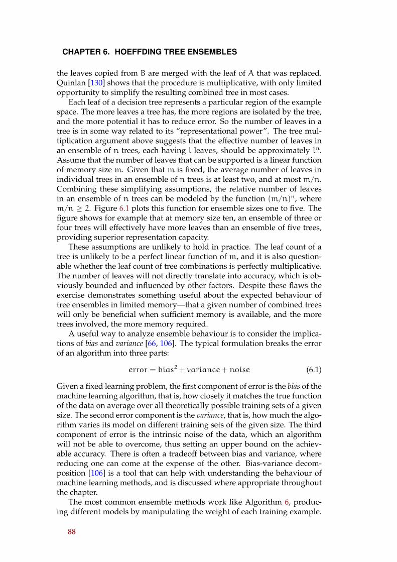
CHAPTER 6. HOEFFDING TREE ENSEMBLES
the leaves copied from B are merged with the leaf of A that was replaced.Quinlan [130] shows that the procedure is multiplicative, with only limitedopportunity to simplify the resulting combined tree in most cases.
Each leaf of a decision tree represents a particular region of the examplespace. The more leaves a tree has, the more regions are isolated by the tree,and the more potential it has to reduce error. So the number of leaves in atree is in some way related to its “representational power”. The tree mul-tiplication argument above suggests that the effective number of leaves inan ensemble of n trees, each having l leaves, should be approximately ln.Assume that the number of leaves that can be supported is a linear functionof memory size m. Given that m is fixed, the average number of leaves inindividual trees in an ensemble of n trees is at least two, and at most m/n.Combining these simplifying assumptions, the relative number of leavesin an ensemble of n trees can be modeled by the function (m/n)n, wherem/n ≥ 2. Figure 6.1 plots this function for ensemble sizes one to five. Thefigure shows for example that at memory size ten, an ensemble of three orfour trees will effectively have more leaves than an ensemble of five trees,providing superior representation capacity.
These assumptions are unlikely to hold in practice. The leaf count of atree is unlikely to be a perfect linear function of m, and it is also question-able whether the leaf count of tree combinations is perfectly multiplicative.The number of leaves will not directly translate into accuracy, which is ob-viously bounded and influenced by other factors. Despite these flaws theexercise demonstrates something useful about the expected behaviour oftree ensembles in limited memory—that a given number of combined treeswill only be beneficial when sufficient memory is available, and the moretrees involved, the more memory required.
A useful way to analyze ensemble behaviour is to consider the implica-tions of bias and variance [66, 106]. The typical formulation breaks the errorof an algorithm into three parts:
error = bias2 + variance+ noise (6.1)
Given a fixed learning problem, the first component of error is the bias of themachine learning algorithm, that is, how closely it matches the true functionof the data on average over all theoretically possible training sets of a givensize. The second error component is the variance, that is, how much the algo-rithm varies its model on different training sets of the given size. The thirdcomponent of error is the intrinsic noise of the data, which an algorithmwill not be able to overcome, thus setting an upper bound on the achiev-able accuracy. There is often a tradeoff between bias and variance, wherereducing one can come at the expense of the other. Bias-variance decom-position [106] is a tool that can help with understanding the behaviour ofmachine learning methods, and is discussed where appropriate throughoutthe chapter.
The most common ensemble methods work like Algorithm 6, produc-ing different models by manipulating the weight of each training example.
88

6.1. BATCH SETTING
This is why the stability of the base learner is significant. Other approachesthat fall outside of this general model are not studied in this text. They in-clude removing attributes, such as attempted by Tumer and Ghosh [148];manipulating the class labels, as used by Dietterich and Bakiri [37] in theirerror-correcting output codes technique; and introducing randomness to thebase model inducer, such as Breiman’s popular random forest approach [22].
The following sections look at promising methods for improving accu-racy, first in the batch setting (Section 6.1), followed by application to datastreams (Section 6.2). First bagging (Sections 6.1.1 & 6.2.1) and boosting (Sec-tion 6.1.2 & 6.2.2) are investigated, then a third alternative, option trees (Sec-tion 6.1.3 & 6.2.3) are explored which offer a compromise between a singlemodel and an ensemble of models. Section 6.3 considers the numbers ofensemble members that can be supported in the batch and stream settings.
6.1 Batch Setting
6.1.1 Bagging
Bagging (bootstrap aggregating) was introduced by Breiman [17]. The pro-cedure is simple—it combines the unweighted vote of multiple classifiers,each of which is trained on a different bootstrap replicate of the training set.A bootstrap replicate is a set of examples drawn randomly with replacementfrom the original training data, to match the size of the original trainingdata. The probability that any particular example in the original trainingdata will be chosen for a random bootstrap replicate is 0.632, so each modelin the ensemble will be trained on roughly 63.2% of the full training set, andtypically some examples are repeated several times to make the training sizematch the original.
Viewed in terms of the generic ensemble algorithm (Algorithm 6), in de-termining the weight distribution of examples for a particular model Dmthe weights will correspond to the number of times that an example is ran-domly drawn—those examples that are out-of-bag will have a weight of zero,while the majority are likely to have a pre-normalized weight of one, withthose examples randomly selected more than once having a pre-normalizedweight of more than one.
Bagging works best when the base algorithm is unstable, because themodels produced will differ greatly in response to only minor changes inthe training data, thus increasing the diversity of the ensemble. In termsof bias and variance, bagging greatly reduces the variance of a method, byaveraging the diverse models into a single result. It does not directly targetthe bias at all, so methods whose variance is a significant component of errorhave the most to gain from this method.
89

CHAPTER 6. HOEFFDING TREE ENSEMBLES
6.1.2 Boosting
Boosting emerged from the field of Computational Learning Theory, a fieldthat attempts to do mathematical analysis of learning. It tries to extractand formalize the essence of machine learning endeavours, with the hopeof producing mathematically sound proofs about learning algorithms. Thediscovery and success of boosting shows that such efforts can positivelyimpact the practical application of learning algorithms.
A framework that has become one of the main influences in the field isPAC Learning (Probably Approximately Correct), proposed by Valiant [151].Two concepts were defined by Kearns and Valiant [97], the strong learnerand the weak learner. A strong learner is one that is highly accurate. For-mally, this is defined as a learner that given training examples drawn ran-domly from a binary concept space is capable of outputting a hypothesiswith error no more than ε, where ε > 0, and does so with probability ofat least 1 − δ, where δ > 0. The defining requirement is that this must beachieved in runtime that is polynomial in all of 1/ε, 1/δ, and complexity ofthe target concept. A weak learner has the same requirements except thatinformally it needs only do slightly better than chance. Formally this meansthat in the weak case ε ≤ 1/2− γwhere 0 < γ < 1/2.
When these two notions of learning strength were introduced it wasunknown whether the two are in fact equivalent, that is, whether a weaklearner is also capable of strong learning. Schapire’s paper “The Strength ofWeak Learnability” [135] was the breakthrough that confirmed that this isindeed so. The paper shows that in the PAC framework weak learners areequivalent to strong learners by presenting an algorithm that is capable of“boosting” a weak learner in order to achieve high accuracy. Henceforth,the formal definition of a boosting algorithm is one that transforms a weaklearner into a strong one.
Schapire’s original hypothesis boosting algorithm works by combiningmany weak learners into a strong ensemble, as follows:
1. induce weak learner h1 as normal
2. train weak learner h2with filtered examples, half of which h1 predictscorrectly and the other half which h1 predicts incorrectly
3. train weak learner h3 only with examples that h1 and h2 disagree on
4. combine the predictions of h1, h2 and h3 by majority vote; if h1 andh2 agree then output the agreed upon class, otherwise output h3’sprediction
Schapire proves with certain guarantees in the PAC framework that thecombined vote of the hypotheses will be more accurate than h1 alone. Byrecursively applying this process, effectively creating a tree of hypotheseswith three-way branches that are combined by majority vote (see left handside of Figure 6.2), the weak learners can be progressively improved to form
90

6.1. BATCH SETTING
M
M M
M M
M M
Figure 6.2: Left hand side: recursive tree structure used by original hypoth-esis boosting. Right hand side: flat structure of boost-by-majority and Ad-aBoost.
a classifier of combined weak hypotheses that is just as powerful as a singlestrong hypo text.
Schapire’s work was improved by Freund [49], who presented an algo-rithm that is more efficient than Schapire’s. In fact, Freund shows that thenumber of hypotheses needed for his boost-by-majority algorithm to reach agiven accuracy is the smallest number possible. In this algorithm, the hy-potheses are generated in a single flat level in sequence (see right hand sideof Figure 6.2), as opposed to Schapire’s recursive tree structure. The numberof boosting iterations are fixed before induction begins, and there are twovariants of the algorithm described, boosting by sampling and boosting byfiltering.
Boosting by sampling is a method that suits the batch learning scenario.The first step of this process is to collect a training set from the concept spaceby requesting an entire batch of training examples, thus generating the setS. The goal of the process is then to create a hypothesis that is correct on allexamples in S. To do so, the most straightforward approach is to retain theentire set of S in memory.
Boosting by filtering is a scenario that is more suited to incremental pro-cessing of data streams. There are interesting parallels between the theoret-ical learning situation proposed in the PAC framework and the challengesof data stream classification. This version of the algorithm works by se-lectively filtering the examples that are passed to the weak learners. Thefilter will either reject examples and discard them, or accept an exampleand pass it on to the appropriate weak learner. This variant has theoreticaladvantages over the sampling approach. In the filtering setting it is easierto analyze the expected amount of generalization that can be achieved, andthe method can have superior space complexity due to not storing an entiretraining set.
91

CHAPTER 6. HOEFFDING TREE ENSEMBLES
The main problem with the boost-by-majority algorithm is that for it towork correctly the error (γ) of the weak learner must be known in advance.That is, how much better the base learner will perform over random guess-ing needs to be known before learning begins. This problem is seriousenough to prevent the algorithm from being successful in practice.
The next advance in boosting algorithms was a combined effort of bothFreund and Schapire [52]. The AdaBoost algorithm adjusts adaptively to theerrors of weak hypotheses, thus overcoming the problem of boosting bymajority. The algorithm was introduced by taking an online allocation algo-rithm named Hedge, generalized from the weighted majority algorithm [111],and transforming it into a boosting algorithm. AdaBoost is a boosting bysampling method, and unfortunately a complementary filtering variant wasnot proposed. Limited to the sampling setting, it is shown that AdaBoostwill drive training error exponentially towards zero in the number of itera-tions performed. AdaBoost is the most well known and successful boostingalgorithm in practice. This is mostly due to it showing empirical evidenceof accurately generalizing to data not included in the training set. Anotherreason for its popularity is that the algorithm is simple and intuitive. Freundand Schapire were awarded the 2003 Godel Prize for their work in recogni-tion of the significant influence AdaBoost has had on the machine learningfield and science in general.
Algorithm 7 AdaBoost. Input is a sequence of m examples, WeakLearn isthe base weak learner and T is the number of iterations.
1: Initialize D1(i) = 1/m for all i ∈ {1, 2, ...,m}
2: for t = 1,2,...T do3: Call WeakLearn, providing it with distribution Dt4: Get back hypothesis ht : X→ Y
5: Calculate error of ht : εt =∑i:ht(xi) 6=yi
Dt(i)
6: if εt ≥ 1/2 then7: Set T = t− 1
8: Abort9: end if
10: Set βt = εt/(1− εt)
11: Update distribution Dt : Dt+1(i) = Dt(i)Zt×{βt if ht(xi) = yi1 otherwise
where Zt is a normalization constant (chosen so Dt+1 is a probabiltydistribution)
12: end for13: return final hypothesis: hfin(x) = arg maxy∈Y
∑t:ht(x)=y log 1/βt
Algorithm 7 lists the AdaBoost pseudo-code. The intuitive understand-ing is that each new model in sequence will concentrate more on correctlyclassifying the examples that the previous models misclassified, and con-centrate less on those that are already correct. To start with, all exampleshave equal weight (line 1). T is the number of boosting iterations preformed.
92

6.1. BATCH SETTING
Every iteration starts by inducing a model on the data based on the weightscurrently assigned to examples, and the error, ε, of the new model is es-timated on the training data (lines 3-5). Lines 6-9 handle the special casewhere the error of the weak learner is worse than random guessing. A sit-uation like this will confuse the weighting process so the algorithm abortsto avoid invalid behaviour. Lines 10-11 reweight the examples—those thatare incorrectly classified retain their weight relative to correctly classifiedexamples whose weight is reduced by ε
1−ε, and the weights of all examples
are normalized. The process repeats until a sequence of T models have beeninduced. To predict the class label of examples (line 13), each model in thefinal boosted sequence votes towards a classification, where each model’svote is weighted by − log ε
1−εso that models with lower error have higher
influence on the final result.The weak learner is influenced either by reweighting or resampling the
training examples. Reweighting the examples requires that the weak learnerrespond to different continuous weights associated with each example. Com-mon learners such as C4.5 and Naive Bayes have this capability. Resamplinginvolves randomly sampling a new training set from the original accordingto the weight distribution. The advantage of resampling is that the weaklearner need not handle continuous example weights, but the resamplingapproach introduces a random element to the process. When Breiman [18]compared the approaches he found that accuracy did not significantly differbetween the two.
Breiman looked at AdaBoost from a different perspective [18]. He intro-duced his own terminology, describing the procedure as arcing (adaptivelyresample and combine), and refers to AdaBoost as arc-fs (for Freund andSchapire). He found arc-fs to be very promising and capable of signifi-cantly outperforming bagging. As an exercise to test his theory that Ad-aBoost’s success is due to the general adaptive resampling approach andnot dependent on the precise formulation of arc-fs, he introduced a simplerad-hoc algorithm, arc-x4, listed in Algorithm 8. The main differences fromAdaBoost are:
1. A simpler weight update step. Each example is relatively weighted by1+e4 where e is the number of misclassifications made on the exampleby the existing ensemble.
2. Voting is unweighted.
In experimental comparison [18], arc-x4 performed on a comparable levelto arc-fs. Both were often more successful than bagging at reducing test seterror.
Breiman [18] employs bias and variance analysis as a tool to help explainhow boosting works. Whereas bagging reduces mostly variance, boostinghas the ability to reduce both bias and variance. An intuitive understandingof boosting’s ability to reduce bias is that subsequent boosting iterationshave an opportunity to correct the bias of previous models in the ensemble.
93
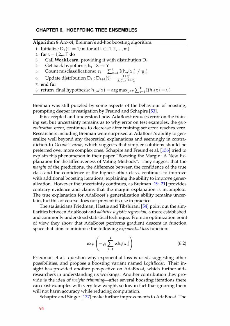
CHAPTER 6. HOEFFDING TREE ENSEMBLES
Algorithm 8 Arc-x4, Breiman’s ad-hoc boosting algorithm.1: Initialize D1(i) = 1/m for all i ∈ {1, 2, ...,m}
2: for t = 1,2,...T do3: Call WeakLearn, providing it with distribution Dt4: Get back hypothesis ht : X→ Y
5: Count misclassifications: ei =∑tn=1 I(hn(xi) 6= yi)
6: Update distribution Dt : Dt+1(i) =1+e4
i∑mn=1 1+e
4n
7: end for8: return final hypothesis: hfin(x) = arg maxy∈Y
∑Tt=1 I(ht(x) = y)
Breiman was still puzzled by some aspects of the behaviour of boosting,prompting deeper investigation by Freund and Schapire [53].
It is accepted and understood how AdaBoost reduces error on the train-ing set, but uncertainty remains as to why error on test examples, the gen-eralization error, continues to decrease after training set error reaches zero.Researchers including Breiman were surprised at AdaBoost’s ability to gen-eralize well beyond any theoretical explanations and seemingly in contra-diction to Occam’s razor, which suggests that simpler solutions should bepreferred over more complex ones. Schapire and Freund et al. [136] tried toexplain this phenomenon in their paper “Boosting the Margin: A New Ex-planation for the Effectiveness of Voting Methods”. They suggest that themargin of the predictions, the difference between the confidence of the trueclass and the confidence of the highest other class, continues to improvewith additional boosting iterations, explaining the ability to improve gener-alization. However the uncertainty continues, as Breiman [19, 21] providescontrary evidence and claims that the margin explanation is incomplete.The true explanation for AdaBoost’s generalization ability remains uncer-tain, but this of course does not prevent its use in practice.
The statisticians Friedman, Hastie and Tibshirani [54] point out the sim-ilarities between AdaBoost and additive logistic regression, a more establishedand commonly understood statistical technique. From an optimization pointof view they show that AdaBoost performs gradient descent in functionspace that aims to minimise the following exponential loss function:
exp
(−yi
T∑t=1
αht(xi)
)(6.2)
Friedman et al. question why exponential loss is used, suggesting otherpossibilities, and propose a boosting variant named LogitBoost. Their in-sight has provided another perspective on AdaBoost, which further aidsresearchers in understanding its workings. Another contribution they pro-vide is the idea of weight trimming—after several boosting iterations therecan exist examples with very low weight, so low in fact that ignoring themwill not harm accuracy while reducing computation.
Schapire and Singer [137] make further improvements to AdaBoost. The
94

6.1. BATCH SETTING
original formulation only used binary votes of ensemble members to reweightexamples. The improved formulation generalizes the algorithm to makeuse of confidences output by base members, potentially improving perfor-mance. They show how to handle multiple class labels and also study howto best devise algorithms to output confidences suiting the improved Ad-aBoost. Additionally, they propose an alternative gain criterion, so that forexample, decision trees can be induced that aim to directly improve boost-ing performance.
Early enthusiasm for AdaBoost sometimes overlooked its shortcomings.Observing its spectacular ability to generalize on many data sets it wassometimes suggested that AdaBoost is resistant to overfitting. Dietterich [36]addressed such claims by demonstrating that AdaBoost can suffer fromproblems with noise. In fact, his experiments show that with substantialclassification noise, bagging is much better than boosting. The explanationfor this behaviour is that AdaBoost will inevitably give higher weight tonoisy examples, because they will consistently be misclassified.
An interesting piece of follow-up work was conducted by Freund [50],who revisited his boost-by-majority algorithm to make it adaptive like Ad-aBoost. The result is the BrownBoost algorithm. BrownBoost considers thelimit in which each boosting iteration makes an infinitesimally small contri-bution to the whole process, which can be modelled with Brownian motion.As with the original boost-by-majority, the number of iterations, T , is fixedin advance. The algorithm is optimized to minimize the training error inthe pre-assigned number of iterations—as the final iteration draws near, thealgorithm gives up on examples that are consistently misclassified. Thisoffers hope of overcoming the problems with noise that are suffered by Ad-aBoost. In fact, Freund shows that AdaBoost is a special case of BrownBoost,where T → ∞. Despite the theoretical benefits of BrownBoost it has failedto draw much attention from the community, perhaps because it is muchmore complicated and less intuitive than AdaBoost. The study [116] foundthat BrownBoost is more robust than AdaBoost in class noise, but that Log-itBoost performs at a comparable level.
6.1.3 Option Trees
Standard decision trees have only a single path that each example can fol-low1, so any given example will apply to only one leaf in the tree. Op-tion trees, introduced by Buntine [25] and further explored by Kohavi andKunz [104], are more general, making it possible for an example to traveldown multiple paths and arrive at multiple leaves. This is achieved by in-troducing the possibility of option nodes to the tree, alongside the standarddecision nodes and leaf nodes. An option node splits the decision path sev-eral ways—when an option node is encountered several different subtreesare traversed, which could themselves contain more option nodes, thus the
1For simplicity, this statement ignores missing value approaches such as C4.5 that sendexamples down several paths when testing on unknown attribute values.
95

CHAPTER 6. HOEFFDING TREE ENSEMBLES
potential for reaching different leaves is multiplied by every option. Mak-ing a decision with an option tree involves combining the predictions of theapplicable leaves into a final result.
Option trees are a single general structure that can represent anythingfrom a single standard decision tree to an ensemble of standard decisiontrees to an even more general tree containing options within options. Anoption tree without any option nodes is clearly the same as a standard de-cision tree. An option tree with only a single option node at the root canrepresent an ensemble of standard trees. Option nodes below other optionnodes take this a step further and have the combinational power to repre-sent many possible decision trees in a single compact structure.
A potential benefit of option trees over a traditional ensemble is that themore flexible representation can save space—consider as an extreme exam-ple an ensemble of one hundred mostly identical large trees, where the onlydifference between each tree lies at a single leaf node, in the same positionin each tree. The standard ensemble representation would require one hun-dred whole copies of the tree where only the leaf would differ. Efficientlyrepresented as an option tree this would require almost a hundred times lessspace, where the varying leaf could be replaced by an option node splittingone hundred ways leading to the one hundred different leaf variants. Thedrive for diverse ensembles will of course make such a scenario unlikely,but the illustration serves the point that there are savings to be made bycombining different tree permutations into a single structure. Essentiallyevery path above an option node can be saved from repetition in memory,compared to explicitly storing every individual tree found in combination.
Another possible benefit offered by option trees is retention of inter-pretability. An accepted disadvantage of ensemble methods is that userswill lose the ability to understand the models produced. An option tree isa single structure, and in some situations this can aid in interpreting thedecision process, much more so than trying to determine the workings ofseveral completely separate models in combination. An option tree con-taining many options at many levels can be complex, but humans may notbe as confused by a limited number of option nodes in small and simpleoption trees. Arguments for the interpretability of option trees can be foundin [104, 51].
In terms of accuracy, an option tree is just as capable of increasing accu-racy as any ensemble technique. Depending on how it is induced, an optiontree could represent the result of bagging or boosting trees, or somethingelse entirely. An example application of boosting to option tree inductionis the alternating decision tree (ADTree) learning algorithm by Freund andMason [51].
The option tree induction approach by Kohavi and Kunz [104] seeks toexplore and average additional split possibilities that a tree could make.Their approach is closer to bagging than boosting, because bagging alsodraws out different possibilities from the trees, but operates in a randomand less direct fashion. It is less like boosting because it does not utilize clas-
96
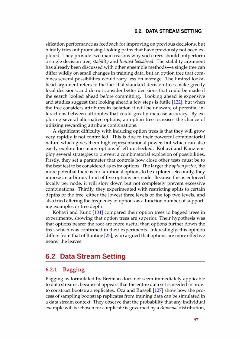
6.2. DATA STREAM SETTING
sification performance as feedback for improving on previous decisions, butblindly tries out promising-looking paths that have previously not been ex-plored. They provide two main reasons why such trees should outperforma single decision tree, stability and limited lookahead. The stability argumenthas already been discussed with other ensemble methods—a single tree candiffer wildly on small changes in training data, but an option tree that com-bines several possibilities would vary less on average. The limited looka-head argument refers to the fact that standard decision trees make greedylocal decisions, and do not consider better decisions that could be made ifthe search looked ahead before committing. Looking ahead is expensiveand studies suggest that looking ahead a few steps is futile [122], but whenthe tree considers attributes in isolation it will be unaware of potential in-teractions between attributes that could greatly increase accuracy. By ex-ploring several alternative options, an option tree increases the chance ofutilizing rewarding attribute combinations.
A significant difficulty with inducing option trees is that they will growvery rapidly if not controlled. This is due to their powerful combinatorialnature which gives them high representational power, but which can alsoeasily explore too many options if left unchecked. Kohavi and Kunz em-ploy several strategies to prevent a combinatorial explosion of possibilities.Firstly, they set a parameter that controls how close other tests must be tothe best test to be considered as extra options. The larger the option factor, themore potential there is for additional options to be explored. Secondly, theyimpose an arbitrary limit of five options per node. Because this is enforcedlocally per node, it will slow down but not completely prevent excessivecombinations. Thirdly, they experimented with restricting splits to certaindepths of the tree, either the lowest three levels or the top two levels, andalso tried altering the frequency of options as a function number of support-ing examples or tree depth.
Kohavi and Kunz [104] compared their option trees to bagged trees inexperiments, showing that option trees are superior. Their hypothesis wasthat options nearer the root are more useful than options further down thetree, which was confirmed in their experiments. Interestingly, this opiniondiffers from that of Buntine [25], who argued that options are more effectivenearer the leaves.
6.2 Data Stream Setting
6.2.1 Bagging
Bagging as formulated by Breiman does not seem immediately applicableto data streams, because it appears that the entire data set is needed in orderto construct bootstrap replicates. Oza and Russell [127] show how the pro-cess of sampling bootstrap replicates from training data can be simulated ina data stream context. They observe that the probability that any individualexample will be chosen for a replicate is governed by a Binomial distribution,
97

CHAPTER 6. HOEFFDING TREE ENSEMBLES
so the sampling process can be approximated by considering each exam-ple in turn and randomly deciding with a Binomial probability distributionhow many times to include the example in the formation of a replicate set.The difficulty with this solution is that the number of examples, N, needsto be known in advance. Oza and Russell get around this by consideringwhat happens when N → ∞, which is a reasonable assumption to makewith data streams of arbitrary length, and conclude that the Binomial distri-bution tends to a Poisson(1) distribution. Following these observations thealgorithm is straightforward to implement, listed in Algorithm 9. It requiresa base learner that is also capable of processing data streams.
Algorithm 9 Oza and Russell’s Online Bagging. M is the number of modelsin the ensemble and I(·) is the indicator function.
1: Initialize base models hm for allm ∈ {1, 2, ...,M}
2: for all training examples do3: form = 1, 2, ...,M do4: Set k = Poisson(1)5: for n = 1, 2, ..., k do6: Update hm with the current example7: end for8: end for9: end for
10: anytime output:11: return hypothesis: hfin(x) = arg maxy∈Y
∑Tt=1 I(ht(x) = y)
Oza and Russell construct proofs to demonstrate that their “online” bag-ging algorithm converges towards the original batch algorithm [127], andhave collected experimental evidence to show this [126]. One issue theyhave not addressed is memory management, a consideration that is paramountin this text. Assuming that a memory-limited base algorithm is available,such as the Hoeffding tree algorithm studied in Chapter 3, then the memoryrequirements of an ensemble of trees can be controlled by limits on individ-ual members. The experimental implementation of bagged Hoeffding treestakes a simple approach to controlling total memory usage—with an overallmemory limit of m and a total of n trees, each tree is limited to a maximumsize ofm/n.
6.2.2 Boosting
Existing literature for the problem of applying boosting to data stream clas-sification has mainly focussed on modifying AdaBoost, and often under theguise of online learning [127, 44]. The term “online” is slightly ambiguous, asresearchers have used it in the past to refer to varying goals. Typically thefocus is on processing a single example at a time, but sometimes withoutemphasis on other factors believed important in this text such as memory
98
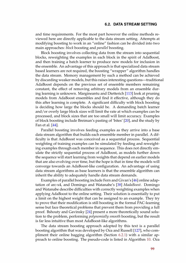
6.2. DATA STREAM SETTING
and time requirements. For the most part however the online methods re-viewed here are directly applicable to the data stream setting. Attempts atmodifying boosting to work in an “online” fashion can be divided into twomain approaches: block boosting and parallel boosting.
Block boosting involves collecting data from the stream into sequentialblocks, reweighting the examples in each block in the spirit of AdaBoost,and then training a batch learner to produce new models for inclusion inthe ensemble. An advantage of this approach is that specialized data streambased learners are not required, the boosting “wrapper” algorithm handlesthe data stream. Memory management by such a method can be achievedby discarding weaker models, but this raises interesting questions—traditionalAdaBoost depends on the previous set of ensemble members remainingconstant, the effect of removing arbitrary models from an ensemble dur-ing learning is unknown. Margineantu and Dietterich [113] look at pruningmodels from AdaBoost ensembles and find it effective, although they dothis after learning is complete. A significant difficulty with block boostingis deciding how large the blocks should be. A demanding batch learnerand/or overly large block sizes will limit the rate at which examples can beprocessed, and block sizes that are too small will limit accuracy. Examplesof block boosting include Breiman’s pasting of ‘bites’ [20], and the study byFan et al. [44].
Parallel boosting involves feeding examples as they arrive into a basedata stream algorithm that builds each ensemble member in parallel. A dif-ficulty is that AdaBoost was conceived as a sequential process. Sequentialweighting of training examples can be simulated by feeding and reweight-ing examples through each member in sequence. This does not directly em-ulate the strictly sequential process of AdaBoost, as models further downthe sequence will start learning from weights that depend on earlier modelsthat are also evolving over time, but the hope is that in time the models willconverge towards an AdaBoost-like configuration. An advantage of usingdata stream algorithms as base learners is that the ensemble algorithm caninherit the ability to adequately handle data stream demands.
Examples of parallel boosting include Fern and Givan’s [46] online adap-tation of arc-x4, and Domingo and Watanabe’s [38] MadaBoost. Domingoand Watanabe describe difficulties with correctly weighting examples whenapplying AdaBoost to the online setting. Their solution is essentially to puta limit on the highest weight that can be assigned to an example. They tryto prove that their modification is still boosting in the formal PAC-learningsense but face theoretical problems that prevent them from providing a fullproof. Bshouty and Gavinsky [24] present a more theoretically sound solu-tion to the problem, performing polynomially smooth boosting, but the resultis far less intuitive than most AdaBoost-like algorithms.
The data stream boosting approach adopted by this text is a parallelboosting algorithm that was developed by Oza and Russell [127], who com-pliment their online bagging algorithm (Section 6.2.1) with a similar ap-proach to online boosting. The pseudo-code is listed in Algorithm 10. Oza
99

CHAPTER 6. HOEFFDING TREE ENSEMBLES
Algorithm 10 Oza and Russell’s Online Boosting. N is the number of exam-ples seen.
1: Initialize base models hm for allm ∈ {1, 2, ...,M}, λscm = 0, λswm = 0
2: for all training examples do3: Set “weight” of example λd = 1
4: form = 1, 2, ...,M do5: Set k = Poisson(λd)6: for n = 1, 2, ..., k do7: Update hm with the current example8: end for9: if hm correctly classifies the example then
10: λscm ← λscm + λd
11: λd ← λd
(N2λsc
m
)12: else13: λswm ← λswm + λd
14: λd ← λd
(N2λsw
m
)15: end if16: end for17: end for18: anytime output:19: Calculate εm = λsw
m
λscm +λsw
mand βm = εm/(1− εm) for allm ∈ {1, 2, ...,M}
20: return hypothesis: hfin(x) = arg maxy∈Y∑m:hm(x)=y log 1/βm
100

6.2. DATA STREAM SETTING
and Russell note that the weighting procedure of AdaBoost actually dividesthe total example weight into two halves—half of the weight is assignedto the correctly classified examples, and the other half goes to the misclas-sified examples. As the ensemble gets more accurate the number of mis-classified examples should progressively get less and less relative to thenumber of correct classifications. In turn, the misclassified set gets moreweight per example than the correctly classified set. This motivates theweight update procedure in lines 9-15, which is intended to simulate thebatch weight behaviour in a streaming environment, much like the onlinebagging algorithm is designed to simulate the creation of bootstrap repli-cates. Once again they utilize the Poisson distribution for deciding the ran-dom probability that an example is used for training, only this time the pa-rameter (λd) changes according to the boosting weight of the example as it ispassed through each model in sequence. The use of random Poisson is wellfounded for bagging, but motivation for it in the boosting situation is lessclear. Preliminary experimental work for this text involved testing severalboosting algorithms, including a modification of Oza and Russell’s boostingalgorithm that applied example weights directly instead of relying on ran-dom drawings from Poisson. Overall the algorithm performed better withthe random Poisson element than without it, so it seems to be a worthwhileapproach even if the theoretical underpinning is weak.
6.2.3 Option Trees
A new algorithm for inducing option trees from data streams was devisedfor this text. It is based on the Hoeffding tree induction algorithm, but gen-eralized to explore additional options in a manner similar to the option treesof Kohavi and Kunz [104]. The pseudo-code is listed in Algorithm 11. Thealgorithm is an extension of the basic decision tree inducer listed in Algo-rithm 2 on page 50. The differences are, firstly, that each training examplecan update a set of option nodes rather than just a single leaf, and secondly,lines 20-32 constitute new logic that applies when a split has already beenchosen but extra options are still being considered.
A minor point of difference between Kohavi and Kunz’s option tree andthe Hoeffding option trees implemented for this study is that the Hoeffdingoption tree uses the class confidences in each leaf to help form the majoritydecision. The observed probabilities of each class are added together, ratherthan the binary voting process used by Kohavi and Kunz where each leafvotes completely towards the local majority in determining the overall ma-jority label. Preliminary experiments suggested that using confidences invoting can slightly improve accuracy.
Just as Kohavi and Kunz needed to restrict the growth of their optiontrees in the batch setting, strategies are required to control the growth ofHoeffding option trees. Without any restrictions the tree will try to exploreall possible tree configurations simultaneously which is clearly not feasible.
The first main approach to controlling growth involves the initial deci-
101

CHAPTER 6. HOEFFDING TREE ENSEMBLES
Algorithm 11 Hoeffding option tree induction algorithm. δ ′ is the confi-dence for additional splits and maxOptions is the maximum number ofoptions that should be reachable by any single example.
1: Let HOT be an option tree with a single leaf (the root)2: for all training examples do3: Sort example into leaves/option nodes L using HOT4: for all option nodes l of the set L do5: Update sufficient statistics in l6: Increment nl, the number of examples seen at l7: if nl mod nmin = 0 and examples seen at l not all of same class
then8: if l has no children then9: Compute Gl(Xi) for each attribute
10: Let Xa be attribute with highest Gl11: Let Xb be attribute with second-highest Gl12: Compute Hoeffding bound ε =
√R2ln(1/δ)2nl
13: if Xa 6= X∅ and (Gl(Xa) −Gl(Xb) > ε or ε < τ) then14: Add a node below l that splits on Xa15: for all branches of the split do16: Add a new option leaf with initialized sufficient statistics17: end for18: end if19: else20: if optionCountl < maxOptions then21: Compute Gl(Xi) for existing splits and (non-used) attributes
22: Let S be existing child split with highest Gl23: Let X be (non-used) attribute with highest Gl24: Compute Hoeffding bound ε =
√R2ln(1/δ ′)
2nl
25: if Gl(X) −Gl(S) > ε then26: Add an additional child option to l that splits on X27: for all branches of the split do28: Add a new option leaf with initialized sufficient statis-
tics29: end for30: end if31: else32: Remove attribute statistics stored at l33: end if34: end if35: end if36: end for37: end for
102

6.2. DATA STREAM SETTING
sion of when to introduce new options to the tree. Kohavi and Kunz havean option factor parameter that controls the inducer’s eagerness to add newoptions. The Hoeffding option tree algorithm has a similar parameter, δ ′,which can be thought of as a secondary Hoeffding bound confidence. Theδ ′ parameter controls the confidence of secondary split decisions much likeδ influences the initial split decision, only for additional splits the test iswhether the information gain of the best candidate exceeds the informationgain of the best split already present in the tree. For the initial split, thedecision process searches for the best attribute overall, but for subsequentsplits, the search is for attributes that are superior to existing splits. It isvery unlikely that any other attribute could compete so well with the bestattribute already chosen that it could beat it by the same initial margin. Re-call, the original Hoeffding bound decision is designed to guarantee thatthe other attributes should not be any better. For this reason, the secondarybound δ ′ needs to be much looser than the initial bound δ for there to beany chance of additional attribute choices. It seems a contradiction to re-quire other attributes to be better when the Hoeffding bound has alreadyguaranteed with high confidence that they are not as good, but the guaran-tees are much weaker when tie breaking has been employed, and setting asufficiently loose secondary bound does indeed create further split options.δ ′ can be expressed in terms of a multiplication factor α, specifying a frac-tion of the original Hoeffding bound:
δ ′ = eα2 ln(δ) (6.3)
Or equivalently:
α =
√ln(δ ′)
ln(δ)(6.4)
For example, with the default parameter settings of δ = 10−7 and δ ′ = 0.999
then from Equation 6.4, α ≈ 0.0079, that is, decisions to explore additionalattributes are approximately 126 times more eager than the initial choice ofattribute. Preliminary experiments found that a setting of δ ′ = 0.999 workswell in combination with the second overriding growth strategy discussednext.
The second main approach to controlling tree growth involves directlylimiting the number of options that the tree will explore. Kohavi and Kunztried a local limit, where they would not allow an option node to split morethan five different ways. This text introduces a global limiting strategy thatinstead of limiting options per node it limits options per example. A combina-torial explosion is still possible with a locally applied limit, whereas a globallimit prevents it altogether. Doing so requires more work to compute howmany leaves are reachable at a particular point in the tree, and only allowingmore options if it does not exceed the maximum allowed. Line 20 of Algo-rithm 11 performs the test that determines whether more options are possi-ble, and assumes that the maximum reachability count (optionCountl) of
103

CHAPTER 6. HOEFFDING TREE ENSEMBLES
86.4
86.6
86.8
87
87.2
87.4
87.6
87.8
88
1 2 3 4 5 6 7 8 9 10 11 12 13 14 15
aver
age
accu
racy
(%
cor
rect
)
maximum options per example
Figure 6.3: Average accuracy of Hoeffding option tree over many data setsversus the maximum number of options per example. Accuracies were es-timated in unbounded memory.
the node is available. Computing maximum reachability counts in an op-tion tree is complicated—it not only depends on the descendants of a nodebut also on its ancestors, and their descendants too. To solve this probleman incremental algorithm was devised to keep track of maximum counts ineach option node in the tree, listed in Algorithm 12. The worst-case com-plexity of this algorithm is linear in the number of nodes in the tree, as itcould potentially visit every node once. All nodes start with an optionCountof 1. The operation for updating counts is employed every time the treegrows. Nodes are not removed from the tree, as pruning is not consideredin this text. However, an operation for removing option nodes, that wouldbe needed if the option trees were pruned, is included for completeness.
Interestingly, the arbitrary local limit of five options employed by Kohaviand Kunz also seems to be a good choice for the global limit suggested here,at least when memory restrictions are not considered. Early experimentslooked at the effect of the maxOptions parameter on smaller scale runs inunbounded memory. The average accuracy across many data sets is plottedin Figure 6.3, showing that prior to a maximum of five options there aresignificant accuracy gains, but after that point the accuracy gains diminish.The computational demands continue to rise with each additional option.
Other design decisions also help to limit tree growth. When searchingfor additional options, ties are not broken in the same manner as during theinitial decision. Doing so would inevitably force options to be introducedwhen the bound is sufficiently small. Instead, this cuts down excessive op-
104

6.2. DATA STREAM SETTING
Algorithm 12 Option counter update, for adding and removing options.ProcedureAddOption(node, newOption):max← node.optionCount
if node has children thenmax← max+ 1
end iffor all children of newOption dochild.optionCount← max
end foradd newOption as child of nodecall UpdateOptionCount(node,newOption)
ProcedureRemoveOption(node, index):while there are options below node do
remove deepest optionend whileremove child at index from nodecall UpdateOptionCountBelow(node,-1)if node has parent then
call UpdateOptionCount(parent,node)end if
ProcedureUpdateOptionCount(node, source):max←maximum optionCount of node childrenδ← max− node.optionCount
if δ 6= 0 thennode.optionCount← node.optionCount+ δ
for all children of node such that child 6= source docall UpdateOptionCountBelow(child,δ)
end forif node has parent then
call UpdateOptionCount(parent,node)end if
end if
ProcedureUpdateOptionCountBelow(node, δ):node.optionCount← node.optionCount+ δ
for all children of node docall UpdateOptionCountBelow(child, δ)
end for
105

CHAPTER 6. HOEFFDING TREE ENSEMBLES
tions by only considering genuine contenders that emerge, those with pos-itive gains. Another restriction is that an attribute will only be used onceper option node, which reduces the possibility of multiple redundant splits,especially where numeric attributes are concerned.
Having internal nodes that also act like active leaves because they recordsufficient statistics has serious implications for memory management. Toreduce the memory requirements of internal nodes, they are deactivated assoon as further options are prohibited (line 32 of Algorithm 11). The mem-ory management strategy needs to be adapted to cope with these costlynodes when memory is exhausted. Recall from Section 3.3 that each leafhas a measure of ‘promise’. The least promising nodes are deactivated first,while the most promising are retained in memory the longest. The ‘promise’is measured by the numbers of examples seen by the node since creation thatare not correctly classified by the majority observed class. Three straightfor-ward approaches were compared to decide the final method for experimen-tal comparison:
1. Each active node is treated equally, regardless of whether it is internalor a leaf. This has the most potential to stall growth because too manyinternal leaves that are highly promising will prevent the tree fromgrowing at the leaves. Also, nodes near the top of the tree such as theroot node are likely to always look promising due to high numbers ofmisclassified examples at that point.
2. Internal nodes are penalized by dividing their promise by the num-ber of local options. This reduces focus on areas that have alreadyexplored several options.
3. Leaf nodes are always more promising than internal nodes. This meansthat when reclaiming memory the internal nodes are always the first tobe removed, in order of promise. Once all internal nodes are removed,the leaf nodes will start being deactivated, in the same manner as stan-dard Hoeffding trees.
The third option fared the best, and is the strategy used in experiments. Itappears that seeking more options at the expense of pursuing the existingones is harmful overall to tree accuracy.
The maxOptions parameter plays a significant role overall when memoryis limited, because it adjusts the tradeoff between the numbers of optionsthat are explored and the depth at which they can be explored.
6.3 Realistic Ensemble Sizes
In the batch setting, a typical ensemble may consist of one hundred or morebase models. This is because the primary goal is increasing accuracy, andthe more models combined the greater the potential for this to occur. Thememory and computational implications of combining this many models
106

6.3. REALISTIC ENSEMBLE SIZES
in the batch setting are not a major concern, as typically training sizes aresmall, and prolonged training and testing times are acceptable. If it weretoo demanding, there is always the option to use a simpler base algorithmor reduce the ensemble size.
In the data stream setting the extra demands of combining models mustbe carefully considered. If a particular algorithm is barely able to cope witha high-speed stream, then even adding a second model in parallel will not befeasible. For every additional model included, the gains must be weighedagainst the cost of supporting them. An ensemble of one hundred mod-els would process examples approximately one hundred times slower, andmemory restrictions would require each model to be one hundred times assmall. In 100KB of memory this would rely heavily on memory manage-ment, which would endeavour to keep each model under 1KB in size. Ifsensible models can be induced in such conditions, the simplistic modelsmay not work as effectively in combination than more sophisticated ones.For these reasons, the ensemble sizes experimented with in the next chapterare restricted to smaller values of ten, five or three models.
Such small ensemble sizes are not necessarily a hindrance to ensembleperformance. The preliminary investigation into restricting the effectivenumber of models in option trees, Figure 6.3, suggested that anything on theorder of five models is close to optimal, and that higher numbers of modelsshow limited improvement. This was without considering the added pres-sure of memory limits, which in some conditions may favour even smallercombinations. The ensemble size of three especially will be an interestingstudy of whether small combinations can show a useful effect.
107


Part III
Evolving Data Stream Learning
109

7Evolving data streams
Data mining has traditionally been performed over static datasets, wheredata mining algorithms can afford to read the input data several times.When the source of data items is an open-ended data stream, not all datacan be loaded into the memory and off-line mining with a fixed size datasetis no longer technically feasible due to the unique features of streaming data.
The following constraints apply in the Data Stream model:
1. The amount of data that has arrived and will arrive in the future isextremely large; in fact, the sequence is potentially infinite. Thus, itis impossible to store it all. Only a small summary can be computedand stored, and the rest of the information is thrown away. Even if theinformation could be all stored, it would be unfeasible to go over it forfurther processing.
2. The speed of arrival is large, so that each particular element has to beprocessed essentially in real time, and then discarded.
3. The distribution generating the items can change over time. Thus,data from the past may become irrelevant (or even harmful) for thecurrent summary.
Constraints 1 and 2 limit the amount of memory and time-per-item thatthe streaming algorithm can use. Intense research on the algorithmics ofData Streams has produced a large body of techniques for computing fun-damental functions with low memory and time-per-item, usually in combi-nation with the sliding-window technique discussed next.
Constraint 3, the need to adapt to time changes, has been also intenselystudied. A typical approach for dealing is based on the use of so-calledsliding windows: The algorithm keeps a window of size W containing thelast W data items that have arrived (say, in the last W time steps). Whena new item arrives, the oldest element in the window is deleted to makeplace for it. The summary of the Data Stream is at every moment computedor rebuilt from the data in the window only. If W is of moderate size, thisessentially takes care of the requirement to use low memory.
In most cases, the quantity W is assumed to be externally defined, andfixed through the execution of the algorithm. The underlying hypothesis isthat the user can guessW so that the distribution of the data can be thought
111

CHAPTER 7. EVOLVING DATA STREAMS
to be essentially constant in most intervals of sizeW; that is, the distributionchanges smoothly at a rate that is small w.r.t. W, or it can change drasticallyfrom time to time, but the time between two drastic changes is often muchgreater thanW.
Unfortunately, in most of the cases the user does not know in advancewhat the rate of change is going to be, so its choice of W is unlikely to beoptimal. Not only that, the rate of change can itself vary over time, so theoptimalW may itself vary over time.
7.1 Algorithms for mining with change
In this section we review some of the data mining methods that deal withdata streams and concept drift. There are many algorithms in the literaturethat address this problem. We focus on the ones that they are more referredto in other works.
7.1.1 OLIN: Last
Last in [108] describes an online classification system that uses the info-fuzzy network (IFN). The system called OLIN (On Line Information Net-work) gets a continuous stream of non-stationary data and builds a networkbased on a sliding window of the latest examples. The system dynami-cally adapts the size of the training window and the frequency of modelre-construction to the current rate of concept drift
OLIN uses the statistical significance of the difference between the train-ing and the validation accuracy of the current model as an indicator of con-cept stability.
OLIN adjusts dynamically the number of examples between model re-constructions by using the following heuristic: keep the current model formore examples if the concept appears to be stable and reduce drastically thesize of the validation window, if a concept drift is detected.
OLIN generates a new model for every new sliding window. This ap-proach ensures accurate and relevant models over time and therefore anincrease in the classification accuracy. However, the OLIN algorithm hasa major drawback, which is the high cost of generating new models. OLINdoes not take into account the costs involved in replacing the existing modelwith a new one.
7.1.2 CVFDT: Domingos
Hulten, Spencer and Domingos presented Concept-adapting Very Fast De-cision Trees CVFDT [86] algorithm as an extension of VFDT to deal withconcept change.
Figure 7.1 shows CVFDT algorithm. CVFDT keeps the model it is learn-ing in sync with such changing concepts by continuously monitoring the
112

7.1. ALGORITHMS FOR MINING WITH CHANGE
quality of old search decisions with respect to a sliding window of data fromthe data stream, and updating them in a fine-grained way when it detectsthat the distribution of data is changing. In particular, it maintains sufficientstatistics throughout time for every candidateM considered at every searchstep. After the first w examples, where w is the window width, it subtractsthe oldest example from these statistics whenever a new one is added. Af-ter every ∆n new examples, it determines again the best candidates at everyprevious search decision point. If one of them is better than an old winnerby δ∗ then one of two things has happened. Either the original decision wasincorrect (which will happen a fraction δ of the time) or concept drift hasoccurred. In either case,it begins an alternate search starting from the newwinners, while continuing to pursue the original search. Periodically it usesa number of new examples as a validation set to compare the performanceof the models produced by the new and old searches. It prunes an old search(and replace it with the new one) when the new model is on average betterthan the old one, and it prunes the new search if after a maximum numberof validations its models have failed to become more accurate on averagethan the old ones. If more than a maximum number of new searches is inprogress, it prunes the lowest-performing ones.
7.1.3 UFFT: Gama
Gama, Medas and Rocha [58] presented the Ultra Fast Forest of Trees (UFFT)algorithm.
UFFT is an algorithm for supervised classification learning, that gener-ates a forest of binary trees. The algorithm is incremental, processing eachexample in constant time, works on-line, UFFT is designed for continuousdata. It uses analytical techniques to choose the splitting criteria, and theinformation gain to estimate the merit of each possible splitting-test. Formulti-class problems, the algorithm builds a binary tree for each possiblepair of classes leading to a forest-of-trees. During the training phase thealgorithm maintains a short term memory. Given a data stream, a limitednumber of the most recent examples are maintained in a data structure thatsupports constant time insertion and deletion. When a test is installed, aleaf is transformed into a decision node with two descendant leaves. Thesufficient statistics of the leaf are initialized with the examples in the shortterm memory that will fall at that leaf.
The UFFT algorithm maintains, at each node of all decision trees, a NaıveBayes classifier. Those classifiers were constructed using the sufficient statis-tics needed to evaluate the splitting criteria when that node was a leaf. Afterthe leaf becomes a node, all examples that traverse the node will be classi-fied by the Naıve Bayes. The basic idea of the drift detection method isto control this error-rate. If the distribution of the examples is stationary,the error rate of Naıve-Bayes decreases. If there is a change on the distri-bution of the examples the Naıve Bayes error increases. The system usesDDM, the drift detection method explained in Section 1.5. When it detects
113

CHAPTER 7. EVOLVING DATA STREAMS
CVFDT(Stream, δ)
1 Let HT be a tree with a single leaf(root)2 Init counts nijk at root3 for each example (x, y) in Stream4 do Add, Remove and Forget Examples5 CVFDTGROW((x, y), HT, δ)
6 CHECKSPLITVALIDITY(HT,n, δ)
CVFDTGROW((x, y), HT, δ)
1 Sort (x, y) to leaf l using HT2 Update counts nijk at leaf l and nodes traversed in the sort3 if examples seen so far at l are not all of the same class4 then Compute G for each attribute
5 if G(Best Attr.)−G(2nd best) >√
R2 ln 1/δ2n
6 then Split leaf on best attribute7 for each branch8 do Start new leaf and initialize counts9 Create alternate subtree
CHECKSPLITVALIDITY(HT,n, δ)
1 for each node l in HT that it is not a leaf2 do for each tree Talt in ALT(l)3 do CHECKSPLITVALIDITY(Talt, n, δ)
4 if exists a new promising attributes at node l5 do Start an alternate subtree
Figure 7.1: The CVFDT algorithm
114

7.2. A METHODOLOGY FOR ADAPTIVE STREAM MINING
an statistically significant increase of the Naıve-Bayes error in a given node,an indication of a change in the distribution of the examples, this suggestthat the splitting-test that has been installed at this node is no longer appro-priate. The subtree rooted at that node is pruned, and the node becomesa leaf. All the sufficient statistics of the leaf are initialized. When a newtraining example becomes available, it will cross the corresponding binarydecision trees from the root node till a leaf. At each node, the Naıve Bayesinstalled at that node classifies the example. The example will be correctlyor incorrectly classified. For a set of examples the error is a random variablefrom Bernoulli trials. The Binomial distribution gives the general form ofthe probability for the random variable that represents the number of errorsin a sample of n examples.
The sufficient statistics of the leaf are initialized with the examples inthe short term memory that maintains a limited number of the most re-cent examples. It is possible to observe an increase of the error reachingthe warning level, followed by a decrease. This method uses the informa-tion already available to the learning algorithm and does not require addi-tional computational resources. An advantage of this method is it contin-uously monitors the online error of Naıve Bayes. It can detect changes inthe class-distribution of the examples at any time. All decision nodes con-tain Naıve Bayes to detect changes in the class distribution of the examplesthat traverse the node, that correspond to detect shifts in different regionsof the instance space. Nodes near the root should be able to detect abruptchanges in the distribution of the examples, while deeper nodes should de-tect smoothed changes.
7.2 A Methodology for Adaptive Stream Mining
In the data stream mining literature, most algorithms incorporate one ormore of the following ingredients: windows to remember recent examples;methods for detecting distribution change in the input; and methods forkeeping updated estimations for some statistics of the input. We see themas the basis for solving the three central problems of
• what to remember or forget,
• when to do the model upgrade, and
• how to do the model upgrade.
Our claim is that by basing mining algorithms on well-designed, well-encapsulated modules for these tasks, one can often get more generic andmore efficient solutions than by using ad-hoc techniques as required.
115

CHAPTER 7. EVOLVING DATA STREAMS
-xt
Estimator- -
AlarmChange Detector
-Estimation
Memory-
6
6?
Figure 7.2: General Framework
7.2.1 Time Change Detectors and Predictors: A General Frame-work
Most approaches for predicting and detecting change in streams of data canbe discussed in the general framework: The system consists of three mod-ules: a Memory module, an Estimator Module, and a Change Detector orAlarm Generator module. These three modules interact as shown in Fig-ure 7.2, which is analogous to Figure 8 in [139].In general, the input to this algorithm is a sequence x1, x2, . . . , xt, . . . of dataitems whose distribution varies over time in an unknown way. The outputsof the algorithm are, at each time step
• an estimation of some important parameters of the input distribution,and
• a signal alarm indicating that distribution change has recently occurred.
We consider a specific, but very frequent case, of this setting: that inwhich all the xt are real values. The desired estimation is usually the ex-pected value of the current xt, and less often another distribution statisticssuch as the variance. The only assumption on the distribution is that eachxt is drawn independently from each other.
Memory is the component where the algorithm stores all the sample dataor summary that considers relevant at current time, that is, that presumablyshows the current data distribution.
The Estimator component is an algorithm that estimates the desired statis-tics on the input data, which may change over time. The algorithm mayor may not use the data contained in the Memory. The simplest Estima-tor algorithm for the expected is the linear estimator, which simply returnsthe average of the data items contained in the Memory. Other examples ofrun-time efficient estimators are Auto-Regressive, Auto Regressive MovingAverage, and Kalman filters.
The change detector component outputs an alarm signal when it detectschange in the input data distribution. It uses the output of the Estimator,and may or may not in addition use the contents of Memory.
116

7.2. A METHODOLOGY FOR ADAPTIVE STREAM MINING
In Table 7.1 we classify these predictors in four classes, depending onwhether Change Detector and Memory modules exist:
No memory Memory
Type I Type IIINo Change Detector Kalman Filter Adaptive Kalman Filter
Type II Type IVChange Detector Kalman Filter + CUSUM ADWIN
Kalman Filter + ADWIN
Table 7.1: Types of Time Change Predictor and some examples
• Type I: Estimator only. The simplest one is modelled by
xk = (1− α)xk−1 + α · xk.
The linear estimator corresponds to using α = 1/N where N is thewidth of a virtual window containing the last N elements we wantto consider. Otherwise, we can give more weight to the last elementswith an appropriate constant value of α. The Kalman filter tries tooptimize the estimation using a non-constant α (the K value) whichvaries at each discrete time interval.
• Type II: Estimator with Change Detector. An example is the Kalman Filtertogether with a CUSUM test change detector algorithm, see for exam-ple [91].
• Type III: Estimator with Memory. We add Memory to improve the resultsof the Estimator. For example, one can build an Adaptive KalmanFilter that uses the data in Memory to compute adequate values forthe process variance Q and the measure variance R. In particular, onecan use the sum of the last elements stored into a memory window tomodel the Q parameter and the difference of the last two elements toestimate parameter R.
• Type IV: Estimator with Memory and Change Detector. This is the mostcomplete type. Two examples of this type, from the literature, are:
– A Kalman filter with a CUSUM test and fixed-length windowmemory, as proposed in [139]. Only the Kalman filter has accessto the memory.
117

CHAPTER 7. EVOLVING DATA STREAMS
– A linear Estimator over fixed-length windows that flushes whenchange is detected [99], and a change detector that compares therunning windows with a reference window.
In Chapter 8, we will present ADWIN, an adaptive sliding windowmethod that works as a type IV change detector and predictor.
7.2.2 Window Management Models
Window strategies have been used in conjunction with mining algorithmsin two ways: one, externally to the learning algorithm; the window systemis used to monitor the error rate of the current model, which under stabledistributions should keep decreasing or at most stabilize; when instead thisrate grows significantly, change is declared and the base learning algorithmis invoked to revise or rebuild the model with fresh data. Note that in thiscase the window memory contains bits or real numbers (not full examples).Figure 7.3 shows this model.
The other way is to embed the window system inside the learning algo-rithm, to maintain the statistics required by the learning algorithm continu-ously updated; it is then the algorithm’s responsibility to keep the model insynchrony with these statistics, as shown in Figure 7.4.
-input output
DM Algorithm
Static Model
-
Change Detect.-
6
�
Figure 7.3: Data mining algorithm framework with concept drift.
Learning algorithms that detect change, usually compare statistics oftwo windows. Note that the methods may be memoryless: they may keepwindow statistics without storing all their elements. There have been in theliterature, some different window management strategies:
• Equal & fixed size subwindows: Kifer et al. [99] compares one refer-ence, non-sliding, window of older data with a sliding window of thesame size keeping the most recent data.
• Equal size adjacent subwindows: Dasu et al. [31] compares two adja-cent sliding windows of the same size of recent data.
118

7.2. A METHODOLOGY FOR ADAPTIVE STREAM MINING
-input output
DM Algorithm
-
Estimator1
Estimator2
Estimator3
Estimator4
Estimator5
Figure 7.4: Data mining algorithm framework with concept drift using esti-mators replacing counters.
• Total window against subwindow: Gama et al. [57] compares the win-dow that contains all the data with a subwindow of data from thebeginning until it detects that the accuracy of the algorithm decreases.
The strategy of ADWIN, the method presented in next chapter, will be tocompare all the adjacent subwindows in which is possible to partition thewindow containing all the data. Figure 7.5 shows these window manage-ment strategies.
LetW = 101010110111111
• Equal & fixed size subwindows: 1010 1011011 1111
• Equal size adjacent subwindows: 1010101 1011 1111
• Total window against subwindow: 10101011011 1111
• ADWIN: All adjacent subwindows:
1 01010110111111
1010 10110111111
1010101 10111111
1010101101 11111
10101011011111 1
Figure 7.5: Different window management strategies
119

CHAPTER 7. EVOLVING DATA STREAMS
7.3 Optimal Change Detector and Predictor
We have presented in section 7.2 a general framework for time change de-tectors and predictors. Using this framework we can establish the mainproperties of an optimal change detector and predictor system as the fol-lowing:
• High accuracy
• Fast detection of change
• Low false positives and negatives ratios
• Low computational cost: minimum space and time needed
• Theoretical guarantees
• No parameters needed
• Detector of type IV: Estimator with Memory and Change Detector
In the next chapter we will present ADWIN, a change detector and pre-dictor with these characteristics, using an adaptive sliding window model.ADWIN’s window management strategy will be to compare all the adjacentsubwindows in which is possible to partition the window containing all thedata. It seems that this procedure may be the most accurate, since it looksat all possible subwindows partitions. On the other hand, time cost is themain disadvantage of this method. Considering this, we will provide an-other version working in the strict conditions of the Data Stream model,namely low memory and low processing per item.
120

8Adaptive Sliding Windows
Dealing with data whose nature changes over time is one of the core prob-lems in data mining and machine learning. In this chapter we present ADWIN,an adaptive sliding window algorithm, as an estimator with memory andchange detector with the main properties of optimality explained in sec-tion 7.3. We study and develop also the combination of ADWIN with Kalmanfilters.
8.1 Introduction
Most strategies in the literature use variations of the sliding window idea:a window is maintained that keeps the most recently read examples, andfrom which older examples are dropped according to some set of rules. Thecontents of the window can be used for the three tasks: 1) to detect change(e.g., by using some statistical test on different subwindows), 2) obviously,to obtain updated statistics from the recent examples, and 3) to have data torebuild or revise the model(s) after data has changed.
The simplest rule is to keep a window of some fixed size, usually deter-mined a priori by the user. This can work well if information on the time-scale of change is available, but this is rarely the case. Normally, the useris caught in a tradeoff without solution: choosing a small size (so that thewindow reflects accurately the current distribution) and choosing a largesize (so that many examples are available to work on, increasing accuracyin periods of stability). A different strategy uses a decay function to weightthe importance of examples according to their age (see e.g. [30]): the relativecontribution of each data item is scaled down by a factor that depends onelapsed time. In this case, the tradeoff shows up in the choice of a decayconstant that should match the unknown rate of change.
Less often, it has been proposed to use windows of variable size. In gen-eral, one tries to keep examples as long as possible, i.e., while not provenstale. This delivers the users from having to guess a priori an unknownparameter such as the time scale of change. However, most works alongthese lines that we know of (e.g., [57, 101, 108, 157]) are heuristics andhave no rigorous guarantees of performance. Some works in computationallearning theory (e.g. [11, 78, 79]) describe strategies with rigorous perfor-mance bounds, but to our knowledge they have never been tried in real
121

CHAPTER 8. ADAPTIVE SLIDING WINDOWS
learning/mining contexts and often assume a known bound on the rate ofchange.
We will present ADWIN, a parameter-free adaptive size sliding window,with theoretical garantees. We will use Kalman filters at the last part of thisChapter, in order to provide an adaptive weight for each item.
8.2 Maintaining Updated Windows of Varying Length
In this section we describe algorithms for dynamically adjusting the lengthof a data window, make a formal claim about its performance, and derivean efficient variation.
We will use Hoeffding’s bound in order to obtain formal guarantees, anda streaming algorithm. However, other tests computing differences betweenwindow distributions may be used.
8.2.1 Setting
The inputs to the algorithms are a confidence value δ ∈ (0, 1) and a (pos-sibly infinite) sequence of real values x1, x2, x3, . . . , xt, . . . The value of xtis available only at time t. Each xt is generated according to some distribu-tion Dt, independently for every t. We denote with µt and σ2t the expectedvalue and the variance of xt when it is drawn according to Dt. We assumethat xt is always in [0, 1]; by an easy rescaling, we can handle any case inwhich we know an interval [a, b] such that a ≤ xt ≤ b with probability 1.Nothing else is known about the sequence of distributionsDt; in particular,µt and σ2t are unknown for all t.
8.2.2 First algorithm: ADWIN0
The first algorithm keeps a sliding window W with the most recently readxi. Let n denote the length ofW, µW the (observed) average of the elementsin W, and µW the (unknown) average of µt for t ∈ W. Strictly speaking,these quantities should be indexed by t, but in general t will be clear fromthe context.
Since the values of µt can oscillate wildly, there is no guarantee that µWor µW will be anywhere close to the instantaneous value µt, even for longW.However, µW is the expected value of µW , so µW and µW do get close as Wgrows.
Algorithm ADWIN0 is presented in Figure 8.1. The idea is simple: when-ever two “large enough” subwindows ofW exhibit “distinct enough” aver-ages, one can conclude that the corresponding expected values are differ-ent, and the older portion of the window is dropped. In other words, Wis kept as long as possible while the null hypothesis “µt has remained con-stant inW” is sustainable up to confidence δ.1 “Large enough” and “distinct
1It would easy to use instead the null hypothesis “there has been no change greater than
122

8.2. MAINTAINING UPDATED WINDOWS OF VARYING LENGTH
ADWIN0: ADAPTIVE WINDOWING ALGORITHM
1 Initialize WindowW
2 for each t > 03 do W ←W ∪ {xt} (i.e., add xt to the head ofW)4 repeat Drop elements from the tail ofW5 until |µW0
− µW1| < εcut holds
6 for every split ofW intoW = W0 ·W1
7 output µW
Figure 8.1: Algorithm ADWIN0.
enough” above are made precise by choosing an appropriate statistical testfor distribution change, which in general involves the value of δ, the lengthsof the subwindows, and their contents. We choose one particular statisticaltest for our implementation, but this is not the essence of our proposal –many other tests could be used. At every step, ADWIN0 simply outputs thevalue of µW as an approximation to µW .
The value of εcut for a partition W0 ·W1 of W is computed as follows:Let n0 and n1 be the lengths ofW0 andW1 and n be the length ofW, so n =
n0 + n1. Let µW0and µW1
be the averages of the values in W0 and W1, andµW0
and µW1their expected values. To obtain totally rigorous performance
guarantees we define:
m =1
1/n0 + 1/n1(harmonic mean of n0 and n1),
δ ′ =δ
n, and εcut =
√1
2m· ln 4
δ ′.
Our statistical test for different distributions in W0 and W1 simply checkswhether the observed average in both subwindows differs by more than thethreshold εcut. The role of δ ′ is to avoid problems with multiple hypothesistesting (since we will be testing n different possibilities for W0 and W1 andwe want global error below δ). Later we will provide a more sensitive testbased on the normal approximation that, although not 100% rigorous, isperfectly valid in practice.
Now we state our main technical result about the performance of ADWIN0:
Theorem 1. At every time step we have
1. (False positive rate bound). If µt remains constant within W, the proba-bility that ADWIN0 shrinks the window at this step is at most δ.
2. (False negative rate bound). Suppose that for some partition of W intwo partsW0W1 (whereW1 contains the most recent items) we have |µW0
−
ε”, for a user-specified ε expressing the smallest change that deserves reaction.
123

CHAPTER 8. ADAPTIVE SLIDING WINDOWS
µW1| > 2εcut. Then with probability 1 − δ ADWIN0 shrinks W to W1, or
shorter.
Proof. Part 1) Assume µW0= µW1
= µW as null hypothesis. We show thatfor any partition W as W0W1 we have probability at most δ/n that ADWIN0decides to shrinkW toW1, or equivalently,
Pr[ |µW1− µW0
| ≥ εcut ] ≤ δ/n.
Since there are at most n partitions W0W1, the claim follows by the unionbound. Note that, for every real number k ∈ (0, 1), |µW1
− µW0| ≥ εcut can
be decomposed as
Pr[ |µW1− µW0
| ≥ εcut ] ≤ Pr[ |µW1− µW | ≥ kεcut ] + Pr[ |µW − µW0
| ≥ (1− k)εcut) ].
Applying the Hoeffding bound, we have then
Pr[ |µW1− µW0
| ≥ εcut ] ≤ 2 exp(−2(k εcut)2 n0) + 2 exp(−2((1− k) εcut)
2 n1)
To approximately minimize the sum, we choose the value of k that makesboth probabilities equal, i.e. such that
(k εcut)2 n0 = ((1− k) εcut)
2 n1.
which is k =√n1/n0/(1+
√n1/n0). For this k, we have precisely
(k εcut)2 n0 =
n1n0
(√n0 +
√n1)2
ε2cut ≤n1n0
(n0 + n1)ε2cut = m ε2cut.
Therefore, in order to have
Pr[ |µW1− µW0
| ≥ εcut ] ≤δ
n
it suffices to have
4 exp(−2m ε2cut) ≤δ
n
which is satisfied by
εcut =
√1
2mln4n
δ.
Part 2) Now assume |µW0− µW1
| > 2εcut. We want to show that Pr[ |µW1−
µW0| ≤ εcut ] ≤ δ, which means that with probability at least 1− δ change is
detected and the algorithm cuts W to W1. As before, for any k ∈ (0, 1), wecan decompose |µW0
− µW1| ≤ εcut as
Pr[ |µW0− µW1
| ≤ εcut ] ≤ Pr[ (|µW0− µW0
| ≥ kεcut) ∪ (|µW1− µW1
| ≥ (1− k)εcut) ]
≤ Pr[ |µW0− µW0
| ≥ kεcut ] + Pr[ |µW1− µW1
| ≥ (1− k)εcut ].
124

8.2. MAINTAINING UPDATED WINDOWS OF VARYING LENGTH
To see the first inequality, observe that if |µW0− µW1
| ≤ εcut, |µW0− µW0
| ≤kεcut, and |µW1
−µW1| ≤ (1−k)εcut hold, by the triangle inequality we have
|µW0−µW1
| ≤ |µW0+kεcut− µW1
+(1−k)εcut| ≤ |µW0− µW1
|+εcut ≤ 2εcut,
contradicting the hypothesis. Using the Hoeffding bound, we have then
Pr[ |µW0− µW1
| ≥ εcut ] ≤ 2 exp(−2(k εcut)2 n0) + 2 exp(−2((1− k) εcut)
2 n1).
Now, choose k as before to make both terms equal. By the calculations inPart 1 we have
Pr[ |µW0− µW1
| ≥ εcut ] ≤ 4 exp(−2mε2cut) ≤δ
n≤ δ,
as desired.2
In practice, the definition of εcut as above is too conservative. Indeed,it is based on the Hoeffding bound, which is valid for all distributions butgreatly overestimates the probability of large deviations for distributions ofsmall variance; in fact, it is equivalent to assuming always the worst-casevariance σ2 = 1/4. In practice, one can observe that µW0
− µW1tends to a
normal distribution for large window sizes, and use
εcut =
√2
m· σ2W · ln
2
δ ′+
2
3mln2
δ ′, (8.1)
where σ2W is the observed variance of the elements in windowW. Thus, theterm with the square root is essentially equivalent to setting εcut to k timesthe standard deviation, for k depending on the desired confidence δ, as isdone in [57]. The extra additive term protects the cases where the windowsizes are too small to apply the normal approximation, as an alternative tothe traditional use of requiring, say, sample size at least 30; it can be formallyderived from the so-called Bernstein bound. Additionally, one (somewhatinvolved) argument shows that setting δ ′ = δ/(lnn) is enough in this con-text to protect from the multiple hypothesis testing problem; anyway, in theactual algorithm that we will run (ADWIN), only O(logn) subwindows arechecked, which justifies using δ ′ = δ/(lnn). Theorem 1 holds for this newvalue of εcut, up to the error introduced by the normal approximation. Wehave used these better bounds in all our implementations.
Let us consider how ADWIN0 behaves in two special cases: sudden (butinfrequent) changes, and slow gradual changes. Suppose that for a longtime µt has remained fixed at a value µ, and that it suddenly jumps to avalue µ ′ = µ+ ε. By part (2) of Theorem 1 and Equation 8.1, one can derivethat the window will start shrinking after O(µ ln(1/δ)/ε2) steps, and in factwill be shrunk to the point where only O(µ ln(1/δ)/ε2) examples prior tothe change are left. From then on, if no further changes occur, no moreexamples will be dropped so the window will expand unboundedly.
125

CHAPTER 8. ADAPTIVE SLIDING WINDOWS
0.10.20.30.40.50.60.70.80.9
0 1000 2000 3000
0
500
1000
1500
2000
2500
µ axis Width
t axis
ADWIN0
µtµWW
Figure 8.2: Output of algorithm ADWIN0 with abrupt change.
0.10.20.30.40.50.60.70.80.9
0 1000 2000 3000 4000
0
500
1000
1500
2000
2500
µ axis Width
t axis
ADWIN0
µtµWW
Figure 8.3: Output of algorithm ADWIN0 with slow gradual changes.
In case of a gradual change with slope α following a long stationaryperiod at µ, observe that the average of W1 after n1 steps is µ + αn1/2;we have ε(= αn1/2) ≥ O(
√µ ln(1/δ)/n1) iff n1 = O(µ ln(1/δ)/α2)1/3. So
n1 steps after the change the window will start shrinking, and will remainat approximately size n1 from then on. A dependence on α of the formO(α−2/3) may seem odd at first, but one can show that this window length isactually optimal in this setting, even if α is known: it minimizes the sum ofvariance error (due to short window) and error due to out-of-date data (dueto long windows in the presence of change). Thus, in this setting, ADWIN0provably adjusts automatically the window setting to its optimal value, upto multiplicative constants.
Figures 8.2 and 8.3 illustrate these behaviors. In Figure 8.2, a suddenchange from µt−1 = 0.8 to µt = 0.4 occurs, at t = 1000. One can see that thewindow size grows linearly up to t = 1000, that ADWIN0 cuts the window
126

8.2. MAINTAINING UPDATED WINDOWS OF VARYING LENGTH
severely 10 steps later (at t = 1010), and that the window expands againlinearly after time t = 1010. In Figure 8.3, µt gradually descends from 0.8
to 0.2 in the range t ∈ [1000..2000]. In this case, ADWIN0 cuts the windowsharply at t around 1200 (i.e., 200 steps after the slope starts), keeps thewindow length bounded (with some random fluctuations) while the slopelasts, and starts growing it linearly again after that. As predicted by theory,detecting the change is harder in slopes than in abrupt changes.
8.2.3 ADWIN0 for Poisson processes
A Poisson process is the stochastic process in which events occur continu-ously and independently of one another. A well-known example is radioac-tive decay of atoms. Many processes are not exactly Poisson processes, butsimilar enough that for certain types of analysis they can be regarded assuch; e.g., telephone calls arriving at a switchboard, webpage requests to asearch engine, or rainfall.
Using the Chernoff bound for Poisson processes [119]
Pr{X ≥ cE[X]} ≤ exp(−(c ln(c) + 1− c)E[X])
we find a similar εcut for Poisson processes.First, we look for a simpler form of this bound. Let c = 1+ ε then
c ln(c) − c+ 1 = (1+ ε) · ln(1+ ε) − ε
Using the Taylor expansion of ln(x)
ln(1+ x) =∑
(−1)n+1 · xn
n= x−
x2
2+x3
3− · · ·
we get the following simpler expression:
Pr{X ≥ (1+ ε)E[X]} ≤ exp(−ε2E[X]/2)
Now, let Sn be the sum of n Poisson processes. As Sn is also a Poissonprocess
E[Sn] = λSn = nE[X] = n · λXand then we obtain
Pr{Sn ≥ (1+ ε)E[Sn]} ≤ exp(−ε2E[Sn]/2)
In order to obtain a formula for εcut, let Y = Sn/n
Pr{Y ≥ (1+ ε)E[Y]} ≤ exp(−ε2 · n · E[Y]/2)
And finally, with this bound we get the following εcut for ADWIN0
εcut =
√2λ
mln2
δ
where 1/m = 1/n0 + 1/n1, and λ is the mean of the window data.
127

CHAPTER 8. ADAPTIVE SLIDING WINDOWS
8.2.4 Improving time and memory requirements
The first version of ADWIN0 is computationally expensive, because it checksexhaustively all “large enough” subwindows of the current window for pos-sible cuts. Furthermore, the contents of the window is kept explicitly, withthe corresponding memory cost as the window grows. To reduce these costswe present a new version ADWIN using ideas developed in data stream al-gorithmics [8, 123, 9, 32] to find a good cutpoint quickly. Figure 8.4 showsthe ADWIN algorithm. We next provide a sketch of how this algorithm andthese data structures work.
Our data structure is a variation of exponential histograms [32], a datastructure that maintains an approximation of the number of 1’s in a slidingwindow of length W with logarithmic memory and update time. We adaptthis data structure in a way that can provide this approximation simulta-neously for about O(logW) subwindows whose lengths follow a geometriclaw, with no memory overhead with respect to keeping the count for a singlewindow. That is, our data structure will be able to give the number of 1samong the most recently t − 1, t − bcc, t − bc2c ,. . . , t − bcic, . . . read bits,with the same amount of memory required to keep an approximation forthe whole W. Note that keeping exact counts for a fixed-window size isprovably impossible in sublinear memory. We go around this problem byshrinking or enlarging the window strategically so that what would other-wise be an approximate count happens to be exact.
More precisely, to design the algorithm one chooses a parameter M.This parameter controls both 1) the amount of memory used (it will beO(M logW/M) words, and 2) the closeness of the cutpoints checked (thebasis c of the geometric series above, which will be about c = 1 + 1/M).Note that the choice of M does not reflect any assumption about the time-scale of change: Since points are checked at a geometric rate anyway, thispolicy is essentially scale-independent.
More precisely, in the boolean case, the information on the number of1’s is kept as a series of buckets whose size is always a power of 2. Wekeep at mostM buckets of each size 2i, whereM is a design parameter. Foreach bucket we record two (integer) elements: capacity and content (size, ornumber of 1s it contains).
Thus, we use about M · log(W/M) buckets to maintain our data streamsliding window. ADWIN checks as a possible cut every border of a bucket,i.e., window lengths of the form M(1 + 2 + · · · + 2i−1) + j · 2i, for 0 ≤ j ≤M. It can be seen that these M · log(W/M) points follow approximately ageometric law of basis ∼= 1+ 1/M.
Let’s look at an example: a sliding window with 14 elements. We registerit as:
1010101 101 11 1 1
Content: 4 2 2 1 1
Capacity: 7 3 2 1 1
128

8.2. MAINTAINING UPDATED WINDOWS OF VARYING LENGTH
ADWIN: ADAPTIVE WINDOWING ALGORITHM
1 InitializeW as an empty list of buckets2 Initialize WIDTH, VARIANCE and TOTAL3 for each t > 04 do SETINPUT(xt,W)
5 output µW as TOTAL/WIDTH and ChangeAlarm
SETINPUT(item e, List W)1 INSERTELEMENT(e,W)
2 repeat DELETEELEMENT(W)
3 until |µW0− µW1
| < εcut holds4 for every split ofW intoW = W0 ·W1
INSERTELEMENT(item e, List W)1 create a new bucket bwith content e and capacity 12 W ←W ∪ {b} (i.e., add e to the head ofW)3 update WIDTH, VARIANCE and TOTAL4 COMPRESSBUCKETS(W)
DELETEELEMENT(List W)1 remove a bucket from tail of List W2 update WIDTH, VARIANCE and TOTAL3 ChangeAlarm← true
COMPRESSBUCKETS(List W)1 Traverse the list of buckets in increasing order2 do If there are more thanM buckets of the same capacity3 do merge buckets4 COMPRESSBUCKETS(sublist of W not traversed)
Figure 8.4: Algorithm ADWIN.
129

CHAPTER 8. ADAPTIVE SLIDING WINDOWS
Each time a new element arrives, if the element is ”1”, we create a newbucket of content 1 and capacity the number of elements arrived since thelast ”1”. After that we compress the rest of buckets: When there are M + 1
buckets of size 2i, we merge the two oldest ones (adding its capacity) into abucket of size 2i+1. So, we useO(M · logW/M) memory words if we assumethat a word can contain a number up to W. In [32], the window is kept at afixed size W. The information missing about the last bucket is responsiblefor the approximation error. Here, each time we detect change, we reducethe window’s length deleting the last bucket, instead of (conceptually) drop-ping a single element as in a typical sliding window framework. This letsus keep an exact counting, since when throwing away a whole bucket weknow that we are dropping exactly 2i ”1”s.
We summarize these results with the following theorem.
Theorem 2. The ADWIN algorithm maintains a data structure with the followingproperties:
• It uses O(M · log(W/M)) memory words (assuming a memory word cancontain numbers up toW).
• It can process the arrival of a new element in O(1) amortized time andO(logW) worst-case time.
• It can provide the exact counts of 1’s for all the subwindows whose lengthsare of the form b(1+ 1/M)ic, in O(1) time per query.
Since ADWIN tries O(logW) cutpoints, the total processing time per ex-ample is O(logW) (amortized) and O(logW) (worst-case).
In our example, supposeM = 2, if a new element ”1” arrives then
1010101 101 11 1 1 1
Content: 4 2 2 1 1 1
Capacity: 7 3 2 1 1 1
There are 3 buckets of 1, so we compress it:
1010101 101 11 11 1
Content: 4 2 2 2 1
Capacity: 7 3 2 2 1
and now as we have 3 buckets of size 2, we compress it again
1010101 10111 11 1
Content: 4 4 2 1
Capacity: 7 5 2 1
And finally, if we detect change, we reduce the size of our sliding windowdeleting the last bucket:
10111 11 1
130

8.2. MAINTAINING UPDATED WINDOWS OF VARYING LENGTH
0.10.20.30.40.50.60.70.80.9
0 1000 2000 3000
0
500
1000
1500
2000
2500
µ axis Width
t axis
ADWIN
µtµWW
Figure 8.5: Output of algorithm ADWIN with abrupt change
Content: 4 2 1
Capacity: 5 2 1
In the case of real values, we also maintain buckets of two elements: capacityand content. We store at content the sum of the real numbers we want tosummarize. We restrict capacity to be a power of two. As in the boolean case,we use O(logW) buckets, and check O(logW) possible cuts. The memoryrequirement for each bucket is logW + R+ log logW bits per bucket, whereR is number of bits used to store a real number.
Figure 8.5 shows the output of ADWIN to a sudden change, and Figure8.6 to a slow gradual change. The main difference with ADWIN output isthat as ADWIN0 reduces one element by one each time it detects changes,ADWIN deletes an entire bucket, which yields a slightly more jagged graphin the case of a gradual change. The difference in approximation powerbetween ADWIN0 and ADWIN is almost negligible, so we use ADWIN ex-clusively for our experiments.
Finally, we state our main technical result about the performance of ADWIN,in a similar way to the Theorem 1:
Theorem 3. At every time step we have
1. (False positive rate bound). If µt remains constant withinW, the probabil-ity that ADWIN shrinks the window at this step is at mostM/n · log(n/M) ·δ.
2. (False negative rate bound). Suppose that for some partition of W intwo partsW0W1 (whereW1 contains the most recent items) we have |µW0
−
µW1| > 2εcut. Then with probability 1 − δ ADWIN shrinks W to W1, or
shorter.
Proof. Part 1) Assume µW0= µW1
= µW as null hypothesis. We have shown
131

CHAPTER 8. ADAPTIVE SLIDING WINDOWS
0.10.20.30.40.50.60.70.80.9
0 1000 2000 3000 4000
0
500
1000
1500
2000
2500
µ axis Width
t axis
ADWIN
µtµWW
Figure 8.6: Output of algorithm ADWIN with slow gradual changes
in the proof of Theorem 1 that for any partitionW asW0W1 we have proba-bility at most δ/n that ADWIN0 decides to shrinkW toW1, or equivalently,
Pr[ |µW1− µW0
| ≥ εcut ] ≤ δ/n.
Since ADWIN checks at most M log(n/M) partitions W0W1, the claim fol-lows.
Part 2) The proof is similar to the proof of Part 2 of Theorem 1. 2
8.3 K-ADWIN = ADWIN + Kalman Filtering
One of the most widely used Estimation algorithms is the Kalman filter. Wegive here a description of its essentials; see [155] for a complete introduction.
The Kalman filter addresses the general problem of trying to estimatethe state x ∈ <n of a discrete-time controlled process that is governed bythe linear stochastic difference equation
xt = Axt−1 + But +wt−1
with a measurement z ∈ <m that is
Zt = Hxt + vt.
The random variables wt and vt represent the process and measurementnoise (respectively). They are assumed to be independent (of each other),white, and with normal probability distributions
p(w) ∼ N(0,Q)
p(v) ∼ N(0, R).
In essence, the main function of the Kalman filter is to estimate the statevector using system sensors and measurement data corrupted by noise.
132

8.3. K-ADWIN = ADWIN + KALMAN FILTERING
The Kalman filter estimates a process by using a form of feedback con-trol: the filter estimates the process state at some time and then obtains feed-back in the form of (noisy) measurements. As such, the equations for theKalman filter fall into two groups: time update equations and measurementupdate equations. The time update equations are responsible for projectingforward (in time) the current state and error covariance estimates to obtainthe a priori estimates for the next time step.
x−t = Axt−1 + But
P−t = APt−1A
T +Q
The measurement update equations are responsible for the feedback, i.e.for incorporating a new measurement into the a priori estimate to obtain animproved a posteriori estimate.
Kt = P−t H
T (HP−t H
T + R)−1
xt = x−t + Kt(zt −Hx−
t )
Pt = (I− KtH)P−t .
There are extensions of the Kalman filter (Extended Kalman Filters, or EKF)for the cases in which the process to be estimated or the measurement-to-process relation is nonlinear. We do not discuss them here.
In our case we consider the input data sequence of real values z1, z2, . . . ,zt, . . . as the measurement data. The difference equation of our discrete-time controlled process is the simpler one, with A = 1,H = 1, B = 0. So theequations are simplified to:
Kt = Pt−1/(Pt−1 + R)
Xt = Xt−1 + Kt(zt − Xt−1)
Pt = Pt(1− Kt) +Q.
Note the similarity between this Kalman filter and an EWMA estima-tor, taking α = Kt. This Kalman filter can be considered as an adaptiveEWMA estimator where α = f(Q,R) is calculated optimally when Q and Rare known.
The performance of the Kalman filter depends on the accuracy of thea-priori assumptions:
• linearity of the difference stochastic equation
• estimation of covariances Q and R, assumed to be fixed, known, andfollow normal distributions with zero mean.
When applying the Kalman filter to data streams that vary arbitrarily overtime, both assumptions are problematic. The linearity assumption for sure,but also the assumption that parameters Q and R are fixed and known – infact, estimating them from the data is itself a complex estimation problem.
133

CHAPTER 8. ADAPTIVE SLIDING WINDOWS
ADWIN is basically a linear Estimator with Change Detector that makesan efficient use of Memory. It seems a natural idea to improve its perfor-mance by replacing the linear estimator by an adaptive Kalman filter, wherethe parameters Q and R of the Kalman filter are computed using the infor-mation in ADWIN’s memory.
We have set R = W2/50 and Q = 200/W, where W is the length of thewindow maintained by ADWIN. While we cannot rigorously prove that theseare the optimal choices, we have informal arguments that these are aboutthe “right” forms for R and Q, on the basis of the theoretical guarantees ofADWIN.
Let us sketch the argument for Q. Theorem 1, part (2) gives a value εfor the maximum change that may have occurred within the window main-tained by ADWIN. This means that the process variance within that windowis at most ε2, so we want to set Q = ε2. In the formula for ε, consider thecase in which n0 = n1 = W/2, then we have
ε ≥ 4 ·
√3(µW0
+ ε)
W/2· ln 4W
δ
Isolating from this equation and distinguishing the extreme cases in whichµW0
� ε or µW0� ε, it can be shown that Q = ε2 has a form that varies
between c/W and d/W2. Here, c and d are constant for constant values ofδ, and c = 200 is a reasonable estimation. This justifies our choice of Q =
200/W. A similar, slightly more involved argument, can be made to justifythat reasonable values of R are in the range W2/c to W3/d, for somewhatlarge constants c and d.
When there is no change, ADWIN window’s length increases, so R in-creases too and K decreases, reducing the significance of the most recentdata arrived. Otherwise, if there is change, ADWINwindow’s length reduces,so does R, and K increases, which means giving more importance to the lastdata arrived.
134

9Adaptive Hoeffding Trees
In this chapter we propose and illustrate a method for developing decisiontrees algorithms that can adaptively learn from data streams that changeover time. We take the Hoeffding Tree learner, an incremental decision treeinducer for data streams, and use as a basis it to build two new methodsthat can deal with distribution and concept drift: a sliding window-basedalgorithm, Hoeffding Window Tree, and an adaptive method, HoeffdingAdaptive Tree. Our methods are based on the methodology explained inChapter 7. We choose ADWIN as an implementation with theoretical guar-antees in order to extend such guarantees to the resulting adaptive learningalgorithm. A main advantage of our methods is that they require no guessabout how fast or how often the stream will change; other methods typicallyhave several user-defined parameters to this effect.
9.1 Introduction
We apply the framework presented in Chapter 7 to give two decision treelearning algorithms that can cope with concept and distribution drift ondata streams: Hoeffding Window Trees in Section 9.2 and Hoeffding Adap-tive Trees in Section 9.3. Decision trees are among the most common andwell-studied classifier models. Classical methods such as C4.5 are not aptfor data streams, as they assume all training data are available simultane-ously in main memory, allowing for an unbounded number of passes, andcertainly do not deal with data that changes over time. In the data streamcontext, a reference work on learning decision trees is the Hoeffding Treefor fast, incremental learning [39]. The Hoeffding Tree was described inChapter 3. The methods we propose are based on VFDT, enriched with thechange detection and estimation building blocks mentioned above.
We try several such building blocks, although the best suited for ourpurposes is the ADWIN algorithm, described in Chapter 8. This algorithm isparameter-free in that it automatically and continuously detects the rate ofchange in the data streams rather than using apriori guesses, thus allowingthe client algorithm to react adaptively to the data stream it is processing.Additionally, ADWIN has rigorous guarantees of performance (Theorem 1 inSection 8.2.2). We show that these guarantees can be transferred to decisiontree learners as follows: if a change is followed by a long enough stable
135

CHAPTER 9. ADAPTIVE HOEFFDING TREES
period, the classification error of the learner will tend, and the same rate, tothe error rate of VFDT.
9.2 Decision Trees on Sliding Windows
We propose a general method for building incrementally a decision treebased on a sliding window keeping the last instances on the stream. Tospecify one such method, we specify how to:
• place one or more change detectors at every node that will raise a handwhenever something worth attention happens at the node
• create, manage, switch and delete alternate trees
• maintain estimators of only relevant statistics at the nodes of the cur-rent sliding window
We call Hoeffding Window Tree any decision tree that uses Hoeffding bounds,maintains a sliding window of instances, and that can be included in thisgeneral framework. Figure 9.1 shows the pseudo-code of HOEFFDING WINDOW TREE.Note that δ ′ should be the Bonferroni correction of δ to account for the fact thatmany tests are performed and we want all of them to be simultaneously cor-rect with probability 1 − δ. It is enough e.g. to divide δ by the number oftests performed so far. The need for this correction is also acknowledged in[39], although in experiments the more convenient option of using a lowerδ was taken. We have followed the same option in our experiments for faircomparison.
9.2.1 HWT-ADWIN : Hoeffding Window Tree using ADWIN
We use ADWIN to design HWT-ADWIN, a new Hoeffding Window Tree thatuses ADWIN as a change detector. The main advantage of using a changedetector as ADWIN is that it has theoretical guarantees, and we can extendthis guarantees to the learning algorithms.
Example of performance Guarantee
Let HWT∗ADWIN be a variation of HWT-ADWIN with the following condi-tion: every time a node decides to create an alternate tree, an alternate treeis also started at the root. In this section we show an example of perfor-mance guarantee about the error rate of HWT∗ADWIN. Informally speaking,it states that after a change followed by a stable period, HWT∗ADWIN’s errorrate will decrease at the same rate as that of VFDT, after a transient periodthat depends only on the magnitude of the change.
We consider the following scenario: Let C and D be arbitrary concepts,that can differ both in example distribution and label assignments. Sup-pose the input data sequence S is generated according to concept C up
136

9.2. DECISION TREES ON SLIDING WINDOWS
HOEFFDING WINDOW TREE(Stream, δ)
1 Let HT be a tree with a single leaf(root)2 Init estimators Aijk at root3 for each example (x, y) in Stream4 do HWTREEGROW((x, y), HT, δ)
HWTREEGROW((x, y), HT, δ)
1 Sort (x, y) to leaf l using HT2 Update estimators Aijk3 at leaf l and nodes traversed in the sort4 if current node l has an alternate tree Talt5 HWTREEGROW((x, y), Talt, δ)
6 Compute G for each attribute� Evaluate condition for splitting leaf l
7 if G(Best Attr.)−G(2nd best) > ε(δ ′, . . . )8 then Split leaf on best attribute9 for each branch of the split
10 do Start new leaf11 and initialize estimators12 if one change detector has detected change13 then Create an alternate subtree Talt at leaf l if there is none14 if existing alternate tree Talt is more accurate15 then replace current node lwith alternate tree Talt
Figure 9.1: Hoeffding Window Tree algorithm
137

CHAPTER 9. ADAPTIVE HOEFFDING TREES
to time t0, that it abruptly changes to concept D at time t0 + 1, and re-mains stable after that. Let HWT∗ADWIN be run on sequence S, and e1 beerror(HWT∗ADWIN,S,t0), and e2 be error(HWT∗ADWIN,S,t0+1), so that e2−e1measures how much worse the error of HWT∗ADWIN has become after theconcept change.
Here error(HWT∗ADWIN,S,t) denotes the classification error of the treekept by HWT∗ADWIN at time t on S. Similarly, error(VFDT,D,t) denotes theexpected error rate of the tree kept by VFDT after being fed with t randomexamples coming from concept D.
Theorem 4. Let S, t0, e1, and e2 be as described above, and suppose t0 is suffi-ciently large w.r.t. e2 − e1. Then for every time t > t0, we have
error(HWT∗ADWIN, S, t) ≤ min{ e2, eVFDT }
with probability at least 1− δ, where
• eVFDT = error(VFDT,D, t− t0− g(e2 − e1)) +O( 1√t−t0
)
• g(e2 − e1) = 8/(e2 − e1)2 ln(4t0/δ)
The following corollary is a direct consequence, sinceO(1/√t− t0) tends
to 0 as t grows.
Corollary 1. If error(VFDT,D,t) tends to some quantity ε ≤ e2 as t tends toinfinity, then error(HWT∗ADWIN ,S,t) tends to ε too.
Proof. We know by the ADWIN False negative rate bound that with probabil-ity 1− δ, the ADWIN instance monitoring the error rate at the root shrinks attime t0 + n if
|e2 − e1| > 2εcut =√2/m ln(4(t− t0)/δ)
where m is the harmonic mean of the lengths of the subwindows corre-sponding to data before and after the change. This condition is equivalentto
m > 4/(e1 − e2)2 ln(4(t− t0)/δ)
If t0 is sufficiently large w.r.t. the quantity on the right hand side, one canshow thatm is, say, less than n/2 by definition of the harmonic mean. Thensome calculations show that for n ≥ g(e2−e1) the condition is fulfilled, andtherefore by time t0 + n ADWIN will detect change.
After that, HWT∗ADWIN will start an alternative tree at the root. Thistree will from then on grow as in VFDT, because HWT∗ADWIN behaves asVFDT when there is no concept change. While it does not switch to thealternate tree, the error will remain at e2. If at any time t0 + g(e1 − e2) + n
the error of the alternate tree is sufficiently below e2, with probability 1 − δ
the two ADWIN instances at the root will signal this fact, and HWT∗ADWINwill switch to the alternate tree, and hence the tree will behave as the onebuilt by VFDT with t examples. It can be shown, again by using the FalseNegative Bound on ADWIN , that the switch will occur when the VFDT errorgoes below e2 − O(1/
√n), and the theorem follows after some calculation.
2
138

9.2. DECISION TREES ON SLIDING WINDOWS
9.2.2 CVFDT
As an extension of VFDT to deal with concept change Hulten, Spencer, andDomingos presented Concept-adapting Very Fast Decision Trees CVFDT[86] algorithm. We have presented it on Section 7.1. We review it here brieflyand compare it to our method.
CVFDT works by keeping its model consistent with respect to a slidingwindow of data from the data stream, and creating and replacing alternatedecision subtrees when it detects that the distribution of data is changing ata node. When new data arrives, CVFDT updates the sufficient statistics at itsnodes by incrementing the counts nijk corresponding to the new examplesand decrementing the counts nijk corresponding to the oldest example inthe window, which is effectively forgotten. CVFDT is a Hoeffding WindowTree as it is included in the general method previously presented.
Two external differences among CVFDT and our method is that CVFDThas no theoretical guarantees (as far as we know), and that it uses a numberof parameters, with default values that can be changed by the user - butwhich are fixed for a given execution. Besides the example window length,it needs:
1. T0: after each T0 examples, CVFDT traverses all the decision tree, andchecks at each node if the splitting attribute is still the best. If there isa better splitting attribute, it starts growing an alternate tree rooted atthis node, and it splits on the currently best attribute according to thestatistics in the node.
2. T1: after an alternate tree is created, the following T1 examples are usedto build the alternate tree.
3. T2: after the arrival of T1 examples, the following T2 examples are usedto test the accuracy of the alternate tree. If the alternate tree is moreaccurate than the current one, CVDFT replaces it with this alternatetree (we say that the alternate tree is promoted).
The default values are T0 = 10, 000, T1 = 9, 000, and T2 = 1, 000. One caninterpret these figures as the preconception that often about the last 50, 000examples are likely to be relevant, and that change is not likely to occurfaster than every 10, 000 examples. These preconceptions may or may notbe right for a given data source.
The main internal differences of HWT-ADWIN respect CVFDT are:
• The alternates trees are created as soon as change is detected, with-out having to wait that a fixed number of examples arrives after thechange. Furthermore, the more abrupt the change is, the faster a newalternate tree will be created.
• HWT-ADWIN replaces the old trees by the new alternates trees as soonas there is evidence that they are more accurate, rather than having towait for another fixed number of examples.
139

CHAPTER 9. ADAPTIVE HOEFFDING TREES
These two effects can be summarized saying that HWT-ADWIN adapts tothe scale of time change in the data, rather than having to rely on the a prioriguesses by the user.
9.3 Hoeffding Adaptive Trees
In this section we present Hoeffding Adaptive Tree as a new method thatevolving from Hoeffding Window Tree, adaptively learn from data streamsthat change over time without needing a fixed size of sliding window. Theoptimal size of the sliding window is a very difficult parameter to guessfor users, since it depends on the rate of change of the distribution of thedataset.
In order to avoid to choose a size parameter, we propose a new methodfor managing statistics at the nodes. The general idea is simple: we placeinstances of estimators of frequency statistics at every node, that is, replac-ing each nijk counters in the Hoeffding Window Tree with an instance Aijkof an estimator.
More precisely, we present three variants of a Hoeffding Adaptive Tree orHAT, depending on the estimator used:
• HAT-INC: it uses a linear incremental estimator
• HAT-EWMA: it uses an Exponential Weight Moving Average (EWMA)
• HAT-ADWIN : it uses an ADWIN estimator. As the ADWIN instances arealso change detectors, they will give an alarm when a change in theattribute-class statistics at that node is detected, which indicates also apossible concept change.
The main advantages of this new method over a Hoeffding Window Treeare:
• All relevant statistics from the examples are kept in the nodes. Thereis no need of an optimal size of sliding window for all nodes. Eachnode can decide which of the last instances are currently relevant forit. There is no need for an additional window to store current exam-ples. For medium window sizes, this factor substantially reduces ourmemory consumption with respect to a Hoeffding Window Tree.
• A Hoeffding Window Tree, as CVFDT for example, stores in mainmemory only a bounded part of the window. The rest (most of it, forlarge window sizes) is stored in disk. For example, CVFDT has oneparameter that indicates the amount of main memory used to storethe window (default is 10,000). Hoeffding Adaptive Trees keeps all itsdata in main memory.
140

9.3. HOEFFDING ADAPTIVE TREES
9.3.1 Example of performance Guarantee
In this subsection we show a performance guarantee on the error rate ofHAT-ADWIN on a simple situation. Roughly speaking, it states that after adistribution and concept change in the data stream, followed by a stableperiod, HAT-ADWIN will start, in reasonable time, growing a tree identicalto the one that VFDT would grow if starting afresh from the new stabledistribution. Statements for more complex scenarios are possible, includingsome with slow, gradual, changes.
Theorem 5. Let D0 and D1 be two distributions on labelled examples. Let S bea data stream that contains examples following D0 for a time T , then suddenlychanges to using D1. Let t be the time that until VFDT running on a (stable)stream with distribution D1 takes to perform a split at the node. Assume also thatVFDT onD0 andD1 builds trees that differ on the attribute tested at the root. Thenwith probability at least 1− δ:
• By time t ′ = T + c · V2 · t log(tV), HAT-ADWIN will create at the root analternate tree labelled with the same attribute as VFDT(D1). Here c ≤ 20 isan absolute constant, and V the number of values of the attributes.1
• this alternate tree will evolve from then on identically as does that of VFDT(D1),and will eventually be promoted to be the current tree if and only if its erroron D1 is smaller than that of the tree built by time T .
If the two trees do not differ at the roots, the corresponding statementcan be made for a pair of deeper nodes.
Lemma 1. In the situation above, at every time t + T > T , with probability 1 − δ
we have at every node and for every counter (instance of ADWIN) Ai,j,k
|Ai,j,k − Pi,j,k| ≤
√ln(1/δ ′) T
t(t+ T)
where Pi,j,k is the probability that an example arriving at the node has value j in itsith attribute and class k.
Observe that for fixed δ ′ and T this bound tends to 0 as t grows.To prove the theorem, use this lemma to prove high-confidence bounds
on the estimation of G(a) for all attributes at the root, and show that theattribute best chosen by VFDT on D1 will also have maximal G(best) atsome point, so it will be placed at the root of an alternate tree. Since thisnew alternate tree will be grown exclusively with fresh examples from D1,it will evolve as a tree grown by VFDT on D1.
1This value of t ′ is a very large overestimate, as indicated by our experiments. We areworking on an improved analysis, and hope to be able to reduce t ′ to T + c · t, for c < 4.
141

CHAPTER 9. ADAPTIVE HOEFFDING TREES
9.3.2 Memory Complexity Analysis
Let us compare the memory complexity Hoeffding Adaptive Trees and Ho-effding Window Trees. We take CVFDT as an example of Hoeffding Win-dow Tree. Denote with
• E : size of an example
• A : number of attributes
• V : maximum number of values for an attribute
• C : number of classes
• T : number of nodes
A Hoeffding Window Tree as CVFDT uses memoryO(WE+TAVC), becauseit uses a window W with E examples, and each node in the tree uses AVCcounters. A Hoeffding Adaptive Tree does not need to store a window of ex-amples, but uses instead memoryO(logW) at each node as it uses an ADWINas a change detector, so its memory requirement is O(TAVC+ T logW). Formedium-size W, the O(WE) in CVFDT can often dominate. HAT-ADWINhas a complexity of O(TAVC logW).
142

10Adaptive Ensemble Methods
Online mining when data streams evolve over time, that is when conceptsdrift or change completely, is becoming one of the core issues of advancedanalysis of data streams. When tackling non-stationary concepts, ensem-bles of classifiers have several advantages over single classifier methods:they are easy to scale and parallelize, they can adapt to change quickly bypruning under-performing parts of the ensemble, and they therefore usu-ally also generate more accurate concept descriptions. This chapter presentstwo new variants of Bagging: ADWIN Bagging and Adaptive-Size HoeffdingTree (ASHT) Bagging.
10.1 New method of Bagging using trees of dif-ferent size
In this section, we introduce the Adaptive-Size Hoeffding Tree (ASHT). It isderived from the Hoeffding Tree algorithm with the following differences:
• it has a maximum number of split nodes, or size
• after one node splits, if the number of split nodes of the ASHT tree ishigher than the maximum value, then it deletes some nodes to reduceits size
T1 T2 T3 T4
Figure 10.1: An ensemble of trees of different size
143

CHAPTER 10. ADAPTIVE ENSEMBLE METHODS
0,2
0,21
0,22
0,23
0,24
0,25
0,26
0,27
0,28
0,29
0,3
0 0,1 0,2 0,3 0,4 0,5 0,6
Kappa
Err
or
0,25
0,255
0,26
0,265
0,27
0,275
0,28
0,1 0,12 0,14 0,16 0,18 0,2 0,22 0,24 0,26 0,28 0,3
Kappa
Err
or
Figure 10.2: Kappa-Error diagrams for ASHT bagging (left) and bagging(right) on dataset RandomRBF with drift, plotting 90 pairs of classifiers.
144

10.1. NEW METHOD OF BAGGING USING TREES OF DIFFERENTSIZE
The intuition behind this method is as follows: smaller trees adapt morequickly to changes, and larger trees do better during periods with no orlittle change, simply because they were built on more data. Trees limitedto size s will be reset about twice as often as trees with a size limit of 2s.This creates a set of different reset-speeds for an ensemble of such trees,and therefore a subset of trees that are a good approximation for the currentrate of change. It is important to note that resets will happen all the time,even for stationary datasets, but this behaviour should not have a negativeimpact on the ensemble’s predictive performance.
When the tree size exceeds the maximun size value, there are two differ-ent delete options:
• delete the oldest node, the root, and all of its children except the onewhere the split has been made. After that, the root of the child notdeleted becomes the new root delete the oldest node, the root, and allof its children.
• delete all the nodes of the tree, i.e., restart from a new root.
We present a new bagging method that uses these Adaptive-Size Ho-effding Trees and that sets the size for each tree (Figure 10.1). The maximumallowed size for the n-th ASHT tree is twice the maximum allowed size forthe (n − 1)-th tree. Moreover, each tree has a weight proportional to the in-verse of the square of its error, and it monitors its error with an exponentialweighted moving average (EWMA) with α = .01. The size of the first tree is2.
With this new method, we attempt to improve bagging performance byincreasing tree diversity. It has been observed that boosting tends to pro-duce a more diverse set of classifiers than bagging, and this has been citedas a factor in increased performance [114].
We use the Kappa statistic κ to show how using trees of different size, weincrease the diversity of the ensemble. Let’s consider two classifiers ha andhb, a data set containing m examples, and a contingency table where cellCij contains the number of examples for which ha(x) = i and hb(x) = j. Ifha and hb are identical on the data set, then all non-zero counts will appearalong the diagonal. If ha and hb are very different, then there should be alarge number of counts off the diagonal. We define
Θ1 =
∑Li=1Cii
m
Θ2 =
L∑i=1
(L∑j=1
Cij
m·L∑j=1
Cji
m
)
We could use Θ1 as a measure of agreement, but in problems where oneclass is much more common than others, all classifiers will agree by chance,
145

CHAPTER 10. ADAPTIVE ENSEMBLE METHODS
so all pair of classifiers will obtain high values for Θ1. To correct this, the κstatistic is defined as follows:
κ =Θ1 −Θ2
1−Θ2
κ uses Θ2, the probability that two classifiers agree by chance, given theobserved counts in the table. If two classifiers agree on every example thenκ = 1, and if their predictions coincide purely by chance, then κ = 0.
We use the Kappa-Error diagram to compare the diversity of normalbagging with bagging using trees of different size. The Kappa-Error dia-gram is a scatterplot where each point corresponds to a pair of classifiers.The x coordinate of the pair is the κ value for the two classifiers. The ycoordinate is the average of the error rates of the two classifiers.
Figure 10.2 shows the Kappa-Error diagram for the Random RBF datasetwith drift parameter or change speed equal to 0.001.We observe that bag-ging classifiers are very similar to one another and that the decision treeclassifiers of different size are very diferent from one another.
10.2 New method of Bagging using ADWIN
ADWIN[14], as seen in Chapter 8 is a change detector and estimator thatsolves in a well-specified way the problem of tracking the average of astream of bits or real-valued numbers. ADWIN keeps a variable-length win-dow of recently seen items, with the property that the window has the max-imal length statistically consistent with the hypothesis “there has been nochange in the average value inside the window”.
More precisely, an older fragment of the window is dropped if and onlyif there is enough evidence that its average value differs from that of therest of the window. This has two consequences: one, that change reliablydeclared whenever the window shrinks; and two, that at any time the aver-age over the existing window can be reliably taken as an estimation of thecurrent average in the stream (barring a very small or very recent changethat is still not statistically visible).
ADWIN is parameter- and assumption-free in the sense that it automati-cally detects and adapts to the current rate of change. Its only parameter isa confidence bound δ, indicating how confident we want to be in the algo-rithm’s output, inherent to all algorithms dealing with random processes.
Also important for our purposes, ADWIN does not maintain the windowexplicitly, but compresses it using a variant of the exponential histogramtechnique in [9]. This means that it keeps a window of lengthW using onlyO(logW) memory and O(logW) processing time per item, rather than theO(W) one expects from a naıve implementation.
ADWIN Bagging is the online bagging method implemented in MOAwith the addition of the ADWIN algorithm as a change detector and as anestimator for the weights of the boosting method. When a change is de-
146

10.3. ADAPTIVE HOEFFDING OPTION TREES
tected, the worst classifier of the ensemble of classifiers is removed and anew classifier is added to the ensemble.
10.3 Adaptive Hoeffding Option Trees
Hoeffding Option Trees [129] explained in Section 6.2.3 are regular Hoeffdingtrees containing additional option nodes that allow several tests to be ap-plied, leading to multiple Hoeffding trees as separate paths. They consist ofa single structure that efficiently represents multiple trees. A particular ex-ample can travel down multiple paths of the tree, contributing, in differentways, to different options.
An Adaptive Hoeffding Option Tree is a Hoeffding Option Tree with thefollowing improvement: each leaf stores an estimation of the current error.It uses an EWMA estimator with α = .2. The weight of each node in thevoting process is proportional to the square of the inverse of the error.
10.4 Method performance
Bagging is clearly the best method in terms of accuracy. This superior po-sition is, however, achieved at high cost in terms of memory and time.ADWIN Bagging and ASHT Bagging are the most accurate methods for mostdatasets, but they are slow. ADWIN Bagging is slower than ASHT Bag-ging and for some datasets it needs more memory. ASHT Bagging usingweighted classifiers and replacing oversized trees with new ones seems tobe the most accurate ASHT bagging method. We observe that bagging us-ing 5 trees of different size may be sufficient, as its error is not much higherthan for 10 trees, but it is nearly twice as fast. Also Hoeffding trees usingdrift detection methods are faster but less accurate methods.
In [129], a range of option limits were tested and averaged across alldatasets without concept drift to determine the optimal number of paths.This optimal number of options was five. Dealing with concept drift, weobserve that increasing the number of options to 50, a significant improve-ment is obtained in accuracy for some datasets.
147


Bibliography
[1] Charu C. Aggarwal, Jiawei Han, Jianyong Wang, and Philip S. Yu.On demand classification of data streams. In Knowledge Discovery andData Mining, pages 503–508, 2004.
[2] Rakesh Agrawal, Tomasz Imielinski, and Arun Swami. Database min-ing: A performance perspective. IEEE Transactions on Knowledge andData Engineering, 5(6):914–925, 1993.
[3] Rakesh Agrawal and Arun Swami. A one-pass space-efficient algo-rithm for finding quantiles. In International Conference on Managementof Data, 1995.
[4] Ian F. Akyildiz, Weilian Su, Yogesh Sankarasubramaniam, and ErdalCayirci. A survey on sensor networks. IEEE Communications Magazine,40(8):102–116, 2002.
[5] Khaled Alsabti, Sanjay Ranka, and Vineet Singh. A one-pass algo-rithm for accurately estimating quantiles for disk-resident data. InInternational Conference on Very Large Databases, pages 346–355, 1997.
[6] S. Ansari, S.G. Rajeev, and H.S. Chandrashekar. Packet sniffing: Abrief introduction. IEEE Potentials, 21(5):17–19, 2002.
[7] A. Asuncion and D. J. Newman. UCI Machine Learning Repos-itory [http://www.ics.uci.edu/∼mlearn/mlrepository.html]. Univer-sity of California, Irvine, School of Information and Computer Sci-ences, 2007.
[8] B. Babcock, S. Babu, M. Datar, R. Motwani, and J. Widom. Modelsand issues in data stream systems. In Proc. 21st ACM Symposium onPrinciples of Database Systems, 2002.
[9] B. Babcock, M. Datar, and R. Motwani. Sampling from a moving win-dow over streaming data. In Proc. 13th Annual ACM-SIAM Symposiumon Discrete Algorithms, 2002.
[10] Manuel Baena-Garcıa, Jose del Campo-Avila, Raul Fidalgo, AlbertBifet, Ricard Gavalda, and Rafael Morales-Bueno. Early drift detec-tion method. In Fourth International Workshop on Knowledge Discoveryfrom Data Streams, 2006.
[11] P.L. Bartlett, S. Ben-David, and S.R. Kulkarni. Learning changingconcepts by exploiting the structure of change. Machine Learning,41(2):153–174, 2000.
[12] Michele Basseville and Igor V. Nikiforov. Detection of abrupt changes:theory and application. Prentice-Hall, Inc., Upper Saddle River, NJ,USA, 1993.
149

BIBLIOGRAPHY
[13] Jurgen Beringer and Eyke Hullermeier. An efficient algorithm forinstance-based learning on data streams. In Industrial Conference onData Mining, pages 34–48, 2007.
[14] Albert Bifet and Ricard Gavalda. Learning from time-changing datawith adaptive windowing. In SIAM International Conference on DataMining, 2007.
[15] Remco R. Bouckaert. Choosing between two learning algorithmsbased on calibrated tests. In International Conference on Machine Learn-ing, pages 51–58, 2003.
[16] Remco R. Bouckaert. Voting massive collections of bayesian networkclassifiers for data streams. In Australian Joint Conference on ArtificialIntelligence, pages 243–252, 2006.
[17] Leo Breiman. Bagging predictors. Machine Learning, 24(2):123–140,1996.
[18] Leo Breiman. Arcing classifiers. The Annals of Statistics, 26(3):801–824,1998.
[19] Leo Breiman. Rejoinder to discussion of the paper “arcing classifiers”.The Annals of Statistics, 26(3):841–849, 1998.
[20] Leo Breiman. Pasting bites together for prediction in large data setsand on-line. Machine Learning, 36(1/2):85–103, 1999.
[21] Leo Breiman. Prediction games and arcing algorithms. Neural Com-putation, 11(7):1493–1517, 1999.
[22] Leo Breiman. Random forests. Machine Learning, 45(1):5–32, 2001.
[23] Leo Breiman, Jerome Friedman, R. Olshen, and Charles J. Stone. Clas-sification and Regression Trees. Wadsworth and Brooks, Monterey, CA,1984.
[24] Nader H. Bshouty and Dmitry Gavinsky. On boosting with polyno-mially bounded distributions. Journal of Machine Learning Research,3:483–506, 2002.
[25] Wray Buntine. Learning classification trees. Statistics and Computing,2(2):63–73, 1992.
[26] Christopher J. C. Burges. A tutorial on support vector machines forpattern recognition. Data Mining and Knowledge Discovery, 2(2):121–167, 1998.
[27] Rich Caruana and Alexandru Niculescu-Mizil. An empirical compar-ison of supervised learning algorithms. In International Conference onMachine Learning, pages 161–168, 2006.
150

BIBLIOGRAPHY
[28] Tony F. Chan and John Gregg Lewis. Computing standard deviations:Accuracy. Communications of the ACM, 22(9):526–531, 1979.
[29] Fang Chu and Carlo Zaniolo. Fast and light boosting for adaptivemining of data streams. In Pacific-Asia Conference on Knowledge Discov-ery and Data Mining, pages 282–292, 2004.
[30] E. Cohen and M. Strauss. Maintaining time-decaying stream aggre-gates. In Proc. 22nd ACM Symposium on Principles of Database Systems,2003.
[31] Tamraparni Dasu, Shankar Krishnan, Suresh Venkatasubramanian,and Ke Yi. An information-theoretic approach to detecting changesin multi-dimensional data streams. In Proc. Interface, 2006.
[32] M. Datar, A. Gionis, P. Indyk, and R. Motwani. Maintaining streamstatistics over sliding windows. SIAM Journal on Computing, 14(1):27–45, 2002.
[33] Thomas G. Dietterich. Approximate statistical test for comparingsupervised classification learning algorithms. Neural Computation,10(7):1895–1923, 1998.
[34] Thomas G. Dietterich. Machine learning research: Four current direc-tions. The AI Magazine, 18(4):97–136, 1998.
[35] Thomas G. Dietterich. Ensemble methods in machine learning. LectureNotes in Computer Science, 1857:1–15, 2000.
[36] Thomas G. Dietterich. An experimental comparison of three methodsfor constructing ensembles of decision trees: Bagging, boosting, andrandomization. Machine Learning, 40(2):139–157, 2000.
[37] Thomas G. Dietterich and Ghulum Bakiri. Solving multiclass learningproblems via error-correcting output codes. Journal of Artificial Intelli-gence Research, 2:263–286, 1995.
[38] Carlos Domingo and Osamu Watanabe. MadaBoost: A modificationof AdaBoost. In ACM Annual Workshop on Computational Learning The-ory, pages 180–189, 2000.
[39] Pedro Domingos and Geoff Hulten. Mining high-speed data streams.In International Conference on Knowledge Discovery and Data Mining,pages 71–80, 2000.
[40] Pedro Domingos and Michael J. Pazzani. On the optimality of thesimple bayesian classifier under zero-one loss. Machine Learning,29(2/3):103–130, 1997.
151
BIBLIOGRAPHY
[41] James Dougherty, Ron Kohavi, and Mehran Sahami. Supervised andunsupervised discretization of continuous features. In InternationalConference on Machine Learning, pages 194–202, 1995.
[42] Peter F. Drucker. Managing for the Future: The 1990s and Beyond. DuttonAdult, 1992.
[43] Bradley Efron. Estimating the error rate of a prediction rule: Improve-ment on cross-validation. Journal of the American Statistical Association,78(382):316–330, 1983.
[44] Wei Fan, Salvatore J. Stolfo, and Junxin Zhang. The application ofadaboost for distributed, scalable and on-line learning. In Interna-tional Conference on Knowledge Discovery and Data Mining, pages 362–366, 1999.
[45] Usama M. Fayyad and Keki B. Irani. Multi-interval discretization ofcontinuous-valued attributes for classification learning. In Interna-tional Joint Conference on Artificial Intelligence, pages 1022–1027, 1993.
[46] Alan Fern and Robert Givan. Online ensemble learning: An empiricalstudy. Machine Learning, 53(1/2):71–109, 2003.
[47] Francisco Ferrer-Troyano, Jesus S. Aguilar-Ruiz, and Jose C.Riquelme. Discovering decision rules from numerical data streams.In ACM Symposium on Applied computing, pages 649–653, 2004.
[48] Francisco Ferrer-Troyano, Jesus S. Aguilar-Ruiz, and Jose C.Riquelme. Data streams classification by incremental rule learningwith parameterized generalization. In ACM Symposium on AppliedComputing, pages 657–661, 2006.
[49] Yoav Freund. Boosting a weak learning algorithm by majority. Infor-mation and Computation, 121(2):256–285, 1995.
[50] Yoav Freund. An adaptive version of the boost by majority algorithm.Machine Learning, 43(3):293–318, 2001.
[51] Yoav Freund and Llew Mason. The alternating decision tree learningalgorithm. In International Conference on Machine Learning, pages 124–133, 1999.
[52] Yoav Freund and Robert E. Schapire. A decision-theoretic general-ization of on-line learning and an application to boosting. Journal ofComputer and System Sciences, 55(1):119–139, 1997.
[53] Yoav Freund and Robert E. Schapire. Discussion of the paper “arc-ing classifiers” by Leo Breiman. The Annals of Statistics, 26(3):824–832,1998.
152

BIBLIOGRAPHY
[54] Jerome Friedman, Trevor Hastie, and Robert Tibshirani. Additive lo-gistic regression: a statistical view of boosting. The Annals of Statistics,28:337–374, 2000.
[55] Mohamed Medhat Gaber, Shonali Krishnaswamy, and Arkady Za-slavsky. On-board mining of data streams in sensor networks. InSanghamitra Bandyopadhyay, Ujjwal Maulik, Lawrence B. Holder,and Diane J. Cook, editors, Advanced Methods for Knowledge Discoveryfrom Complex Data, pages 307–335. Springer, Berlin Heidelberg, 2005.
[56] Mohamed Medhat Gaber, Arkady Zaslavsky, and Shonali Krish-naswamy. A survey of classification methods in data streams. InCharu C. Aggarwal, editor, Data Streams: Models and Algorithms, chap-ter 3. Springer, New York, 2007.
[57] J. Gama, P. Medas, G. Castillo, and P. Rodrigues. Learning with driftdetection. In SBIA Brazilian Symposium on Artificial Intelligence, pages286–295, 2004.
[58] J. Gama, P. Medas, and R. Rocha. Forest trees for on-line data. InSAC ’04: Proceedings of the 2004 ACM symposium on Applied computing,pages 632–636, New York, NY, USA, 2004. ACM Press.
[59] Joao Gama and Mohamed Medhat Gaber, editors. Learning from DataStreams: Processing Techniques in Sensor Networks. Springer, 2007.
[60] Joao Gama, Pedro Medas, and Ricardo Rocha. Forest trees for on-linedata. In ACM Symposium on Applied Computing, pages 632–636, 2004.
[61] Joao Gama and Carlos Pinto. Discretization from data streams: Appli-cations to histograms and data mining. In ACM Symposium on AppliedComputing, pages 662–667, 2006.
[62] Joao Gama, Ricardo Rocha, and Pedro Medas. Accurate decision treesfor mining high-speed data streams. In International Conference onKnowledge Discovery and Data Mining, pages 523–528, 2003.
[63] Joao Gama and Pedro Pereira Rodrigues. Stream-based electricityload forecast. In European Conference on Principles and Practice of Knowl-edge Discovery in Databases, pages 446–453, 2007.
[64] John F. Gantz, David Reinsel, Christopeher Chute, Wolfgang Schlicht-ing, Stephen Minton, Anna Toncheva, and Alex Manfrediz. The ex-panding digital universe: An updated forecast of worldwide informa-tion growth through 2011. March 2008.
[65] Johannes Gehrke, Raghu Ramakrishnan, and Venkatesh Ganti. Rain-Forest - a framework for fast decision tree construction of largedatasets. Data Mining and Knowledge Discovery, 4(2/3):127–162, 2000.
153

BIBLIOGRAPHY
[66] Stuart Geman, Elie Bienenstock, and Rene Doursat. Neural networksand the bias/variance dilemma. Neural Computation, 4(1):1–58, 1992.
[67] Michael Greenwald and Sanjeev Khanna. Space-efficient online com-putation of quantile summaries. In ACM Special Interest Group on Man-agement Of Data Conference, pages 58–66, 2001.
[68] Robert L. Grossman, Chandrika Kamath, Philip Kegelmeyer, VipinKumar, and Raju R. Namburu, editors. Data Mining for Scientific andEngineering Applications. Kluwer Academic Publishers, 2001.
[69] Sudipto Guha, Adam Meyerson, Nina Mishra, Rajeev Motwani, andLiadan O’Callaghan. Clustering data streams: Theory and practice.IEEE Transactions on Knowledge and Data Engineering, 15(3):515–528,2003.
[70] Sudipto Guha, Nina Mishra, Rajeev Motwani, and LiadanO’Callaghan. Clustering data streams. In IEEE Symposium on Founda-tions of Computer Science, pages 359–366, 2000.
[71] Sule Gunduz and M. Tamer Ozsu. A web page prediction modelbased on click-stream tree representation of user behavior. In Interna-tional Conference on Knowledge Discovery and Data Mining, pages 535–540, 2003.
[72] Fredrik Gustafsson. Adaptive Filtering and Change Detection. Wiley,2000.
[73] Jiawei Han and Kevin Chang. Data mining for web intelligence. IEEEComputer, 35(11):64–70, 2002.
[74] David J. Hand. Mining personal banking data to detect fraud. InPaula Brito, Guy Cucumel, Patrice Bertrand, and Francisco de Car-valho, editors, Selected Contributions in Data Analysis and Classification,pages 377–386. Springer, 2007.
[75] Lars Kai Hansen and Peter Salamon. Neural network ensembles. IEEETransactions on Pattern Analysis and Machine Intelligence, 12(10):993–1001, 1990.
[76] Michael Harries. Splice-2 comparative evaluation: Electricity pricing.Technical report, The University of South Wales, 1999.
[77] J. A. Hartigan and M. A. Wong. A k-means clustering algorithm. Ap-plied Statistics, 28(1):100–108, 1979.
[78] D.P. Helmbold and P.M. Long. Tracking drifting concepts by mini-mizing disagreements. Machine Learning, 14(1):27–45, 1994.
[79] M. Herbster and M. K. Warmuth. Tracking the best expert. In Intl.Conf. on Machine Learning, pages 286–294, 1995.
154

BIBLIOGRAPHY
[80] S. Hettich and S. D. Bay. The UCI KDD archive[http://kdd.ics.uci.edu/]. University of California, Irvine, School ofInformation and Computer Sciences, 1999.
[81] J. Hilden. Statistical diagnosis based on conditional independencedoes not require it. Computers in Biology and Medicine, 14(4):429–435,1984.
[82] Wassily Hoeffding. Probability inequalities for sums of boundedrandom variables. Journal of the American Statistical Association,58(301):13–30, 1963.
[83] Geoffrey Holmes, Richard Kirkby, and Bernhard Pfahringer. Stress-testing hoeffding trees. In European Conference on Principles and Practiceof Knowledge Discovery in Databases, pages 495–502, 2005.
[84] Osnat Horovitz, Shonali Krishnaswamy, and Mohamed MedhatGaber. A fuzzy approach for interpretation of ubiquitous data streamclustering and its application in road safety. Intelligent Data Analysis,11(1):89–108, 2007.
[85] Wolfgang Hoschek, Francisco Javier Janez, Asad Samar, HeinzStockinger, and Kurt Stockinger. Data management in an interna-tional data grid project. In International Workshop on Grid Computing,pages 77–90, 2000.
[86] G. Hulten, L. Spencer, and P. Domingos. Mining time-changing datastreams. In 7th ACM SIGKDD Intl. Conf. on Knowledge Discovery andData Mining, pages 97–106, San Francisco, CA, 2001. ACM Press.
[87] Geoff Hulten and Pedro Domingos. Mining complex models fromarbitrarily large databases in constant time. In International Conferenceon Knowledge Discovery and Data Mining, pages 525–531, 2002.
[88] Geoff Hulten and Pedro Domingos. VFML – a toolkitfor mining high-speed time-changing data streams[http://www.cs.washington.edu/dm/vfml/]. 2003.
[89] Laurent Hyafil and Ronald L. Rivest. Constructing optimal binarydecision trees is np-complete. Information Processing Letters, 5(1):15–17, 1976.
[90] Tomasz Imielinski and Badri Nath. Wireless graffiti – data, data ev-erywhere. In International Conference on Very Large Databases, pages9–19, 2002.
[91] K. Jacobsson, N. Moller, K.-H. Johansson, and H. Hjalmarsson. Somemodeling and estimation issues in control of heterogeneous networks.In 16th Intl. Symposium on Mathematical Theory of Networks and Systems(MTNS2004), 2004.
155

BIBLIOGRAPHY
[92] Raj Jain and Imrich Chlamtac. The P2 algorithm for dynamic calcula-tion of quantiles and histograms without storing observations. Com-munications of the ACM, 28(10):1076–1085, 1985.
[93] Ruoming Jin and Gagan Agrawal. Efficient decision tree constructionon streaming data. In Knowledge Discovery and Data Mining, pages571–576, 2003.
[94] Gopal K Kanji. 100 Statistical Tests. Sage Publications Ltd, 2006.
[95] Hillol Kargupta, Ruchita Bhargava, Kun Liu, Michael Powers, PatrickBlair, Samuel Bushra, James Dull, Kakali Sarkar, Martin Klein, MiteshVasa, and David Handy. VEDAS: A mobile and distributed datastream mining system for real-time vehicle monitoring. In SIAM In-ternational Conference on Data Mining, 2004.
[96] Hillol Kargupta, Byung-Hoon Park, Sweta Pittie, Lei Liu, DeepaliKushraj, and Kakali Sarkar. MobiMine: Monitoring the stock marketfrom a PDA. SIGKDD Explorations, 3(2):37–46, 2002.
[97] Michael Kearns and Leslie Valiant. Cryptographic limitations onlearning boolean formulae and finite automata. Journal of the ACM,41(1):67–95, 1994.
[98] Maleq Khan, Qin Ding, and William Perrizo. k-nearest neighbor clas-sification on spatial data streams using p-trees. In Pacific-Asia Confer-ence on Knowledge Discovery and Data Mining, pages 517–518, 2002.
[99] D. Kifer, S. Ben-David, and J. Gehrke. Detecting change in datastreams. In Proc. 30th VLDB Conf., Toronto, Canada, 2004.
[100] Richard Kirkby. Improving Hoeffding Trees. PhD thesis, University ofWaikato, November 2007.
[101] R. Klinkenberg and T. Joachims. Detecting concept drift with supportvector machines. In Proc. 17th Intl. Conf. on Machine Learning, pages487 – 494, 2000.
[102] Ron Kohavi. A study of cross-validation and bootstrap for accuracyestimation and model selection. In International Joint Conference onArtificial Intelligence, pages 1137–1145, 1995.
[103] Ron Kohavi. Scaling up the accuracy of Naive-Bayes classifiers: adecision-tree hybrid. In International Conference on Knowledge Discoveryand Data Mining, pages 202–207, 1996.
[104] Ron Kohavi and Clayton Kunz. Option decision trees with majorityvotes. In International Conference on Machine Learning, pages 161–169,1997.
156

BIBLIOGRAPHY
[105] Ron Kohavi and Foster J. Provost. Applications of data mining toelectronic commerce. Data Mining and Knowledge Discovery, 5(1/2):5–10, 2001.
[106] Ron Kohavi and David H. Wolpert. Bias plus variance decomposi-tion for zero-one loss functions. In International Conference on MachineLearning, pages 275–283, 1996.
[107] Pat Langley, Wayne Iba, and Kevin Thompson. An analysis ofbayesian classifiers. In National Conference on Artificial Intelligence,pages 223–228, 1992.
[108] Mark Last. Online classification of nonstationary data streams. Intel-ligent Data Analysis, 6(2):129–147, 2002.
[109] Yan-Nei Law and Carlo Zaniolo. An adaptive nearest neighbor clas-sification algorithm for data streams. In European Conference on Prin-ciples and Practice of Knowledge Discovery in Databases, pages 108–120,2005.
[110] Wenke Lee, Salvatore J. Stolfo, and Kui W. Mok. Mining in a data-flow environment: experience in network intrusion detection. In In-ternational Conference on Knowledge Discovery and Data Mining, pages114–124, 1999.
[111] Nick Littlestone and Manfred K. Warmuth. The weighted majorityalgorithm. Information and Computation, 108(2):212–261, 1994.
[112] Gurmeet Singh Manku, Sridhar Rajagopalan, and Bruce G. Lindsay.Approximate medians and other quantiles in one pass and with lim-ited memory. In ACM Special Interest Group on Management Of DataConference, pages 426–435, 1998.
[113] Dragos D. Margineantu and Thomas G. Dietterich. Pruning adaptiveboosting. In International Conference on Machine Learning, pages 211–218, 1997.
[114] Dragos D. Margineantu and Thomas G. Dietterich. Pruning adaptiveboosting. In ICML ’97, pages 211–218, 1997.
[115] J. Kent Martin and D. S. Hirschberg. On the complexity of learningdecision trees. In International Symposium on Artificial Intelligence andMathematics, pages 112–115, 1996.
[116] Ross A. McDonald, David J. Hand, and Idris A. Eckley. An empiricalcomparison of three boosting algorithms on real data sets with artifi-cial class noise. In International Workshop on Multiple Classifier Systems,pages 35–44, 2003.
157

BIBLIOGRAPHY
[117] Manish Mehta, Rakesh Agrawal, and Jorma Rissanen. SLIQ: A fastscalable classifier for data mining. In Extending Database Technology,pages 18–32, 1996.
[118] Edmond Mesrobian, Richard Muntz, Eddie Shek, Siliva Nittel,Mark La Rouche, Marc Kriguer, Carlos Mechoso, John Farrara, PaulStolorz, and Hisashi Nakamura. Mining geophysical data for knowl-edge. IEEE Expert: Intelligent Systems and Their Applications, 11(5):34–44, 1996.
[119] Albert Meyer and Radhika Nagpal. Mathematics for computer sci-ence. In Course Notes, Cambridge, Massachusetts, 2002. MassachusettsInstitute of Technology.
[120] Thomas Mitchell. Machine Learning. McGraw-Hill Education (ISE Edi-tions), October 1997.
[121] J. Ian Munro and Mike Paterson. Selection and sorting with limitedstorage. Theoretical Computer Science, 12:315–323, 1980.
[122] Sreerama K. Murthy and Steven Salzberg. Lookahead and pathologyin decision tree induction. In International Joint Conference on ArtificialIntelligence, pages 1025–1033, 1995.
[123] S. Muthukrishnan. Data streams: Algorithms and applications. InProc. 14th Annual ACM-SIAM Symposium on Discrete Algorithms, 2003.
[124] Anand Narasimhamurthy and Ludmila I. Kuncheva. A frameworkfor generating data to simulate changing environments. In AIAP’07,pages 384–389, 2007.
[125] Michael K. Ng, Zhexue Huang, and Markus Hegland. Data-miningmassive time series astronomical data sets - a case study. In Pacific-Asia Conference on Knowledge Discovery and Data Mining, pages 401–402, 1998.
[126] Nikunj C. Oza and Stuart Russell. Experimental comparisons of on-line and batch versions of bagging and boosting. In International Con-ference on Knowledge Discovery and Data Mining, pages 359–364, 2001.
[127] Nikunj C. Oza and Stuart Russell. Online bagging and boosting. InArtificial Intelligence and Statistics, pages 105–112, 2001.
[128] E. S. Page. Continuous inspection schemes. Biometrika, 41(1/2):100–115, 1954.
[129] Bernhard Pfahringer, Geoffrey Holmes, and Richard Kirkby. New op-tions for hoeffding trees. In AI, pages 90–99, 2007.
158

BIBLIOGRAPHY
[130] J. Ross Quinlan. Miniboosting decision trees,submitted for publication 1998, available athttp://citeseer.ist.psu.edu/quinlan99miniboosting.html.
[131] J. Ross Quinlan. C4.5: programs for machine learning. Morgan Kauf-mann, San Francisco, 1993.
[132] J. Ross Quinlan. Improved use of continuous attributes in C4.5. Jour-nal of Artificial Intelligence Research, 4:77–90, 1996.
[133] Jorma Rissanen. A universal prior for integers and estimation by min-imum description length. The Annals of Statistics, 11(2):416–431, 1983.
[134] S. W. Roberts. Control chart tests based on geometric moving aver-ages. Technometrics, 42(1):97–101, 2000.
[135] Robert E. Schapire. The strength of weak learnability. Machine Learn-ing, 5(2):197–227, 1990.
[136] Robert E. Schapire, Yoav Freund, Peter Bartlett, and Wee Sun Lee.Boosting the margin: A new explanation for the effectiveness of vot-ing methods. In International Conference on Machine Learning, pages322–330, 1997.
[137] Robert E. Schapire and Yoram Singer. Improved boosting usingconfidence-rated predictions. Machine Learning, 37(3):297–336, 1999.
[138] Jeffrey C. Schlimmer and Richard H. Granger. Incremental learningfrom noisy data. Machine Learning, 1(3):317–354, 1986.
[139] T. Schon, A. Eidehall, and F. Gustafsson. Lane departure detection forimproved road geometry estimation. Technical Report LiTH-ISY-R-2714, Dept. of Electrical Engineering, Linkoping University, SE-581 83Linkoping, Sweden, Dec 2005.
[140] P. Griffiths Selinger, M. M. Astrahan, D. D. Chamberlin, R. A. Lorie,and T. G. Price. Access path selection in a relational database man-agement system. In ACM Special Interest Group on Management Of DataConference, pages 23–34, 1979.
[141] John Shafer, Rakesh Agrawal, and Manish Mehta. SPRINT: A scalableparallel classifier for data mining. In International Conference on VeryLarge Databases, pages 544–555, 1996.
[142] Myra Spiliopoulou. The laborious way from data mining to web logmining. International Journal of Computer Systems Science and Engineer-ing, 14(2):113–125, 1999.
[143] Jaideep Srivastava, Robert Cooley, Mukund Deshpande, and Pang-Ning Tan. Web usage mining: Discovery and applications of usagepatterns from web data. SIGKDD Explorations, 1(2):12–23, 2000.
159

BIBLIOGRAPHY
[144] Kenneth Stanley. Learning concept drift with a committee of deci-sion trees. Technical Report AI Technical Report 03-302, Departmentof Computer Science, University of Texas at Austin, Trinity College,2003.
[145] W. Nick Street and YongSeog Kim. A streaming ensemble algo-rithm (SEA) for large-scale classification. In International Conferenceon Knowledge Discovery and Data Mining, pages 377–382, 2001.
[146] Nadeem Ahmed Syed, Huan Liu, and Kah Kay Sung. Handling con-cept drifts in incremental learning with support vector machines. InInternational Conference on Knowledge Discovery and Data Mining, pages317–321, 1999.
[147] Alexey Tsymbal. The problem of concept drift: Definitions and relatedwork. Technical Report TCD-CS-2004-15, Department of ComputerScience, University of Dublin, Trinity College, 2004.
[148] Kagan Tumer and Joydeep Ghosh. Error correlation and error reduc-tion in ensemble classifiers. Connection Science, 8(3/4):385–403, 1996.
[149] Paul E. Utgoff. Incremental induction of decision trees. Machine Learn-ing, 4(2):161–186, 1989.
[150] Paul E. Utgoff, Neil C. Berkman, and Jeffery A. Clouse. Decisiontree induction based on efficient tree restructuring. Machine Learning,29(1):5–44, 1997.
[151] Leslie G. Valiant. A theory of the learnable. Communications of theACM, 27(11):1134–1142, 1984.
[152] Jeffrey S. Vitter. Random sampling with a reservoir. ACM Transactionson Mathematical Software, 11(1):37–57, 1985.
[153] Haixun Wang, Wei Fan, Philip S. Yu, and Jiawei Han. Mining concept-drifting data streams using ensemble classifiers. In International Con-ference on Knowledge Discovery and Data Mining, pages 226–235, 2003.
[154] Gary M. Weiss. Data mining in telecommunications. In Oded Maimonand Lior Rokach, editors, The Data Mining and Knowledge DiscoveryHandbook, pages 1189–1201. Springer, 2005.
[155] G. Welch and G. Bishop. An introduction to the Kalman Filter. Tech-nical report, University of North Carolina at Chapel Hill, Chapel Hill,NC, USA, 1995.
[156] B. P. Welford. Note on a method for calculating corrected sums ofsquares and products. Technometrics, 4(3):419–420, 1962.
[157] G. Widmer and M. Kubat. Learning in the presence of concept driftand hidden contexts. Machine Learning, 23(1):69–101, 1996.
160

BIBLIOGRAPHY
[158] Ian H. Witten and Eibe Frank. Data Mining: Practical machine learningtools and techniques. Morgan Kaufmann, San Francisco, 2nd edition,2005.
[159] Peng Zhang, Xingquan Zhu, and Yong Shi. Categorizing and miningconcept drifting data streams. In KDD ’08, 2008.
161