data quality control and homogenization of air temperature ... · data quality control finding...

Data Data qualityquality controlcontrol andandhomogenizationhomogenization ofof airair temperaturetemperatureandand precipitationprecipitation seriesseries in in thethe area area ofof thethe CzechCzech RepublicRepublic sincesince 1961 1961

1 Czech Hydrometeorological Institute, Czech Republic

E-mail: [email protected]

8th Annual Meeting of the EMS / 7th ECAC

P. Štěpánek (1), P. Zahradníček (1), P. Skalák (1)

Processing before any data analysisProcessing before any data analysis

Software AnClim,ProClimDB

Data Data QQualityuality CControlontrolFFindinginding OOutliersutliers

Comparing values to values of neighbouring stations

– comparing to min. 3 to 10 best correlated (nearest) stations– calculating series of standardized differences (logarithms of ratios)

– number of cases exceeding 95% confidence limits is counted

– Standardization of neighbours to base station values (AVG, STD, Altitude),

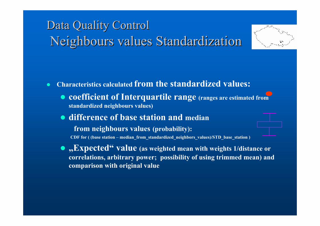
Data Data QQualityuality CControlontrolNeighbours values Neighbours values StandardizationStandardization

Characteristics calculated from the standardized values: coefficient of Interquartile range (ranges are estimated from standardized neighbours values)

difference of base station and median from neighbours values (probability):

CDF for ( (base station – median_from_standardized_neighbors_values)/STD_base_station )

„Expected“ value (as weighted mean with weights 1/distance orcorrelations, arbitrary power; possibility of using trimmed mean) and comparison with original value

QC, Settings in the softwareQC, Settings in the softwareprocessingprocessing thethe wholewhole datadatabasebase

2. Calculation:2. Calculation:1. Finding neighbours:1. Finding neighbours:

Example of outputs for outliers assessmentExample of outputs for outliers assessment

Altitudes

and distances of neighboursList of neighbours

Neighbour stations valuesExpected value

Suspicious values

Quality controlQuality control

Run for period 1961-2007, daily data (measured values in observation hours)All stations (200 climatological stations, 800 precipitation stations)All meteorological elements (T, TMA, TMI, TPM, SRA, SCE, SNO, E, RV, H, F) – parameters set individually

Historical records will follow now

Air temperature, Air temperature, number of outliers 1961number of outliers 1961--2007, 2007, from from 33..431431..000000 stationstation--daysdays

0

200

400

600

800

1000

1200

T_07:00 T_14:00 T_21:00 T_AVG TMA TMI TPM

T – air temperature at obs. hour, TMA – daily maximum temp., TMI – daily min. temp., TPM –daily ground minimum temp.

Air temperature, Air temperature, number of outliers 1961number of outliers 1961--2007, 2007, from from 33..431431..000000 stationstation--daysdays

Temperature

0

50

100

150

200

250

Jan Feb Mar Apr May Jun Jul Aug Sep Oct Nov Dec

07:00 14:00 21:00 AVG

Air temperature at obs. hour, AVG – daily average temp.

Air temperature, Air temperature, number of outliers 1961number of outliers 1961--2007, 2007,

Number of outliers per one station (all observation hours, AVG)

0.000

0.020

0.040

0.060

0.080

0.100

0.120

1961 1964 1967 1970 1973 1976 1979 1982 1985 1988 1991 1994 1997 2000 2003 2006

temperature

Water vapor pressure, Water vapor pressure, number of outliers 1961number of outliers 1961--2007, 2007, from from 33..431431..000000 stationstation--daysdays

Water vapor pressure at obs. hour, AVG – daily average

water vapour pressure

0

100

200

300

400

500

600

700

Jan Feb Mar Apr May Jun Jul Aug Sep Oct Nov Dec

07:00 14:00 21:00 AVG

Problematic detections Problematic detections -- heavy rainfallheavy rainfall

Problematic detections Problematic detections (heavy rainfall), Radar information(heavy rainfall), Radar information

Precipitation, Precipitation, number of outliers 1961number of outliers 1961--2007, 2007,

Number of outliers per one station

0.000

0.050

0.100

0.150

0.200

0.250

0.300

0.350

0.400

0.450

1961 1964 1967 1970 1973 1976 1979 1982 1985 1988 1991 1994 1997 2000 2003 2006

precipitation

Presented method can be further applied forPresented method can be further applied for

Filling missing values (the “expected” value)Calculation of technical series (e.g. for grid points -to be used for RCM validations or correction, EC FP6 project

CECILIA), …

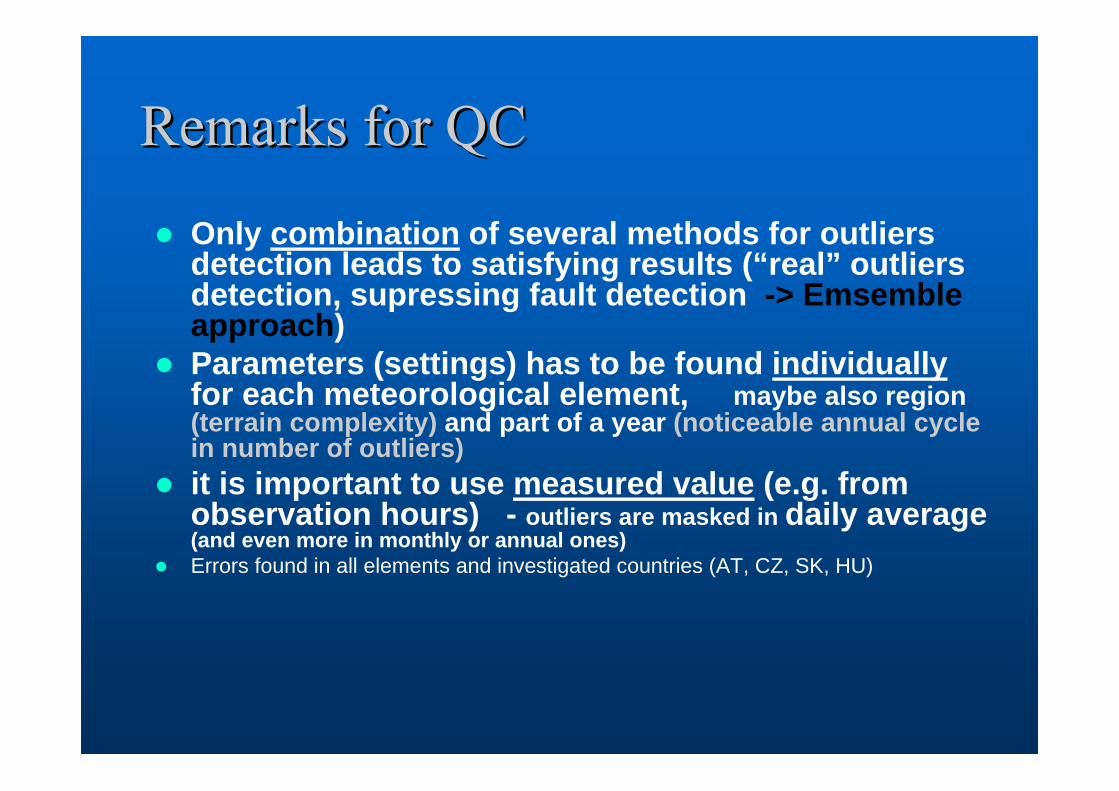
Remarks for QCRemarks for QC

Only combination of several methods for outliers detection leads to satisfying results (“real” outliers detection, supressing fault detection -> Emsembleapproach)Parameters (settings) has to be found individuallyfor each meteorological element, maybe also region (terrain complexity) and part of a year (noticeable annual cycle in number of outliers)it is important to use measured value (e.g. from observation hours) - outliers are masked in daily average (and even more in monthly or annual ones)Errors found in all elements and investigated countries (AT, CZ, SK, HU)

HomogenizationHomogenizationChange of measuring conditions

inhomogeneities

Data Processing

Interquartile Range Comparing to Neighbours

Alexandersson test Bivariate Test t-test Mann-Whitney-Pettit

from Correlations from Distances

Filling Miss. Values

Adjusting Data

Hom. Assessment

Reference Series

Homogeneity Testing

Combining Near Stations

Quality Control - Outliers

Monthly, Seasonal and Annual Averages

Several Iterations

Probability

Days, Months, seasons, year

How to increase number of test results How to increase number of test results (way to (way to automatizeautomatize -- objectiobjectifyfy inhomogeneities inhomogeneities detectiondetection phasephase))

for monthly, daily data (each month individually)

weighted/unweighted mean from neighbouring stationscriterions used for stations selection (or combination of it):– best correlated / nearest neighbours

(correlations – from the first differenced series)

– limit correlation, limit distance– limit difference in altitudes

neighbouring stations series should bestandardized to test series AVG and / or STD

(temperature - elevation, precipitation - variance)

- missing data are not so big problem then

CreatingCreating RReferenceeference SSerieseries

RelativeRelative homogeneityhomogeneity testingtesting

Available tests:– Alexandersson SNHT– Bivariate test of Maronna and Yohai– Mann – Whitney – Pettit test– t-test– Easterling and Peterson test– Vincent method– …

20 year parts of the daily series (40 for monthly series with 10 years overlap),

in SNHT splitting into subperiods in position of detected significant changepoint

(30-40 years per one inhomogeneity)

HomogeneityHomogeneity assessmentassessment

Various outputs created for betterinhomogeneities assessmentCombining results with information frommetadata whenever possible

Decision about „undoubted“ inhomogeneities (without metadata) – coincidence of test results


Test Ref I II III IV V VI VII VIII IX X XI XII Win Spr Sum Aut YearA avg 1927 1929 1927 1927 1927 1928 1927 1926 1926 1926 1926 1926 1927 1927 1927 1926 1927A 1930A corr 1927 1927 1927 1927 1927 1928 1927 1926 1926 1926 1926 1926 1927 1927 1927 1926 1927A 1939 1938 1939 1940 1922 1937 1937 1935A dist 1927 1928 1927 1927 1927 1928 1927 1926 1926 1926 1926 1926 1927 1927 1927 1926 1927A 1930 1940 1918B avg 1927 1928 1927 1927 1927 1928 1927 1926 1926 1926 1926 1926 1927 1927 1927 1926 1927B 1922B corr 1927 1927 1927 1927 1927 1928 1927 1926 1926 1926 1926 1926 1927 1927 1927 1926 1927B 1936 1938 1939 1944 1922 1935 1937 1937 1935B 1937B dist 1927 1928 1927 1927 1927 1928 1927 1926 1926 1926 1926 1926 1927 1927 1927 1926 1927B 1930 1940 1931 1913 1918V corr 1927 1926V 1937 1922 1935V 1937V dist 1927 1927 1927V 1918

Output example: Station Čáslav, 3rd segment, 1911-1950, n=40

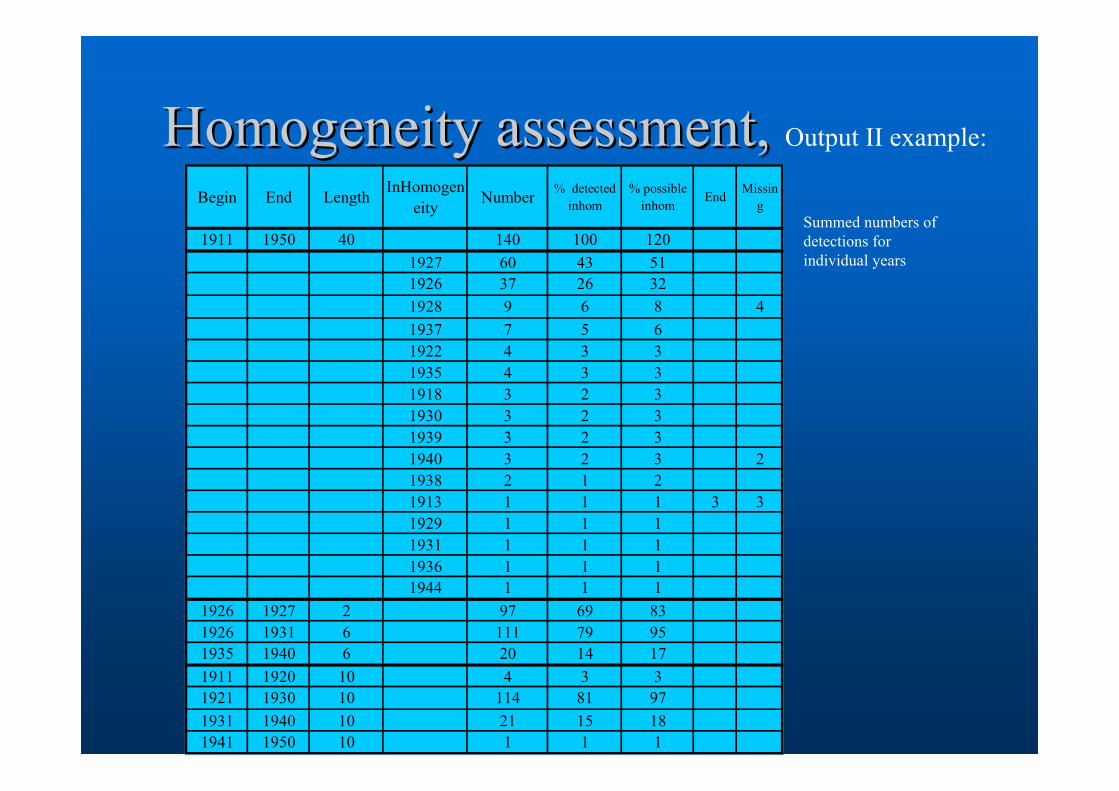
Begin End Length InHomogeneity Number % detected

inhom% possible

inhomEnd Missin

g

1911 1950 40 140 100 1201927 60 43 511926 37 26 321928 9 6 8 41937 7 5 61922 4 3 31935 4 3 31918 3 2 31930 3 2 31939 3 2 31940 3 2 3 21938 2 1 21913 1 1 1 3 31929 1 1 11931 1 1 11936 1 1 11944 1 1 1

1926 1927 2 97 69 831926 1931 6 111 79 951935 1940 6 20 14 171911 1920 10 4 3 31921 1930 10 114 81 971931 1940 10 21 15 181941 1950 10 1 1 1

HomogeneityHomogeneity assessmentassessment, , Output II example:

Summed numbers ofdetections for individual years


ID ELYEAR_BEGINEND YEAR_COUNY_POSSIBL YEAMIS X_BEGIN_DX_END_DATX_X_L L ABREMARKC C_x B1BOJK01 x 1985 41 14.24 12 23.3.1984 31.3.2003 # # Bchange

B1BOJK01 x 1985 41 14.24 12 23.3.1984 31.12.9999 # # obs V BB1BYSH01 x 1978 37 12.85

? B1BYSH01 x 1979 33 11.46? B1BYSH01 x 1980 43 14.93? B1HLHO01 x 1965 31 10.76 4 1

B1HOLE01 x 1976 33 11.46B1KROM01 x 1977 1978 31 10.76

x B1RADE01 x 1994 44 15.28 2 1.1.1994 31.12.9999 # # RchangeB1RADE01 x 1994 44 15.28 2 1.1.1994 31.12.9999 # # obs JoB

x B1RYCH01 x 1973 49 17.01 1.5.1973 28.2.1991 # # VchangeB1RYCH01 x 1973 49 17.01 1.9.1972 28.2.1991 # # obs MB

xx? B1STRZ01 x 1987 53 18.40B1STRZ01 x 1988 30 10.42B1UHBR01 x 1983 31 10.76 18.2.1984 31.1.1999 # # UchangeB1UHBR01 x 1983 31 10.76 18.2.1984 12.5.1993 # # obs JoB

x B1UHBR01 x 1984 77 26.74 18.2.1984 31.1.1999 # # UchangeB1UHBR01 x 1984 77 26.74 18.2.1984 12.5.1993 # # obs JoBB1VELI01 x 1978 31 10.76

? B1VELI01 x 1977 1978 44 15.28? B1VKLO01 x 1984 29 10.07x B1VYSK01 x 1999 32 11.11 -1 1.4.1998 31.12.9999 # # Vchange

B1VYSK01 x 1999 32 11.11 -1 1.4.1998 31.12.9999 # # obs V BB2BOSK01_rx 1968 33 11.46B2BREC01 x 1968 35 12.15B2BRUM01 x 1989 51 17.71 1.2.1989 31.3.1994 # # BchangeB2BRUM01 x 1989 51 17.71 1.2.1989 31.3.1994 # # obs MB

-1 .0

-0 .8

-0 .6

-0 .4

-0 .2

0.0

0.2

0.4

0.6

0.8

1911 1915 1919 1923 1927 1931 1935 1939 1943 1947

combining several outputs (sums of detections in individual years, metadata, graphs of differences/ratios, …)

Inhomogeneities Inhomogeneities detectiondetection andandcorrectioncorrection

Detection – for months, seasons, yearCorrection – daily, for each months separately

AdjustAdjustinging dailydaily valuesvalues for inhomogeneitiesfor inhomogeneities, ,

„delta“ methodinterpolation of monthly factors– MASH– Vincent et al (2002)

Is it natural that station changes has the same effect upon low and high extremes …?

Variable correctionE.g.– Higher Order Moments (HOM), by Della Marta and

Wanner (2006)– Two phase non-linear regression by Mestre

(SPLIDHOM)– our own percentile approach (similar to Déqué…….)

AdjustAdjustinging dailydaily valuesvalues forfor inhomogeneitiesinhomogeneities, ,

VariableVariable correctioncorrection, The higher-order moments method

DELLA-MARTA AND WANNER,

JOURNAL OF CLIMATE 19 (2006) 4179-4197

VariableVariable correctioncorrection

1996

Iterative homogeneity testingIterative homogeneity testing

several iteration of testing and results evaluation– several iterations of homogeneity testing and

series adjusting (3 iterations should be sufficient)

– question of homogeneity of reference series isthus solved:

• possible inhomogeneities should be eliminated by using averages of several neighbouring stations

• if this is not true: in next iteration neighbours shouldbe already homogenized

FillingFilling missingmissing valuesvaluesBefore homogenization: influence on right inhomogeneity detectionAfter homogenization: more precise - data are not influenced by possible shifts in the series

Dependence of tested series on reference series

#

#

Prague

Brno

HomogenizationHomogenizationofof thethe seriesseries in in the Czech Republicthe Czech Republic

NumberNumber ofof inhomogeneities inhomogeneities explainedexplained by by metadatametadata

0

20

40

60

80

100

120

140

160

180

200

T_AVG TMA TMI SRA SSV E F

Coun

t

metada no metada

T – air temperature, TMA – maximum temperature, TMI – minimum temperature, SRA – precipitation, SSV – sunshine duration, E – water vapour pressure, F – windspeed

NumberNumber ofof inhomogeneities inhomogeneities explainedexplained by by metadatametadata, T_AVG, T_AVG

0

2

4

6

8

10

1219

61

1963

1965

1967

1969

1971

1973

1975

1977

1979

1981

1983

1985

1987

1989

1991

1993

1995

1997

1999

2001

2003

2005

2007

Coun

t

no metadata

metadata

metadata - AMS

0

1

2

3

4

5

6

7

8

9

10

1961

1964

1967

1970

1973

1976

1979

1982

1985

1988

1991

1994

1997

2000

2003

2006

Coun

t

no metadata

metadata

0

1

2

3

4

5

6

7

8

9

10

1961

1964

1967

1970

1973

1976

1979

1982

1985

1988

1991

1994

1997

2000

2003

2006

Coun

t

no metadata

metadata

Tmax

Tmin

HomogeneityHomogeneity testingtesting resultsresultsAirAir temperaturetemperature

Number of detected inhomogeneities (significant, 0.05)

0

50

100

150

200

250

300

350

400

450

Jan Feb Mar Apr May Jun Jul Aug Sep Oct Now Dec0

50

100

150

200

250

300

350

400

450

Year DJF MAM JJA SON

Correlations between tested and reference series, daily valuesAir temperature

Boxplots:

- Median, average

- Upper and lower quartiles

- minimum and maximum value

(for 115 stations)

0.80

0.82

0.84

0.86

0.88

0.90

0.92

0.94

0.96

0.98

1.00

Jan Feb Mar Apr May Jun Jul Aug Sep Oct Nov Dec0.80

0.82

0.84

0.86

0.88

0.90

0.92

0.94

0.96

0.98

1.00


Adjustments, monthly averages of abs. valuesAir temperature

Boxplots:

- Median, average



(for 115 stations)

0.00

0.20

0.40

0.60

0.80

1.00

1.20

1.40

1.60


0.20

0.40

0.60

0.80

1.00

1.20

1.40

1.60


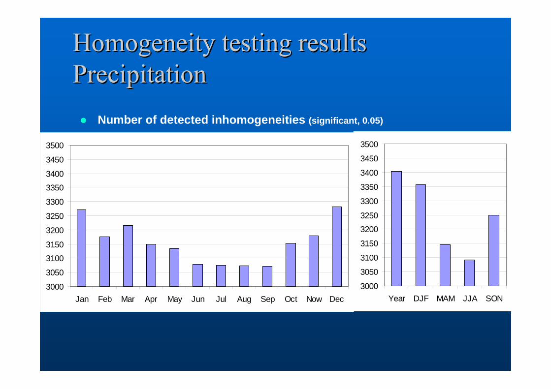
HomogeneityHomogeneity testingtesting resultsresultsPrecipitationPrecipitation

Number of detected inhomogeneities (significant, 0.05)

3000

3050

31003150

3200

3250

3300

33503400

3450

3500

Jan Feb Mar Apr May Jun Jul Aug Sep Oct Now Dec3000

3050

3100

3150

32003250

3300

3350

3400

3450

3500


Correlations between tested and reference series, daily valuesPrecipitation

Boxplots:- Median, average- Upper and lower quartiles- minimum and maximum value(for 121 stations)

0.00

0.10

0.20

0.30

0.40

0.50

0.60

0.70

0.80

0.90

1.00


0.10

0.20

0.30

0.40

0.50

0.60

0.70

0.80

0.90

1.00

Year DJF MAM JJA SON0.50

0.55

0.60

0.65

0.70

0.75

0.80

0.85

0.90

0.95

1.00


0.55

0.60

0.65

0.70

0.75

0.80

0.85

0.90

0.95

1.00


Adjustments, monthly averages of quotines < 1Precipitation

Boxplots:

- Median, average



(for 115 stations)

0.00

0.20

0.40

0.60

0.80

1.00

1.20

1.40

1.60

1.80

2.00


0.10

0.20

0.30

0.40

0.50

0.60

0.70

0.80

0.90

1.00


Change of measuring conditions at the station (relocation etc.) is manifested in the series mainly in summer

in winter: active surface role is diminished, prevailing circulation factors, in summer: active surface role increases, prevailing radiation factors

Inhomogeneities Inhomogeneities in summer versus in winterin summer versus in winter,,AirAir temperaturetemperature

Inhomogeneities Inhomogeneities in summer versus in winterin summer versus in winter,,PrecipitationPrecipitation

Change of measuring conditions at the station (relocation etc.) is manifested in the series mainly in winter

in winter: errors of measurement (solid precipitation - wind, …)

HomogenizationHomogenizationConlusionsConlusions

- „Ensemble“ approach to homogenization (combining information from different statistical tests, time frames, overlapping periods, reference series, meteorological elements, …) - more information for inhomogeneities assessment – higher quality of homogenization in case metadata are incompleteannual cycle of inhomogeneities, adjustments, …

Software Software usedused for data for data processingprocessing

LoadData - application for downloading data fromcentral database (e.g. Oracle)

ProClimDB software for processing wholedataset (finding outliers, combining series, creatingreference series, preparing data for homogeneity testing, extreme value analysis, RCM outputs validation, correction, …)

AnClim software for homogeneity testing

http://www.http://www.cclimahomlimahom..eueu

AnClim softwareAnClim software

AnClim softwareAnClim software

ProcDataProcData softwaresoftware

ProProClimDBClimDB softwaresoftware

http://www.http://www.cclimahomlimahom..eueu

data quality control and homogenization of air temperature ... · data quality control finding...

Documents