Data Preprocessing

Data Preprocessing

Why preprocess the data?

Data cleaning

Data integration and transformation

Data reduction

Discretization and concept hierarchy

generation

Summary

Why Data Preprocessing?

Data in the real world is dirty incomplete: lacking attribute values, lacking certain

attributes of interest, or containing only aggregate data noisy: containing errors or outliers inconsistent: containing discrepancies in codes or

names No quality data, no quality mining results!

Quality decisions must be based on quality data Data warehouse needs consistent integration of quality

data Required for both OLAP and Data Mining!

Why can Data be Incomplete?

Attributes of interest are not available (e.g., customer information for sales transaction data)

Data were not considered important at the time of transactions, so they were not recorded!

Data not recorder because of misunderstanding or malfunctions

Data may have been recorded and later deleted! Missing/unknown values for some data

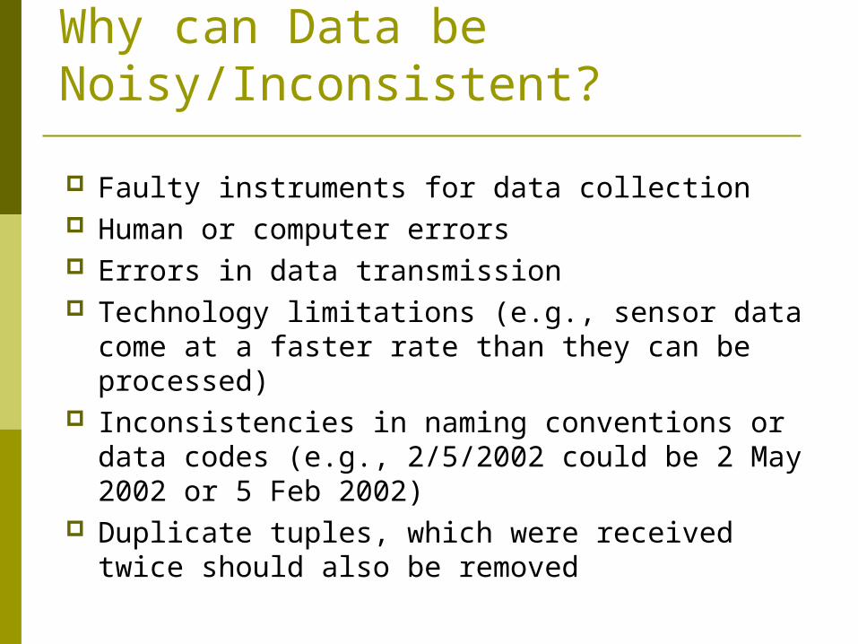
Why can Data be Noisy/Inconsistent?

Faulty instruments for data collection Human or computer errors Errors in data transmission Technology limitations (e.g., sensor data come at

a faster rate than they can be processed) Inconsistencies in naming conventions or data

codes (e.g., 2/5/2002 could be 2 May 2002 or 5 Feb 2002)

Duplicate tuples, which were received twice should also be removed

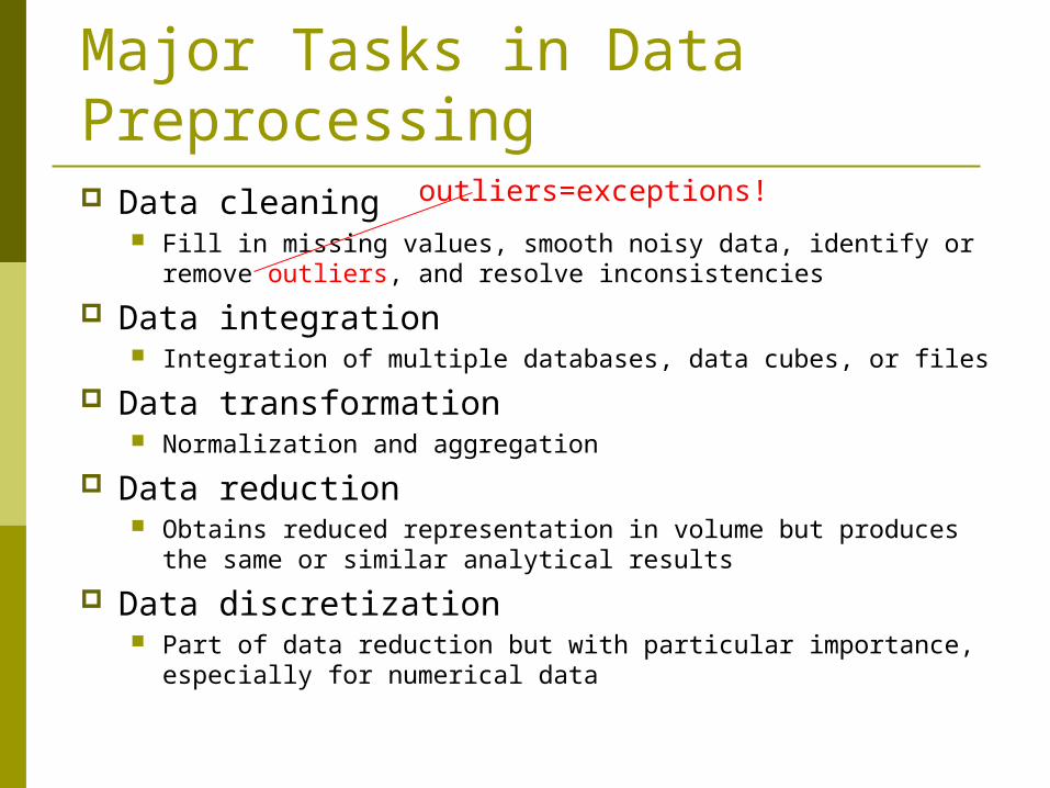
Major Tasks in Data Preprocessing Data cleaning

Fill in missing values, smooth noisy data, identify or remove outliers, and resolve inconsistencies

Data integration Integration of multiple databases, data cubes, or files

Data transformation Normalization and aggregation

Data reduction Obtains reduced representation in volume but produces the

same or similar analytical results

Data discretization Part of data reduction but with particular importance,

especially for numerical data

outliers=exceptions!

Forms of data preprocessing

Data Preprocessing

Why preprocess the data?

Data cleaning

Data integration and transformation

Data reduction

Discretization and concept hierarchy

generation

Summary

Data Cleaning

Data cleaning tasks

Fill in missing values

Identify outliers and smooth out noisy data

Correct inconsistent data

How to Handle Missing Data?

Ignore the tuple: usually done when class label is missing

(assuming the tasks in classification)—not effective when the

percentage of missing values per attribute varies considerably.

Fill in the missing value manually: tedious + infeasible?

Use a global constant to fill in the missing value: e.g.,

“unknown”, a new class?!

Use the attribute mean to fill in the missing value

Use the attribute mean for all samples belonging to the same

class to fill in the missing value: smarter

Use the most probable value to fill in the missing value:

inference-based such as Bayesian formula or decision tree

How to Handle Missing Data?

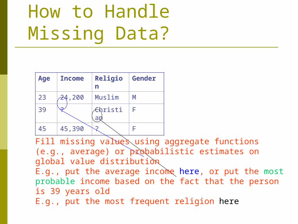
Age Income Religion Gender

23 24,200 Muslim M

39 ? Christian F

45 45,390 ? F

Fill missing values using aggregate functions (e.g., average) or probabilistic estimates on global value distributionE.g., put the average income here, or put the most probable income based on the fact that the person is 39 years oldE.g., put the most frequent religion here

Noisy Data

Noise: random error or variance in a measured variable

Incorrect attribute values may exist due to faulty data collection instruments data entry problems data transmission problems technology limitation inconsistency in naming convention

Other data problems which requires data cleaning duplicate records incomplete data inconsistent data

How to Handle Noisy Data?Smoothing techniques

Binning method: first sort data and partition into (equi-depth) bins then one can smooth by bin means, smooth by bin

median, smooth by bin boundaries, etc. Clustering

detect and remove outliers Combined computer and human inspection

computer detects suspicious values, which are then checked by humans

Regression smooth by fitting the data into regression functions

Use Concept hierarchies use concept hierarchies, e.g., price value -> “expensive”

Simple Discretization Methods: Binning

Equal-width (distance) partitioning: It divides the range into N intervals of equal size:

uniform grid if A and B are the lowest and highest values of the

attribute, the width of intervals will be: W = (B-A)/N. The most straightforward But outliers may dominate presentation Skewed data is not handled well.

Equal-depth (frequency) partitioning: It divides the range into N intervals, each containing

approximately same number of samples Good data scaling – good handing of skewed data

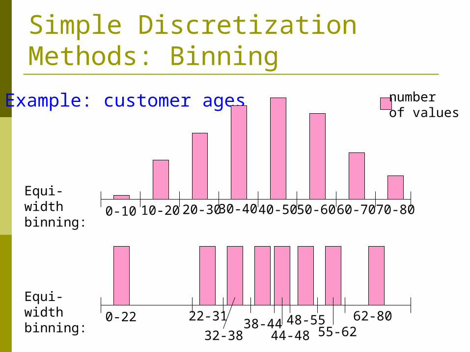
Simple Discretization Methods: Binning

Example: customer ages

0-10 10-20 20-30 30-40 40-50 50-60 60-70 70-80

Equi-width binning:

numberof values

0-22 22-31

44-4832-3838-44 48-55

55-6262-80

Equi-width binning:

Smoothing using Binning Methods

* Sorted data for price (in dollars): 4, 8, 9, 15, 21, 21, 24, 25, 26, 28, 29, 34

* Partition into (equi-depth) bins: - Bin 1: 4, 8, 9, 15 - Bin 2: 21, 21, 24, 25 - Bin 3: 26, 28, 29, 34* Smoothing by bin means: - Bin 1: 9, 9, 9, 9 - Bin 2: 23, 23, 23, 23 - Bin 3: 29, 29, 29, 29* Smoothing by bin boundaries: [4,15],[21,25],[26,34] - Bin 1: 4, 4, 4, 15 - Bin 2: 21, 21, 25, 25 - Bin 3: 26, 26, 26, 34

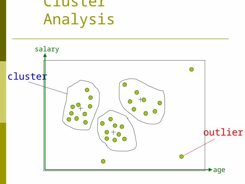
Cluster Analysis

cluster

outlier

salary

age

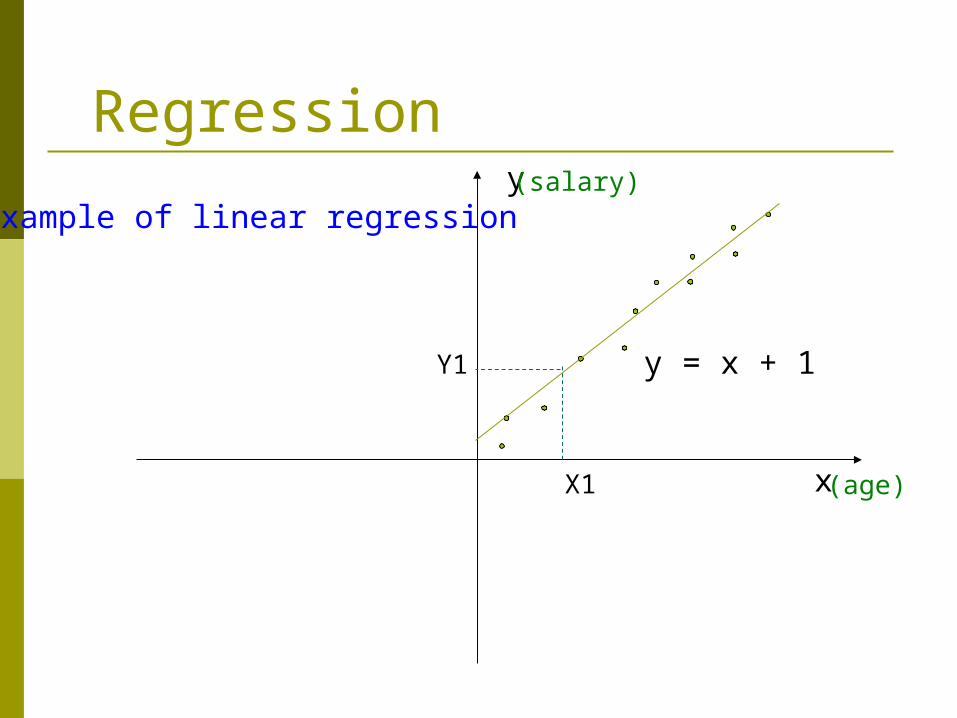
Regression

x

y

y = x + 1

X1

Y1

(salary)

(age)

Example of linear regression

Inconsistent Data Inconsistent data are handled by:

Manual correction (expensive and tedious) Use routines designed to detect inconsistencies

and manually correct them. E.g., the routine may use the check global constraints (age>10) or functional dependencies

Other inconsistencies (e.g., between names of the same attribute) can be corrected during the data integration process

Data Preprocessing

Why preprocess the data?

Data cleaning

Data integration and transformation

Data reduction

Discretization and concept hierarchy

generation

Summary

Data Integration

Data integration: combines data from multiple sources into a coherent store

Schema integration integrate metadata from different sources

metadata: data about the data (i.e., data descriptors) Entity identification problem: identify real world entities

from multiple data sources, e.g., A.cust-id B.cust-# Detecting and resolving data value conflicts

for the same real world entity, attribute values from different sources are different (e.g., J.D.Smith and Jonh Smith may refer to the same person)

possible reasons: different representations, different scales, e.g., metric vs. British units (inches vs. cm)

Handling Redundant Data in Data Integration

Redundant data occur often when integration of multiple databases The same attribute may have different names in different

databases One attribute may be a “derived” attribute in another

table, e.g., annual revenue

Redundant data may be able to be detected by correlation analysis

Careful integration of the data from multiple sources may help reduce/avoid redundancies and inconsistencies and improve mining speed and quality

Data Transformation

Smoothing: remove noise from data Aggregation: summarization, data cube

construction Generalization: concept hierarchy climbing Normalization: scaled to fall within a small,

specified range min-max normalization z-score normalization normalization by decimal scaling

Attribute/feature construction New attributes constructed from the given ones

Normalization: Why normalization? Speeds-up some learning techniques (ex.

neural networks) Helps prevent attributes with large

ranges outweigh ones with small ranges Example:

income has range 3000-200000 age has range 10-80 gender has domain M/F

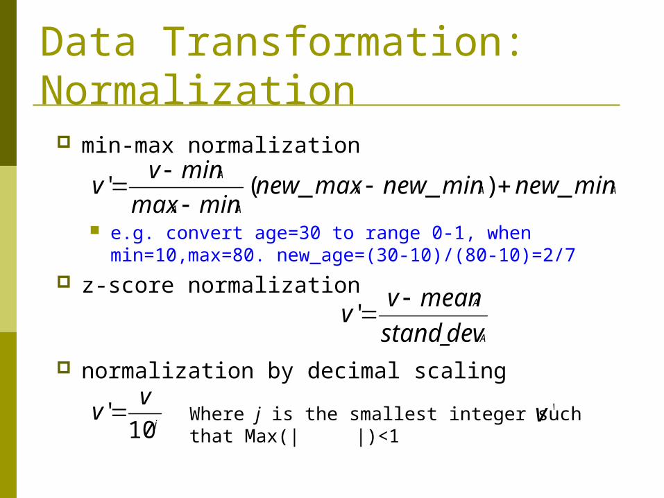
Data Transformation: Normalization

min-max normalization

e.g. convert age=30 to range 0-1, when min=10,max=80. new_age=(30-10)/(80-10)=2/7

z-score normalization

normalization by decimal scaling

AAA

AA

A

minnewminnewmaxnewminmax

minvv _)__('

A

A

devstand_

meanvv

'

j

vv

10' Where j is the smallest integer such that Max(| |)<1'v

Data Preprocessing

Why preprocess the data?

Data cleaning

Data integration and transformation

Data reduction

Discretization and concept hierarchy

generation

Summary

Data Reduction Strategies

Warehouse may store terabytes of data: Complex data analysis/mining may take a very long time to run on the complete data set

Data reduction Obtains a reduced representation of the data set that is

much smaller in volume but yet produces the same (or almost the same) analytical results

Data reduction strategies Data cube aggregation Dimensionality reduction Data compression Numerosity reduction Discretization and concept hierarchy generation

Data Cube Aggregation

The lowest level of a data cube the aggregated data for an individual entity of interest

e.g., a customer in a phone calling data warehouse.

Multiple levels of aggregation in data cubes Further reduce the size of data to deal with

Reference appropriate levels Use the smallest representation which is enough to solve

the task

Queries regarding aggregated information should be answered using data cube, when possible

Dimensionality Reduction

Feature selection (i.e., attribute subset selection): Select a minimum set of features such that the probability

distribution of different classes given the values for those features is as close as possible to the original distribution given the values of all features

reduce # of patterns in the patterns, easier to understand Heuristic methods (due to exponential # of choices):

step-wise forward selection step-wise backward elimination combining forward selection and backward elimination decision-tree induction

Heuristic Feature Selection Methods

There are 2d possible sub-features of d features Several heuristic feature selection methods:

Best single features under the feature independence assumption: choose by significance tests.

Best step-wise feature selection: The best single-feature is picked first Then next best feature condition to the first, ...

Step-wise feature elimination: Repeatedly eliminate the worst feature

Best combined feature selection and elimination: Optimal branch and bound:

Use feature elimination and backtracking

Example of Decision Tree Induction

Initial attribute set:{A1, A2, A3, A4, A5, A6}

A4 ?

A1? A6?

Class 1 Class 2 Class 1 Class 2

> Reduced attribute set: {A1, A4, A6}

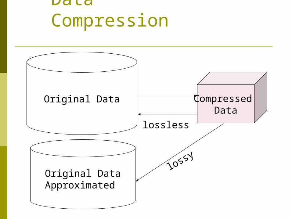
Data Compression

Original Data Compressed Data

lossless

Original DataApproximated

lossy

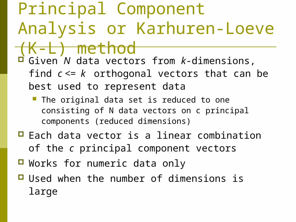
Given N data vectors from k-dimensions, find c <= k orthogonal vectors that can be best used to represent data The original data set is reduced to one consisting of N

data vectors on c principal components (reduced dimensions)

Each data vector is a linear combination of the c principal component vectors

Works for numeric data only Used when the number of dimensions is large

Principal Component Analysis or Karhuren-Loeve (K-L) method

X1

X2

Y1

Y2

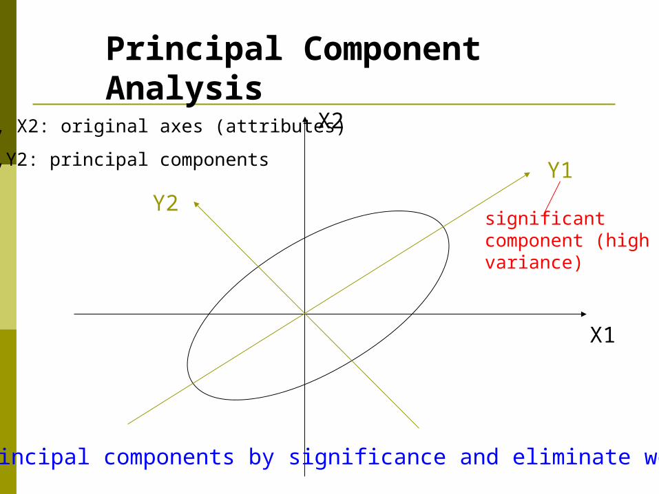
Principal Component Analysis

X1, X2: original axes (attributes)

Y1,Y2: principal components

significant component (high variance)

Order principal components by significance and eliminate weaker ones

Numerosity Reduction:Reduce the volume of data

Parametric methods Assume the data fits some model, estimate model

parameters, store only the parameters, and discard the data (except possible outliers)

Log-linear models: obtain value at a point in m-D space as the product on appropriate marginal subspaces

Non-parametric methods Do not assume models Major families: histograms, clustering, sampling

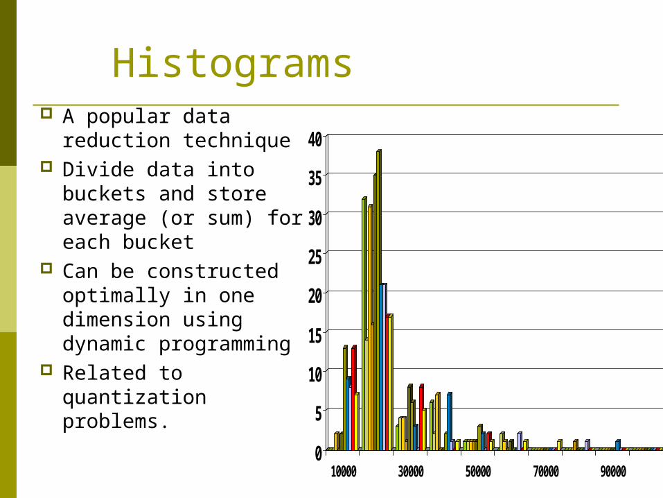
Histograms A popular data

reduction technique Divide data into buckets

and store average (or sum) for each bucket

Can be constructed optimally in one dimension using dynamic programming

Related to quantization problems.

0

5

10

15

20

25

30

35

40

10000 30000 50000 70000 90000

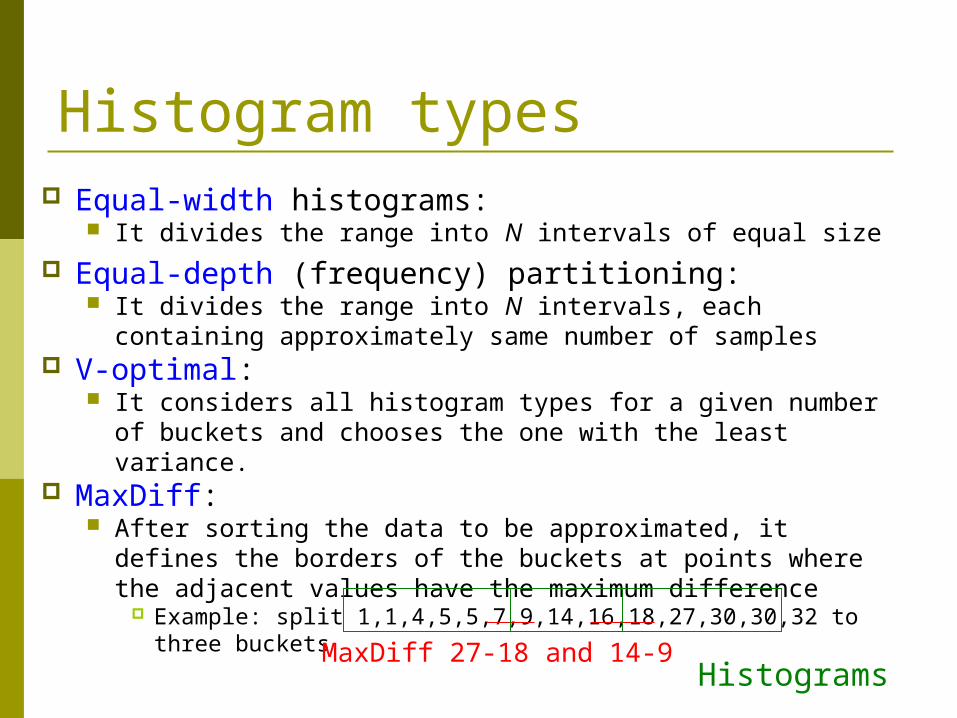
Histogram types Equal-width histograms:

It divides the range into N intervals of equal size Equal-depth (frequency) partitioning:

It divides the range into N intervals, each containing approximately same number of samples

V-optimal: It considers all histogram types for a given number of

buckets and chooses the one with the least variance. MaxDiff:

After sorting the data to be approximated, it defines the borders of the buckets at points where the adjacent values have the maximum difference

Example: split 1,1,4,5,5,7,9,14,16,18,27,30,30,32 to three buckets MaxDiff 27-18 and 14-9

Histograms

Clustering

Partitions data set into clusters, and models it by

one representative from each cluster

Can be very effective if data is clustered but not

if data is “smeared”

There are many choices of clustering definitions

and clustering algorithms, further detailed in

Chapter 7

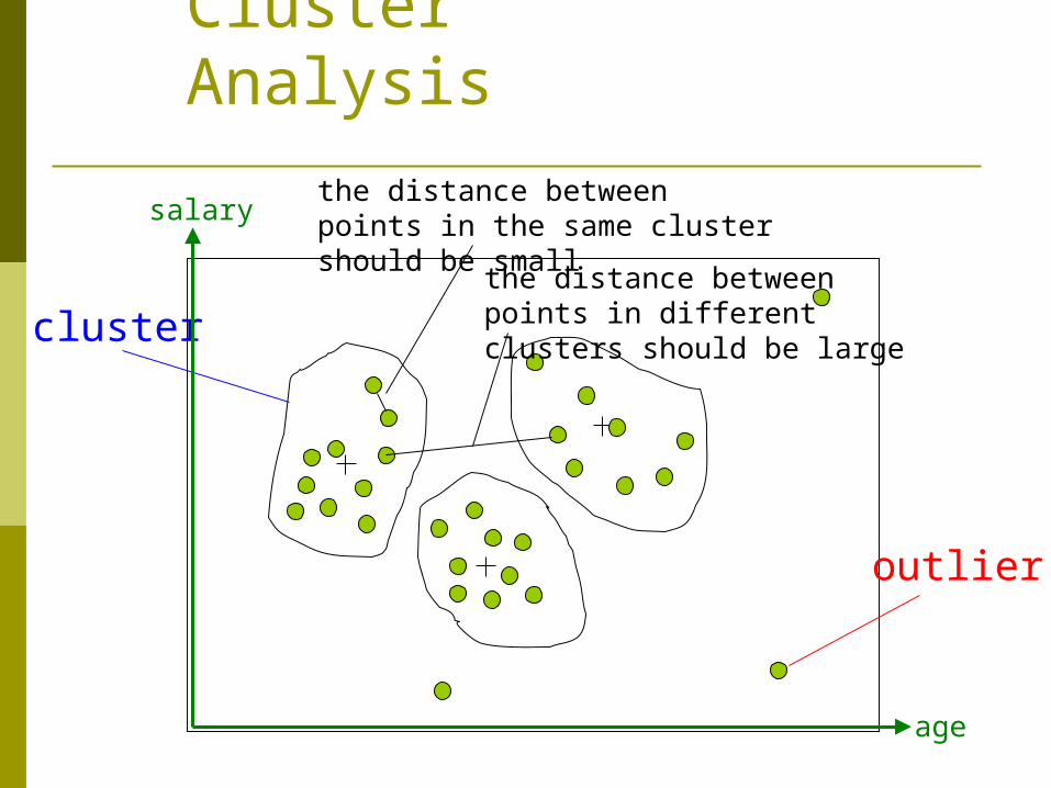
Cluster Analysis

cluster

outlier

salary

age

the distance between points in the same cluster should be small

the distance between points in different clusters should be large

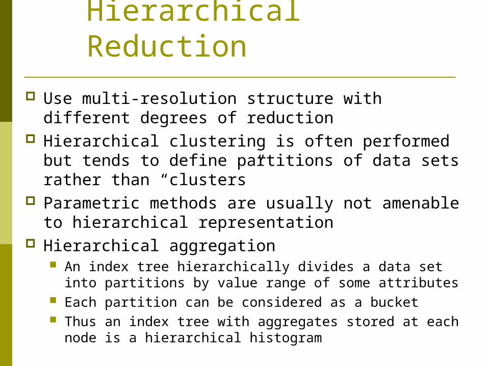
Hierarchical Reduction

Use multi-resolution structure with different degrees of reduction

Hierarchical clustering is often performed but tends to define partitions of data sets rather than “clusters”

Parametric methods are usually not amenable to hierarchical representation

Hierarchical aggregation An index tree hierarchically divides a data set into

partitions by value range of some attributes Each partition can be considered as a bucket Thus an index tree with aggregates stored at each node is

a hierarchical histogram

Data Preprocessing

Why preprocess the data?

Data cleaning

Data integration and transformation

Data reduction

Discretization and concept hierarchy

generation

Summary

Discretization Three types of attributes:

Nominal — values from an unordered set Ordinal — values from an ordered set Continuous — real numbers

Discretization: divide the range of a continuous attribute into

intervals why?

Some classification algorithms only accept categorical attributes.

Reduce data size by discretization Prepare for further analysis

Discretization and Concept hierachy

Discretization reduce the number of values for a given continuous

attribute by dividing the range of the attribute into intervals. Interval labels can then be used to replace actual data values.

Concept hierarchies reduce the data by collecting and replacing low level

concepts (such as numeric values for the attribute age) by higher level concepts (such as young, middle-aged, or senior).

Discretization and concept hierarchy generation for numeric data

Binning/Smoothing (see sections before)

Histogram analysis (see sections before)

Clustering analysis (see sections before)

Entropy-based discretization

Segmentation by natural partitioning

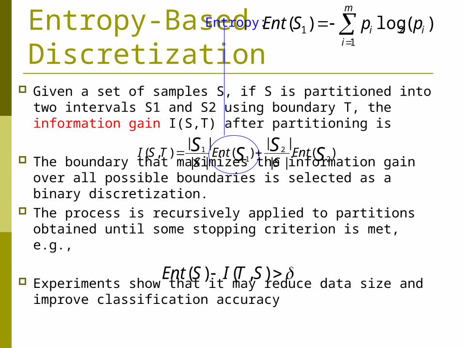
Entropy-Based Discretization

Given a set of samples S, if S is partitioned into two intervals S1 and S2 using boundary T, the information gain I(S,T) after partitioning is

The boundary that maximizes the information gain over all possible boundaries is selected as a binary discretization.

The process is recursively applied to partitions obtained until some stopping criterion is met, e.g.,

Experiments show that it may reduce data size and improve classification accuracy

)(||

||)(

||

||),(

22

11 SSSS Ent

SEnt

STSI

),()( STISEnt

)(log)( 21

1 i

m

ii ppSEnt

Entropy:

Segmentation by natural partitioning

The 3-4-5 rule can be used to segment numerical data into

relatively uniform, “natural” intervals.

* If an interval covers 3, 6, 7 or 9 distinct values at the most significant digit, partition the range into 3 equiwidth intervals for 3,6,9 or 2-3-2 for 7

* If it covers 2, 4, or 8 distinct values at the most significant digit, partition the range into 4 equiwidth intervals

* If it covers 1, 5, or 10 distinct values at the most significant digit, partition the range into 5 equiwidth intervals

Users often like to see numerical ranges partitioned into relatively uniform, easy-to-read intervals that appear intuitive or “natural”. E.g., [50-60] better than [51.223-60.812]

The rule can be recursively applied for the resulting intervals

Concept hierarchy generation for categorical data Categorical attributes: finite, possibly large domain, with no

ordering among the values Example: item type

Specification of a partial ordering of attributes explicitly at the schema level by users or experts Example: location is split by domain experts to

street<city<state<country

Specification of a portion of a hierarchy by explicit data

grouping

Specification of a set of attributes, but not of their partial

ordering

Specification of only a partial set of attributes

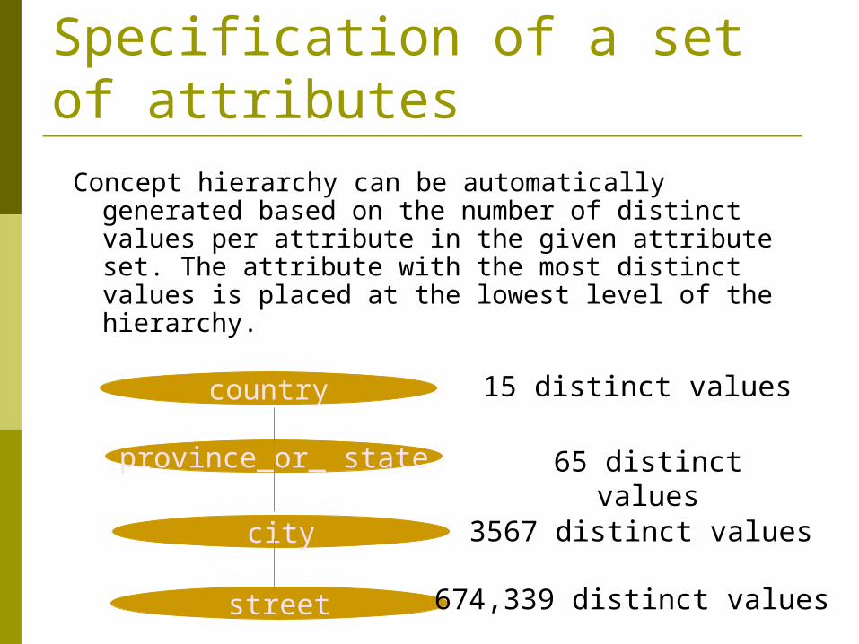
Specification of a set of attributes

Concept hierarchy can be automatically generated based on the number of distinct values per attribute in the given attribute set. The attribute with the most distinct values is placed at the lowest level of the hierarchy.

country

province_or_ state

city

street

15 distinct values

65 distinct values

3567 distinct values

674,339 distinct values