data parallelism - computer science · • data parallelism • using opencl to create ... allows...

© Kenneth M. Anderson, 2016

Data Parallelism

CSCI 5828: Foundations of Software EngineeringLecture 28 — 12/01/2016

1


Goals

• Cover the material in Chapter 7 of Seven Concurrency Models in Seven Weeks by Paul Butcher

• Data Parallelism

• Using OpenCL to create parallel programs on the GPU

• Also look at two examples that use OpenCL and OpenGL together

2

Prepared exclusively for Ken Anderson


Data Parallelism

• Data Parallelism is an approach to concurrent programming that can perform number crunching on a computer’s GPU

• You typically create a bunch of arrays and load them onto the GPU

• You also create a “kernel”; a program that is loaded onto the GPU

• The kernel then applies the operations of its program to the elements of the array in parallel.

• So, if you had two arrays of 1024 floating point numbers and you wanted to multiply those arrays together, the GPU might be able to perform that multiplication on all 1024 pairs “at once”

• In actuality, the kernel is transformed into a program for your particular GPU that makes use of pipelining and multiple ALUs to process the operation as efficiently as possible

3


Pipelining (I)

• One way that data parallelism can be implemented is via pipelining

• int result = 13 * 2;

• We might think of the above multiplication as an atomic operation

• but on the CPU, at the level of “gates”, it takes several steps

• Those steps are typically arranged as a pipeline

• In this example, if each step takes one clock cycle, it would take 5 clock cycles to perform the multiplication

4

Day 1: GPGPU ProgrammingToday we’ll see how to create a simple GPGPU program that multiplies twoarrays in parallel, and then we’ll benchmark it to see just how much fasterthe GPU is than the CPU. First, though, we’ll spend a little time examiningwhat makes a GPU so powerful when it comes to number-crunching.

Graphics Processing and Data ParallelismComputer graphics is all about manipulating data—huge amounts of data.And doing it quickly. A scene in a 3D game is constructed from a myriad oftiny triangles, each of which needs to have its position on the screen calculatedin perspective relative to the viewpoint, clipped, lit, and textured twenty-fiveor more times a second.

The great thing about this is that although the amount of data that needs tobe processed is huge, the actual operations on that data are relatively simplevector or matrix operations. This makes them very amenable to data paral-lelization, in which multiple computing units perform the same operationson different items of data in parallel.

Modern GPUs are exceptionally sophisticated, powerful parallel processorscapable of rendering billions of triangles a second. The good news is thatalthough they were originally designed with graphics alone in mind, theircapabilities have evolved to the point that they’re useful for a much widerrange of applications.

Data parallelism can be implemented in many different ways. We’ll look brieflyat a couple of them: pipelining and multiple ALUs.

Pipelining

Although we tend to think of multiplying two numbers as a single atomicoperation, down at the level of the gates on a chip, it actually takes severalsteps. These steps are typically arranged as a pipeline:

Operand 1

Operand 2

Result

For the five-element pipeline shown here, if it takes a single clock cycle foreach step to complete, multiplying a pair of numbers will take five clock cycles.But if we have lots of numbers to multiply, things get much better because(assuming our memory subsystem can supply the data fast enough) we cankeep the pipeline full:

Chapter 7. Data Parallelism • 190

report erratum • discussPrepared exclusively for Ken Anderson


Pipelining (II)

• If we only sent two numbers to this pipeline, our code would be inefficient

• Instead, if we have lots of numbers to multiply, we can insert new numbers to multiply at the start of the pipeline for each new clock cycle

• Here, arrays A and B are being multiplied and we’re inserting one new element of each array into the start of the pipeline, each clock cycle• 1000 numbers would take ~1000 clock cycles to multiply (rather than

5000)!

5

a7*b7 a6*b6 a5*b5 a4*b4 a3*b3

a1*b1 a2*b2b8b7b6 b9

a8a7a6 a9

So multiplying a thousand pairs of numbers takes a whisker over a thousandclock cycles, not the five thousand we might expect from the fact that multi-plying a single pair takes five clock cycles.

Multiple ALUs

The component within a CPU that performs operations such as multiplicationis commonly known as the arithmetic logic unit, or ALU:

Operand 1 Operand 2

Result

Couple multiple ALUs with a wide memory bus that allows multiple operandsto be fetched simultaneously, and operations on large amounts of data canagain be parallelized, as shown in Figure 12, Large Amounts of Data Paral-lelized with Multiple ALUs, on page 192.

GPUs typically have a 256-bit or wider memory bus, allowing (for example)eight or more 32-bit floating-point numbers to be fetched at a time.

A Confused Picture

To achieve their performance, real-world GPUs combine pipelining and multipleALUs with a wide range of other techniques that we’ll not cover here. By itself,this would make understanding the details of a single GPU complex. Unfortu-nately, there’s little commonality between different GPUs (even those producedby a single manufacturer). If we had to write code that directly targeted aparticular architecture, GPGPU programming would be a nonstarter.

OpenCL targets multiple architectures by defining a C-like language thatallows us to express a parallel algorithm abstractly. Each different GPU

report erratum • discuss

Day 1: GPGPU Programming • 191



ALUs (I)

• Arithmetic logic units (ALUs) perform computations for CPUs

• They take two inputs and perform a result

• Another way to perform parallel operations on a GPU is to:

• create a series of linked ALUs that compute a result

• and combine it with a “wide bus” that allows multiple operands to be fetched at the same time

6

a7*b7 a6*b6 a5*b5 a4*b4 a3*b3

a1*b1 a2*b2b8b7b6 b9

a8a7a6 a9

So multiplying a thousand pairs of numbers takes a whisker over a thousandclock cycles, not the five thousand we might expect from the fact that multi-plying a single pair takes five clock cycles.

Multiple ALUs

The component within a CPU that performs operations such as multiplicationis commonly known as the arithmetic logic unit, or ALU:

Operand 1 Operand 2

Result

Couple multiple ALUs with a wide memory bus that allows multiple operandsto be fetched simultaneously, and operations on large amounts of data canagain be parallelized, as shown in Figure 12, Large Amounts of Data Paral-lelized with Multiple ALUs, on page 192.

GPUs typically have a 256-bit or wider memory bus, allowing (for example)eight or more 32-bit floating-point numbers to be fetched at a time.

A Confused Picture

To achieve their performance, real-world GPUs combine pipelining and multipleALUs with a wide range of other techniques that we’ll not cover here. By itself,this would make understanding the details of a single GPU complex. Unfortu-nately, there’s little commonality between different GPUs (even those producedby a single manufacturer). If we had to write code that directly targeted aparticular architecture, GPGPU programming would be a nonstarter.

OpenCL targets multiple architectures by defining a C-like language thatallows us to express a parallel algorithm abstractly. Each different GPU





ALUs (II)

7

a1 a2 a3 a4a5 a6 a7 a8a9 a10 a11 a12a13 a14 a15 a16

b1 b2 b3 b4b5 b6 b7 b8b9 b10 b11 b12b13 b14 b15 b16

a9

a10

a11

a12

b9

b10

b11

b12

c1 c2 c3 c4c5 c6 c7 c8c9 c10 c11 c12c13 c14 c15 c16

c9

c10

c11

c12

Figure 12—Large Amounts of Data Parallelized with Multiple ALUs

manufacturer then provides its own compilers and drivers that allow thatprogram to be compiled and run on its hardware.

Our First OpenCL ProgramTo parallelize our array multiplication task with OpenCL, we need to divideit up into work-items that will then be executed in parallel.

Work-Items

If you’re used to writing parallel code, you will be used to worrying about thegranularity of each parallel task. Typically, if each task performs too littlework, your code performs badly because thread creation and communicationoverheads dominate.

OpenCL work-items, by contrast, are typically very small. To multiply two1,024-element arrays pairwise, for example, we could create 1,024 work-items(see Figure 13, Work Items for Pairwise Multiplication, on page 193).

Your task as a programmer is to divide your problem into the smallest work-items you can. The OpenCL compiler and runtime then worry about how bestto schedule those work-items on the available hardware so that that hardwareis utilized as efficiently as possible.




The Basics of OpenCL (I)

• The key to any OpenCL program is defining its work items

• In traditional approaches to concurrency, you have to

• create a bunch of threads and make sure that there is enough work to do so that you fully utilize all of the cores on your system

• otherwise, you end up with poor performance as thread overhead dominates your program’s run-time as opposed to actual work

• With OpenCL programs, the goal is to create lots of small work items

• The smaller the better, so that OpenCL can make use of pipelining and multiple ACLs to maximally distribute the computations across all of the cores in the GPU

8


The Basics of OpenCL (II)

• “multiplying two arrays” example

• create one work item for each multiplication

• depending on the structure of our GPU, we might be able to perform all of the multiplications with one instruction

• if not, we’d do as many multiplications as possible at once and then load the rest

• since it’s being done in parallel, the number of instructions will be drastically less than doing the same amount of work on the CPU

9

inputA inputB output

work-item 0work-item 1work-item 2

work-item 1023

Figure 13—Work Items for Pairwise Multiplication

Optimizing OpenCL

You won’t be surprised to hear that the real-world picture isn’t quite this simple.Optimizing an OpenCL application often involves thinking carefully about the availableresources and providing hints to the compiler and runtime to help them scheduleyour work-items. Sometimes this includes restricting the available parallelism forefficiency purposes.

As always, however, premature optimization is the root of all programming evil. Inthe majority of cases, you should aim for maximum parallelism and the smallestpossible work-items and worry about optimization only afterward.

Kernels

We specify how each work-item should be processed by writing an OpenCLkernel. Here’s a kernel that we could use to implement the preceding:

DataParallelism/MultiplyArrays/multiply_arrays.cl__kernel void multiply_arrays(__global const float* inputA,

__global const float* inputB,__global float* output) {

int i = get_global_id(0);output[i] = inputA[i] * inputB[i];

}

This kernel takes pointers to two input arrays, inputA and inputB, and an outputarray, output. It calls get_global_id() to determine which work-item it’s handlingand then simply writes the result of multiplying the corresponding elementsof inputA and inputB to the appropriate element of output.

To create a complete program, we need to embed our kernel in a host programthat performs the following steps:





The Basics of OpenCL (III): Find the Platform

• OpenCL programs have a basic structure

• You first ask if a platform is available

• In C

• cl_platform_id platform; • clGetPlatformIDs(1, &platform, NULL);

• In Java

• CL.create(); • CLPlatform platform = CLPlatform.getPlatforms().get(0);

• Getting access to the platform object, allows you to look for devices

10


The Basics of OpenCL (IV): Find the Devices

• Once you have the platform, you can locate a device to use

• In C

• cl_device_id device; • clGetDeviceIDs(platform, CL_DEVICE_TYPE_GPU, 1, &device, NULL);

• In Java

• List<CLDevice> devices = platform.getDevices(CL_DEVICE_TYPE_GPU);

• Here, we are specifically asking for GPUs, but there can be more than one type of device and we could ask for all of them (if needed)

• devices can also include the CPU and specialized OpenCL accelerators

11

DEMO


The Basics of OpenCL (V): Get a Context

• Once you have a device (or devices), you can create a context for execution

• In C

• cl_context context =

• clCreateContext(NULL, 1, &device, NULL, NULL, NULL);

• In Java

• CLContext context =

• CLContext.create(platform, devices, null, null, null);

• Contexts can be used to pull in other information for OpenCL, such as OpenGL drawing environments (as we will see in a later example)

• but the primary use of a context is to create a queue for processing work items

12


The Basics of OpenCL (VI): Create a Queue

• Now we are ready to create a command queue

• In C

• cl_command_queue queue = clCreateCommandQueue(context, device, 0, NULL);

• In Java

• CLCommandQueue queue =

• clCreateCommandQueue(context, devices.get(0), 0, null);

• We now have the ability to send commands to the device and get it to perform work for us

• I’m now going to switch to showing an example in C, we’ll return to the Java example later

13


The Basics of OpenCL (VII): Compile a Kernel

• OpenCL defines a C-like language that allows work-items to be specified• Programs written in this language are called kernels

• Before we can use our queue, we need to compile the kernel. It is this step that creates a program that works with your specific GPU• char* source = read_source(“multiply_arrays.cl"); • cl_program program =

• clCreateProgramWithSource( • context, 1, (const char**)&source, NULL, NULL);

• free(source); • clBuildProgram(program, 0, NULL, NULL, NULL, NULL); • cl_kernel kernel = clCreateKernel(program, "multiply_arrays", NULL);

• At the end of this step, we have our kernel in memory, ready to execute• I’ll show you the “multiply_arrays.cl” code in a moment

14


The Basics of OpenCL (VIII): Create Buffers

• Kernels are typically passed buffers (i.e. arrays) of data that they operate on• #define NUM_ELEMENTS 1024

• cl_float a[NUM_ELEMENTS], b[NUM_ELEMENTS];

• random_fill(a, NUM_ELEMENTS); • random_fill(b, NUM_ELEMENTS);

• cl_mem inputA = clCreateBuffer(context, CL_MEM_READ_ONLY | CL_MEM_COPY_HOST_PTR, sizeof(cl_float) * NUM_ELEMENTS, a, NULL);

• cl_mem inputB = clCreateBuffer(context, CL_MEM_READ_ONLY | CL_MEM_COPY_HOST_PTR, sizeof(cl_float) * NUM_ELEMENTS, b, NULL);

• cl_mem output = clCreateBuffer(context, CL_MEM_WRITE_ONLY, sizeof(cl_float) * NUM_ELEMENTS, NULL, NULL);

• Here we create two C arrays, fill them with random numbers, and then copy them into two OpenCL buffers. We also create a buffer to store the output

15


The Basics of OpenCL (IX): Perform the Work

• Now, we need to pass the buffers to the kernel

• clSetKernelArg(kernel, 0, sizeof(cl_mem), &inputA); • clSetKernelArg(kernel, 1, sizeof(cl_mem), &inputB); • clSetKernelArg(kernel, 2, sizeof(cl_mem), &output);

• Perform the work

• size_t work_units = NUM_ELEMENTS; • clEnqueueNDRangeKernel( queue, kernel, 1, NULL, &work_units, NULL, 0, NULL, NULL);

• Retrieve the results

• cl_float results[NUM_ELEMENTS]; • clEnqueueReadBuffer(queue, output, CL_TRUE, 0, sizeof(cl_float) * NUM_ELEMENTS, results, 0, NULL, NULL);

16


The Basics of OpenCL (X): Clean Up

• Finally, we have to deallocate all OpenCL-related data structures

• clReleaseMemObject(inputA); • clReleaseMemObject(inputB); • clReleaseMemObject(output); • clReleaseKernel(kernel); • clReleaseProgram(program); • clReleaseCommandQueue(queue); • clReleaseContext(context);

• Now, we’re ready to look at a kernel

17


Our First Kernel: Multiply Arrays (I)

• Here’s a small kernel, written in OpenCL’s C-like language

__kernel void multiply_arrays( __global const float* inputA, __global const float* inputB, __global float* output) { int i = get_global_id(0); output[i] = inputA[i] * inputB[i];

}

• This is NOT C, it’s just designed to look like C.

• The OpenCL compiler can take this program and generate machine code to run on a particular device (in this case a GPU) in a massively parallel fashion

18


Our First Kernel: Multiply Arrays (II)

__kernel void multiply_arrays( __global const float* inputA, __global const float* inputB, __global float* output) { int i = get_global_id(0); output[i] = inputA[i] * inputB[i];

}

• We see that this kernel expects three inputs: each an array of floats• Our call to clSetKernelArg() on slide 16 assigns our buffers to these args

• All three of these arrays are stored in the GPU’s global memory• To perform work, we find out what work item we are (get_global_id())

• We use that id to index into the arrays• OpenCL will try to complete as many work items in parallel as it can

19


The single threaded version?

• How do we decide if all this work is worth it

• Let’s compare the GPU version of the program with the single-threaded version that runs on the CPU. Here it is

• for (int i = 0; i < NUM_ELEMENTS; ++i) { • results[i] = a[i] * b[i];

• }

• (This code reuses the definitions of a, b, and results seen previously)

• Paul Butcher's book shows how to profile OpenCL code

• (see Chapter 7 of that book for details)

20


The results?

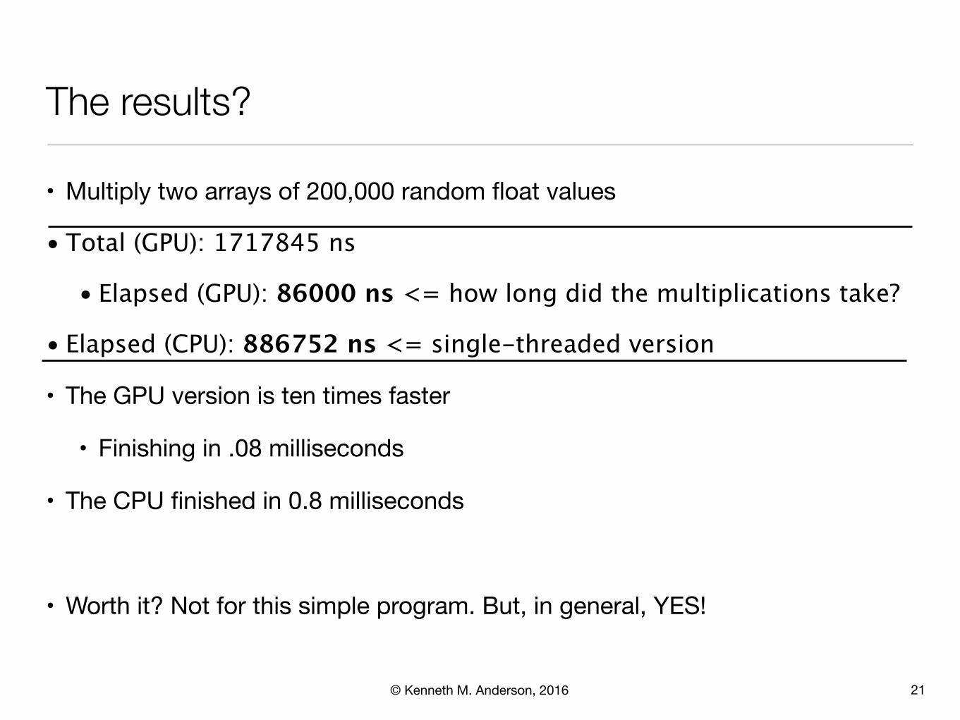
• Multiply two arrays of 200,000 random float values

• Total (GPU): 1717845 ns

• Elapsed (GPU): 86000 ns <= how long did the multiplications take?

• Elapsed (CPU): 886752 ns <= single-threaded version

• The GPU version is ten times faster

• Finishing in .08 milliseconds

• The CPU finished in 0.8 milliseconds

• Worth it? Not for this simple program. But, in general, YES!

21


Working in Multiple Dimensions

• Our first example showed how to operate on buffers that were the same length and that had a single index to organize the work

• We can work with multiple dimensions (such as multiplying matrices) by employing a common trick

• We store a multidimensional matrix into a linear array

• If we have a 2x2 matrix, we can store its values in a 4-element array

• We then use a “width” parameter and x,y coordinates to calculate where in the linear array a particular value is stored. Rather than

• a[x][y] = 10

• We write

• a[x*width+y] = 10

22


Our Second Kernel: Matrix Multiplication

23

Here’s code that implements this sequentially:

#define WIDTH_OUTPUT WIDTH_B#define HEIGHT_OUTPUT HEIGHT_A

float a[HEIGHT_A][WIDTH_A] = «initialize a»;float b[HEIGHT_B][WIDTH_B] = «initialize b»;float r[HEIGHT_OUTPUT][WIDTH_OUTPUT];

for (int j = 0; j < HEIGHT_OUTPUT; ++j) {for (int i = 0; i < WIDTH_OUTPUT; ++i) {

float sum = 0.0;for (int k = 0; k < WIDTH_A; ++k) {

sum += a[j][k] * b[k][i];}r[j][i] = sum;

}}

As you can see, as the number of elements in our array increases, the workrequired to multiply them increases dramatically, making large-matrix multi-plication a very CPU-intensive task indeed.

Parallel Matrix Multiplication

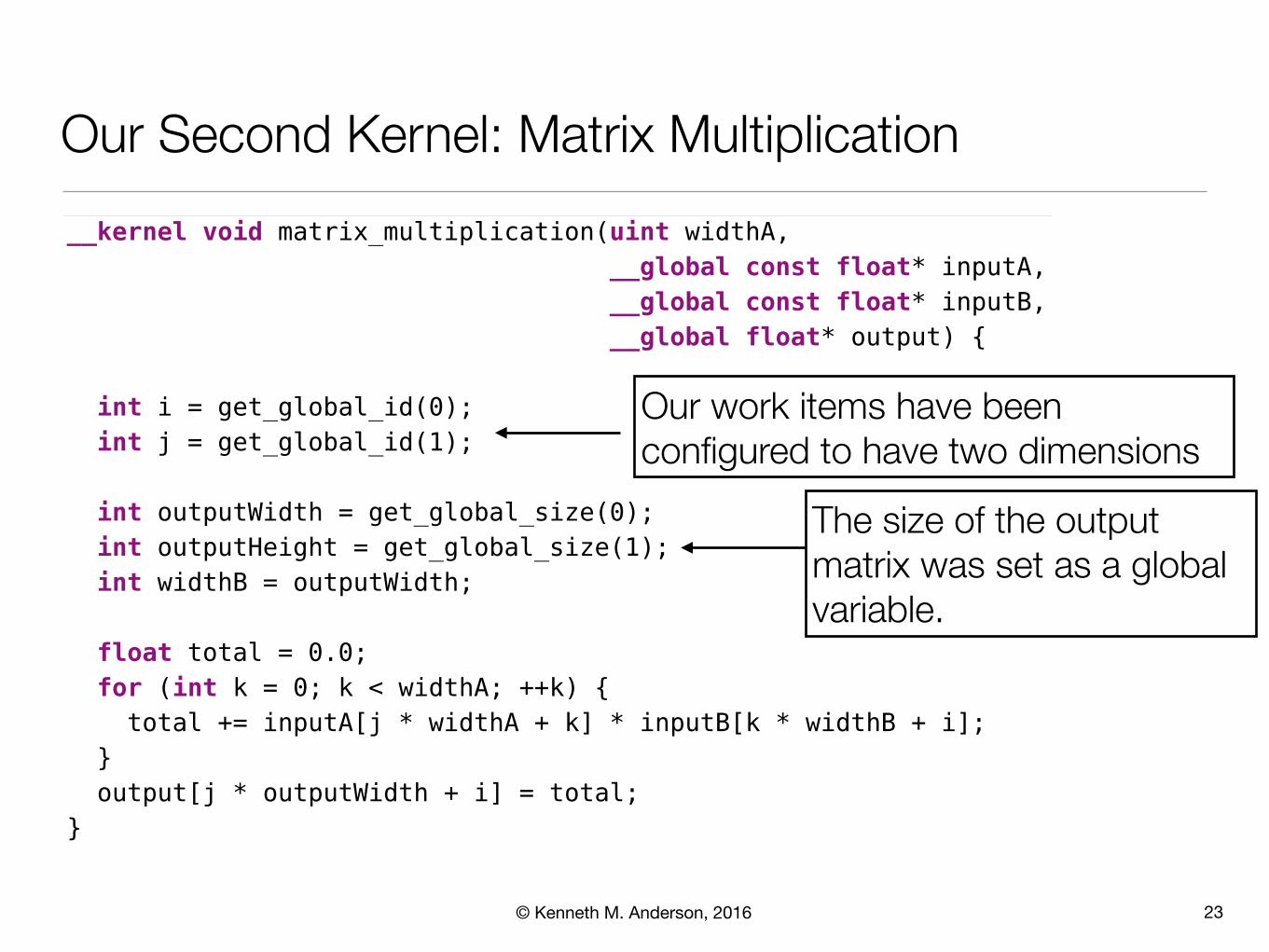
Here’s a kernel that can be used to multiply two-dimensional matrices:

DataParallelism/MatrixMultiplication/matrix_multiplication.cl__kernel void matrix_multiplication(uint widthA,Line 1

__global const float* inputA,-

__global const float* inputB,-

__global float* output) {-5

int i = get_global_id(0);-

int j = get_global_id(1);--

int outputWidth = get_global_size(0);-

int outputHeight = get_global_size(1);10

int widthB = outputWidth;--

float total = 0.0;-

for (int k = 0; k < widthA; ++k) {-

total += inputA[j * widthA + k] * inputB[k * widthB + i];15

}-

output[j * outputWidth + i] = total;-

}-

This kernel executes within a two-dimensional index space, each point ofwhich identifies a location in the output array. It retrieves this point by callingget_global_id() twice (lines 6 and 7).



Our work items have been configured to have two dimensions

The size of the output matrix was set as a global variable.


Configuring OpenCL to Work with this Kernel

24

It can find out the range of the index space by calling get_global_size(), whichthis kernel uses to find the dimensions of the output matrix (lines 9 and 10).This also gives us widthB, which is equal to outputWidth, but we have to passwidthA as a parameter.

The loop on line 14 is just the inner loop from the sequential version we sawearlier—the only difference being that because OpenCL buffers are unidimen-sional, we can’t write the following:

output[j][i] = total;

Instead, we have to use a little arithmetic to determine the correct offset:

output[j * outputWidth + i] = total;

The host program required to execute this kernel is very similar to the onewe saw yesterday, the only significant difference being the arguments passedto clEnqueueNDRangeKernel():

DataParallelism/MatrixMultiplication/matrix_multiplication.csize_t work_units[] = {WIDTH_OUTPUT, HEIGHT_OUTPUT};CHECK_STATUS(clEnqueueNDRangeKernel(queue, kernel, 2, NULL, work_units,

NULL, 0, NULL, NULL));

This creates a two-dimensional index space by setting work_dim to 2 (the thirdargument) and specifies the extent of each dimension by setting global_work_sizeto a two-element array (the fifth argument).

This kernel shows an even more dramatic performance benefit than the onewe saw yesterday. On my MacBook Pro, multiplying a 200×400 matrix by a300×200 matrix takes approximately 3 ms, compared to 66 ms on the CPU,a speedup of more than 20x.

Because this kernel is performing much more work per data element, wecontinue to see a significant speedup even if we take the overhead of copyingdata between the CPU and GPU into account. On my MacBook Pro, thosecopies take around 2 ms, for a total time of 5 ms, which still gives us a 13xspeedup.

All the code we’ve run so far simply assumes that there’s an OpenCL-compat-ible GPU available. Clearly this may not always be true, so next let’s see howwe can find out which OpenCL platforms and devices are available to a par-ticular host.


Day 2: Multiple Dimensions and Work-Groups • 203


To ensure our kernel has the information it needs, we have to change how we add work items to the queue

The “2” tells OpenCL that the work items have two dimensions

The work_units array tells OpenCL the range of the two dimensions


The results?

• The book multiplies a 200x400 matrix (of random floating point values) by a 300x200 matrix producing a 300x400 matrix as a result

• Total (GPU): 4899413 ns

• Elapsed (GPU): 3840000 ns <= 78% of the time spent multiplying

• Elapsed (CPU): 65459804 ns <= single-threaded version

• The GPU version is 17 times faster!

• Finishing in 3.84 milliseconds

• The CPU finished in 65.5 milliseconds

• Worth it? For a program that has to do a lot of these multiplications?

• YOU BET!

25


OpenCL and OpenGL: Match Made in Heaven?

• One use of OpenCL code is to work with OpenGL to perform graphics-related calculations on the GPU, freeing up the CPU to perform other operations

• OpenGL is a standard for creating 3D programs/animations

• Our book presents two OpenGL applications that make use of OpenCL to perform operations on triangles

• In the first example, we create a “mesh” of triangles and use OpenGL to display them

• we then send the vertices of the mesh to an OpenCL program that multiplies there values by 1.01 increasing the spacing of the vertices by 1% on each iteration

• This has the visual effect of zooming in on the mesh

26


Background (I)

• The mesh of triangles can be conceptualized like this

27

So in the preceding example, vertex 0 is at (0, 0, 0), vertex 1 is at (1, 0, 0),vertex 2 is at (2, 0, 0), and so on. The vertex buffer will therefore contain [0,0, 0, 1, 0, 0, 2, 0, 0, 0, 1, 0, 1, 1, 0, …].

As for the index buffer, the first triangle will use vertices 0, 1, and 3; thesecond 1, 3, and 4; the third 1, 2, and 4; and so on. The index buffer we createdefines a triangle strip in which, after specifying the first triangle with threevertices, we only need a single additional vertex to define the next triangle:

0 1 2

3 4 5

So our index buffer will contain [0, 3, 1, 4, 2, 5, …].

The code that accompanies this book includes a Mesh class that generatesinitial values for the vertex and index buffers. Our sample uses this to createa 64×64 mesh with x- and y-coordinates ranging from -1.0 to 1.0:

DataParallelism/Zoom/src/main/java/com/paulbutcher/Zoom.javaMesh mesh = new Mesh(2.0f, 2.0f, 64, 64);

The z-coordinates are all initialized to zero—we’ll modify them during anima-tion to simulate ripples.

This data is then copied to OpenGL buffers as follows:

DataParallelism/Zoom/src/main/java/com/paulbutcher/Zoom.javaint vertexBuffer = glGenBuffers();glBindBuffer(GL_ARRAY_BUFFER, vertexBuffer);glBufferData(GL_ARRAY_BUFFER, mesh.vertices, GL_DYNAMIC_DRAW);

int indexBuffer = glGenBuffers();glBindBuffer(GL_ELEMENT_ARRAY_BUFFER, indexBuffer);glBufferData(GL_ELEMENT_ARRAY_BUFFER, mesh.indices, GL_STATIC_DRAW);

Each buffer has an ID allocated by glGenBuffers(), is bound to a target withglBindBuffer(), and has its initial values set with glBufferData(). The index bufferhas the GL_STATIC_DRAW usage hint, indicating that it won’t change (is static).The vertex buffer, by contrast, has the GL_DYNAMIC_DRAW hint because it willchange between animation frames.

Before we implement the ripple code, we’ll start with something easier—asimple kernel that increases the size of the mesh over time.



There’s an index buffer that captures the existence of each index: 0, 1, 2There’s also a vertex buffer that captures the position of each index:

Index 1 => {0, 0, 0} i.e. x, y, z

So in the preceding example, vertex 0 is at (0, 0, 0), vertex 1 is at (1, 0, 0),vertex 2 is at (2, 0, 0), and so on. The vertex buffer will therefore contain [0,0, 0, 1, 0, 0, 2, 0, 0, 0, 1, 0, 1, 1, 0, …].

As for the index buffer, the first triangle will use vertices 0, 1, and 3; thesecond 1, 3, and 4; the third 1, 2, and 4; and so on. The index buffer we createdefines a triangle strip in which, after specifying the first triangle with threevertices, we only need a single additional vertex to define the next triangle:

0 1 2

3 4 5

So our index buffer will contain [0, 3, 1, 4, 2, 5, …].

The code that accompanies this book includes a Mesh class that generatesinitial values for the vertex and index buffers. Our sample uses this to createa 64×64 mesh with x- and y-coordinates ranging from -1.0 to 1.0:

DataParallelism/Zoom/src/main/java/com/paulbutcher/Zoom.javaMesh mesh = new Mesh(2.0f, 2.0f, 64, 64);

The z-coordinates are all initialized to zero—we’ll modify them during anima-tion to simulate ripples.

This data is then copied to OpenGL buffers as follows:

DataParallelism/Zoom/src/main/java/com/paulbutcher/Zoom.javaint vertexBuffer = glGenBuffers();glBindBuffer(GL_ARRAY_BUFFER, vertexBuffer);glBufferData(GL_ARRAY_BUFFER, mesh.vertices, GL_DYNAMIC_DRAW);

int indexBuffer = glGenBuffers();glBindBuffer(GL_ELEMENT_ARRAY_BUFFER, indexBuffer);glBufferData(GL_ELEMENT_ARRAY_BUFFER, mesh.indices, GL_STATIC_DRAW);

Each buffer has an ID allocated by glGenBuffers(), is bound to a target withglBindBuffer(), and has its initial values set with glBufferData(). The index bufferhas the GL_STATIC_DRAW usage hint, indicating that it won’t change (is static).The vertex buffer, by contrast, has the GL_DYNAMIC_DRAW hint because it willchange between animation frames.

Before we implement the ripple code, we’ll start with something easier—asimple kernel that increases the size of the mesh over time.



When we create the vertex buffer, we tell OpenGL that it will change


Background (II)

• Our kernel for zooming is simple

• get each value, (x, y, z), and increase its size by 1%

28

Accessing an OpenGL Buffer from an OpenCL KernelHere’s the kernel that implements our zoom animation:

DataParallelism/Zoom/src/main/resources/zoom.cl__kernel void zoom(__global float* vertices) {

unsigned int id = get_global_id(0);vertices[id] *= 1.01;

}

It takes the vertex buffer as an argument and multiplies every entry in thatbuffer by 1.01, increasing the size of the mesh by 1% every time it’s called.

Before we can pass the vertex buffer to our kernel, we first need to create anOpenCL buffer that references it:

DataParallelism/Zoom/src/main/java/com/paulbutcher/Zoom.javaCLMem vertexBufferCL =

clCreateFromGLBuffer(context, CL_MEM_READ_WRITE, vertexBuffer, null);

This buffer object can then be used in our main rendering loop as follows:

DataParallelism/Zoom/src/main/java/com/paulbutcher/Zoom.javawhile (!Display.isCloseRequested()) {

glClear(GL_COLOR_BUFFER_BIT | GL_DEPTH_BUFFER_BIT);glLoadIdentity();glTranslatef(0.0f, 0.0f, planeDistance);glDrawElements(GL_TRIANGLE_STRIP, mesh.indexCount, GL_UNSIGNED_SHORT, 0);

Display.update();

Util.checkCLError(clEnqueueAcquireGLObjects(queue, vertexBufferCL, null, null));➤kernel.setArg(0, vertexBufferCL);➤clEnqueueNDRangeKernel(queue, kernel, 1, null, workSize, null, null, null);➤Util.checkCLError(clEnqueueReleaseGLObjects(queue, vertexBufferCL, null, null));➤clFinish(queue);➤

}

Before an OpenCL kernel can use an OpenGL buffer, we need to acquire itwith clEnqueueAcquireGLObjects(). We can then set it as an argument to our kerneland call clEnqueueNDRangeKernel() as normal. Finally, we release the buffer withclEnqueueReleaseGLObjects() and wait for the commands we’ve dispatched to finishwith clFinish().

Run this code, and you should see the mesh start out small and quickly growto the point that a single triangle fills the screen.

Now that we’ve got a simple animation working that integrates OpenGL withOpenCL, we’ll look at the more sophisticated kernel that implements ourwater ripples.


Day 3: OpenCL and OpenGL—Keeping It on the GPU • 215



Background (III)

• The key to making this work is to then associate an OpenGL buffer with an OpenCL buffer

• In a loop do the following

• draw the OpenGL buffer

• associate the OpenGL buffer with an OpenCL buffer

• allow OpenCL to apply the kernel to the OpenCL buffer (which changes the OpenGL buffer automatically)

• call “finish” to ensure that all OpenCL operations have completed

• OpenGL will then draw the new mesh, the next time through the loop

29


Background (IV): In Code

30

Accessing an OpenGL Buffer from an OpenCL KernelHere’s the kernel that implements our zoom animation:

DataParallelism/Zoom/src/main/resources/zoom.cl__kernel void zoom(__global float* vertices) {

unsigned int id = get_global_id(0);vertices[id] *= 1.01;

}

It takes the vertex buffer as an argument and multiplies every entry in thatbuffer by 1.01, increasing the size of the mesh by 1% every time it’s called.

Before we can pass the vertex buffer to our kernel, we first need to create anOpenCL buffer that references it:

DataParallelism/Zoom/src/main/java/com/paulbutcher/Zoom.javaCLMem vertexBufferCL =clCreateFromGLBuffer(context, CL_MEM_READ_WRITE, vertexBuffer, null);

This buffer object can then be used in our main rendering loop as follows:

DataParallelism/Zoom/src/main/java/com/paulbutcher/Zoom.javawhile (!Display.isCloseRequested()) {glClear(GL_COLOR_BUFFER_BIT | GL_DEPTH_BUFFER_BIT);glLoadIdentity();glTranslatef(0.0f, 0.0f, planeDistance);glDrawElements(GL_TRIANGLE_STRIP, mesh.indexCount, GL_UNSIGNED_SHORT, 0);

Display.update();

Util.checkCLError(clEnqueueAcquireGLObjects(queue, vertexBufferCL, null, null));➤kernel.setArg(0, vertexBufferCL);➤clEnqueueNDRangeKernel(queue, kernel, 1, null, workSize, null, null, null);➤Util.checkCLError(clEnqueueReleaseGLObjects(queue, vertexBufferCL, null, null));➤clFinish(queue);➤

}

Before an OpenCL kernel can use an OpenGL buffer, we need to acquire itwith clEnqueueAcquireGLObjects(). We can then set it as an argument to our kerneland call clEnqueueNDRangeKernel() as normal. Finally, we release the buffer withclEnqueueReleaseGLObjects() and wait for the commands we’ve dispatched to finishwith clFinish().

Run this code, and you should see the mesh start out small and quickly growto the point that a single triangle fills the screen.

Now that we’ve got a simple animation working that integrates OpenGL withOpenCL, we’ll look at the more sophisticated kernel that implements ourwater ripples.




DEMO


Ripple (I)

• In the previous example, the z values were initialized to zero

• And, 0 * 1.01 == 0

• As a result, the “zoom” of the previous example was achieved by just spacing out the triangles' x and y values until they were offscreen

• The second example is more interesting, the kernel targets the z value of a triangle’s vertices

• As a result, it will morph the mesh into “3D shapes”

• And, just to be fancy, the program supports up to 16 ripples at a time!

31


Ripple (II)

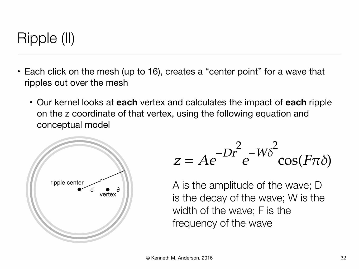
• Each click on the mesh (up to 16), creates a “center point” for a wave that ripples out over the mesh

• Our kernel looks at each vertex and calculates the impact of each ripple on the z coordinate of that vertex, using the following equation and conceptual model

32

Within the loop, we examine each ripple center with a nonzero start time inturn. For each, we start by determining the distance d between the pointwe’re calculating and the ripple center (line 21). Next, we calculate the radiusr of the expanding ripple ring (line 23) and δ , the distance between our pointand this ripple ring (line 24):

r

dripple center

vertex

Finally, we can combine δ and r to get z :

Here, A , D , W , and F are constants representing the amplitude of the wavepacket, the rate at which it decays as it expands, the width of the wavepacket, and the frequency, respectively.

The final piece of the puzzle is to extend our host application to create ourripple centers:

DataParallelism/Ripple/src/main/java/com/paulbutcher/Ripple.javaint numCenters = 16;int currentCenter = 0;FloatBuffer centers = BufferUtils.createFloatBuffer(numCenters * 2);centers.put(new float[numCenters * 2]);centers.flip();LongBuffer times = BufferUtils.createLongBuffer(numCenters);times.put(new long[numCenters]);times.flip();

CLMem centersBuffer =clCreateBuffer(context, CL_MEM_READ_ONLY | CL_MEM_COPY_HOST_PTR,centers, null);

CLMem timesBuffer =clCreateBuffer(context, CL_MEM_READ_ONLY | CL_MEM_COPY_HOST_PTR, times, null);

And start a new ripple whenever the mouse is clicked:




Within the loop, we examine each ripple center with a nonzero start time inturn. For each, we start by determining the distance d between the pointwe’re calculating and the ripple center (line 21). Next, we calculate the radiusr of the expanding ripple ring (line 23) and δ , the distance between our pointand this ripple ring (line 24):

r

dripple center

vertex

Finally, we can combine δ and r to get z :

z = Ae−Dr2e−Wδ

2cos(Fπδ)

Here, A , D , W , and F are constants representing the amplitude of the wavepacket, the rate at which it decays as it expands, the width of the wavepacket, and the frequency, respectively.

The final piece of the puzzle is to extend our host application to create ourripple centers:

DataParallelism/Ripple/src/main/java/com/paulbutcher/Ripple.javaint numCenters = 16;int currentCenter = 0;FloatBuffer centers = BufferUtils.createFloatBuffer(numCenters * 2);centers.put(new float[numCenters * 2]);centers.flip();LongBuffer times = BufferUtils.createLongBuffer(numCenters);times.put(new long[numCenters]);times.flip();

CLMem centersBuffer =clCreateBuffer(context, CL_MEM_READ_ONLY | CL_MEM_COPY_HOST_PTR,centers, null);

CLMem timesBuffer =clCreateBuffer(context, CL_MEM_READ_ONLY | CL_MEM_COPY_HOST_PTR, times, null);

And start a new ripple whenever the mouse is clicked:




A is the amplitude of the wave; D is the decay of the wave; W is the width of the wave; F is the frequency of the wave


Ripple (III): The Kernel

33

Simulating RipplesWe’re going to simulate expanding rings of ripples. Each expanding ring isdefined by a 2D point on the mesh (the center of the expanding ring) togetherwith a time (the time at which the ring started expanding). As well as takinga pointer to the OpenGL vertex buffer, our kernel takes an array of ripplecenters together with a corresponding array of times (where time is measuredin milliseconds):

DataParallelism/Ripple/src/main/resources/ripple.cl#define AMPLITUDE 0.1Line 1

#define FREQUENCY 10.0-

#define SPEED 0.5-

#define WAVE_PACKET 50.0-

#define DECAY_RATE 2.05

__kernel void ripple(__global float* vertices,-

__global float* centers,-

__global long* times,-

int num_centers,-

long now) {10

unsigned int id = get_global_id(0);-

unsigned int offset = id * 3;-

float x = vertices[offset];-

float y = vertices[offset + 1];-

float z = 0.0;15-

for (int i = 0; i < num_centers; ++i) {-

if (times[i] != 0) {-

float dx = x - centers[i * 2];-

float dy = y - centers[i * 2 + 1];20

float d = sqrt(dx * dx + dy * dy);-

float elapsed = (now - times[i]) / 1000.0;-

float r = elapsed * SPEED;-

float delta = r - d;-

z += AMPLITUDE *25

exp(-DECAY_RATE * r * r) *-

exp(-WAVE_PACKET * delta * delta) *-

cos(FREQUENCY * M_PI_F * delta);-

}-

}30

vertices[offset + 2] = z;-

}-

We start by determining the x- and y-coordinates of the vertex that’s beingprocessed by the current work-item (lines 13 and 14). In the loop (lines 17–30)we calculate a new z-coordinate that we write back to the vertex buffer online 31.



Three arrays are passed along with two parameters to each one-dimensional work item

Our id retrieves the vertex that we’re working on. The centers array contains the center point of each ripple. The times array contains the time each ripple was created. The now variable contains the current time.

With that information, we can use the equation on the previous slide, to update the z value for each ripple

OpenCL ensures that ALL vertices are updated IN PARALLEL. That’s the true power of this approach. DEMO


Summary

• We scratched the surface of data parallelism and GPU programming with OpenCL

• We looked at a range of examples of OpenCL kernels

• an abstract way of defining a “work item”

• This specification is compiled into code that performs the specified operations on as many data points as possible in parallel

• We saw the power of this technique by showing how OpenCL can support the transformation of OpenGL objects, the GPU performs most of the calculations, freeing up the CPU to handle other tasks

• This approach stands in contrast to the other concurrency alternatives

• our programs were all single threaded; instead we used the GPU to perform calculations in parallel when it was needed

34

data parallelism - computer science · • data parallelism • using opencl to create ... allows...

Documents