Data Mining with Neural Networks

• Standard data mining terminology• Preprocessing data• Running neural networks via Analyze/StripMiner• Cherkassky’s nonlinear regression problem• Magnetocardiogram data• CBA (chemical and biological agents) Data• Drug design with neural networks• The paradox of learning• Principal Component Analysis (PCA)• The Kernel Transformation and SVMs (Support Vector Machines)• Structural and empirical risk minimization (Vapnik’s theory of statistical learning)

• Basic Terminology - MetaNeural Format - Descriptors, features, response (or activity) and ID - Classification versus regression - Modeling/Feature detection - Training/Validation/Calibration - Vertical and horizontal view of data

• Outliers, rare events and minority classes• Data Preparation

- Data cleansing - Scaling

• Leave-one-out and leave-several-out validation• Confusion matrix and ROC curves

Standard Data Mining Terminology

Installing Basic Version of Analyze

• Put analyze and gnuplot and wgnuplt.hlp and wgnuplot.mnu in working folder• gnuplot scripts for plotting are: - analyze resultss.ttt –3305 for scatterplot - analyze resultss.ttt –3313 for errorplot - analyze resultss.ttt –3362 for baniary classification• More fancy graphics are in the *.jar files (needs java runtime environment)• For basic help you can try: - analyze > readme.txt - analyze help –998 - analyze help –997 - analyze help –008• For beginners (unless the Java runtime environment is installed), I recommend displaying results via gnuplot operators –3305, -3313 and –3362• To familiarize with Analyze, study the script files from this handout• Don’t forget to scale data

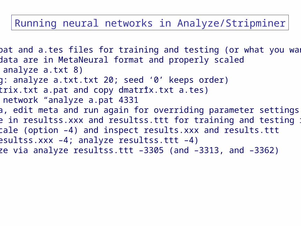
Running neural networks in Analyze/Stripminer

• Prepare a.pat and a.tes files for training and testing (or what you want to name it)• Make sure data are in MetaNeural format and properly scaled (scaling: analyze a.txt 8) (splitting: analyze a.txt.txt 20; seed ‘0’ keeps order) (copy cmatrix.txt a.pat and copy dmatrix.txt a.tes)• Run neural network “analyze a.pat 4331”• copy a meta, edit meta and run again for overriding parameter settings• Results are in resultss.xxx and resultss.ttt for training and testing respectively• Either descale (option –4) and inspect results.xxx and results.ttt (analyze resultss.xxx –4; analyze resultss.ttt –4)• Or visualize via analyze resultss.ttt –3305 (and –3313, and –3362)

A Vertical and a Horizontal View of the Data Matrix

• Vertical view: feature space

Miaaaaa

NjaA

ijNMijjTj

TjNM

,1for ......

,1for

1

�

• Horizontal view: data space

Nx

x

x

A

�

...2

1

iiiMiii IDyaaax ...21

Preprocessing: Basic scaling for neural networks

• Mahalanobis scale descriptors

• [0-1] scale response

• Use operator 8 in Analyze code: e.g., typing “analyze a.pat 8” will give scaled results in a.pat.txt• Note: another handy operator is the splitting operator (20) e.g., typing < analyze a.pat.txt 20> will split file in cmatrix.txt and dmatrix.txt usimg 0 as random number seed put the first #data in cmatrix.txt using a different seed scrambles up data

x

xxx

minmax

min

yy

yyy

0.7

0.8

0.9

1

1.1

1.2

1.3

1.4

0 10 20 30 40 50 60 70 80 90 100

Targ

et and P

redic

ted V

alu

es

Sorted Sequence Number

Errorplot for Test Data

Thu Mar 13 19:28:39 2003

targetpredicted

Cherkassky’s Nonlinear Benchmark Data

• Generate 500 data (400 training; 100 testing)

• Impossible data for linear models

25.025.0

sinsin2exp 3241

x

xxxxy

0.7

0.8

0.9

1

1.1

1.2

1.3

1.4

0 10 20 30 40 50 60 70 80 90 100

Targ

et and P

redic

ted V

alu

es

Sorted Sequence Number

Errorplot for Test Data

Thu Mar 13 18:14:14 2003

targetpredicted

K-PLS

PLS

REM cherkasmREM GENERATE DATA (2 500 2)

analyze a.pat 3301REM SCALE DATA

analyze cherkas.pat 8REM SPLIT DATA IN TRAINING AND TEST SET (400 2)

analyze cherkas.pat.txt 20copy cmatrix.txt a.patcopy dmatrix.txt a.tes

REM RUN METANEURAL VIA ANALYZEanalyze a.pat 4331

DESCALE RESULTSanalyze resultss.ttt -4

REM VISUALIZE RESULTS FOR TEST SETanalyze resultss.ttt -3305pauseanalyze resultss.ttt -3313pausegnuplot error1.pltpause

REM VISUALIZE RESULTS FOR TRAINING SETanalyze resultss.xxx -3305pauseanalyze resultss.xxx -3313pause

Note: eta = 0.01; train to 0.02 error

Iris Data

REM IRISM.BAT (3 classes)REM GENERATE DATA (5)

analyze iris 3301REM STRIP HEADER

analyze iris.txt 100REM SCALE DATA

analyze iris.txt.txt 8copy iris.txt.txt.txt a.txt

REM SPLIT DATA (100 2)analyze a.txt 20copy cmatrix.txt a.patcopy dmatrix.txt a.tes

REM METANEURALREM do copy a meta afterwards to customize

analyze a.pat 4331pause

REM SCATTERPLOT FOR TEST DATAanalyze resultss.ttt -3305pause

REM ERRORPLOT FOR TEST DATAanalyze resultss.ttt -3313pause

REM SCATTERPLOT FOR TRAINING DATAanalyze resultss.xxx -3305pause

REM ERRORPLOT FOR TRAINING DATAanalyze resultss.xxx -3313pause

1

1.5

2

2.5

3

0 5 10 15 20 25 30 35 40 45 50Target

an

d P

redic

ted V

alu

es

Sorted Sequence Number

Errorplot for Test Data

Sun Mar 16 16:11:07 2003

predictedtarget

For homework:- copy a meta- Edit meta for different experiments- summarize and report on experiments

1,1,

1

1

1

1

1

1

1

11

11

11

ˆ mmtesttest

nTmnnm

Tmnm

nTmnnm

Tmnmnm

Tmnnm

Tmn

nTmnmnm

Tmn

nTmnmnm

Tmn

nmnm

wXy

yXXXw

yXXXwXXXX

yXwXX

yXwXX

ywX

Pseudo inverse

Classical Regression Analysis

NAME PIE PIF DGR SAC MR Lam Vol DDGTS IDAla 0.23 0.31 -0.55 254.2 2.126 -0.02 82.2 8.5 0Asn -0.48 -0.6 0.51 303.6 2.994 -1.24 112.3 8.2 1Asp -0.61 -0.77 1.2 287.9 2.994 -1.08 103.7 8.5 2Cys 0.45 1.54 -1.4 282.9 2.933 -0.11 9.1 11 3Gln -0.11 -0.22 0.29 335 3.458 -1.19 127.5 6.3 4Glu -0.51 -0.64 0.76 311.6 3.243 -1.43 120.5 8.8 5Gly 0 0 0 224.9 1.662 0.03 65 7.1 6His 0.15 0.13 -0.25 337.2 3.856 -1.06 140.6 10.1 7Ile 1.2 1.8 -2.1 322.6 3.35 0.04 131.7 16.8 8

Leu 1.28 1.7 -2 324 3.518 0.12 131.5 15 9Lys -0.77 -0.99 0.78 336.6 2.933 -2.26 144.3 7.9 10Met 0.9 1.23 -1.6 336.3 3.86 -0.33 132.3 13.3 11Phe 1.56 1.79 -2.6 366.1 4.638 -0.05 155.8 11.2 12Pro 0.38 0.49 -1.5 288.5 2.876 -0.31 106.7 8.2 13Ser 0 -0.04 0.09 266.7 2.279 -0.4 88.5 7.4 14Thr 0.17 0.26 -0.58 283.9 2.743 -0.53 105.3 8.8 15Trp 1.85 2.25 -2.7 401.8 5.755 -0.31 185.9 9.9 16Tyr 0.89 0.96 -1.7 377.8 4.791 -0.84 162.7 8.8 17Val 0.71 1.22 -1.6 295.1 3.054 -0.13 115.6 12 18

A

c

LS-SVM

11

1

11

nnnn

nnnn

yIKw

ywK

• Adding the ridge makes the matrix positive definite• The ridge also performs regularization!!!!• The problem is now equivalent to minimizing the following:

2

2

1

ˆ wyyN

iii

Heuristic formula for lambda

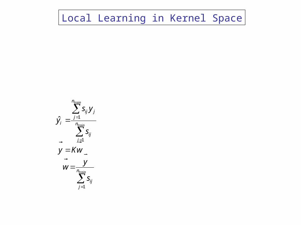
Local Learning in Kernel Space

train

train

train

n

jij

n

jij

n

jjij

i

s

yw

wKy

s

ys

y

1

1

1ˆ

x1

xM

xi

Σ

Σ

Σ

Σ

Σ

Σ

Σ

Σ

1y

My

iy iy

Weights correspond tothe dependent variable

for the entire training data

1

1

trainn

iijs

This layer gives a similarity scorewith each datapoint

Kind of a nearestneighbor weighted

prediction score

22ji xx

ij es

Make up kernels

Local Learning in Kernel Space

train

train

train

n

jij

n

jij

n

jjij

i

s

yw

wKy

s

ys

y

1

1

1ˆ

Kernel, KNN

w1

wN

wi

NxN

Ny

predictionWeight vector

(Data Set)NxM

• K-PLS is like a linear method in “nonlinear kernel” space

• Kernel space is the “latent space” of support vector machines (SVMs)

• How to make LS-SVM work? - Select kernel transformation (e.g., usually a Gaussian kernel)

- Select regularization parameter

What Does LS-SVM Do?

NNNN ywK ˆ

What is in a Kernel?

• A kernel can be considered as a (nonlinear) data transformation - Many different choices for the kernel are possible - Most popular is the Radial Basis Function or Gaussian kernel

• The Gaussian kernel is a symmetric matrix - Entries reflect nonlinear similarities amongst data descriptions

- As defined by:

22

2lj xx

ij ek

NNNN

iNijii

N

N

NN

kkk

kkkk

kkk

kkk

K

...

...

...

21

21

22221

11211

�

x1

x2

x3

t1

t2

y

PharmaPlot

Wed Mar 19 15:23:32 2003

'negative''positive'

-0.08-0.06-0.04-0.02 0 0.02 0.04First PLS Component -0.06-0.04

-0.02 0

0.02 0.04

0.06 0.08

Second PLS Component

-0.08-0.06-0.04-0.02

0 0.02 0.04 0.06 0.08 0.1

Third PLS Component

Data Visualization with Cardiomag Program

cardiomag patients.txt 402

patients.txt

pat1.txt.txt

pat2.txt.txt

…

vis.txt

vis.txt.txt

pat_ID.jpg

pat_view.jar

data visualization mode(requires Java run time environment)

Raw data

Wavelet transformed data

wave_val.cat

0 20 40-5

0

5

0 20 40-2

0

2

0 20 40-2

0

2

0 20 40-2

0

2

0 20 40-2

0

2

0 20 40-2

0

2

0 20 40-2

0

2

0 20 40-2

0

2

0 20 40-2

0

2

0 20 40-2

0

2

0 20 40-2

0

2

0 20 40-2

0

2

0 20 40-5

0

5

0 20 40-2

0

2

0 20 40-2

0

2

0 20 40-5

0

5

0 20 40-2

0

2

0 20 40-2

0

2

0 20 40-5

0

5

0 20 40-2

0

2

0 20 40-2

0

2

0 20 40-2

0

2

0 20 40-2

0

2

0 20 40-2

0

2

0 20 40-5

0

5

0 20 40-5

0

5

0 20 40-2

0

2

0 20 40-2

0

2

0 20 40-2

0

2

0 20 40-2

0

2

0 20 40-2

0

2

0 20 40-2

0

2

0 20 40-2

0

2

0 20 40-2

0

2

0 20 40-2

0

2

0 20 40-2

0

2

DATA FOR PATIENT 97

Worth its Weight in Gold?

Data Mining Applications In DDASSL

• QSAR drug design• Microarrays• Breast Cancer Diagnosis(TransScan)

Molecule #BR #C #CL #F #H #I #N #O #P #S #SI BALA IDC IDCBAR IDW IDWBAR K0 K1 K2K3 KA1 KA2 KA3 NXC3 NXC4 NXCH10 NXCH3 NXCH4 NXCH5 NXCH6 NXCH7 NXCH8 NXCH9NXP10 NXP2 NXP3 NXP4 NXP5 NXP6 NXP7 NXP8 NXP9 NXPC4 SI TOPOL90 TOPOL91TOPOL92 TOPOL93 TOPOL94 TOPOL95 TOPOL96 TOPOL97 TOPOL98 TOPOL99 WW X0 X1 X2XC3 XC4 XCH10 XCH3 XCH4 XCH5 XCH6 XCH7 XCH8 XCH9 XP10 XP3 XP4 XP5 XP6 XP7XP8 XP9 XPC4 XV0 XV1 XV2 XVC3 XVC4 XVCH10 XVCH3 XVCH4 XVCH5 XVCH6 XVCH7XVCH8 XVCH9 XVP10 XVP3 XVP4 XVP5 XVP6 XVP7 XVP8 XVP9 XVPC4 S001 S002 S003S004 S005 S006 S007 S008 S009 S010 S011 S012 S013 S014 S015 S016 S017 S018 S019S020 S021 S022 S023 S024 S025 S026 S027 S028 S029 S030 S031 S032 S033 S034 S035S036 S037 S038 S039 S040 S041 S042 S043 S044 S045 S046 S047 S048 S049 S050 S051S052 S053 S054 S055 S056 S057 S058 S059 S060 S061 S062 S063 S064 S065 S066 S067S068 S069 S070 S071 S072 S073 S074 S075 S076 S077 S078 S079 S080 S081 S082 S083S084 S085 S086 S087 S088 S089 S090 S091 S092 S093 S094 S095 S096 S097 S098 S099S100 S101 S102 S103 S104 S105 S106 S107 S108 S109 S110 S111 S112 S113 S114 S115S116 S117 S118 S119 S120 S121 S122 S123 S124 S125 S126 S127 S128 S129 S130 S131S132 S133 S134 S135 S136 S137 S138 S139 S140 S141 S142 S143 S144 S145 S146 S147S148 S149 S150 S151 S152 S153 S154 S155 S156 S157 S158 S159 S160 S161 S162 S163S164 S165 S166 S167 S168 S169 S170 S171 S172 S173 S174 S175 S176 S177 S178 S179S180 S181 S182 S183 S184 S185 S186 S187 S188 S189 S190 S191 S192 S193 S194 S195S196 S197 S198 S199 S200 S201 S202 S203 S204 S205 S206 S207 S208 AbsBNP1 AbsBNP10AbsBNP2 AbsBNP3 AbsBNP4 AbsBNP5 AbsBNP6 AbsBNP7 AbsBNP8 AbsBNP9 AbsBNPMaxAbsBNPMin AbsDGN1 AbsDGN10 AbsDGN2 AbsDGN3 AbsDGN4 AbsDGN5 AbsDGN6 AbsDGN7AbsDGN8 AbsDGN9 AbsDGNMax AbsDGNMin AbsDKN1 AbsDKN10 AbsDKN2 AbsDKN3 AbsDKN4AbsDKN5 AbsDKN6 AbsDKN7 AbsDKN8 AbsDKN9 AbsDKNMax AbsDKNMin AbsDRN1 AbsDRN10AbsDRN2 AbsDRN3 AbsDRN4 AbsDRN5 AbsDRN6 AbsDRN7 AbsDRN8 AbsDRN9 AbsDRNMaxAbsDRNMin AbsEP1 AbsEP10 AbsEP2 AbsEP3 AbsEP4 AbsEP5 AbsEP6 AbsEP7 AbsEP8 AbsEP9AbsEPMax AbsEPMin AbsFuk1 AbsFuk10 AbsFuk2 AbsFuk3 AbsFuk4 AbsFuk5 AbsFuk6 AbsFuk7AbsFuk8 AbsFuk9 AbsFukMax AbsFukMin AbsG1 AbsG10 AbsG2 AbsG3 AbsG4 AbsG5 AbsG6AbsG7 AbsG8 AbsG9 AbsGMax AbsGMin AbsK1 AbsK10 AbsK2 AbsK3 AbsK4 AbsK5 AbsK6AbsK7 AbsK8 AbsK9 AbsKMax AbsKMin AbsL1 AbsL10 AbsL2 AbsL3 AbsL4 AbsL5 AbsL6 AbsL7AbsL8 AbsL9 AbsLMax AbsLMin BNP BNP1 BNP10 BNP2 BNP3 BNP4 BNP5 BNP6 BNP7 BNP8BNP9 BNPAvg BNPMax BNPMin Del(G)NA1 Del(G)NA10 Del(G)NA2 Del(G)NA3 Del(G)NA4 Del(G)NA5Del(G)NA6 Del(G)NA7 Del(G)NA8 Del(G)NA9 Del(G)NIA Del(G)NMax Del(G)NMin Del(K)IA Del(K)MaxDel(K)Min Del(K)NA1 Del(K)NA10 Del(K)NA2 Del(K)NA3 Del(K)NA4 Del(K)NA5 Del(K)NA6 Del(K)NA7Del(K)NA8 Del(K)NA9 Del(Rho)NA1 Del(Rho)NA10 Del(Rho)NA2 Del(Rho)NA3 Del(Rho)NA4Del(Rho)NA5 Del(Rho)NA6 Del(Rho)NA7 Del(Rho)NA8 Del(Rho)NA9 Del(Rho)NIA Del(Rho)NMaxDel(Rho)NMin EP1 EP10 EP2 EP3 EP4 EP5 EP6 EP7 EP8 EP9 Fuk Fuk1 Fuk10 Fuk2 Fuk3Fuk4 Fuk5 Fuk6 Fuk7 Fuk8 Fuk9 FukAvg FukMax FukMin Lapl Lapl1 Lapl10 Lapl2 Lapl3Lapl4 Lapl5 Lapl6 Lapl7 Lapl8 Lapl9 LaplAvg LaplMax LaplMin PIP1 PIP10 PIP11 PIP12 PIP13PIP14 PIP15 PIP16 PIP17 PIP18 PIP19 PIP2 PIP20 PIP3 PIP4 PIP5 PIP6 PIP7 PIP8 PIP9PIPAvg PIPMax PIPMin piV SIDel(G)N SIDel(K)N SIDel(Rho)N SIEP SIEPA1 SIEPA10 SIEPA2SIEPA3 SIEPA4 SIEPA5 SIEPA6 SIEPA7 SIEPA8 SIEPA9 SIEPIA SIEPMax SIEPMin SIG SIGA1SIGA10 SIGA2 SIGA3 SIGA4 SIGA5 SIGA6 SIGA7 SIGA8 SIGA9 SIGIA sigmanew sigmaNVsigmaPV SIGMax SIGMin SIK SIKA1 SIKA10 SIKA2 SIKA3 SIKA4 SIKA5 SIKA6 SIKA7 SIKA8SIKA9 SIKIA SIKMax SIKMin sumsigma SurfArea Volume CAQSOL CHEM_POT CLOGP CMRCSAREA_A CSAREA_B CSAREA_C DELTAHF DIPOLE ETOT EVDW HARDNESS HBAB HBDA HOMOLENGTH_A LENGTH_B LENGTH_C LUMO MASS MUA MUB MUC NHBA NHBD NUMHB PISUBIQMINUS QPLUS RA RB RC SAAB SAAC SABC SAREA SASAREA SASVOL SHAPE VLOOP1VLOOP2 VLOOP3 VLOOP4 VLOOP5 VOLUME

CO1CO2CO3CO4CO5CO6CO7CO8CO9C10

. . .

C66T1C11T2C1T2C11T2C13T2C16T2C1T2C9

LCCKA Log(10) of inhibition concentration for "A" receptor site on Cholecystokinin

1 ) Surface properties are encoded on 0.002 e/au3 surface Breneman, C.M. and Rhem, M. [1997] J. Comp. Chem., Vol. 18 (2), p. 182-197

2 ) Histograms or wavelet encoded of surface properties give TAE property descriptors

Electron Density-Derived TAE-Wavelet Descriptors

PIP (Local Ionization Potential)

Histograms

Wavelet Coefficients

Validation Model: 100x leave 10% out validations

StripMiner with Feature Selection and Bootstrapping/Bagging

RAW DATA

Pre-processing: - scaling - ANN policy Sensitivity Analysis

Learning Algorithm

Neural NetworkSVMPLS

RANDOM GAUGEVARIABLE

REDUCEDFEATURE SET

bootstrapping

Bagging Prediction

Neural NetworkSVMPLS

PREDICTIVE MODEL

PLS, K-PLS, SVM, ANN

0.05

0.1

0.15

0.2

0.25

0.3

0.35

0.4

0.45

0 100 200 300 400 500 600

1 -

Q2

# Features

1 - Q2 versus # Features on Validation Set

Thu Mar 13 15:59:57 2003

'evolve.txt' using 1:2

Data StripMining Approach for Feature Selection

Kernel PLS (K-PLS)

x1

x2

x3

t1

t2

y

• Introduced by Rosipal and Trejo (J. Machine Learning, December 2001)• K-PLS gives almost identical (but more stable) results to SVMs for QSAR data - K-PLS is more transparent. - K-PLS allows to visualize in SVM Space - Computationally efficient and few heuristics - There is no patent on K-PLS• Consider K-PLS as a “better” nonlinear PLS

• Binding affinities to human serum albumin (HSA): log K’hsa• Gonzalo Colmenarejo, GalaxoSmithKline J. Med. Chem. 2001, 44, 4370-4378

• 95 molecules, 250-1500+ descriptors• 84 training, 10 testing (1 left out)• 551 Wavelet + PEST + MOE descriptors• Widely different compounds• Acknowledgements: Sean Eakins (Concurrent) N. Sukumar (Rensselaer)

GATCAATGAGGTGGACACCAGAGGCGGGGACTTGTAAATAACACTGGGCTGTAGGAGTGA

TGGGGTTCACCTCTAATTCTAAGATGGCTAGATAATGCATCTTTCAGGGTTGTGCTTCTA

TCTAGAAGGTAGAGCTGTGGTCGTTCAATAAAAGTCCTCAAGAGGTTGGTTAATACGCAT

GTTTAATAGTACAGTATGGTGACTATAGTCAACAATAATTTATTGTACATTTTTAAATAG

CTAGAAGAAAAGCATTGGGAAGTTTCCAACATGAAGAAAAGATAAATGGTCAAGGGAATG

GATATCCTAATTACCCTGATTTGATCATTATGCATTATATACATGAATCAAAATATCACA

CATACCTTCAAACTATGTACAAATATTATATACCAATAAAAAATCATCATCATCATCTCC

ATCATCACCACCCTCCTCCTCATCACCACCAGCATCACCACCATCATCACCACCACCATC

ATCACCACCACCACTGCCATCATCATCACCACCACTGTGCCATCATCATCACCACCACTG

TCATTATCACCACCACCATCATCACCAACACCACTGCCATCGTCATCACCACCACTGTCA

TTATCACCACCACCATCACCAACATCACCACCACCATTATCACCACCATCAACACCACCA

CCCCCATCATCATCATCACTACTACCATCATTACCAGCACCACCACCACTATCACCACCA

CCACCACAATCACCATCACCACTATCATCAACATCATCACTACCACCATCACCAACACCA

CCATCATTATCACCACCACCACCATCACCAACATCACCACCATCATCATCACCACCATCA

CCAAGACCATCATCATCACCATCACCACCAACATCACCACCATCACCAACACCACCATCA

CCACCACCACCACCATCATCACCACCACCACCATCATCATCACCACCACCGCCATCATCA

TCGCCACCACCATGACCACCACCATCACAACCATCACCACCATCACAACCACCATCATCA

CTATCGCTATCACCACCATCACCATTACCACCACCATTACTACAACCATGACCATCACCA

CCATCACCACCACCATCACAACGATCACCATCACAGCCACCATCATCACCACCACCACCA

CCACCATCACCATCAAACCATCGGCATTATTATTTTTTTAGAATTTTGTTGGGATTCAGT

ATCTGCCAAGATACCCATTCTTAAAACATGAAAAAGCAGCTGACCCTCCTGTGGCCCCCT

TTTTGGGCAGTCATTGCAGGACCTCATCCCCAAGCAGCAGCTCTGGTGGCATACAGGCAA

CCCACCACCAAGGTAGAGGGTAATTGAGCAGAAAAGCCACTTCCTCCAGCAGTTCCCTGT

GATCAATGAGGTGGACACCAGAGGCGGGGACTTGTAAATAACACTGGGCTGTAGGAGTGA

TGGGGTTCACCTCTAATTCTAAGATGGCTAGATAATGCATCTTTCAGGGTTGTGCTTCTA

TCTAGAAGGTAGAGCTGTGGTCGTTCAATAAAAGTCCTCAAGAGGTTGGTTAATACGCAT

GTTTAATAGTACAGTATGGTGACTATAGTCAACAATAATTTATTGTACATTTTTAAATAG

CTAGAAGAAAAGCATTGGGAAGTTTCCAACATGAAGAAAAGATAAATGGTCAAGGGAATG

GATATCCTAATTACCCTGATTTGATCATTATGCATTATATACATGAATCAAAATATCACA

CATACCTTCAAACTATGTACAAATATTATATACCAATAAAAAATCATCATCATCATCTCC

ATCATCACCACCCTCCTCCTCATCACCACCAGCATCACCACCATCATCACCACCACCATC

ATCACCACCACCACTGCCATCATCATCACCACCACTGTGCCATCATCATCACCACCACTG

TCATTATCACCACCACCATCATCACCAACACCACTGCCATCGTCATCACCACCACTGTCA

TTATCACCACCACCATCACCAACATCACCACCACCATTATCACCACCATCAACACCACCA

CCCCCATCATCATCATCACTACTACCATCATTACCAGCACCACCACCACTATCACCACCA

CCACCACAATCACCATCACCACTATCATCAACATCATCACTACCACCATCACCAACACCA

CCATCATTATCACCACCACCACCATCACCAACATCACCACCATCATCATCACCACCATCA

CCAAGACCATCATCATCACCATCACCACCAACATCACCACCATCACCAACACCACCATCA

CCACCACCACCACCATCATCACCACCACCACCATCATCATCACCACCACCGCCATCATCA

TCGCCACCACCATGACCACCACCATCACAACCATCACCACCATCACAACCACCATCATCA

CTATCGCTATCACCACCATCACCATTACCACCACCATTACTACAACCATGACCATCACCA

CCATCACCACCACCATCACAACGATCACCATCACAGCCACCATCATCACCACCACCACCA

CCACCATCACCATCAAACCATCGGCATTATTATTTTTTTAGAATTTTGTTGGGATTCAGT

ATCTGCCAAGATACCCATTCTTAAAACATGAAAAAGCAGCTGACCCTCCTGTGGCCCCCT

TTTTGGGCAGTCATTGCAGGACCTCATCCCCAAGCAGCAGCTCTGGTGGCATACAGGCAA

CCCACCACCAAGGTAGAGGGTAATTGAGCAGAAAAGCCACTTCCTCCAGCAGTTCCCTGT

WORK IN PROGRESS

APPENDIX: Downloading and Installing the JAVAand the JAVA™ Runtime Environment

• To be able to make JAVA™ plots, the installation of JRE (the JAVA™ Runtime Environment is required.• The current version is the JAVA™ 2 Standard Edition Runtime Environment 1.4 This provides complete runtime support for JAVA™ 2 applications.• In order to build a JAVA™ application you must download SDK. The JAVA™ 2 SDK is a development environment for building applications, applets, and components using the JAVA™ programming language.• The current version of JRE or JDK for a specific platform can be downloaded from the following site:

http://java.sun.com/j2se/1.4/download.html

• Make sure you set a path to the bin folder in the autoexec.bat file (or equivalent for WindowsNT/XT or LINUX/UNIX.

Performance Indicators

• The RPI definitions include r2 and R2 for the training set and q2 and Q2 for the test set. r2 is the correlation coefficient and q2 is 1-the correlation coefficient for the test set.

• R2 is defined as

• Q2 is defined as R2 for the test set

Note iv) In bootstrap mode q2 and Q2 are usually very close to each other, significant differences between q2 and Q2 often indicate an improper choice for the krnel width, or an error in data scaling/pre-processing

2

22

2 1

trainyyxx

yyxxR

2

22

2

testyyxx

yyxxQ