1Data Mining in Computational

Biology

Mohammed J. ZakiRensselaer Polytechnic Institute

Karlton SequeiraRensselaer Polytechnic Institute

1.1 Introduction . . . . . . . . . . . . . . . . . . . . . . . . . . . . . . . . . . . . . . . . . . . . 1-11.2 Data Mining Process . . . . . . . . . . . . . . . . . . . . . . . . . . . . . . . . . . 1-2

Data Mining Tasks • Steps in Data Mining1.3 Mining 3D Protein Data . . . . . . . . . . . . . . . . . . . . . . . . . . . . . 1-4

Modeling Protein Data as a Graph • Graph-basedStructural Motif Mining • Alternate Approaches forStructural Motif Mining • Finding Sites of Non-bondedInteraction

1.4 Mining Microarray Gene Expression Data . . . . . . . . . 1-11Challenges of Mining Microarray Data • AssociationRule Mining • Clustering Algorithms

1.5 Determining Normal Variation in Gene ExpressionData . . . . . . . . . . . . . . . . . . . . . . . . . . . . . . . . . . . . . . . . . . . . . . . . . . . . . 1-16Fold-Change Ratio • Elimination of ExperimentalNoise • Gene Expression Profile • Entropy-basedVariability Ranking • Weighted Expression Profiles •Application Study

1.6 Summary . . . . . . . . . . . . . . . . . . . . . . . . . . . . . . . . . . . . . . . . . . . . . . . 1-21

1.1 Introduction

Data Mining is the process of automatic discovery of valid, novel, useful, and understandablepatterns, associations, changes, anomalies, and statistically significant structures from largeamounts of data. It is an interdisciplinary field merging ideas from statistics, machinelearning, database systems and data-warehousing, high-performance computing, as well asvisualization and human-computer interaction. It has been engendered by the phenomenalgrowth of data in all spheres of human endeavor, and the economic and scientific need toextract useful information from the collected data.

Bioinformatics is the science of storing, extracting, analyzing, interpreting, and utiliz-ing information from biological data such as sequences, molecules, pathways, etc. Genomesequencing projects have contributed to an exponential growth in complete and partial se-quence databases. The structural genomics initiative aims to catalog the structure-functioninformation for proteins. Advances in technology such as microarrays have launched thesubfields of genomics and proteomics to study the genes, proteins, and the regulatory geneexpression circuitry inside the cell. What characterizes the state of the field is the flood ofdata that exists today or that is anticipated in the future; data that needs to be mined tohelp unlock the secrets of the cell. Data mining will play a fundamental role in understanding

0-8493-8597-0/01/$0.00+$1.50c© 2001 by CRC Press, LLC 1-1

1-2

these rapidly expanding sources of biological data. New data mining techniques are neededto analyze, manage and discover sequence, structure and functional patterns/models fromlarge sequence and structural databases, as well as for structure prediction, gene finding,gene expression analysis, biochemical pathway mining, biomedical literature mining, drugdesign and other emerging problems in genomics and proteomics.

The goal of this chapter is to provide a brief introduction to some data mining tech-niques, and to look at how data mining has been used in some representative applicationsin bioinformatics, namely three-dimensional (3D) or structural motif mining in proteinsand the analysis of microarray gene expression data. We also look at some issues in datapreparation, namely data cleaning and feature selection via the study of how to find nor-mal variation in gene expression datasets. We first begin with a short introduction to thedata mining process, namely the typical mining tasks and the various steps required forsuccessful mining.

1.2 Data Mining Process

Typically data mining has the two high-level goals of prediction and description. The formeranswers the question “what”, while the latter the question “why”. That is, for prediction thekey criteria is that of accuracy of the model in making future predictions; how the predictiondecision is arrived at may not be important. For description, the key criteria is that of clarityand simplicity of the model describing the data, in human-understandable terms. There issometimes a dichotomy between these two aspects of data mining in the sense that the mostaccurate prediction model for a problem may not be easily understandable, and the mosteasily understandable model may not be highly accurate in its predictions. It is crucial thatthe patterns, rules, and models that are discovered are valid not only in the data samplesalready examined, but are generalizable and remain valid in future new data samples. Onlythen can the rules and models obtained be considered meaningful. The discovered patternsshould also be novel, and not already known to experts; otherwise, they would yield verylittle new understanding. Finally, the discoveries should be useful as well as understandable.

1.2.1 Data Mining Tasks

In verification-driven data analysis the user postulates a hypothesis, and the system triesto validate it. The common verification-driven operations include querying and reporting,multidimensional analysis, and statistical analysis. Data mining, on the other hand, isdiscovery-driven, i.e., it automatically extracts new hypotheses from data. The typical datamining tasks include:

• Association Rules: Given a database of transactions, where each transaction con-sists of a set of items, association discovery finds all the item sets that frequentlyoccur together, and also the rules among them. For example, a rule could be asfollows: 90% of the samples that have high expression levels for genes {g1, g5, g7}have high expression levels for genes {g2, g3}, and further 30% of all samplessupport this rule.

• Sequence Mining: The sequence mining task is to discover sequences of eventsthat commonly occur together. For example, 70% of the DNA sequences froma family have the subsequence TATA followed by ACG after a gap of, say, 50bases.

Data Mining in Computational Biology 1-3

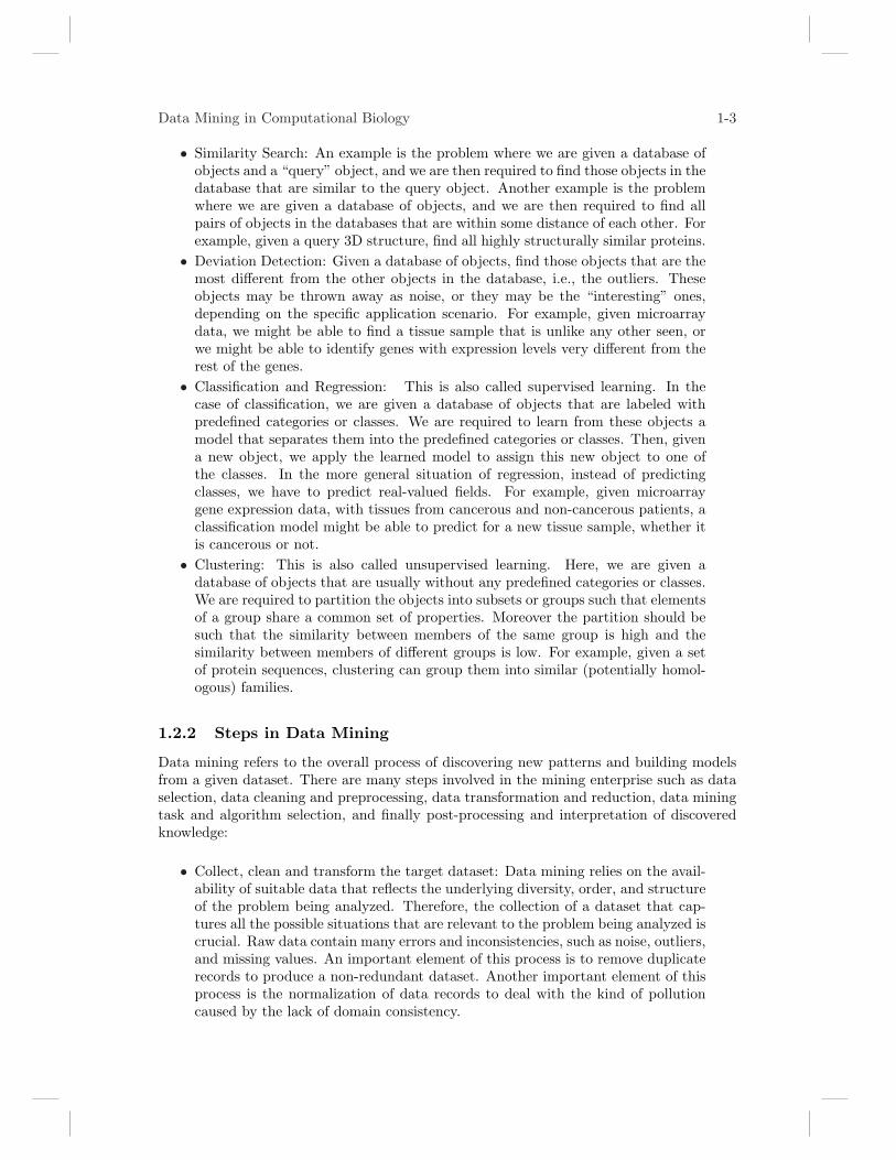
• Similarity Search: An example is the problem where we are given a database ofobjects and a “query” object, and we are then required to find those objects in thedatabase that are similar to the query object. Another example is the problemwhere we are given a database of objects, and we are then required to find allpairs of objects in the databases that are within some distance of each other. Forexample, given a query 3D structure, find all highly structurally similar proteins.

• Deviation Detection: Given a database of objects, find those objects that are themost different from the other objects in the database, i.e., the outliers. Theseobjects may be thrown away as noise, or they may be the “interesting” ones,depending on the specific application scenario. For example, given microarraydata, we might be able to find a tissue sample that is unlike any other seen, orwe might be able to identify genes with expression levels very different from therest of the genes.

• Classification and Regression: This is also called supervised learning. In thecase of classification, we are given a database of objects that are labeled withpredefined categories or classes. We are required to learn from these objects amodel that separates them into the predefined categories or classes. Then, givena new object, we apply the learned model to assign this new object to one ofthe classes. In the more general situation of regression, instead of predictingclasses, we have to predict real-valued fields. For example, given microarraygene expression data, with tissues from cancerous and non-cancerous patients, aclassification model might be able to predict for a new tissue sample, whether itis cancerous or not.

• Clustering: This is also called unsupervised learning. Here, we are given adatabase of objects that are usually without any predefined categories or classes.We are required to partition the objects into subsets or groups such that elementsof a group share a common set of properties. Moreover the partition should besuch that the similarity between members of the same group is high and thesimilarity between members of different groups is low. For example, given a setof protein sequences, clustering can group them into similar (potentially homol-ogous) families.

1.2.2 Steps in Data Mining

Data mining refers to the overall process of discovering new patterns and building modelsfrom a given dataset. There are many steps involved in the mining enterprise such as dataselection, data cleaning and preprocessing, data transformation and reduction, data miningtask and algorithm selection, and finally post-processing and interpretation of discoveredknowledge:

• Collect, clean and transform the target dataset: Data mining relies on the avail-ability of suitable data that reflects the underlying diversity, order, and structureof the problem being analyzed. Therefore, the collection of a dataset that cap-tures all the possible situations that are relevant to the problem being analyzed iscrucial. Raw data contain many errors and inconsistencies, such as noise, outliers,and missing values. An important element of this process is to remove duplicaterecords to produce a non-redundant dataset. Another important element of thisprocess is the normalization of data records to deal with the kind of pollutioncaused by the lack of domain consistency.

1-4

• Select features, reduce dimensions: Even after the data have been cleaned up interms of eliminating duplicates, inconsistencies, missing values, and so on, theremay still be noise that is irrelevant to the problem being analyzed. These noiseattributes may confuse subsequent data mining steps, produce irrelevant rulesand associations, and increase computational cost. It is therefore wise to performa dimension reduction or feature selection step to separate those attributes thatare pertinent from those that are irrelevant.

• Apply mining algorithms and interpret results: After performing the pre-processingsteps apply appropriate data mining algorithms—association rule discovery, se-quence mining, classification tree induction, clustering, and so on—to analyzethe data. After the algorithms have produced their output, it is still necessaryto examine the output in order to interpret and evaluate the extracted patterns,rules, and models. It is only by this interpretation and evaluation process thatwe can derive new insights on the problem being analyzed.

1.3 Mining 3D Protein Data

Protein structure data has been mined to extract structural motifs [29, 22, 31], analyzeprotein-protein interactions [55], protein folding [65, 39], protein thermodynamic stabil-ity [5, 38], and many other problems. Mining structurally conserved motifs in proteins isextremely important, as it reveals important information about protein structure and func-tion. Common structural fragments of various sizes have fixed 3D arrangements of residuesthat may correspond to active sites or other functionally relevant features, such as Prositepatterns. Identifying such spatial motifs in an automated and efficient way, may have agreat impact on protein classification [13, 3], protein function prediction [20] and proteinfolding [39]. We first describe in detail a graph-based method for mining structural motifs,and then review other approaches.

1.3.1 Modeling Protein Data as a Graph

An undirected graph G(V,E) is a structure that consists of a set of vertices V = {v1, · · · , vn}and a set of edges E ⊆ V ×V , given as E = {ei = (vi, vj)|vi, vj ∈ V }, i.e., each edge ei is anunordered pair of vertices. A weighted graph is a graph with an associated weight functionW : E → <+ for the edge set. For each edge e ∈ E, W (e) is called the weight of the edge e.Protein data is generally modeled as a connected weighted graph where each vertex in thegraph may correspond to either a secondary structure element (SSE) (such as α-helix orβ-strand) [22, 66], or an amino acid [29], or even an individual atom [31]. The granularitypresents a trade-off between computation time and complexity of patterns mined; a coarsegraph affords a smaller problem computationally, but runs the risk of oversimplifying theanalysis. An edge may be drawn between nodes/vertices indicating proximity, based onseveral criteria, such as:

• Contact Distance (CD) [29, 66]: Given two amino acids ai and aj along with the3D co-ordinates of their α-Carbon atoms (or alternately β-Carbon), (xi, yi, zi)and (xj , yj , zj), resp., define the Euclidean distance between them as follows:

δ(ai, aj) =√

(xi − xj)2 + (yi − yj)2 + (zi − zj)2

We say that ai and aj are in contact, if δ(ai, aj) ≤ δmax, where δmax is somemaximum allowed distance threshold (a common value is δmax = 7A). We can

Data Mining in Computational Biology 1-5

add an edge between two amino acids if there are in contact. If the vertices areSSEs then the weight on an edge can denote the number of contacts between thetwo corresponding SSEs.

• Delaunay Tessellation (DT)[29, 54, 62]: the Voronoi cell of x ∈ V (G) is given by

V(x) = {y ∈ <3|d(x, y) ≤ d(x′, y) ∀x′ ∈ V (G)\{x}}An edge connects two vertices if their Voronoi cells share a common face.

• Almost Delaunay (AD) [29]: to accommodate for errors in the co-ordinate valuesof the points in the protein structure data, we say that a pair of points vi, vj ∈V (G) are joined by an almost-Delaunay edge with parameter ε, or AD(ε), if byperturbing all points by at most ε, vi, vj could be made to have Voronoi cellssharing a face.

1.3.2 Graph-based Structural Motif Mining

(a) 2IGD Structure (b) 2IGD Graph

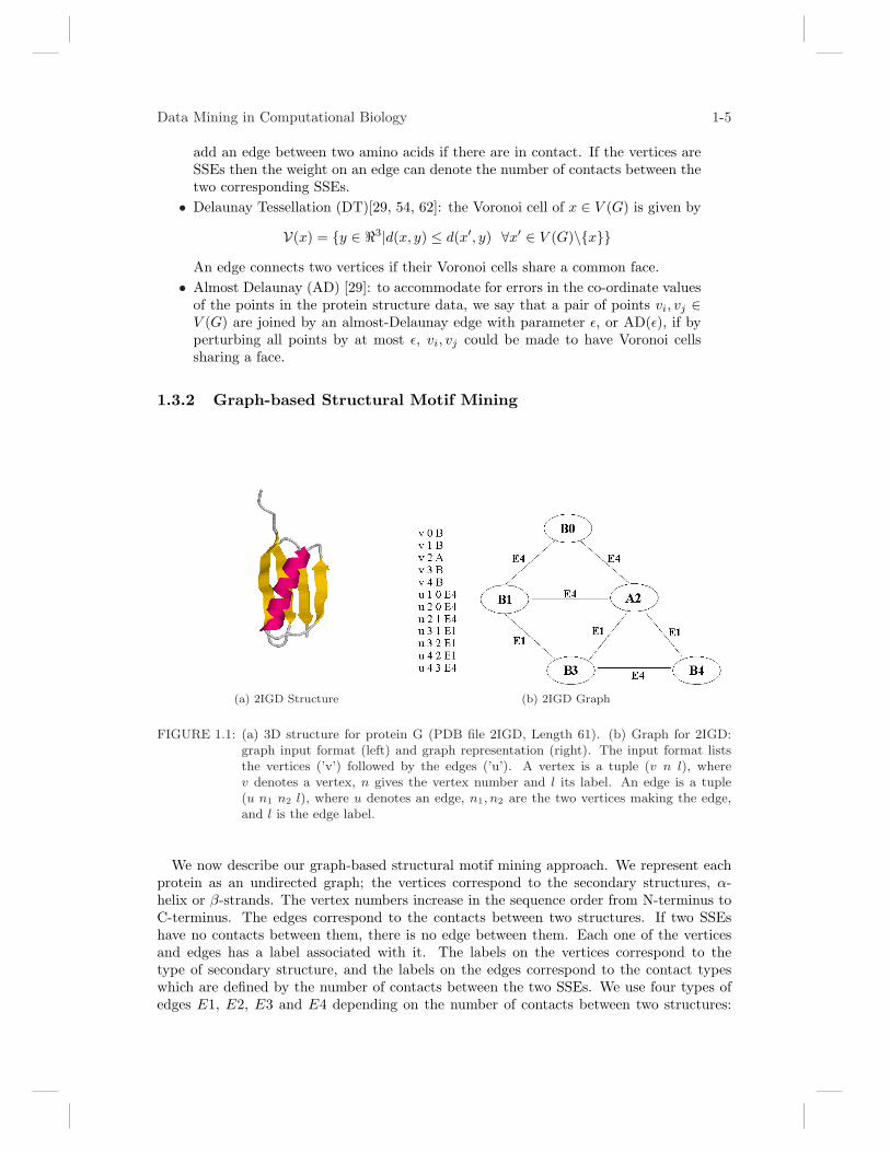
FIGURE 1.1: (a) 3D structure for protein G (PDB file 2IGD, Length 61). (b) Graph for 2IGD:graph input format (left) and graph representation (right). The input format liststhe vertices (’v’) followed by the edges (’u’). A vertex is a tuple (v n l), wherev denotes a vertex, n gives the vertex number and l its label. An edge is a tuple(u n1 n2 l), where u denotes an edge, n1, n2 are the two vertices making the edge,and l is the edge label.

We now describe our graph-based structural motif mining approach. We represent eachprotein as an undirected graph; the vertices correspond to the secondary structures, α-helix or β-strands. The vertex numbers increase in the sequence order from N-terminus toC-terminus. The edges correspond to the contacts between two structures. If two SSEshave no contacts between them, there is no edge between them. Each one of the verticesand edges has a label associated with it. The labels on the vertices correspond to thetype of secondary structure, and the labels on the edges correspond to the contact typeswhich are defined by the number of contacts between the two SSEs. We use four types ofedges E1, E2, E3 and E4 depending on the number of contacts between two structures:

1-6

E1 ∈ [1, 5), E2 ∈ [5, 10), E3 ∈ [10, 15), E4 ∈ [15, +∞). The graph representation of theprotein 2IGD with contact cutoff 7A is shown in Figure 1.1. There are 5 secondary structuresin 2igd: β0, β1, α2, β3, β4 and 7 edges between β1−β0, α2−β0, α2−β1, β3−β1, β3−β2,β4− β2, and β4− β3.

Discovering Frequent Subgraphs

To mine the frequent structural motifs from the database of proteins represented as graphswe used the FSG algorithm for frequent subgraph discovery[44]. The input is a databaseD of protein graphs and a minimum support threshold σ. The output is the set of allconnected subgraphs that occur in at least σ% of the proteins.

There are three considerations when FSG are applied to the database of protein struc-tures. Firstly, we are interested in subgraphs that are composed of all secondary structuresin contact, whether or not they are consecutive. A protein sequence or subsequence isnaturally connected from N -terminal to C-terminal, thus any two successive structuresare connected with each other. Contacts between two non-successive structures can formtertiary structure as well. Secondly, we used labeled graphs, where different graphs cancontain vertices and edges with the same label. We classified edges in four types accordingto the range of contacts. We chose this classification range heuristically to allow us to findpatterns containing multiple occurrences of the same structures and contact ranges. A finerclassification of edge types will decrease the frequency of common patterns and make therunning time extremely slow. Thirdly, we are interested in the subgraphs with at least σ%frequency in the database. This makes sure that the generated subgraphs are the dominantmotifs.

FSG uses a level-by-level approach to mine the connected subgraphs. It starts with thesingle edges and counts their frequency. Those that meet the support threshold are extendedby another frequent edge to obtain a set of candidate edge pairs. The counting proceedsby extending a frequent edge-set by one more edge. The process stops when no frequentextension is possible. For a detailed description of FSG see [44].

We ran the FSG algorithm on a dataset of 757 protein graphs obtained from the non-redundant proteins in PDBselect database [27]. The results with different frequency thresh-olds ranging from 10% to 40%, and with contact cutoff 7A are shown in Table 1.2. Figure 1.3shows some mined subgraphs with different number of edges using support 10%.

We mapped the mined graph patterns back to the PDB structure to visualize the minedresults. Two such frequent tertiary motifs are shown in Figure 1.4. The top one has 6edges, and frequency 157. This motif shows four alpha helices and three beta strands.Two proteins where this pattern occurs are also shown: PDB files 1AD2 and 1KUH. Thebottom motif has 8 edges and frequency 153. It is an all alpha motif. Two occurrences inPDB files 1BG8 and 1ARV are shown. The results obtained from graph mining are quiteencouraging. We found that most of the highest scoring patterns match part of the wholeprotein structures, and we were able to find remote interactions as well.

Comparison with SCOP Database

The SCOP protein database[50], categorizes proteins into all-α, all-β, α and β (inter-spersed), α plus β (isolated), and multi-domain according to their structure and functionalsimilarity. We applied the graph-mining method to protein families classified in SCOPdatabase. In order to find out whether our method matches with SCOP in mining andcategorizing common domains, several protein families were chosen randomly from SCOPand represented as graphs. Within one protein family, we used 100% support to find thelargest frequent patterns that appear in every protein in that family.

Data Mining in Computational Biology 1-7

10% 20% 30% 40%1-edge graphs 12 10 8 42-edges graphs 34 23 8 63-edges graphs 144 42 17 64-edges graphs 420 72 22 25-edges graphs 1198 142 23 06-edges graphs 2920 289 4 07-edges graphs 6816 32 0 08-edges graphs 14935 114 0 0

FIGURE 1.2: Frequent subgraphs

FIGURE 1.3: Highest Frequency Tertiary Motifs:Edge Size 1 to 8. The notation “t #1, 523” inthe graph input format denotes edge size = 1, support = 523.

FIGURE 1.4: Top: Alpha-Beta Motif and its Occurrence in PDB files: 1ad2, 1kuh. Bottom: AllAlpha Motif and its Occurrence in PDB files: 1bg8, 1arv

1-8

FIGURE 1.5: Largest pattern in 100% of DNA polymerase processivity factor proteins

(a) 1PLQ (b) 1CE8 (c) 1CZD

FIGURE 1.6: Some occurrences of the pattern in PDB files: 1PLQ, 1CE8, 1CZD

To test retrieval rate, we can create a mixed database from several families within the samesuperfamily. Mining this database, frequent patterns, could only be found with less than100% support. If we add to the database some other proteins outside of the superfamily,the maximum size pattern was only found at very small support and it is not frequentany more. This demonstrates that our graph mining method could be used to classifyproteins into families based on their shared motifs. For example, consider the DNA clampsuperfamily, which is made up of two families: DNA polymerase III, beta subunit and DNApolymerase processivity factor. DNA polymerase III beta subunit family has three E. coliproteins: 2POL, 1JQL and 1JQJ. The DNA polymerase processivity factors family has eightproteins: Bacteriophage RB69 (1B77, 1B8H) and Bacteriophage T4 (1CZD), human herpesvirus type 1 (1DML), proliferating cell nuclear antigens (1PLQ, 1PLR, 1AXC, 1GE8). Thefollowing pattern, shown in Figure 1.5 and its corresponding occurrences in PDB files,shown in Figure 1.6, appears in every protein of DNA polymerase processivity factors. Thegraph-based method has the potential to become a powerful tool in structure analysis. Itis a rapid, intuitive method to identify and find proteins that display structure similaritiesat the level of residues and secondary structure elements.

1.3.3 Alternate Approaches for Structural Motif Mining

Another graph based approach to motif discovery was proposed in [29], where they searchfor frequent subgraphs in proteins belonging to the same structural and functional familyin the SCOP database; they propose these subgraphs as family-specific amino acid residue

Data Mining in Computational Biology 1-9

signatures of the underlying family. They represent the protein structures as graphs, usingCD, DT and AD representations (see section 1.3.1). They represent each protein graph byan adjacency matrix in which each entry is either a 0 (if there is no edge), a vertex label(if it is a diagonal element), or an edge label (if an edge exists). They define the code ofthis adjacency matrix as the sequence of the entries in the lower triangular matrix readgoing left to right and then top to bottom. They use the lexicographic order to impose anordering on the codes obtained by rearranging the rows of the matrix. Using a novel graphrepresentation such as this, they construct a rooted, ordered tree for each graph and thensearch for frequent graphs. They then discard those which have a low mutual informationscore. They conclude that in order to achieve the highest accuracy in finding proteinfamily specific signatures, AD graphs present the best choice both due to their relativecomputational efficiency and their robustness in taking into account possible experimentalerrors in determining protein atomic coordinates.

In a different approach, Jonassen et al. [35] represent the neighborhood of each residue ras a neighbor string NSr of which r is called the anchor. NSr encodes all residues within ad angstrom radius of r. Each residue is encoded by its amino acid type, secondary structuretype and a coordinate set (x, y, z) calculated as the mean of the r’s side chain atoms. Theorder of residues in NSr is governed by their order along the protein’s backbone. They thendefine a packing pattern against which the neighbor strings are matched. A packing patternconsists of a list of elements where each element defines a match set (a set of allowed aminoacids), a set of allowed SSE types and one set of coordinates. NSr = r1, . . . , rk, . . . , rl,where rk is the anchor residue, is said to match packing pattern P = p1, . . . , pl, . . . , pn ifNSr contains a subsequence ri1, . . . , rin, such that residues have amino acids and SSE typesincluded in the match sets of the corresponding pattern elements and the anchors of theneighbor string and pattern string are aligned. Also, NSr is said to structurally match Pwithin φ, if it is possible to superimpose the coordinates of NSr onto those of P with aroot mean square deviation of maximum φ. A neighbor string that structurally matchesa packing pattern with a threshold φ describes an occurrence of the pattern. A patternhaving occurrences in k structures is said to have support k. Thus, they seek packingpatterns having support k in a dataset of N structures. For each of the N structures, apacking pattern is generated for the generalization of each neighbor string. There may existmany generalizations of the match sets and hence pruning based on geometrical constraintsis used to constrain the length of the neighbor strings. The packing pattern inherits itscoordinates and SSE types from the neighbor string. Further, neighbor strings with fewerthan 4 elements are discarded. Using depth-first search, they search for all generalizationsof a neighbor string having support k moving from simple (short generalizations) to complex(long ones) as the depth of the search increases. For every pattern thus found, they computea score measuring the pattern’s information content divided by its maximum root meansquare deviation.

The 3D conformation of a protein may be compactly represented in a symmetrical, square,boolean matrix of pairwise, inter-residue contacts, or “contact map”. The contact mapprovides a host of useful information about the protein’s structure. In [28] Hu et al. describehow data mining can be used to extract valuable information from contact maps. Forexample, clusters of contacts represent certain secondary structures, and also capture non-local interactions, giving clues to the tertiary structure. They focus on two main tasks: 1)Given the database of protein sequences, discover an extensive set of non-local (frequent)dense patterns in their contact maps, and compile a library of such non-local interactions.2) Cluster these patterns based on their similarities and evaluate the clustering quality. Toenumerate all the frequent dense patterns they scan the database of contact maps with a2D sliding window of a user specified size W × W . Across all proteins in the database,

1-10

any sub-matrix under the window that has a minimum “density” (the number of contacts)is captured. The main complexity of the method stems from the fact that there can be ahuge number of candidate windows. Of these windows only relatively few will be dense,since the number of contacts is a lot less than the number of non-contacts. They propose afast hash-based approach to counting the frequency of all dense patterns. Finally they useagglomerative clustering to group the mined dense patterns to find the dominant non-localinteractions.

Several methods for secondary level motif finding have also been proposed. SPASMcan find the motifs consisting of arbitrary main-chain and/or side-chains in a proteindatabase[40]. An algorithm based on subgraph isomorphism was proposed in[49]; it searchesfor an exact match of a specific pattern in a database. Search for distantly related proteinsusing a graph to represent the helices and strands was proposed in[42]. An approach basedon maximally common substructures between two proteins was proposed in[23]; it also high-lights areas of structural overlap between proteins. SUBDUE [15] is an approach based onMinimum Description Length and inexact graph matching for finding patterns in proteins.Another graph based method for structure discovery, based on geometric hashing, was pre-sented in [61]. Most of these methods either focus on identifying predefined patterns in agroup of proteins, or find approximate/inexact matches.

1.3.4 Finding Sites of Non-bonded Interaction

Sites of non-bonded interaction are extremely important to find, as they cannot be deter-mined from primary structure and give clues about the higher-order structure of the protein.Side chain clusters in proteins aid in protein folding and in stabilizing the three-dimensionalstructure of proteins [25]. Also, these sites may be occurring in structurally similar proteinswith very low sequence homology [37]. Spectral methods have been gaining favor in findingclusters of non-bonded interaction as they use global information of non-bonded interactionsin the protein molecule to identify clusters.

In [11], Brinda et al. construct a graph, where each vertex is a residue and they connectvertices if they are in contact (using cut-off 4.5A). They represent the protein graph interms of an adjacency matrix A, where ap,q = 1/dp,q, if p, q ∈ V (G) are connected and1/100, otherwise, dp,q = distance between p and q. The degree matrix, D, is a diagonalmatrix obtained by summing up the elements of each column. Then, the Laplacian matrix,L = D − A, is of dimension |V | × |V |. Using eigen decomposition on L, they get theeigenvalues and the eigenvectors. The Fiedler eigenvector, corresponding to the secondlowest eigenvalue, gives the clustering information [24]. The centers of the clusters canbe identified from the eigenvectors of the top eigenvalues. The cluster centers identifiedcorrespond to the nodes with the highest connectivity (degree) in the cluster, which generallycorrespond to the geometric center of the cluster. They consider clusters with at least threeresidues. The residues with the same vector component in the second lowest eigenvalueform a cluster. The residue with the highest magnitude of a vector component in thecorresponding top eigenvalue is the center of the cluster.

The α/β barrel proteins are known to adopt the same fold in spite of very low sequencesimilarity. This could be possible only if the specific stabilizing interactions important inmaintaining the fold are conserved in topologically equivalent positions. Such stabilizationcenters are usually identified by determining the extent of long-range contacts made by theresidue in the native structure. In [36], Kannan et al. use a data set of 36 (α/β) barrelproteins having average pair-wise sequence identity less than 10%. They represent eachprotein by a connected graph using contact distance approach to connect vertices/residueswith δ = 6.5A. The representation chosen causes high connectivity among the vertices of

Data Mining in Computational Biology 1-11

the graph and hence operating on the Laplacian of the graph is ineffective. Hence theyoperate on the adjacency matrix corresponding to the proteins. On eigen decomposition,they get a set of eigenvalue-eigenvector pairs. They sort this set based on the eigenvalues.They consider the set of largest eigenvalue-eigenvector pairs. Those residues having a largevector component magnitude in the direction of any of these eigenvectors are believed tobelong to the cluster corresponding to that eigenvector. Thus, they cluster the residues.In each cluster, the residue having largest vector component magnitude in the direction ofthe corresponding eigenvector is the center of that cluster. Using eigenvalue analysis, theyinfer the degree of each vertex. The residues with the largest degree (typically the clustercenters) correspond to the stabilization centers. They found that most of the residuesgrouped in clusters corresponding to the higher eigenvalues, typically occur in the strandregions forming the β barrel and were found to be topologically conserved in all 36 proteinsstudied.

1.4 Mining Microarray Gene Expression Data

High-throughput gene expression has become an important tool to study transcriptionalactivity in a variety of biological samples. To interpret experimental data, the extent anddiversity of gene expression for the system under study should be well characterized. Amicroarray [59] is a small chip (made of chemically coated glass, nylon membrane or silicon),containing a (usually rectangular) grid into which tens of thousands of DNA molecules(probes) are attached. Each cell of the grid relates to a fragment of DNA sequence.

Typically, two mRNA samples (a test sample and a control sample) are reverse-transcribedinto cDNA (targets) and labeled using either fluorescent dyes or radioactive isotopes. Theyare then hybridized by base-pairing, with the probes on the surface of the chip. The chipis then scanned to read the signal intensity that is emitted from the labeled and hybridizedtargets. The ratio of the signal intensity emitted from the test target to that emitted fromthe control target is a measure of the gene expressivity of the test target with respect tothe control target.

Typically, each row in the microarray grid corresponds to a single gene and each column,to either an experiment the gene is subjected to, or a patient the gene is taken from. Thecorresponding gene expression values can be represented as a matrix of real values where theentry (i, j) corresponds to the gene expression value for gene i under experiment j or frompatient j. Formally, the dataset is represented as Y = {y(i, j) ∈ <+|1 ≤ i ≤ n, 1 ≤ j ≤ m}where n,m are the number of rows(genes) and columns(experiments) and <+ is the set ofpositive real numbers. We represent the vector of expression values corresponding to gene iby y(i, · ) and that corresponding to experiment/patient j by y(· , j). A microarray datasetis typically tens of thousands of rows (genes) long and as many as one hundred columns(experiments/patients) wide. It is also possible to think of microarray data as the transposeof Y, i.e., where the rows are experiments and the columns are genes.

The typical objectives of a microarray experiment is to:

1. Identify candidate genes or pathological pathways: We can conduct a microarrayexperiment, where the control sample is from a normal tissue while the testsample is from a disease tissue. The over-expressed or under-expressed genesidentified in such an experiment may be relevant to the disease. Alternatively, agene A, whose function is unknown, may be similarly expressed with respect toanother gene B, whose function is known. This may indicate A has a functionsimilar to that of B.

1-12

2. Discovery and prediction of disease classes: We can conduct a microarray exper-iment using genes from patients known to be afflicted with a particular diseaseand cluster their corresponding gene expression data to discover previously un-known classes or stages of the disease. This can aid in disease detection andtreatment.

1.4.1 Challenges of Mining Microarray Data

One of the main challenges of mining microarray data is the high dimensionality of thedataset. This is due to the inherent sparsity of high-dimensional space. It has been proven[8], that under certain reasonable assumptions on the data distribution and for a variety ofdistance functions, the ratio of the distances of the nearest and farthest points to a givenpoint in a high-dimensional dataset, is almost 1. The process of finding the nearest pointto a given point is instrumental in the success of algorithms, used to achieve the objectivesmentioned above. For example, in clustering, it is imperative that there is an acceptablecontrast in distances between points within the same cluster and distances between pointsin different clusters.

Another difficulty in mining microarray data arises from the fact that there are oftenmissing or corrupted values in the microarray matrix, due to problems in hybridization orin reading the expression values. Finally, microarray data is very noisy. A large number ofthe genes or experiments may not contribute any interesting information, but their presencein the dataset makes detection of subtle clusters and patterns harder and increases themotivation for highly scalable algorithms.

1.4.2 Association Rule Mining

In order to achieve the objective of discovery of candidate genes in pathological pathways,there has been an attempt to use association rules [2]. Association rules can describe howthe expression of one gene may be associated with the expression of a set of genes. Giventhat such an association exists, one might easily infer that the genes involved participate insome type of gene network.

In order to apply association mining, it is necessary that the data be nominal. In[16], Creighton et al. first discretize the microarray data, so that each y(a, b) is set to{high, low, moderate} depending on whether it is up-regulated, down-regulated and nei-ther considerably up nor down regulated, respectively. Then, the data corresponding toeach experiment, i.e., (y(· , a)) can be thought of as a transaction from the market-basketviewpoint. They then apply the standard Apriori algorithm to find the association rulesbetween the different genes and their expression levels. This yields rules of the formg1(↑) ∧ g3(↓) ⇒ g2(↑), which means that if gene g1 is highly expressed and g3 is under-expressed, then g2 is over-expressed. Such expression rules can provide useful insight intothe expression networks.

1.4.3 Clustering Algorithms

In order to achieve the objective of discovery of disease classes, there are three types ofclustering algorithms:

1. Gene-based clustering: the dataset is partitioned into groups of genes havingsimilar expression values across all the patients/experiments.

Data Mining in Computational Biology 1-13

2. Experiment-based clustering: the dataset is partitioned into groups of experi-ments having similar expression values across all the genes.

3. Subspace clustering: the dataset is partitioned into groups of genes and experi-ments having similar expression values.

If the algorithm searches for clusters, which have elements which are similar across alldimensions, it can be called a “full dimensional” one.

Similarity Measures

Before delving into the specific clustering algorithms used, we must discuss the measuresused to express similarity between the expression values. Although, formulae mentionedin this section describe similarity between rows of the gene expression matrix, they can,without loss of generality be applied, to describe similarity between the columns of the geneexpression matrix as well.

One of the most used classes of distance metrics is the Lp distance where

||y(a, · )− y(b, · )||p∈<+ =

(m∑

t=1

|y(a, t)− y(b, t)|p)1/p

In this family, the L1, L2 and L∞ metrics, also called the Manhattan, Euclidean and Cheby-shev distance metrics, respectively, are the most studied; the Euclidean distance metric isthe most commonly used [21, 47, 12]. However, these measures do not perform too wellin high-dimensional spaces. Note that this class of metrics treats all dimensions equally,irrespective of their distribution. This is remedied to some extent, by standardizing thedata, i.e. normalizing the data in each row to the range [0,1] having mean 0 and standarddeviation 1 [17, 58]. Note that standardization assumes the underlying data is multivariatenormal.

Alternatively, researchers [18, 19, 12, 63] have used Pearson’s correlation coefficient as asimilarity measure, where

r(y(a, · ), y(b, · )) =∑m

t=1(y(a, t)− µ(y(a, · )))(y(b, t)− µ(y(b, · )))√(∑m

t=1(y(a, t)− µ(y(a, · )))2)(∑mt=1(y(b, t)− µ(y(b, · )))2)

where µ(y(a, · )) =∑m

t=1y(a,t)

N and µ(y(b, · )) =∑m

t=1y(b,t)

N .Note that r assumes the two vectors are approximately normally distributed and jointly

bivariate normal. In this case there is a strong relationship between r and standardizedEuclidean distance, since if y(a, · ) and y(b, · ) are standardized,

||y(a, · )− y(b, · )||2 =√

2m(1− r(y(a, · ), y(b, · )))

If µ(y(a, · )) = µ(y(b, · )) = 0, i.e. the vectors are translated so their mean is 0, thenr is identical to the cosine similarity between the vectors, which is a similarity measureknown to be highly effective in high-dimensional spaces. Other distance measures tested inmicroarray data analysis include Kullback-Leibler distance or mutual information [47].

Gene-based Clustering

A number of traditional clustering algorithms like k-means [58] and hierarchical clustering[19] have been used to find full-dimensional clusters in microarray data.

1-14

K-means(Y,sim,k)1. select k points(genes) from Y randomly as cluster centers2. repeat until convergence3. for s=1 to n4. assign y(s, · ) to the cluster whose center is most similar to it using sim5. for j=1 to k6. recalculate center of cluster cj as mean of all rows(genes) assigned to it

The k-means algorithm, shown above, is a partitional, iterative clustering algorithm. Ittakes as input the n×m dataset Y, the similarity measure sim, and the number of clustersto mine k. K-means runs very quickly in O(nmt) time (t is the number of iterations, andk is a small constant), but suffers from the disadvantage that it requires a parameter k tobe supplied, indicating the number of clusters to be found. This parameter is hard to set.Also, k-means is highly sensitive to noise and outliers, because it assigns every point in thedataset to some cluster. K-means converges to a local optima and theoretical guarantees ofits accuracy are yet to be proven. The practical accuracy of k-means is noted to improveconsiderably, if the initial assignment of points to clusters is not so arbitrary [10].

A Self-Organizing Map (SOM)[43] is based on a single-layered neural network which mapsvectors(rows/genes) in the microarray data to a two-dimensional grid of output nodes. Eachinput node is a row from the microarray dataset and each output node corresponds to avector in the high-dimensional space.

SOM(Y,sim, k, g, r)1. select k vectors(genes) from Y randomly as output nodes2. repeat until convergence3. For s=1 to n4. find output node most similar to y(s, · ) using sim5. update all nodes in the r-neighborhood of that output node

As shown above, a SOM trains on the input microarray dataset to adjust its outputnodes (line 5), so that they move toward the denser regions of the high-dimensional featurespace. The algorithm uses a number of user-specified parameters like the learning rate (g)and the neighborhood size(r). Also, SOM converges slower than k-means but is far morerobust than k-means. SOM [56] and related algorithms [26] have been used for gene-basedclustering.

Hierarchical clustering has two flavors: agglomerative (bottom-up) and divisive (top-bottom). In agglomerative gene-based clustering (shown below), each gene is initiallyassigned to its own cluster (line 1). In each iteration the two clusters with the highestinter-cluster similarity (line 3) are merged to form a single one (line 4), until some con-vergence criterion is satisfied e.g., the desired number of clusters remain, only one clusterremains, etc. The inter-cluster similarity may be computed by a number of methods suchas:

• single linkage, where Sim(a,b) = maxi∈a,j∈b sim(i, j).• complete linkage, where Sim(a,b) = mini∈a,j∈b sim(i, j).

• average linkage, where Sim(a,b) =∑

i∈a,j∈bsim(i,j)

|a||b| .

• average group linkage, where Sim(a,b) =∑

i∈a∪b,j∈a∪bsim(i,j)

|a∪b|2 .

Data Mining in Computational Biology 1-15

Here Sim is the inter-cluster similarity of clusters a and b, each having |a| and |b| genesassigned to them respectively and sim is the similarity measure between two genes. Thismerging of clusters gives rise to a tree called a dendrogram. This algorithm is greedy andsusceptible to noise. Also, it has time complexity O(n2 log n) [32] implying it convergesslower than K-means.

Agglomerative(Y,Sim)1. Assign each y(1, · ), i ∈ [1, n] to its own cluster to form set of clusters C2. repeat until convergence3. {a∗,b∗} = argmin(a,b)∈C×CSim(a,b)4. a∗ = a∗ ∪ b∗,C = C\b∗

In divisive clustering, all the genes are initially assigned to the same cluster. Then itera-tively, one of the clusters is selected from those existing, and is split into two clusters basedon some splitting criterion. This continues, until some convergence criterion is achievede.g., each gene has its own cluster, desired number of clusters remain, etc.

Experiment-based Clustering

For experiment-based clustering, the dimensionality (i.e. the number of genes) of the spaceis extremely high. Solutions proposed to remedy the failure of distance metrics in suchhigh-dimensional spaces include, designing new distance metrics [1] and dimensionality re-duction [4, 52]. Dimension reduction techniques, such as the Karhunen-Loeve tranformation(KLT), and singular value decomposition (SVD) [4, 52] are applied as a preprocessing stepto reduce the number of dimensions prior to the application of a clustering algorithm. Insuch dimension reduction techniques, the entire database is projected onto a smaller set ofnew dimensions, called the principal components, which account for a large portion of thevariance in the dataset. These new dimensions are mutually uncorrelated and orthogonal.Each of them is a linear combination of the underlying dimensions. Once the data has beenprojected to a lower-dimensional space, any of the clustering algorithms can be applied.

Subspace Clustering

The strategy of dimension reduction using KLT may be inappropriate as the clusters in-volving the transformed dimensions may be hard to interpret for the user. Also, data isonly clustered in a single subspace. [2] cites an example, in which KLT does not reduce thedimensionality without trading off considerable information, as the dataset contains sub-sets of points which lie in different and sometimes overlapping lower dimensional subspaces.Hence, the focus of much recent microarray data analysis focuses on subspace clustering[6, 14, 21, 45, 57, 60, 63].

Ben-Dor et al.[6], seek to identify large order-preserving submatrices (OPSMs) in Y. Asubmatrix is order-preserving if there is a permutation of its columns under which thesequence of values in every row is strictly increasing. They prove that the problem is NP-hard. In that paper, they discuss two methods to discover clusters: a complete model anda partial model. The complete model is simply to enumerate every combination, which isunacceptable in reality. The partial model is a stochastic model.

Getz et al.[21] alternate between gene-based and experiment-based clustering. Theycluster using super-paramagnetic clustering (SPC), a divisive hierarchical clustering basedon the analogy to the physics of inhomogeneous ferromagnets [9], which is robust againstnoise and searches for “natural” stable clusters. They partition the microarray dataset into

1-16

gene-based and experiment-based clusters. The gene(experiment)-based clusters specify thegroup of genes(experiment) which are similar. They then cluster the set of genes reported byeach gene-based clustering over the set of experiments specified by each experiment-basedcluster. This continues until SPC clustering produces no new robust clusters.

Cheng et al.[14] proposed the biclustering algorithm which seeks to group subsets ofmicroarray data rows and columns having a high similarity score. They use the meansquared residue score as a similarity measure for a cluster. If O ⊆ [1, n], C ⊆ [1,m], themean square residue of (O,C) is defined as :

H(O,C) =1

|O||C|∑

i∈O,j∈C

(y(i, j)− µC(y(i, · ))− µO(y(· , j)) + µO,C(y(· , · )))

where, µC(y(i, · )) = 1|C|

∑j∈C y(i, j), µO(y(· , j) = 1

|O|∑

i∈O y(i, j), µO,C(y(· , · )) =1

|O||C|∑

i∈O,j∈C y(i, j). If H(O, C) ≤ δ, a user-specified threshold, the cluster (O,C) isretained. This definition imposes a constraint on the variation of gene expression values inthe genes in O across the experiments in C. Their algorithm aims to greedily find multipleδ-biclusters, one in each iteration. After discovering a cluster, the values in that cluster arereplaced by random data, so that partially overlapping biclusters may be found. However,if clusters naturally overlap, such random data may obstruct the detection of the overlap[60].

The p-clustering algorithm [60] is designed to solve this problem. Unlike biclustering, it isa deterministic algorithm. It defines a pScore of a 2×2 matrix X =

(a bc d

)as: pScore(X) =

|(a− b)− (c−d)|. A sub-matrix (O, C) is a δ-pCluster iff ∀X2×2 ∈ (O,C) pScore(X) ≤ δ, apredefined threshold. The intuition is that δ constrains the variation in the gene expressionvalues ((a − b), (c − d)), across the conditions (columns in X) over which the genes (rowsin X) cluster. They use the implicit recursivity in the definition of a δ-pCluster to designa depth-first algorithm that searches for maximal δ-pClusters. The pCluster algorithm candiscover every δ-pCluster in a data set, no matter whether the clusters are overlapping ornot. It has time complexity O(nm2log(n) + mn2log(m)).

1.5 Determining Normal Variation in Gene Expression Data

Having looked at the application of data mining to the problems of motif discovery andmicroarray gene expression analysis, we now highlight some issues in data pre-processing.We illustrate this with the problem of finding normal variation in gene expression data.

An ubiquitous and under-appreciated problem in microarray analysis is the incidence ofmicroarrays reporting non-equivalent levels of an mRNA or the expression of a gene for asystem under replicate experimental conditions. In ideal conditions, the gene expressionvalues for each gene should be the same across all array experiments. But due to thetechnical limitations the data contains lot of inherent noise, which could also be due tonormal variation in expression of the genes across the genetically identical male mice. Ourgoal is to extract those genes which are contributing to the noise due to their biologicalvariance. This kind of analysis should be done prior to mining, since otherwise, we mightcome to a wrong conclusion about co-expressed genes or genes that correlate well with apathological condition.

We try to capture the genes which show variance among the identical mice by trying toeliminate the variations which come in due to experimental errors and fluctuations. We usea very robust method to exclude genes, which would eliminate any considerable variance inthe replicates. Our approach is based on the following steps: 1) Calculation of fold-change

Data Mining in Computational Biology 1-17

ratio and discretization of expression levels for each gene, 2) Elimination of experimentalnoise, 3) Constructing an expression profile for each gene, and 4) Calculating and rakingby gene variability via entropy calculation. We describe the steps in more detail below.

1.5.1 Fold-Change Ratio

We assume that we have n genes, in m mice, with r replicates for each mice, for a giventissue. We denote gene i as gi. Let Si

t denote the expression level for gene gi in the testsample and Si

r the expression of gi in the reference microarray samples. We define fold-change ratio as the log-odds ratio of the expression intensities of the test sample over thereference sample, given as log2(

Sit

Sir). To analyze the variability, we discretize the fold-change

into k bins ranging from very low expression levels to very high expression levels. The datais normalized in such a way that the median of the deviation from the median was set tothe same value for the distribution of all the log-ratios on each array [51]. Similar analysiswas done for the Affymetrix data. The raw data containing the intensities was mediancentered and scaled by the standard deviation. This normalization technique was chosenafter experimenting with other methods like linear regression and mean centering. Thoughnone of these methods yielded a normal distribution for the histogram plot of the geneexpression values of all clones in a sample, the median centered normalization techniqueperformed the best and also provided a uniform distribution for our binning method.

Rep1 Rep2 Rep3 Rep4

Mouse1 {g1V H , g2

V L, g3V H , g4

L} {g1V H , g2

V L, g3V H , g4

N} {g1V H , g2

V L, g3V H , g4

N} {g1V H , g2

V L, g3V H , g4

N}Mouse2 {g1

V H , g2V L, g3

L, g4N} {g1

V H , g2V L, g3

L, g4N} {g1

V H , g2V L, g3

L, g4N} {g1

V H , g2V L, g3

H , g4N}

Mouse3 {g1V H , g2

N , g3V H , g4

N} {g1V H , g2

N , g3V H , g4

N} {g1V H , g2

N , g3V H , g4

N} {g1V H , g2

N , g3V H , g4

L}Mouse4 {g1

V H , g2N , g3

V L, g4L} {g1

V H , g2N , g3

V L, g4N} {g1

V H , g2N , g3

V L, g4N} {g1

V H , g2N , g3

V L, g4N}

Mouse5 {g1V H , g2

H , g3L, g4

L} {g1V H , g2

H , g3L, g4

L} {g1V H , g2

H , g3L, g4

L} {g1V H , g2

H , g3L, g4

L}Mouse6 {g1

V H , g2H , g3

V H , g4L} {g1

V H , g2H , g3

V H , g4L} {g1

V H , g2H , g3

V H , g4N} {g1

V H , g2H , g3

V H , g4N}

If the number of bins for expression level discretization is too small or too high, then itleads to problems in analysis. In coarse binning, the information about the values is ignored,and in a very fine binning, the patterns are lost. We tried several values of k and found thatk = 5 works well. The bin intervals are determined using the uniform frequency binningmethod. Other popular methods like discriminant discretization, boolean reasoning basedand entropy based discretization can be considered [48]. In frequency binning method wediscretized the relative expression (fold-change) into 5 levels depending on their expressionvalue. The values of -1.5, -0.5, 0, 0.5, and 1.5 for the fold change ratio were taken asthresholds for very low (VL), low (L), normal (N), high (H), and very high (VH) expression,respectively. That is, V L ∈ (−∞,−1.5], V ∈ (−1.5,−0.5], N ∈ (−0.5, 0.5), H ∈ [0.5, 1.5),and V H ∈ [1.5, +∞). We use the notation gi

e to denote the expression level for gene gi

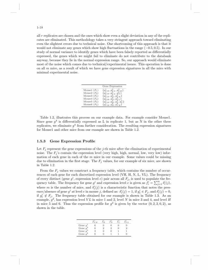
in a given replicate, where e ∈ {V L, L, N, H, V H}. Table 1.1 shows an example of theexpression of 4 genes in six mice with 4 array replicates for each mouse.

1.5.2 Elimination of Experimental Noise

In order to eliminate the noise due to experimental fluctuations, we process the data takingone mouse at a time. For each mouse the genetic expression signature is obtained and com-pared across all r replicates. Only those genes which show consistent expression signature in

1-18

all r replicates are chosen and the ones which show even a slight deviation in any of the repli-cates are eliminated. This methodology takes a very stringent approach toward eliminatingeven the slightest errors due to technical noise. One shortcoming of this approach is that itwould not eliminate any genes which show high fluctuations in the range (−0.5, 0.5). In ourstudy of normal variance to identify genes which have been falsely reported as differentiallyexpressed, the genes which we might fail to eliminate do not contribute to the databankanyway, because they lie in the normal expression range. So, our approach would eliminatemost of the noise which comes due to technical/experimental issues. This operation is doneon all m mice, as a result of which we have gene expression signatures in all the mice withminimal experimental noise.

Gene Expression

Mouse1 (F1) {g1V H , g2

V L, g3V H}

Mouse2 (F2) {g1V H , g2

V L, g4N}

Mouse3 (F3) {g1V H , g2

N , g3V H}

Mouse4 (F4) {g1V H , g2

N , g3V L}

Mouse5 (F5) {g1V H , g2

H , g3L, g4

L}Mouse6 (F6) {g1

V H , g2H , g3

V H}

Table 1.2, illustrates this process on our example data. For example consider Mouse1.Since gene g4 is differentially expressed as L in replicate 1, but as N in the other threereplicates, we eliminate g4 from further consideration. The resulting expression signaturesfor Mouse1 and other mice from our example are shown in Table 1.2.

1.5.3 Gene Expression Profile

Let Fj represent the gene expressions of the j-th mice after the elimination of experimentalnoise. The Fj ’s contain the expression level (very high, high, normal, low, very low) infor-mation of each gene in each of the m mice in our example. Some values could be missingdue to elimination in the first stage. The Fj values, for our example of six mice, are shownin Table 1.2.

From the Fj values we construct a frequency table, which contains the number of occur-rences of each gene for each discretized expression level (VH, H, N, L, VL). The frequencyof every distinct (gene gi, expression level e) pair across all Fj , is used to populate the fre-quency table. The frequency for gene gi and expression level e is given as f i

e =∑m

j=1 δie(j),

where m is the number of mice, and δie(j) is a characteristic function that notes the pres-

ence/absence of gene gi at level e in mouse j, defined as: δie(j) = 1, if gi

e ∈ Fj , and δie(j) = 0,

if gie 6∈ Fj . The frequency table obtained for our example is shown in Table 1.3. As an

example, g2, has expression level V L in mice 1 and 2, level N in mice 3 and 4, and level Hin mice 5 and 6. Thus the expression profile for g2 is given by the vector (0, 2, 2, 0, 2), asshown in the table.

fiV H fi

H fiN fi

L fiV L

Gene g1 6 0 0 0 0Gene g2 0 2 2 0 2Gene g3 3 0 0 1 1Gene g4 0 0 1 1 0

Data Mining in Computational Biology 1-19

1.5.4 Entropy-based Variability Ranking

The genes that show presence in more than one discrete level are of interest to us. Thefrequency table is analyzed further to identify those genes which show considerable varianceby their presence in more than one state. To capture the variance in a gene’s expressionlevel, the entropy measure was used. Entropy gives us the amount of disorder in theexpression values of a gene, and thus is a measure of the normal variance, since the noisedue to experimental variation is eliminated prior to this step. The entropy measure for agene gi is given as follows, E(gi) = −∑k

e=1 pie log2(pi

e), where k is the number of discreteexpression levels, and pi

e is the probability of gene gi having expression level e, which isgiven as pi

e = fie∑k

j=1fi

j

.

By definition of entropy, if a gene has only one expression level (say j), then pij = 1

and E(gi) = 0. On the other hand, if a gene has the most variance (i.e., equal occur-rence at each expression level), then P i

j = 1/k for all expression levels j, and E(gi) =−∑k

j=1 1/k log2(1/k) = − log2(1/k) = log2(k). In our approach genes with entropy 0, i.e.,those having no variance in expression across the mice, are discarded, and the remaininggenes are ranked in descending order of their entropy (and thus variance). The entropyranking for the four genes (along with the probability of each expression level) in our ex-ample are shown in Table 1.4. Gene g2 and g3 are of most interest to us because they showvariation in expression states across the six mice. On the other hand gene g1 is always highin all six mice, showing no variance.

piV H pi

H piN pi

L piV L Entropy

Gene g2 0 0.33 0.33 0 0.33 1.59Gene g3 0.6 0 0 0.2 0.2 1.37Gene g4 0 0 0.5 0.5 0 1Gene g1 1.0 0 0 0 0 0

1.5.5 Weighted Expression Profiles

In our approach to experimental noise elimination, any gene with varying expression levelamong the replicates is considered experimental noise, and eliminated. Instead of such astringent approach, we can choose to retain a gene provided it has the same expression levelin a given fraction of the replicates. For instance, gene g4 has expression level N in threeout of the four replicates for Mouse1. If we set our threshold to 75%, then we would retaing4

N in the gene expression for Mouse1 in Table 1.2.Another approach is to construct a weighted expression signature, as follows: For every

gene we record the fraction of the replicates in which it takes a particular value. Forinstance, for Mouse1, gene g1 always takes the value V H, so its weighted expression isg1

V H(1.0). On the other hand, gene g4 is N in three and L in one out of the four replicates;we record its weighted expression as g4

N(0.75),L(0.25). We denote by wie(j) the weight of gene

gi at expression level e in Mouse j. Table 1.5 shows the weighted expression signatures forall the six mice (note: if the weight is 1.0 we omit the weight; we write g1

V H instead ofg1

V H(1.0)).From the weighted gene expressions, we can construct a weighted profile using the ap-

proach in Section 1.5.3. The weighted frequency for gene gi and expression level e is given

1-20

Gene Expression

Mouse1 (F1) {g1V H , g2

V L, g3V H , g4

N(0.75),L(0.25)}Mouse2 (F2) {g1

V H , g2V L, g3

H(0.25),L(0.75), g4N}

Mouse3 (F3) {g1V H , g2

N , g3V H , g4

N(0.25),L(0.75)}Mouse4 (F4) {g1

V H , g2N , g3

V L, g4N(0.75),L(0.25)}

Mouse5 (F5) {g1V H , g2

H , g3L, g4

L}Mouse6 (F6) {g1

V H , g2H , g3

V H , g4N(0.5),L(0.5)}

as f ie =

∑mj=1 wi

e(j), where m is the number of mice. The weighted frequency table obtainedfor our example is shown in Table 1.6. As an example, g4, has expression levels N(0.75) inMouse1, N(1.0) in Mouse2, N(0.75) in Mouse3 and Mouse4, and N(0.5) in Mouse6. Thusf4

N = 0.75 + 1.0 + 2 × 0.75 + 0.5 = 3.75, and similarly f4L = 2.25. Thus the weighted

expression profile for g4 is given by the vector (0, 0, 3.75, 2.25, 0), as shown in the table.

fiV H fi

H fiN fi

L fiV L

Gene g1 6 0 0 0 0Gene g2 0 2 2 0 2Gene g3 3 0.25 0 1.75 1Gene g4 0 0 3.75 2.25 0

From the weighted expression profile, we can derive the entropy-based variability rankingfor each gene as shown in Table 1.7. Comparing with Table 1.4, we find that g3 is rankedhigher in terms of variability than g2, but the overall trend is similar.

piV H pi

H piN pi

L piV L Entropy

Gene g3 0.5 0.04 0 0.29 0.17 1.64Gene g2 0 0.33 0.33 0 0.33 1.59Gene g4 0 0 0.62 0.38 0 0.95Gene g1 1.0 0 0 0 0 0

1.5.6 Application Study

We applied our entropy-based method to detect normal variance in gene expression forthe two datasets taken from [51] and [46]. We used three datasets of kidney, liver andtestis provided by [51]. Six genetically identical male C57BL6 mice were used to comparethe expression values of 5,406 unique mouse genes. Four separate microarray assays wereconducted for each organ from each animal, for a total of 24 arrays per organ. Also thedataset of [46] was used which contained the expression values for three mice across thefour organs of liver, heart, lung and brain. Each experiment was replicated three times.Affymetrix oligo-chips were used in these experiments.

Using our entropy-based approach, in kidney tissue around 3.5% of the 3088 genes showedconsiderable variance across the six mice. As reported by [51] we found several immunemodulated and stress responsive genes. In liver tissue, 23 out of 2513 genes show significantvariation in their expression levels among the six mice. Out of the 3252 genes analyzed inthe testis tissue, 63 showed differential expression levels across the six mice. Importantly,

Data Mining in Computational Biology 1-21

many of the genes that we found to vary normally have been reported previously to bedifferentially expressed because of a pathological process or experimental intervention. Onerecent study used microarrays to investigate the differential gene expression patterns duringpre-implantation mouse development [41]. Rpl12 was reported to be differentially expressedwhile we found it to be normally varying in the testis tissue. PUFA (polyunsaturated fattyacids) feeding can influence Protein Kinase C (PKC) activity [7]. Itrp1 is another gene whichhas been reported as differentially expressed [30] in papillary thyroid carcinoma, while wefound this gene to be normally varying in kidney tissues. Another study investigated theeffects of acetaminophen on gene expression in the mouse liver [53]. Eight of the genesreported to differ in response to acetaminophen, including CisH2, and Hsp40, were geneswe found to vary normally.

Principal Component Analysis (PCA) [34] is a classical technique to reduce the dimen-sionality of the data set by transforming to a new set of variables (the principal components).It has been used in the analysis of gene expression studies. Principal components (PC’s)are uncorrelated and ordered such that the k-th PC has the k-th largest variance amongall PC’s. The k-th PC can be interpreted as the direction that maximizes the variation ofthe projections of the data points such that it is orthogonal to the first k − 1 PC’s. PCAis sometimes applied to reduce the dimensionality of the data set prior to clustering. UsingPCA prior to cluster analysis may aid better extraction of the cluster structure in the dataset. Since PC’s are uncorrelated and ordered, the first few PC’s, which contain most ofthe variations in the data, are usually used in cluster analysis. Unless external informationis available, [64] recommend cautious interpretation of any cluster structure observed inthe reduced dimensional subspace of the PC’s. They observe no clear trend between thenumber of principal components chosen and the cluster quality. [33] use PCA analysis forextracting tissue specific signatures.

We used PCA to analyze how well the genes we have extracted capture the normal vari-ance between the mice, eliminating the variance due to any other sources to the maximumpossible extent. Projection on to a 3-dimension space (the top three PCs) allows for bettervisualization of the entire data set. Figure 1.7 shows the arrangement of the samples byplotting them on the principal components derived from: 1) PCA analysis of all the genesin the dataset, and 2) PCA analysis of only those genes which were found to have normalvariance across mice. These plots are shown for all the three tissues under study. Kidneyand testis show non-random arrangement of the assay points while liver has less discerniblepatterns. In the case of the kidney tissue for genes with normal variance, the assays arrangeinto two clusters. One of the clusters has assays which include the replicates from four mice(M1, M2, M5, M6), while the other cluster has mice M3 and M4. This indicates that thereis a high similarity among these mice in kidney tissue. In the testis, the first two mice aresystematically different from the last four mice. No pattern was observed in liver. PCA canbe additionally used as a platform to compare the performance of different methodologiesto determine normal variance. The performance can be judged visually on the basis howwell the replicates cluster together or measure the goodness of the clusters. We observethat 1) the experimental replicates belonging to any single mice cluster close to each other,and 2) the mice (biological replicates) are also grouped into visible clusters. Pathologicallysimilar mice are clustered together.

1.6 Summary

The goal of this chapter was to provide a brief introduction to some data mining tech-niques, and to look at how data mining has been used in some representative applications

1-22

Kidney (All Genes)

M1M2M3M4M5M6

-15-10-50510

PC2 -10-5

05

1015

2025

PC1

-8-6-4-202468

1012

PC3

Kidney (Varying Genes)

M1M2M3M4M5M6

-4-3-2-10123

PC2 -4-3-2-10 1 2 3 4 5 6

PC1

-2.5-2

-1.5-1

-0.50

0.51

1.52

PC3

Testis (All Genes)

M1M2M3M4M5M6

-30-25-20-15-10-50510

PC2 -15-10

-50

510

15

PC1

-20

-15

-10

-5

0

5

10

PC3Testis (Varying Genes)

M1M2M3M4M5M6

-2-1.5-1-0.500.511.522.53

PC2 -5-4

-3-2

-10

12

3

PC1

-2

-1.5

-1

-0.5

0

0.5

1

1.5

2

PC3

Liver (All Genes)

M1M2M3M4M5M6

-20-15-10-5051015

PC2 -10-5

05

1015

2025

PC1

-10-8-6-4-202468

1012

PC3Liver (Varying Genes)

M1M2M3M4M5M6

-2.5-2-1.5-1-0.500.511.52

PC2 -4-3

-2-1

01

23

PC1

-2-1.5

-1-0.5

00.5

11.5

22.5

PC3

FIGURE 1.7: Principal component analysis of all genes (left column) and genes with normal vari-ance (right column). Three tissues were studied: Kidney (top row), Testis (middlerow), and Liver (bottom row). Results for all 6 mice and 4 replicates are shown

in bioinformatics, namely three-dimensional (3D) or structural motif mining in proteinsand the analysis of microarray gene expression data. We also looked at some issues in datapreparation, namely data cleaning and feature selection via the study of how to find normalvariation in gene expression datasets.

It is clear that data mining is playing a fundamental role in understanding the rapidlyexpanding sources of biological data. It is equally clear that new data mining techniques areneeded to analyze, manage and discover sequence, structure and functional patterns/modelsfrom large sequence and structural databases, as well as for structure prediction, genefinding, gene expression analysis, biochemical pathway mining, biomedical literature mining,drug design and other emerging problems in genomics and proteomics.

References 1-23

Acknowledgment

This work was supported in part by NSF CAREER Award IIS-0092978, DOE Career AwardDE-FG02-02ER25538, and NSF grant EIA-0103708. We thank Jingjing Hu and VinayNadimpally for work on contact map mining and determining normal variations in geneexpression data, respectively.

References

[1] C. Aggarwal. Towards systematic design of distance functions for data mining appli-cations. In 9th ACM SIGKDD Conference, 2003.

[2] R. Agrawal, J. Gehrke, D. Gunopulos, and P. Raghavan. Automatic subspace clusteringof high dimensional data for data mining applications. In ACM SIGMOD Conference,pages 94–105, 1998.

[3] N. Alexandrov and N. Go. Biological meaning, statistical significance and classificationof local spatial similarities in non-homologous proteins. Protein Sci., 3:866–875, 1994.

[4] O. Alter, P. Brown, and D. Botstein. Singular value decomposition for genome-wideexpression data processing and modeling. Proceedings of the National Academy ofSciences, 97:10101–10106, 2000.

[5] I. Bahar, A. Atilgan, and B. Erman. Direct evaluation of thermal fluctuations inproteins using a single parameter harmonic potential. Folding and Design, 2:173–181,1997.

[6] A. Ben-Dor, B. Chor, R. Karp, and Z. Yakhini. Discovering local structure in gene ex-pression data: The order-preserving submatrix problem. In 6th Annual InternationalConference on RECOMB, pages 49–57, 2002.

[7] A. Berger, D.M. Mutch, J. Bruce, G. Matthew, and A. Roberts. Dietary effects ofarachidonate-rich fungal oil and fish oil on murine hepatic and hippocampal geneexpression. Lipids in Health and Disease, 1:2–10, 2002.

[8] K. Beyer, J. Goldstein, R. Ramakrishnan, and U. Shaft. When is nearest neighborsmeaningful? In ICDT Conference, 1999.

[9] M. Blatt, S. Wiseman, and E. Domany. Data clustering using a model granular magnet.Neural Computation, 9:1805–1842, 1997.

[10] P. Bradley and U. Fayyad. Refining initial points for kmeans clustering. In 15thInternational Conference on Machine Learning, pages 91–99. Morgan Kaufmann,1998.

[11] K. Brinda, N. Kannan, and S. Vishveshwara. Analysis of homodimeric protein inter-faces by graph-spectral methods. Protein Engineering, 15:265–77, April 2002.

[12] Tang C., Zhang L., Zhang A., and Ramanathan M. Interrelated two-way clustering: Anunsupervised approach for gene expression data analysis. In 2nd IEEE InternationalSymposium on Bioinformatics and Bioengineering, pages 41–48, November 2001.

[13] S. Chakraborty and S. Biswas. Approximation algorithms for 3-d common substructureidentification in drug and protein molecules. In Workshop on Algorithms and DataStructures, pages 253–264, 1999.

[14] Y. Cheng and G. Church. Biclustering of expression data. In 8th InternationalConference on Intelligent Systems for Molecular Biology, volume 8, pages 93–103,2000.

[15] D.J. Cook, L.B. Holder, R. Maglothin S. Su, and I. Jonyer. Structural mining of

1-24 References

molecular biology data. IEEE Engineering in Medicine and Biology, 20(4):67–74,2001.

[16] C. Creighton and S. Hanash. Mining gene expression databases for association rules.Bioinformatics, 19:79–86, 2003.

[17] F. DeSmet, J. Mathys, K. Marchal, G. Thijs, B. DeMoor, and Y. Moreau. Adaptivequality-based clustering of gene expression profiles. Bioinformatics, 18:735–746, 2002.

[18] P. D’haesleer, X. Wen, S. Fuhrman, and R. Somogyi. Information Processing in Cellsand Tissues. Plenum Press, New York, 1998.

[19] M. Eisen, P. Spellman, P. Brown, and D. Botstein. Cluster analysis and display ofgenome-wide expression patterns. Proceedings of the National Academy of Sciences,95:14863–8, 1998.

[20] D. Fischer, H. Wolfson, S. Lin, and R. Nussinov. Three-dimensional, sequence order-independent structural comparison of a serine protease against the crystallographicdatabase reveals active site similarities: potential implication to evolution and to pro-tein folding. Protein Science, 3:769–778, 1994.

[21] G. Getz, E. Levine, and E. Domany. Coupled two-way clustering analysis of genemicroarray data. Proceedings of the National Academy of Sciences, 97:12079–12084,October 2000.

[22] H. Grindley, P. Artymiuk, D. Rice, and P. Willet. Identification of tertiary structureresemblance in proteins using a maximal common subgraph isomorphism algorithm.Journal of Molecular Biology, 229:707–721, 1993.

[23] H.M. Grindley, P.J. Artymiuk, D.W. Rice, and P. Willett. Identification of tertiaryresemblence in proteins using a maximal common subgraph isomorphism algorithm.J. of Mol. Biol., 229(3):707–721, 1993.

[24] K. Hall. An r-dimensional quadratic placement algorithm. Management Sciences,17:219–229, November 1970.

[25] J. Heringa and P. Argos. Side-chain clusters in protein structures and their role inprotein folding. Journal of Molecular Biology, 220:151–171, 1991.

[26] J. Herrero, A. Valencia, and J. Dopazo. A hierarchical unsupervised growing neuralnetwork for clustering gene expression patterns. Bioinformatics, 17:126–136, 2001.

[27] U. Hobohm and C. Sander. Enlarged representative set of protein structures. ProteinScience, 3(3):522–524, 1994.

[28] J. Hu, X. Shen, Y. Shao, C. Bystroff, and M.J. Zaki. Mining protein contact maps.2nd BIOKDD Workshop on Data Mining in Bioinformatics, July 2002.

[29] J. Huan, W. Wang, D. Bandyopadhyay, J. Snoeyink, J. Prins, and A. Tropsha. Miningspatial motifs from protein structure graphs. In 8th Annual International Conferenceon RECOMB, 2004.

[30] Y. Huang, M. Prasad, W.J.. Lemon, H. Hampel, F.A. Wright, K. Kornacker, V. LiVolsi,W. Frankel, R.T. Kloos, C. Eng, N.S. Pellegata, and A. de la Chapelle. Gene expressionin papillary thyroid carcinoma reveals highly consistent profiles. PNAS, 98:15044–15049, October 2001.

[31] D. Jacobs, A. Rader, L. Kuhn, and M. Thorpe. Graph theory predictions of proteinflexibility. Proteins: Struct. Funct. Genet., 44:150–155, 2001.

[32] A. Jain, M. Murty, and P. Flynn. Data clustering: a review. ACM ComputingSurveys, 31:254–323, September 1999.

[33] M. Jatin, W. Schmitt, D. Hwang, L.-L. Hsiao, S. Gullans, G. Stephanopoulos, andG. Stephanopoulos. Interactive exploration of microarray gene expression patterns ina reduced dimensional space. Genome Res, 12:1112–1120, 2002.

[34] I.T. Jolliffe. Principal Component Analysis, Springer Series in Statistics. SpringerVerlag, New York, 1986.

References 1-25

[35] I. Jonassen, I. Eidhammer, D. Conklin, and W. Taylor. Structure motif discovery andmining the pdb. Bioinformatics, 18:362–367, 2002.

[36] N. Kannan, S. Selvaraj, M. Michael Gromiha, and S. Vishveshwara. Clusters in α/βbarrel proteins: Implications for protein structure, function and folding: A graphtheoretical approach. Proteins: Struct., Funct., Genet., 43:103–112, May 2001.

[37] N. Kannan and S. Vishveshwara. Identification of side-chain clusters in protein struc-tures by graph spectral method. Journal of Molecular Biology, 292:441–464, Septem-ber 1999.

[38] N. Kannan and S. Vishveshwara. Aromatic clusters: a determinant of thermal stabilityof thermophilic proteins. Protein Engineering, 13:753–761, November 2000.

[39] G. J. Kleywegt. Recognition of spatial motifs in protein structures. Journal of Molec-ular Biology, 285:1887–1897, 1999.

[40] G.J. Kleywegt. Recognition of spatial motifs in protein structures. J. Mol. Biol,285:1887–1897, 1998.

[41] M.S.H Ko, J.R. Kitchen, X. Wang, T.A. Threat, A. Hasegawa, T. Sun, M.J. Kargul,M.K. Lim, Y. Cui, Y. Sano, T. Tanaka, Y. Liang Y, S. Mason, P.D. Paonessa, A.D.Sauls, G.E. DePalma, R. Sharara, L.B. Rowe, J. Eppig, C. Morrell, and H. Doi. Large-scale cdna analysis reveals phased gene expression patterns during preimplantationmouse development. Development, 127:1737–1749, 2000.

[42] I. Koch, T. Lengauer, , and E. Wanke. An algorithm for finding maximal commonsubtopologies in a set of protein structures. J. of Comp. Biol., 3(2):289–306, 1996.

[43] T. Kohonen. Self-Organization and Associative Memory. Spring-Verlag, Berlin,1988.

[44] M. Kuramochi and G. Karypis. Frequent subgraph discovery. 1st IEEE Int’l Conf.on Data Mining, November 2001.

[45] L. Lazzeroni and A. Owen. Plaid models for gene expression data. Statistica Sinica,12:61–86, 2002.

[46] P.D. Lee, R. Sladek, C. Greenwood, and T. Hudson. Control genes and variability:Absence of ubiquitous reference transcripts in diverse mammalian expression studies.Genome Research, 12(2):292–297, February 2002.

[47] G. Michaels, D. Carr, M. Askenazi, S. Fuhrman, X. Wen, and R. Somogyi. Clusteranalysis and data visualization of large-scale gene expression data. In Pacific Sympo-sium on Biocomputing, volume 3, pages 42–53, 1998.

[48] H. Midelfart, J. Komorowski, K. Norsett, F. Yadetie, A.K. Sandvik, and A. Legreid.Learning rough set classifiers from gene expression and clinical data. FundamentaInformaticae, 53:155–183, November 2002.

[49] E.M. Mitchell, P.J. Artymiuk, D.W. Rice, and P. Willett. Use of techniques derivedfrom graph theory to compare secondary structure motifs in proteins. J. Mol. Biol.,212:151–166, 1990.

[50] A. G. Murzin, S. E. Brenner, T. Hubbard, and C. Chothia. Scop: a structural clas-sification of proteins database for the investigation of sequences and structures. J. ofMol. Biol., 247:536–540, 1995.

[51] C.C. Pritchard, L. Hsu, J. Delrow, and P.S. Nelson. Project normal: Defining normalvariance in mouse gene expression. PNAS, 98:13266–13271, 2001.

[52] S. Raychaudhuri, J. Stuart, and R. Altman. Principal components analysis to sum-marize microarray experiments: Application to sporulation time series. In PacificSymposium on Biocomputiing, pages 455–66, 2000.

[53] T.P. Reilly, M. Bourdi, J.N. Brady, C.A. Pise-Masison, M.F. Radonovich, J.W. George,and L.R. Pohl. Expression profiling of acetaminophen liver toxicity in mice usingmicroarray technology. Biochem. Biophys. Res. Commun, 282:321–328, 2001.

1-26 References

[54] R. Singh, A. Tropsha, and I. Vaisman. Delaunay tessellation of proteins. J. Comput.Biol., 3:213–222, 1996.

[55] M. Sternberg, H. Gabb, and R. Jackson. Predictive docking of protein-protein andprotein-dna complexes. Current Opinion in Structural Biology, 8:250–256, 1998.

[56] P. Tamayo, D. Solni, J. Mesirov, Q. Zhu, S. Kitareewan, E. Dmitrovsky, E. Lander, andT. Golub. Interpreting patterns of gene expression with self-organizing maps: Meth-ods and application to hematopoietic differentiation. Proceedings of the NationalAcademy of Sciences, 96:2907–2912, March 1999.

[57] A. Tanay, R. Sharan, and R. Shamir. Discovering statistically significant biclusters ingene expression data. Bioinformatics, 18(suppl.1):S136–S144, 2002.

[58] S. Tavazoie, D. Hughes, M. Campbell, R. Cho, and G. Church. Systematic determi-nation of genetic network architecture. Nature Genet, pages 281–285, 1999.

[59] A. Tefferi, M. Bolander, S. Ansell, E. Wieben, and T. Spelsberg. Primer on medicalgenomics. part iii: Microarray experiments and data analysis. Mayo Clin Proc.,77:927–40, September 2002.

[60] H. Wang, W. Wang, J. Yang, and P. S. Yu. Clustering by pattern similarity in largedata sets. In ACM SIGMOD Conference, 2002.

[61] X. Wang, J.T.L. Wang, D. Shasha, B.A. Shapiro, I. Rigoutsos, and K. Zhang. Findingpatterns in three-dimensional graphs: Algorithms and applications to scientific datamining. IEEE Transactions on Knowledge and Data Engineering, 14(4):731–749,July/August 2002.

[62] L. Wernisch, M. Hunting, and S. Wodak. Identification of structural domains in pro-teins by a graph heuristic. Proteins, 35:338–352, 1999.

[63] J. Yang, W. Wang, H. Wang, and P. Yu. δ-cluster: Capturing subspace correlationin a large data set. In 18th International Conference on Data Engineering, pages517–528, 2002.

[64] Yeung and Ruzzo. Principal component analysis for clustering gene expression data.Bioinformatics, 17:763–774, 2002.

[65] M. J. Zaki, S. Jin, and C. Bystroff. Mining residue contacts in proteins using localstructure predictions. IEEE Transactions on Systems, Man and Cybernetics – B,33(5), October 2003.

[66] M.J. Zaki, V. Nadimpally, D. Bardhan, and C. Bystroff. Predicting protein foldingpathways. 12th Int’l Conference on Intelligent Systems for Molecular Biology, July2004.

Index

biclusters, 1-16

data mining, 1-1association rules, 1-2classification, 1-3clustering, 1-3deviation detection, 1-3regression, 1-3sequence mining, 1-2similarity search, 1-3

frequent subgraphs, 1-6

gene expression data, 1-11normal variation, 1-16

gene expression profile, 1-18graph mining, 1-6

microarray mining, 1-11

proteins, 1-4structural motifs, 1-5

SCOP, 1-6subspace clustering, 1-15

A-1