data mining ii - 1dl460 - it.uu.se · data mining ii - 1dl460 ... • for supervised...
TRANSCRIPT

21/05/14 1 Tore Risch- UDBL - IT - UU!
DATA MINING II - 1DL460
Spring 2014"
A second course in data mining������
http://www.it.uu.se/edu/course/homepage/infoutv2/vt14
Kjell Orsborn���Uppsala Database Laboratory���
Department of Information Technology, Uppsala University, ���Uppsala, Sweden

21/05/14 2 Tore Risch- UDBL - IT - UU!
Cluster validation
(Tan, Steinbach, Kumar ch. 8.5)"
Kjell Orsborn ���
Department of Information Technology Uppsala University, Uppsala, Sweden

21/05/14 3 Kjell Orsborn - UDBL - IT - UU!
Cluster validity "• For supervised classification we have a variety of measures to
evaluate how good our model is – Accuracy, precision, recall
• For cluster analysis, the analogous question is how to evaluate the “goodness” of the resulting clusters?
• But “clusters are in the eye of the beholder”!
• Then why do we want to evaluate them? – To avoid finding patterns in noise – To compare clustering algorithms – To compare two sets of clusters – To compare two clusters,

21/05/14 4 Kjell Orsborn - UDBL - IT - UU!
Clusters found in random data"
0 0.2 0.4 0.6 0.8 10
0.1
0.2
0.3
0.4
0.5
0.6
0.7
0.8
0.9
1
x
yRandomPoints
0 0.2 0.4 0.6 0.8 10
0.1
0.2
0.3
0.4
0.5
0.6
0.7
0.8
0.9
1
x
y
K-means
0 0.2 0.4 0.6 0.8 10
0.1
0.2
0.3
0.4
0.5
0.6
0.7
0.8
0.9
1
x
y DBSCAN
0 0.2 0.4 0.6 0.8 10
0.1
0.2
0.3
0.4
0.5
0.6
0.7
0.8
0.9
1
x
y
Complete Link

21/05/14 5 Kjell Orsborn - UDBL - IT - UU!
Different aspects of cluster validation"
1. Determining the clustering tendency of a set of data, i.e., distinguishing whether non-random structure actually exists in the data.
2. Determining the ‘correct’ number of clusters. 3. Evaluating how well the results of a cluster analysis fit the data without reference
to external information. - Use only the data
4. Comparing the results of a cluster analysis to externally known results, e.g., to externally given class labels.
5. Comparing the results of two different sets of cluster analyses to determine which is better. ���Note: 1, 2 and 3 make no use of external information while 4 require external information. 5 might and might not use external information. For 3, 4 and 5, we can further distinguish whether we want to evaluate the entire clustering or just individual clusters.

21/05/14 6 Kjell Orsborn - UDBL - IT - UU!
Measures of cluster validity"
• Numerical measures that are applied to judge various aspects of cluster validity, are classified into the following three types. – Internal index (unsupervised evaluation): Used to measure the goodness of a
clustering structure without respect to external information. • Sum of Squared Error (SSE)
– External index (supervised evaluation): Used to measure the extent to which cluster labels match externally supplied class labels.
• Entropy
– Relative index: Used to compare two different clusterings or clusters. • Often an external or internal index is used for this function, e.g., SSE or entropy
• Sometimes these are referred to as criteria instead of indices – However, sometimes criterion is the general strategy and index is the numerical
measure that implements the criterion.

21/05/14 7 Kjell Orsborn - UDBL - IT - UU!
Internal measures: measuring cluster validity via correlation"• Two matrices
– P is the proximity matrix where P(i,j) = d(xi,xj) i.e. the proximity/similarity between xi and xj – Q is the “incidence” matrix or cluster distance matrix where Q(i,j) = d(cxi ,cxj ), i.e.:
• one row and one column for each data point • an entry is 1 if the associated pair of points belong to the same cluster • an entry is 0 if the associated pair of points belongs to different clusters
• Compute the correlation between the two matrices – Since the matrices are symmetric, only the correlation between ���
n (n-1) / 2 entries needs to be calculated.
• The modified Hubert Γ statistic calculates the correlation between P and Q.
, where M = n(n-1)/2, the no of pairs of different points.
• High correlation indicates that points that belong to the same cluster are close to each other.
• Works best for globular clusters but not a good measure for some density or contiguity based clusters.
ΓD =1M
Q(i, j)P(i, j)j=i+1
n
∑i=1
n−1
∑

21/05/14 8 Kjell Orsborn - UDBL - IT - UU!
Internal measures: measuring cluster validity via correlation"
• Correlation of incidence and proximity matrices for the K-means clusterings of the following two data sets.
0 0.2 0.4 0.6 0.8 10
0.1
0.2
0.3
0.4
0.5
0.6
0.7
0.8
0.9
1
x
y
0 0.2 0.4 0.6 0.8 10
0.1
0.2
0.3
0.4
0.5
0.6
0.7
0.8
0.9
1
x
y
Corr = 0.9235 Corr = 0.5810
21/05/14 9 Kjell Orsborn - UDBL - IT - UU!
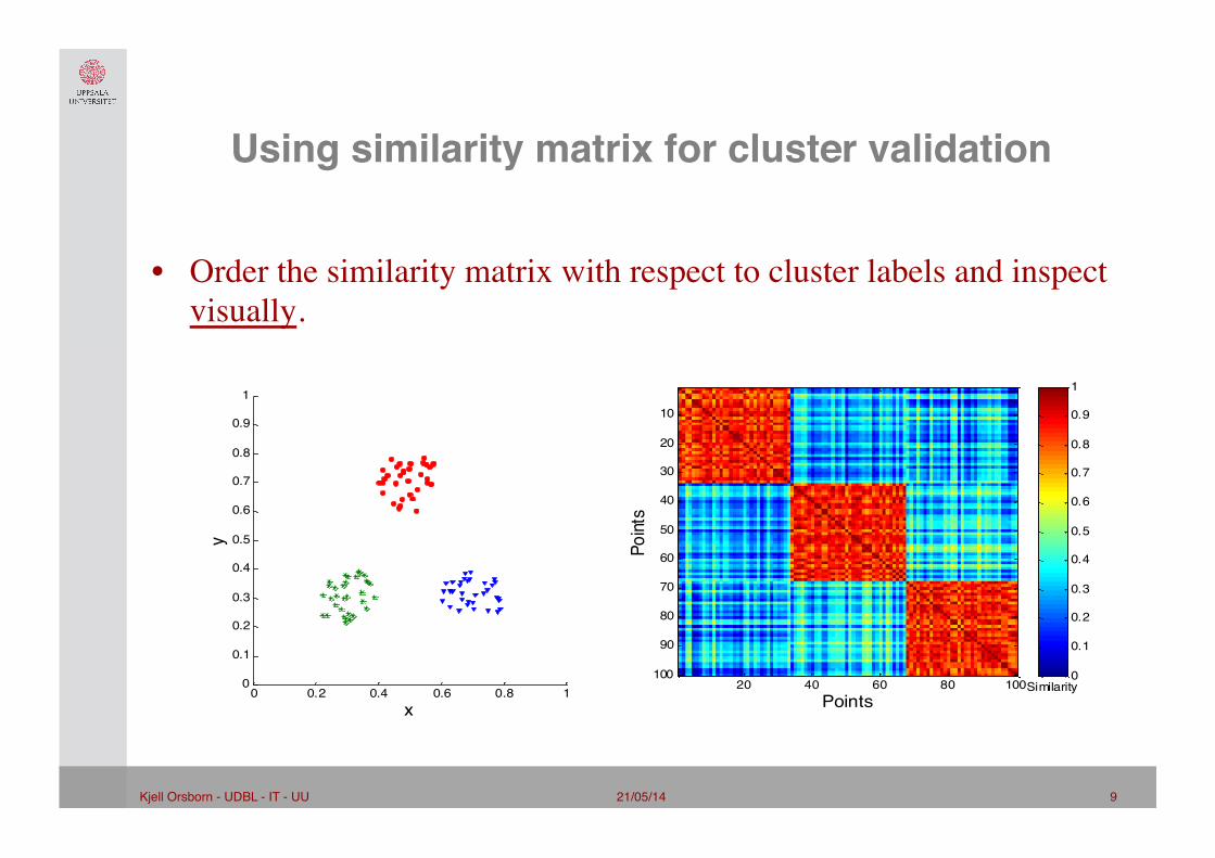
Using similarity matrix for cluster validation"
• Order the similarity matrix with respect to cluster labels and inspect visually.
0 0.2 0.4 0.6 0.8 10
0.1
0.2
0.3
0.4
0.5
0.6
0.7
0.8
0.9
1
x
y
Points
Points
20 40 60 80 100
10
20
30
40
50
60
70
80
90
100Similarity
0
0.1
0.2
0.3
0.4
0.5
0.6
0.7
0.8
0.9
1
21/05/14 10 Kjell Orsborn - UDBL - IT - UU!
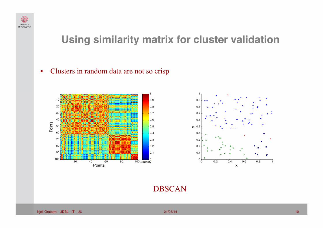
Using similarity matrix for cluster validation"
• Clusters in random data are not so crisp
Points
Points
20 40 60 80 100
10
20
30
40
50
60
70
80
90
100Similarity
0
0.1
0.2
0.3
0.4
0.5
0.6
0.7
0.8
0.9
1
DBSCAN
0 0.2 0.4 0.6 0.8 10
0.1
0.2
0.3
0.4
0.5
0.6
0.7
0.8
0.9
1
x
y

21/05/14 11 Kjell Orsborn - UDBL - IT - UU!
Points
Points
20 40 60 80 100
10
20
30
40
50
60
70
80
90
100Similarity
0
0.1
0.2
0.3
0.4
0.5
0.6
0.7
0.8
0.9
1
Using similarity matrix for cluster validation"
• Clusters in random data are not so crisp
K-means
0 0.2 0.4 0.6 0.8 10
0.1
0.2
0.3
0.4
0.5
0.6
0.7
0.8
0.9
1
x
y

21/05/14 12 Kjell Orsborn - UDBL - IT - UU!
Using similarity matrix for cluster validation"
• Clusters in random data are not so crisp
0 0.2 0.4 0.6 0.8 10
0.1
0.2
0.3
0.4
0.5
0.6
0.7
0.8
0.9
1
x
y
Points
Points
20 40 60 80 100
10
20
30
40
50
60
70
80
90
100Similarity
0
0.1
0.2
0.3
0.4
0.5
0.6
0.7
0.8
0.9
1
Complete Link

21/05/14 13 Kjell Orsborn - UDBL - IT - UU!
Using similarity matrix for cluster validation"
• Clusters of non-globular clusterings are not as clearly separated
1 2
3
5
6
4
7
DBSCAN
0
0.1
0.2
0.3
0.4
0.5
0.6
0.7
0.8
0.9
1
500 1000 1500 2000 2500 3000
500
1000
1500
2000
2500
3000

21/05/14 14 Kjell Orsborn - UDBL - IT - UU!
Internal measures: SSE"• Internal index: Used to measure the goodness of a clustering structure without
respect to external information – SSE
• SSE is good for comparing two clusterings or two clusters (average SSE). • Can also be used to estimate the number of clusters
2 5 10 15 20 25 300
1
2
3
4
5
6
7
8
9
10
K
SSE
5 10 15
-6
-4
-2
0
2
4
6
21/05/14 15 Kjell Orsborn - UDBL - IT - UU!
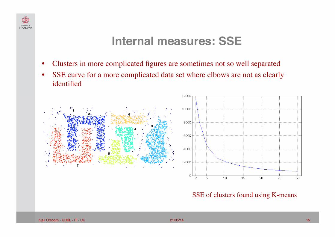
Internal measures: SSE"• Clusters in more complicated figures are sometimes not so well separated • SSE curve for a more complicated data set where elbows are not as clearly
identified
1 2
3
5
6
4
7
SSE of clusters found using K-means

21/05/14 16 Kjell Orsborn - UDBL - IT - UU!
Unsupervised cluster validity measure"
• More generally, given K clusters:���
– Validity(Ci): a function of cohesion, separation, or both – Weight wi associated with each cluster i
– For SSE: • wi = 1 • validity(Ci) = ( )2∑
∈
−iCx
ix µ
21/05/14 17 Kjell Orsborn - UDBL - IT - UU!
• Cluster cohesion: measures how closely related objects are in a cluster
• Cluster separation: measures how distinct or well-separated a cluster is from other clusters
Internal measures: Cohesion and Separation"
21/05/14 18 Kjell Orsborn - UDBL - IT - UU!
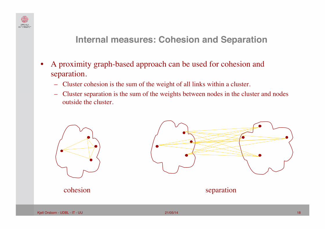
Internal measures: Cohesion and Separation"
• A proximity graph-based approach can be used for cohesion and separation.
– Cluster cohesion is the sum of the weight of all links within a cluster. – Cluster separation is the sum of the weights between nodes in the cluster and nodes
outside the cluster.
cohesion separation

21/05/14 19 Kjell Orsborn - UDBL - IT - UU!
Internal measures: Cohesion and Separation"
• A prototype-based approach can also be used for cohesion and separation. – Cluster cohesion is the sum of the proximities with respect to the prototype (centroid or
mediod) of the cluster. – Cluster separation is measured by the proximity of the cluster prototypes.
cohesion separation

21/05/14 20 Kjell Orsborn - UDBL - IT - UU!
Graph-based versus Prototype-based views"

21/05/14 21 Kjell Orsborn - UDBL - IT - UU!
Graph-based view"
• Cluster cohesion: measures how closely related objects are in a cluster ���������
• Cluster separation: measures how distinct or well-separated a cluster is from other clusters
∑∈∈
=
iiCyCx
i yxproximityCCohesion,
),()(
∑∈∈
=
jiCyCx
ji yxproximityCCSeparation,
),(),(

21/05/14 22 Kjell Orsborn - UDBL - IT - UU!
Prototype-based view"
• Cluster Cohesion: ���������
– Equivalent to SSE if proximity is square of Euclidean distance���
• Cluster Separation:
∑∈
=iCx
ii cxproximityCCohesion ),()(
),()(),(),(
ccproximityCSeparationccproximityCCSeparation
ii
jiji
=
=

21/05/14 23 Kjell Orsborn - UDBL - IT - UU!
Unsupervised cluster validity measures"

21/05/14 24 Kjell Orsborn - UDBL - IT - UU!
Prototype-based vs Graph-based cohesion"
• For SSE and points in Euclidean space, it can be shown that average pairwise difference between points in a cluster is equivalent to SSE of the cluster

21/05/14 25 Kjell Orsborn - UDBL - IT - UU!
Total Sum of Squares (TSS)"
c: overall mean ci: centroid of each cluster Ci
mi: number of points in cluster Ci
c c1 c2
c3
∑
∑∑
∑
=
= ∈
=
=
=
k
iii
k
i Cxi
ccdistmSSB
cxdistSSE
cxdistTSS
i
1
2
1
2
2
),(
),(
),(

21/05/14 26 Kjell Orsborn - UDBL - IT - UU!
Total Sum of Squares (TSS)"
1 2 3 4 5 × × × m1 m2
m
9)35.4(2)5.13(21)5.45()5.44()5.12()5.11(
10)35()34()32()31(
22
2222
2222
=−×+−×=
=−+−+−+−=
=−+−+−+−=
SSBSSETSSK=2 clusters:
0)33(410)35()34()23()13(10)35()34()32()31(
2
2222
2222
=−×=
=−+−+−+−=
=−+−+−+−=
SSBSSETSSK=1 cluster:
TSS = SSE + SSB

21/05/14 27 Kjell Orsborn - UDBL - IT - UU!
Total Sum of Squares (TSS)"
TSS = SSE + SSB
• Given a data set, TSS is fixed
• A clustering with large SSE has small SSB, while one with small SSE has large SSB
• Goal is to minimize SSE and maximize SSB
21/05/14 28 Kjell Orsborn - UDBL - IT - UU!
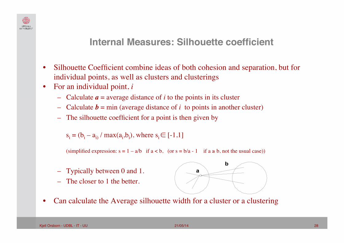
Internal Measures: Silhouette coefficient"
• Silhouette Coefficient combine ideas of both cohesion and separation, but for individual points, as well as clusters and clusterings
• For an individual point, i – Calculate a = average distance of i to the points in its cluster – Calculate b = min (average distance of i to points in another cluster) – The silhouette coefficient for a point is then given by ������si = (bi – ai) / max(ai,bi), where si ∈ [-1,1]������(simplified expression: s = 1 – a/b if a < b, (or s = b/a - 1 if a ≥ b, not the usual case))
– Typically between 0 and 1. – The closer to 1 the better.
• Can calculate the Average silhouette width for a cluster or a clustering
ab
21/05/14 29 Kjell Orsborn - UDBL - IT - UU!
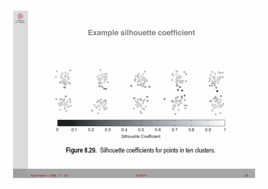
Example silhouette coefficient"
21/05/14 30 Kjell Orsborn - UDBL - IT - UU!
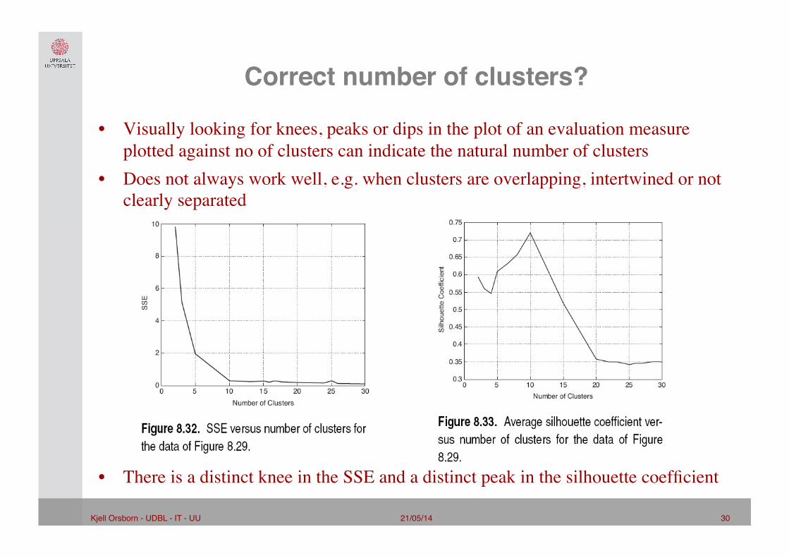
Correct number of clusters?"
• Visually looking for knees, peaks or dips in the plot of an evaluation measure plotted against no of clusters can indicate the natural number of clusters
• Does not always work well, e.g. when clusters are overlapping, intertwined or not clearly separated���������������������������������
• There is a distinct knee in the SSE and a distinct peak in the silhouette coefficient

21/05/14 31 Kjell Orsborn - UDBL - IT - UU!
Clustering tendency"
• Methods to evaluation if data has clusters without clustering���
• Most common approach in Euclidian space is to apply statistical test for spatial randomness – can be quite challenging to select correct model and parameters ���
• Example of Hopkins statistic (se blackboard example)

21/05/14 32 Kjell Orsborn - UDBL - IT - UU!
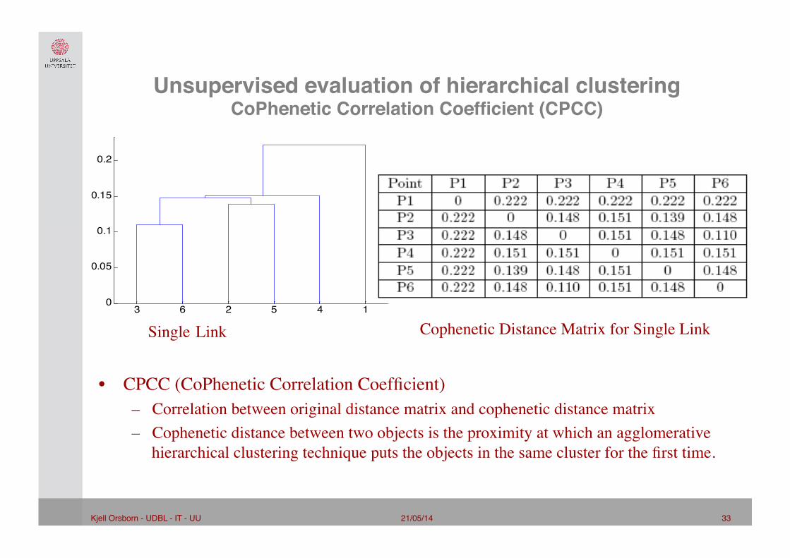
Unsupervised evaluation of hierarchical clusteringCoPhenetic Correlation Coefficient (CPCC)"
Distance matrix:
Single Link
3 6 2 5 4 10
0.05
0.1
0.15
0.2
21/05/14 33 Kjell Orsborn - UDBL - IT - UU!
Unsupervised evaluation of hierarchical clusteringCoPhenetic Correlation Coefficient (CPCC)"
• CPCC (CoPhenetic Correlation Coefficient) – Correlation between original distance matrix and cophenetic distance matrix – Cophenetic distance between two objects is the proximity at which an agglomerative
hierarchical clustering technique puts the objects in the same cluster for the first time.
3 6 2 5 4 10
0.05
0.1
0.15
0.2
Cophenetic Distance Matrix for Single Link Single Link

21/05/14 34 Kjell Orsborn - UDBL - IT - UU!
Unsupervised evaluation of hierarchical clusteringCoPhenetic Correlation Coefficient (CPCC)"
3 6 2 5 4 10
0.05
0.1
0.15
0.2
3 6 4 1 2 50
0.05
0.1
0.15
0.2
0.25
0.3
0.35
0.4
Single Link
Complete Link
21/05/14 35 Kjell Orsborn - UDBL - IT - UU!
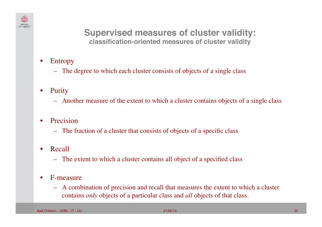
Supervised measures of cluster validity:classification-oriented measures of cluster validity"
• Entropy – The degree to which each cluster consists of objects of a single class
• Purity – Another measure of the extent to which a cluster contains objects of a single class
• Precision – The fraction of a cluster that consists of objects of a specific class ���
• Recall – The extent to which a cluster contains all object of a specified class ���
• F-measure – A combination of precision and recall that measures the extent to which a cluster
contains only objects of a particular class and all objects of that class.

21/05/14 36 Kjell Orsborn - UDBL - IT - UU!
External measures of cluster validity: Entropy and Purity"

21/05/14 37 Kjell Orsborn - UDBL - IT - UU!
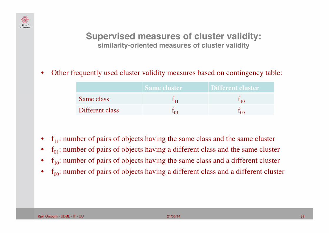
Supervised measures of cluster validity:similarity-oriented measures of cluster validity"
• A similarity-oriented measure of cluster validity is based on the idea that any two objects in the same cluster should be in the same class.���
• Can be expressed as comparing the two matrices: – Ideal cluster similarity matrix that has a 1 in the ijth entry if two objects i and j are in the
same cluster and 0 otherwise. – Ideal class similarity matrix defined with respect to class labels which has a 1 in the ijth
entry if two objects i and j belong to the same class and 0 otherwise.
• The correlation between these two matrices, called the Γ (gamma) statistic, can be taken as a measure of cluster validity

21/05/14 38 Kjell Orsborn - UDBL - IT - UU!
Supervised measures of cluster validity:similarity-oriented measures of cluster validity"
• Correlation between cluster and class matrices – Five data points: p1, p2, p3, p4 and p5. – Two clusters: C1 = {p1, p2, p3} and C2 = {p4, p5} – Two classes: L1 = {p1, p2} and L2 = {p3, p4, p5} – Correlation between these matrices is 0,359 (?).
21/05/14 39 Kjell Orsborn - UDBL - IT - UU!
Supervised measures of cluster validity:similarity-oriented measures of cluster validity"
• Other frequently used cluster validity measures based on contingency table:
• f11: number of pairs of objects having the same class and the same cluster • f01: number of pairs of objects having a different class and the same cluster • f10: number of pairs of objects having the same class and a different cluster • f00: number of pairs of objects having a different class and a different cluster
Same cluster Different cluster Same class f11 f10
Different class f01 f00

21/05/14 40 Kjell Orsborn - UDBL - IT - UU!
Supervised measures of cluster validity:similarity-oriented measures of cluster validity"
• Other frequently used cluster validity measures based on contingency table:
• Example of Rand statistics and Jaccard coefficient (on blackboard)
Same cluster Different cluster Same class f11 = 2 f10 = 2 Different class f01 = 2 f00 = 4

21/05/14 41 Kjell Orsborn - UDBL - IT - UU!
Supervised measures of cluster validity:cluster validity for hierarchical clustering's"
• Supervised evaluation of hierarchical clustering is more difficult – E.g. preexisting hierarchical structure might be hard to find
• Evaluation of hierarchical clustering with respect to a flat set of class labels • Idea is to evaluate whether the hierarchical clustering, for each class, contains at
least one cluster that is relatively pure and contain most objects of that class. • Compute (for each class) the F-measure for each cluster in the hierarchy. • Retrieve the maximum F-measure for each class attained for any cluster • Calculate the total F-measure as the weighted average of all per-class F-measures
• F = sum(j) mj/m max(i) F(i,j)

21/05/14 42 Kjell Orsborn - UDBL - IT - UU!
Supervised measures of cluster validity:cluster validity for hierarchical clustering's"
● Hierarchical F-measure:

21/05/14 43 Kjell Orsborn - UDBL - IT - UU!
Significance of cluster validity measures?"
• How to interpret the significance of a calculated evaluation measure?
• Min/max values gives some guidance���
• However min/max might not be available or scale may affect interpretation���
• Different application might tolerate different values ���
• Common solution: to interpret value of validity measure in statistical terms.
– See following examples:

21/05/14 44 Kjell Orsborn - UDBL - IT - UU!
Framework for cluster validity"
• Need a framework to interpret any measure. – For example, if our measure of evaluation has the value, 10, is that good, fair, or
poor?
• Statistics provide a framework for cluster validity – The more “atypical” a clustering result is, the more likely it represents valid structure
in the data – Can compare the values of an index that result from random data or clusterings to
those of a clustering result. • If the value of the index is unlikely, then the cluster results are valid
• For comparing the results of two different sets of cluster analyses, a framework is less necessary.
– However, there is the question of whether the difference between two index values is significant
21/05/14 45 Kjell Orsborn - UDBL - IT - UU!
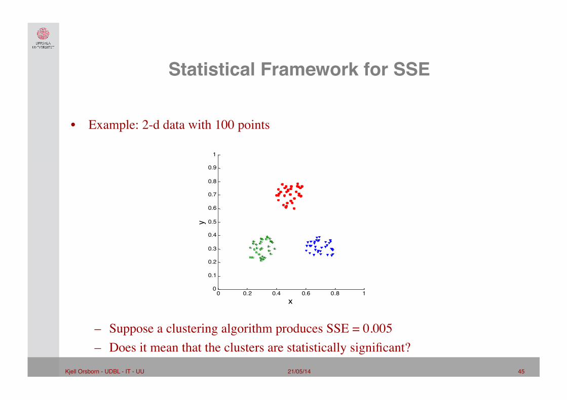
Statistical Framework for SSE"
• Example: 2-d data with 100 points
– Suppose a clustering algorithm produces SSE = 0.005 – Does it mean that the clusters are statistically significant?
0 0.2 0.4 0.6 0.8 10
0.1
0.2
0.3
0.4
0.5
0.6
0.7
0.8
0.9
1
x
y

21/05/14 46 Kjell Orsborn - UDBL - IT - UU!
Statistical framework for SSE"• Example continued:
– Generate 500 sets of random data points of size 100 distributed over the range 0.2 – 0.8 for x and y values
– Perform clustering with k = 3 clusters for each data set – Plot histogram of SSE and compare with the value 0.005 for the 3 well-separated
clusters
0.016 0.018 0.02 0.022 0.024 0.026 0.028 0.03 0.032 0.0340
5
10
15
20
25
30
35
40
45
50
SSE
Count
0 0.2 0.4 0.6 0.8 10
0.1
0.2
0.3
0.4
0.5
0.6
0.7
0.8
0.9
1
x
y

21/05/14 47 Kjell Orsborn - UDBL - IT - UU!
Statistical framework for correlation"
• Correlation of incidence and proximity matrices for the K-means clusterings of the following two data sets.
0 0.2 0.4 0.6 0.8 10
0.1
0.2
0.3
0.4
0.5
0.6
0.7
0.8
0.9
1
x
y
0 0.2 0.4 0.6 0.8 10
0.1
0.2
0.3
0.4
0.5
0.6
0.7
0.8
0.9
1
x
y
Corr = -0.9235���(statistically significant)
Corr = -0.5810���(not statistically
significant)

21/05/14 48 Kjell Orsborn - UDBL - IT - UU!
Final comment on cluster validity"
“The validation of clustering structures is the most difficult and frustrating part of cluster analysis.
Without a strong effort in this direction, cluster analysis will remain a black art accessible only to those true believers who have experience and great courage.”
Algorithms for Clustering Data, Jain and Dubes
21/05/14 49 Tore Risch- UDBL - IT - UU!
Alt. Clustering Techniques Cluster analysis: additional issues and algorithms
(Tan, Steinbach, Kumar ch. 9)"
Kjell Orsborn ���
Department of Information Technology Uppsala University, Uppsala, Sweden

21/05/14 50 Kjell Orsborn - UDBL - IT - UU!
Characteristics of data, clusters and clustering algorithms"
• No algorithm suitable for all types of data, clusters, and applications
• Characteristics of data, clusters, and algorithms strongly impact clustering
• Important for understanding, describing and comparing clustering techniques.

21/05/14 51 Kjell Orsborn - UDBL - IT - UU!
Characteristics of data"• High dimensionality
– Problem with density and proximity measures – Dimensionality reduction techniques one approach to address this problem – Redefinition of proximity and density is another
• Size – Many algorithms have time or space complexity of O(m2), m being the no of objects
• Sparseness – What type of sparse data? Asymmetric attributes? Magnitude important or just occurences?
• Noise and outliers – How are noise and outliers affecting a specific algorithm? (dealt with in Chameleon, SNN density,
CURE) • Types of attributes and data set
– Different proximity and density measures needed for different types of data • Scale
– Normalization can be required • Mathematical properties of the data space
– E.g. is mean or density meaningful for your data?

21/05/14 52 Kjell Orsborn - UDBL - IT - UU!
Characteristics of clusters "• Data distribution
– Some clustering algorithms assume a particular type of distribution of data, e.g. mixture models
• Shape – Can a specific algorithm handle the expected cluster shapes? (DBSCAN, Chameleon,
CURE) • Differing sizes
– Can a specific algorithm handle varying cluster sizes? • Differing densities
– Can a specific algorithm handle varying cluster densities? (SNN density) • Poorly separated clusters
– Can a specific algorithm handle overlapping clusters? • Relationships among clusters
– E.g. self-organizing maps (SOM) considers the relationships between clusters • Subspace clusters
– Clusters can exist in many distinct subspaces (DENCLUE)

21/05/14 53 Kjell Orsborn - UDBL - IT - UU!
Characteristics of clustering algorithms "
• Order dependence – Quality and number of clusters can be order dependent, e.g. SOM
• Nondeterminism – E.g. K-means produces different results for every execution
• Scalability – Required for large data sets
• Parameter selection – Can be challenging to set parameter values
• Transforming the clustering problem to another domain – E.g. graph partitioning
• Treating clustering as an optimization problem – In reality one need some heuristics that produce good (but maybe not optimal) results
21/05/14 54 Kjell Orsborn - UDBL - IT - UU!
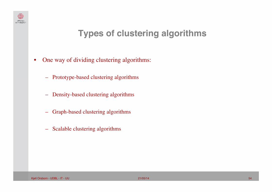
Types of clustering algorithms "
• One way of dividing clustering algorithms:
– Prototype-based clustering algorithms
– Density-based clustering algorithms
– Graph-based clustering algorithms
– Scalable clustering algorithms

21/05/14 55 Kjell Orsborn - UDBL - IT - UU!
Prototype-based clustering algorithms"
• K-means – centroid-based
• Fuzzy clustering – Objects are allowed to belong to more than one cluster – Relies on fuzzy set theory that allows an object to belong to a set with a degree of
membership between 0 and 1. – Fuzzy c-means
• Mixture models clustering – Clusters modeled as statistical distributions – EM (expectation-maximization) algorithm
• Self-organizing maps (SOM) – Clusters constrained to have fixed relationships to neighbours

21/05/14 56 Kjell Orsborn - UDBL - IT - UU!
Example of Fuzzy c-means clustering"

21/05/14 57 Kjell Orsborn - UDBL - IT - UU!
Fuzzy c-means clustering pros and cons"
• Do not restrict data points to belong to one cluster – instead indicate the degree that a point belong to any cluster
• Also share some strength and weaknesses (like non-globular shapes) of K-means but more computationally intensive

21/05/14 58 Kjell Orsborn - UDBL - IT - UU!
Mixture models clustering"• Clusters modeled as statistical distributions
– Exemplified by EM (expectation-maximization) algorithm

21/05/14 59 Kjell Orsborn - UDBL - IT - UU!
EM (expectation-maximization) algorithm"

21/05/14 60 Kjell Orsborn - UDBL - IT - UU!
EM clustering example"
21/05/14 61 Kjell Orsborn - UDBL - IT - UU!
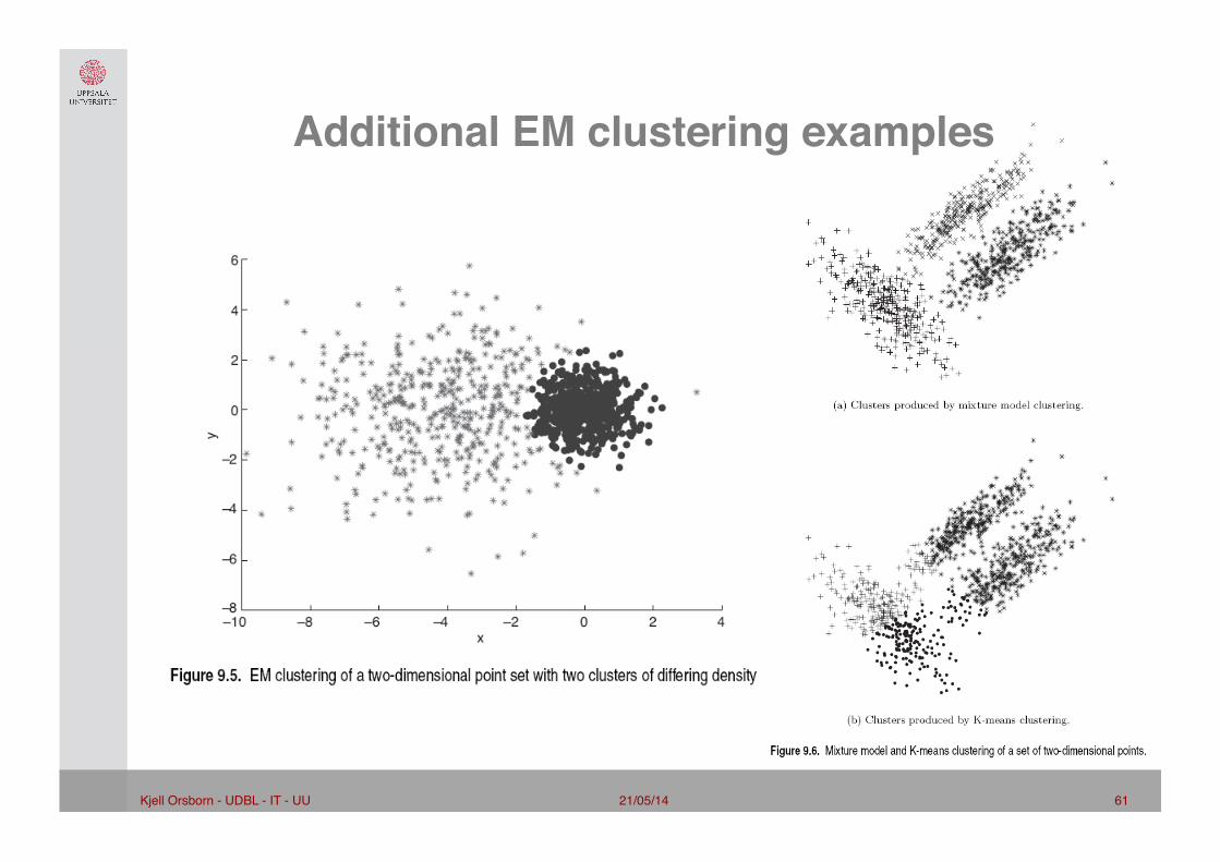
Additional EM clustering examples"

21/05/14 62 Kjell Orsborn - UDBL - IT - UU!
EM clustering pros and cons"
• Can be slow for models including a large number of components or if there are a low number of data points
• Problems of estimating the number of clusters or more generally to chose the exact form of the model
• Noise and outliers might cause problems ���
• More general than K-means using various types of distributions – Can find clusters of different sizes and elliptical shapes
• Condensed description of clusters through a small no of parameters

21/05/14 63 Kjell Orsborn - UDBL - IT - UU!
Self organizing maps (SOM)"• The goal of SOM is to find a set of centroids (reference vectors using SOM terminology)
and assigning each data point to the centroid that provides the best approximation of that data point.
• In self-organizing maps (SOM), centroids have a predetermined topographic ordering relationship
• During the training process, SOM uses each data point to update the closest centroid and nearby centroids in the topographic ordering
• For example, the centroids of a two-dimensional SOM can be viewed as a structure on a 2D-surface that tries to fit the n-dimensional data as good as possible

21/05/14 64 Kjell Orsborn - UDBL - IT - UU!
Example of SOM application"• In self-organizing maps, clusters are constrained to have fixed relationships to
neighbours

21/05/14 65 Kjell Orsborn - UDBL - IT - UU!
Illustration of a self organizing map (SOM)"• Illustration of SOM network where black dots are data and green dots represent
SOM nodes (source: http://www.peltarion.com/).

21/05/14 66 Kjell Orsborn - UDBL - IT - UU!
Self organizing maps pros and cons"
• Related clusters are close which facilitate the interpretation and visualization of clustering results
• Settings of several parameters, neighborhood function, grid type, no of centroids • SOM cluster might not correspond to single natural cluster, it can encompass
several natural clusters or a single natural cluster might span several centroids • Lacks an objective function that can make it problematic to compare different
SOM clustering results • Convergence can be slow and is not guaranteed but normally fulfilled
21/05/14 67 Kjell Orsborn - UDBL - IT - UU!
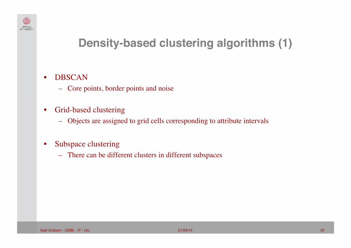
Density-based clustering algorithms (1)"
• DBSCAN – Core points, border points and noise
• Grid-based clustering – Objects are assigned to grid cells corresponding to attribute intervals
• Subspace clustering – There can be different clusters in different subspaces

21/05/14 68 Kjell Orsborn - UDBL - IT - UU!
Density-based clustering algorithms (2)"• Grid-based clustering:

21/05/14 69 Kjell Orsborn - UDBL - IT - UU!
Grid-based clustering pros and cons"
• Grid-based clustering can be very efficient and effective with a O(m), m no of points, complexity for defining the grid and an overall complexity of O(m log m)
• Dependent of the choice of density threshold – To high – clusters will be lost – To low – separate clusters may be joined. – Differing densities might make it hard to find a single threshold that works for complete
data space • Rectangular grid may have problems accurately capturing circular boundaries • Grid-based clustering tends to work poorly for high-dimensional data
21/05/14 70 Kjell Orsborn - UDBL - IT - UU!
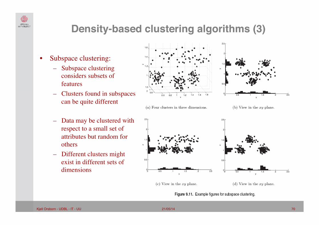
Density-based clustering algorithms (3)"
• Subspace clustering: – Subspace clustering
considers subsets of features
– Clusters found in subspaces can be quite different
– Data may be clustered with respect to a small set of attributes but random for others
– Different clusters might exist in different sets of dimensions

21/05/14 71 Kjell Orsborn - UDBL - IT - UU!
Density-based clustering algorithms (4)"• CLIQUE (clustering in quest)
– Grid-based clustering that methodologically finds subspace clusters – No of subspaces is exponential in no of dimensions so some efficient pruning technique
needed – CLIQUE relies on the monotonicity property of density-based clusters: if a set of points
forms a density-based cluster in k-dimensions, then the same point is also part of a density-based cluster in all possible subsets of those dimensions.
– Based on well-known Apriori principle from association analysis

21/05/14 72 Kjell Orsborn - UDBL - IT - UU!
Density-based clustering algorithms (5)"
• CLIQUE pros and cons – Well understood since based on well-known Apriori principle – Can summarize the list of cells in clusters with a small set of inequalities
– Clusters can overlap and make interpretation difficult – Potential exponential time complexity – to many cells might be generated for
lower values of k, i.e. for low dimensions.

21/05/14 73 Kjell Orsborn - UDBL - IT - UU!
Density-based clustering algorithms (6)"• DENCLUE (density clustering)
– Models the overall density of a set of points as the sum of the influence (or kernel) functions associated with each point
– Based on kernel density estimation, a well-developed area of statistics. – Peaks (local density attractors) forms the basis for forming clusters – A minimum density threshold, ξ, separates clusters from data points considered to be
noise
– Grid-based implementation defines neighborhood and reduces complexity

21/05/14 74 Kjell Orsborn - UDBL - IT - UU!
Density-based clustering algorithms (7)"• DENCLUE:

21/05/14 75 Kjell Orsborn - UDBL - IT - UU!
Density-based clustering algorithms (8)"
• DENCLUE pros and cons – Solid theoretical foundation – Good at handling noise and outliers and finding clusters of different shapes and
sizes
– Can be computationally expensive – Susceptible to accuracy dependence to choice of grid size – Problems with high-dimensionality and different densities

21/05/14 76 Kjell Orsborn - UDBL - IT - UU!
Graph-based clustering algorithms (1)"• In graph-based clustering data objects are represented as nodes and proximity as the edge
weight between two corresponding nodes. – Discussed agglomerative (hierarchical) clustering algorithms in dm1 course.���
• Here some more advanced graph-based clustering algorithms are presented that applies different subsets of the following key approaches:
• Sparsification of proximity graph keeping only connections of an object to its nearest neighbours
– Useful for handling noise and outliers – Makes it possible to apply efficient graph partitioning algorithms
• Similarity measures between objects based on the no of shared nearest neighbours – Useful for handling problems with high dimensionality and varying density
• Define core points as a basis for cluster generation – Requires density-based concept for (sparsified) proximity graphs – Useful for handling differing shapes and sizes
• Use information in proximity graph for more sophisticated merging strategies – E.g. will merged cluster have similar characteristics as original unmerged clusters

21/05/14 77 Kjell Orsborn - UDBL - IT - UU!
Graph-based clustering algorithms (2)"
• Graph-Based clustering uses the proximity graph – Start with the proximity matrix – Consider each point as a node in a graph – Each edge between two nodes has a weight which is the proximity between the two
points – Initially the proximity graph is fully connected – MIN (single-link) and MAX (complete-link) can be viewed as starting with this graph
• In the simplest case, clusters are connected components in the graph.
21/05/14 78 Kjell Orsborn - UDBL - IT - UU!
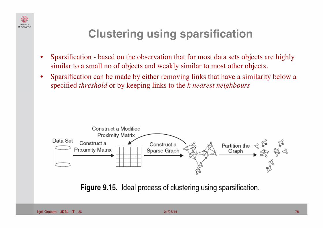
Clustering using sparsification"
• Sparsification - based on the observation that for most data sets objects are highly similar to a small no of objects and weakly similar to most other objects.
• Sparsification can be made by either removing links that have a similarity below a specified threshold or by keeping links to the k nearest neighbours

21/05/14 79 Kjell Orsborn - UDBL - IT - UU!
Clustering using sparsification …"
• The amount of data that needs to be processed is drastically reduced – Sparsification can eliminate more than 99% of the entries in a proximity matrix – The amount of time required to cluster the data is drastically reduced – The size of the problems that can be handled is increased���
• Clustering may work better – Sparsification techniques keep the connections to the most similar (nearest) neighbors of
a point while breaking the connections to less similar points. – The nearest neighbors of a point tend to belong to the same class as the point itself. – This reduces the impact of noise and outliers and sharpens the distinction between
clusters. ���
• Sparsification facilitates the use of graph partitioning algorithms – The Chameleon and hypergraph-based clustering
21/05/14 80 Kjell Orsborn - UDBL - IT - UU!
Graph-based clustering algorithms (3)"
• MST (minimum spanning tree) clustering and OPPOSSUM (optimal partitioning of sparse similarities using Metis)
– Both MST and OPPOSSUM relies solely on sparsification – Oppossum uses the METIS graph partitioning algorithm – MST is equivalent to single-link clustering and was treated in dm1 – Oppossum:
• 1) compute a sparsified similarity graph • 2) partition the graph into k clusters using METIS
• Pros and cons – OPPOSSUM is simple and fast – Roughly equal-sized clusters can be good or bad – equal-sized clusters means clusters can be broken or combined

21/05/14 81 Kjell Orsborn - UDBL - IT - UU!
Graph-based clustering algorithms (4)"
• Chameleon – Hierarchical clustering with dynamic modeling – Combines an initial partitioning of data and a novel hierarchical clustering scheme – Use sparsification and self similarity
• Jarvis-Patrick and ROCK – Shared-nearest neighbour (SNN) similarity
• SNN density-based clustering algorithm – Applies shared-nearest neighbour density

21/05/14 82 Kjell Orsborn - UDBL - IT - UU!
Limitations of Current Cluster Merging Schemes"
• Existing cluster merging schemes in hierarchical clustering algorithms are static in nature���
– MIN or CURE: • merge two clusters based on their closeness (or minimum distance)
– GROUP-AVERAGE: • merge two clusters based on their average connectivity

21/05/14 83 Kjell Orsborn - UDBL - IT - UU!
Limitations of Current Cluster Merging Schemes"
Closeness schemes will merge (a) and (b)
(a) (b)
(c)
(d)
Average connectivity schemes will merge (c) and (d)

21/05/14 84 Kjell Orsborn - UDBL - IT - UU!
Chameleon: Clustering Using Dynamic Modeling"
• Adapt to the characteristics of the data set to find the natural clusters • Use a dynamic model to measure the similarity between clusters
– Main property is the relative closeness and relative inter-connectivity of the cluster
– Two clusters are combined if the resulting cluster shares certain properties with the constituent clusters
– The merging scheme preserves self-similarity
• One of the areas of application is spatial data

21/05/14 85 Kjell Orsborn - UDBL - IT - UU!
Characteristics of spatial data sets"
• Clusters are defined as densely populated regions of the space
• Clusters have arbitrary shapes, orientation, and non-uniform sizes ���
• Difference in densities across clusters and variation in density within clusters ���
• Existence of special artifacts (streaks) and noise
The clustering algorithm must address the above characteristics and also require
minimal supervision.

21/05/14 86 Kjell Orsborn - UDBL - IT - UU!
Chameleon: steps"
• Preprocessing Step:��� ���Represent the data by a graph
– Given a set of points, construct the k-nearest-neighbor (k-NN) graph to capture the relationship between a point and its k nearest neighbors
– Concept of neighborhood is captured dynamically (even if region is sparse)
• Phase 1: ������Use a multilevel graph partitioning algorithm on the graph to find a large number of clusters of well-connected vertices
– Each cluster should contain mostly points from one “true” cluster, i.e., is a sub-cluster of a “real” cluster

21/05/14 87 Kjell Orsborn - UDBL - IT - UU!
Chameleon: steps … "
• Phase 2: ������Use Hierarchical Agglomerative Clustering to merge sub-clusters
– Two clusters are combined if the resulting cluster shares certain properties with the constituent clusters
– Two key properties used to model cluster similarity: • Relative Interconnectivity: Absolute interconnectivity of two clusters normalized by the
internal connectivity of the clusters
• Relative Closeness: Absolute closeness of two clusters normalized by the internal closeness of the clusters

21/05/14 88 Kjell Orsborn - UDBL - IT - UU!
Chameleon pros and cons "
• Clusters spatial data effectively even when data include noise and outliers • Handles clusters of different shapes sizes and density
• Assumes groups of data from sparsification are belong to the same true cluster and cannot separate objects through the agglomerative hierarchical clustering step
– i.e. Chameleon can have problems in high-dimensional space where partitioning will not produce subclusters

21/05/14 89 Kjell Orsborn - UDBL - IT - UU!
Experimental Results: CHAMELEON"

21/05/14 90 Kjell Orsborn - UDBL - IT - UU!
Experimental Results: CHAMELEON"

21/05/14 91 Kjell Orsborn - UDBL - IT - UU!
Experimental Results: CHAMELEON"
21/05/14 92 Kjell Orsborn - UDBL - IT - UU!
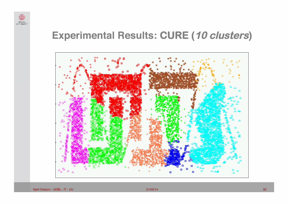
Experimental Results: CURE (10 clusters)"

21/05/14 93 Kjell Orsborn - UDBL - IT - UU!
Experimental Results: CURE (15 clusters)"

21/05/14 94 Kjell Orsborn - UDBL - IT - UU!
Experimental Results: CHAMELEON

21/05/14 95 Kjell Orsborn - UDBL - IT - UU!
Experimental Results: CURE (9 clusters)"

21/05/14 96 Kjell Orsborn - UDBL - IT - UU!
Experimental Results: CURE (15 clusters)"

21/05/14 97 Kjell Orsborn - UDBL - IT - UU!
i j i j 4
Shared Nearest Neighbour (SNN) Approach"
• SNN graph: the weight of an edge is the number of shared neighbours between vertices given that the vertices are connected

21/05/14 98 Kjell Orsborn - UDBL - IT - UU!
Creating the SNN Graph"
Sparse Graph
Link weights are similarities between neighboring points
Shared Near Neighbor Graph
Link weights are number of Shared Nearest Neighbors

21/05/14 99 Kjell Orsborn - UDBL - IT - UU!
Jarvis-Patrick Clustering"
• First, the k-nearest neighbors of all points are found – In graph terms this can be regarded as breaking all but the k strongest links from a point
to other points in the proximity graph
• A pair of points is put in the same cluster if – any two points share more than T neighbors and – the two points are in each others k nearest neighbor list
• For instance, we might choose a nearest neighbor list of size 20 and put points in the same cluster if they share more than 10 near neighbors
• Jarvis-Patrick clustering is too brittle

21/05/14 100 Kjell Orsborn - UDBL - IT - UU!
Jarvis-Patrick clustering pros and cons"
• SNN similarity means JP is good at handling noise and outliers • Can handle clusters of different sizes, shapes and densities • Works well in high-dimensional space, especially finding tight clusters of strongly
related objects
• Jarvis-Patrick clustering is somewhat brittle since split/join may depend on very few links
• May not cluster all objects - but that can be handled separately • Complexity O(m2) (or O(m log m) in low-dimensional space) • Finding best parameter settings can be challenging

21/05/14 101 Kjell Orsborn - UDBL - IT - UU!
When Jarvis-Patrick Works Reasonably Well"
Original Points Jarvis Patrick Clustering
6 shared neighbors out of 20

21/05/14 102 Kjell Orsborn - UDBL - IT - UU!
Smallest threshold, T, that does not merge clusters.
Threshold of T - 1
When Jarvis-Patrick does NOT work well"
21/05/14 103 Kjell Orsborn - UDBL - IT - UU!
ROCK (RObust Clustering using linKs)"
• ROCK uses a similar “number of shared neighbors” proximity measure as Jarvis-Patrick.
• Clustering algorithm for data with categorical and Boolean attributes – A pair of points is defined to be neighbors if their similarity is greater than some
threshold – Use a hierarchical clustering scheme to cluster the data. ���
1. Obtain a sample of points from the data set 2. Compute the link value for each set of points, i.e., transform the original
similarities (computed by Jaccard coefficient) into similarities that reflect the number of shared neighbors between points
3. Perform an agglomerative hierarchical clustering on the data using the “number of shared neighbors” as similarity measure and maximizing “the shared neighbors” objective function
4. Assign the remaining points to the clusters that have been found

21/05/14 104 Kjell Orsborn - UDBL - IT - UU!
SNN Density Clustering"
• The Shared Nearest Neighbour Density algorithm is based upon SNN similarity in combination with a DBSCAN approach���
• SNN density measures the degree to which a point is surrounded by similar points ���
• High/low density areas tend to have high SNN density���
• Transition areas (high-low density) tend to have low SNN density

21/05/14 105 Kjell Orsborn - UDBL - IT - UU!
SNN Density"
a) All Points b) High SNN Density
c) Medium SNN Density d) Low SNN Density
21/05/14 106 Kjell Orsborn - UDBL - IT - UU!
SNN Density clustering algorithm"
1. Compute the similarity matrix���This corresponds to a similarity graph with data points for nodes and edges whose weights are the similarities between data points
2. Sparsify the similarity matrix by keeping only the k most similar neighbors ���This corresponds to only keeping the k strongest links of the similarity graph
3. Construct the shared nearest neighbor graph from the sparsified similarity matrix. ���At this point, we could apply a similarity threshold and find the connected components to obtain the clusters (Jarvis-Patrick algorithm)
4. Find the SNN density of each Point.���Using a user specified parameters, Eps, find the number points that have an SNN similarity of Eps or greater to each point. This is the SNN density of the point

21/05/14 107 Kjell Orsborn - UDBL - IT - UU!
SNN Density clustering algorithm …"
5. Find the core points ���Using a user specified parameter, MinPts, find the core points, i.e., all points that have an SNN density greater than MinPts
6. Form clusters from the core points ���If two core points are within a radius, Eps, of each other they are place in the same cluster
7. Discard all noise points ���All non-core points that are not within a radius of Eps of a core point are discarded
8. Assign all non-noise, non-core points to clusters ���This can be done by assigning such points to the nearest core point
���(Note that steps 4-8 are DBSCAN)
21/05/14 108 Kjell Orsborn - UDBL - IT - UU!
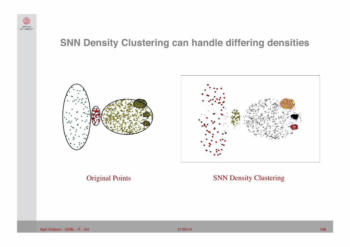
SNN Density Clustering can handle differing densities"
Original Points SNN Density Clustering

21/05/14 109 Kjell Orsborn - UDBL - IT - UU!
SNN Density Clustering can handle other difficult situations"

21/05/14 110 Kjell Orsborn - UDBL - IT - UU!
Finding Clusters of Time Series In Spatio-Temporal Data"
26 SLP Clusters via Shared Nearest Neighbor Clustering (100 NN, 1982-1994)
longitude
latitu
de
-180 -150 -120 -90 -60 -30 0 30 60 90 120 150 180
90
60
30
0
-30
-60
-90
13 26
24 25
22
14
16 20 17 18
19
15
23
1 9
6 4
7 10 12 11
3 5 2
8
21
SNN Clusters of SLP.
SNN Density of SLP Time Series Data
longitude
latitu
de
-180 -150 -120 -90 -60 -30 0 30 60 90 120 150 180
90
60
30
0
-30
-60
-90
SNN Density of Points on the Globe.

21/05/14 111 Kjell Orsborn - UDBL - IT - UU!
Features and limitations of SNN Clustering"
• Has similar strengths and limitations as Jarvis-Patrick clustering
• Does not cluster all the points
• Complexity of SNN Clustering is high – O( n * time to find numbers of neighbours within Eps) – In worst case, this is O(n2) – For lower dimensions, there are more efficient ways to find the nearest
neighbours, such as R* trees and K-D trees • The approach of using core points and SNN density adds power and flexibility

21/05/14 112 Kjell Orsborn - UDBL - IT - UU!
Scalable clustering algorithms"• Issues:
– Storage requirements – Computational requirements
• Approaches: – Multi-dimensional or spatial access methods
• e.g. k-d tree and R*-tree forms hierarchical partition of data space • Also grid-based clustering partition data space
– Bounds on proximities • Reduces no of proximity calculations
– Sampling • Clusters samples of points • E.g. CURE
– Partitioning data objects • Bisecting K-means, CURE
– Summarization • Represents summarizations of data • BIRCH

21/05/14 113 Kjell Orsborn - UDBL - IT - UU!
Scalable clustering algorithms"• Approaches continued:
– Parallel and distributed computation • Parallel and distributed versions of clustering algorithms • Conventional parallel master-slave programming approaches • Map-reduce / hadoop based approaches
• Algorithms specifically design for large-scale clustering – BIRCH (balanced iterative reducing and clustering using hierarchies)
• Builds a compressed tree structure of clustering features (CF) in a CF-tree including measures for inter/intra cluster cohesion and separation
– CURE (clustering using representatives) – CLARANS (clustering large applications based on randomized search)
• Parallel and distributed versions of earlier clustering algorithms – PBIRCH – parallel version of BIRCH – ICLARANS – parallel version of BIRCH – PKMeans (parallel version of k-means), K-Means++ (map reduce versions of K-means) – DBSCAN, Parallel DBSCAN (parallel version of dbscan) , MR-DBSCAN (map reduce versions)

21/05/14 114 Kjell Orsborn - UDBL - IT - UU!
Outline of the BIRCH algorithm"
21/05/14 115 Kjell Orsborn - UDBL - IT - UU!
Hierarchical clustering: revisited"
• Creates nested clusters
• Agglomerative clustering algorithms vary in terms of how the proximity of two clusters are computed
• MIN (single link): susceptible to noise/outliers • MAX/GROUP AVERAGE: ���
may not work well with non-globular clusters
– CURE algorithm tries to handle both problems
• Often starts with a proximity matrix – A type of graph-based algorithm

21/05/14 116 Kjell Orsborn - UDBL - IT - UU!
CURE: another hierarchical approach"• Uses a number of points to represent a cluster���
• Representative points are found by selecting a constant number of points from a cluster and then “shrinking” them toward the center of the cluster
• Cluster similarity is the similarity of the closest pair of representative points from different clusters
• Shrinking representative points toward the center helps avoid problems with noise and outliers
• CURE is better able to handle clusters of arbitrary shapes and sizes
× ×

21/05/14 117 Kjell Orsborn - UDBL - IT - UU!
Outline of the CURE algorithm"
21/05/14 118 Kjell Orsborn - UDBL - IT - UU!
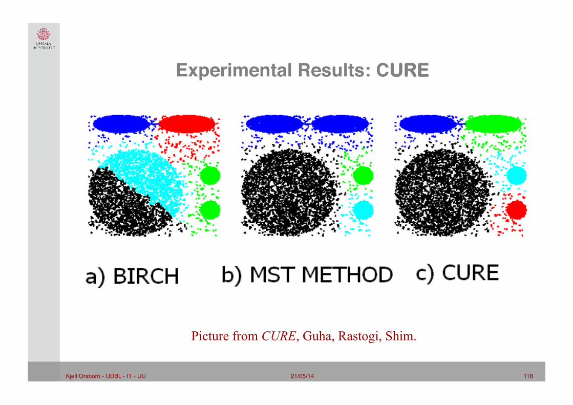
Experimental Results: CURE"
Picture from CURE, Guha, Rastogi, Shim.
21/05/14 119 Kjell Orsborn - UDBL - IT - UU!
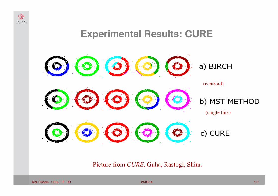
Experimental Results: CURE"
Picture from CURE, Guha, Rastogi, Shim.
(centroid)
(single link)

21/05/14 120 Kjell Orsborn - UDBL - IT - UU!
CURE Cannot Handle Differing Densities"
Original Points CURE

21/05/14 121 Kjell Orsborn - UDBL - IT - UU!
Which clustering algorithms?"• Type of clustering
– Natural hierarchy – e.g. bio. species, expected partitional clustering, complete vs. partial, degree of membership • Type of cluster
– Globular, contiguos, etc. • Characteristics of clusters
– E.g. subspace clusters (CLIQUE), relationships among clusters (SOM) • Characteristics of data sets and attributes
– E.g. numerical data or not, is centroid a meaningful concept, etc • Noise and outliers
– How should outliers and noise be treated? Kept since interesting or filtered off. Can the algorithm handle noise and outliers efficiently?
• Number of data objects – Can the algorithm handle the size of data
• Number of attributes – Can the algorithm handle the dimensionality
• Cluster description – Does the resulting representation of clusters and clusterings facilitate an interpretation. E.g. a set of parameters or
prototypes • Algorithmic consideration
– Non-determinism or order-dependency, how is the number of clusters determined, the parameter values determined, etc.
Choose an algorithm considering the above and domain-specific issues while focusing on the application.