March 2013

NASA/CR–2013-217973

Data Mining for Anomaly Detection

Gautam Biswas and Daniel Mack

Vanderbilt University, Nashville, Tennessee

Dinkar Mylaraswamy and Raj Bharadwaj

Honeywell International, Inc., Golden Valley, Minnesota

NASA STI Program . . . in Profile

Since its founding, NASA has been dedicated to the

advancement of aeronautics and space science. The

NASA scientific and technical information (STI)

program plays a key part in helping NASA maintain

this important role.

The NASA STI program operates under the

auspices of the Agency Chief Information Officer.

It collects, organizes, provides for archiving, and

disseminates NASA’s STI. The NASA STI

program provides access to the NASA Aeronautics

and Space Database and its public interface, the

NASA Technical Report Server, thus providing one

of the largest collections of aeronautical and space

science STI in the world. Results are published in

both non-NASA channels and by NASA in the

NASA STI Report Series, which includes the

following report types:

TECHNICAL PUBLICATION. Reports of

completed research or a major significant phase

of research that present the results of NASA

Programs and include extensive data or

theoretical analysis. Includes compilations of

significant scientific and technical data and

information deemed to be of continuing

reference value. NASA counterpart of peer-

reviewed formal professional papers, but

having less stringent limitations on manuscript

length and extent of graphic presentations.

TECHNICAL MEMORANDUM. Scientific

and technical findings that are preliminary or of

specialized interest, e.g., quick release reports,

working papers, and bibliographies that contain

minimal annotation. Does not contain extensive

analysis.

CONTRACTOR REPORT. Scientific and

technical findings by NASA-sponsored

contractors and grantees.

CONFERENCE PUBLICATION.

Collected papers from scientific and

technical conferences, symposia, seminars,

or other meetings sponsored or co-

sponsored by NASA.

SPECIAL PUBLICATION. Scientific,

technical, or historical information from

NASA programs, projects, and missions,

often concerned with subjects having

substantial public interest.

TECHNICAL TRANSLATION.

English-language translations of foreign

scientific and technical material pertinent to

NASA’s mission.

Specialized services also include organizing

and publishing research results, distributing

specialized research announcements and feeds,

providing information desk and personal search

support, and enabling data exchange services.

For more information about the NASA STI

program, see the following:

Access the NASA STI program home page

at http://www.sti.nasa.gov

E-mail your question to help@sti.nasa.gov

Fax your question to the NASA STI

Information Desk at 443-757-5803

Phone the NASA STI Information Desk at

443-757-5802

Write to:

STI Information Desk

NASA Center for AeroSpace Information

7115 Standard Drive

Hanover, MD 21076-1320

National Aeronautics and

Space Administration

Langley Research Center Prepared for Langley Research Center

Hampton, Virginia 23681-2199 under Contract NNL09AD44T

March 2013

NASA/CR–2013-217973

Data Mining for Anomaly Detection

Gautam Biswas and Daniel Mack

Vanderbilt University, Nashville, Tennessee

Dinkar Mylaraswamy and Raj Bharadwaj

Honeywell International, Inc., Golden Valley, Minnesota

Available from:

NASA Center for AeroSpace Information 7115 Standard Drive

Hanover, MD 21076-1320 443-757-5802

The use of trademarks or names of manufacturers in this report is for accurate reporting and does not constitute an official endorsement, either expressed or implied, of such products or manufacturers by the National Aeronautics and Space Administration.

Table of Contents

1 Summary ..................................................................................................................... 3

2 Introduction ................................................................................................................ 4

2.1 Anomaly Detection ............................................................................................... 4

2.2 Machine Learning Methods ................................................................................. 6

3 Anomaly Detection Methods ...................................................................................... 6

3.1 Unsupervised Anomaly Detection........................................................................ 7

3.2 Semi-Supervised Anomaly Detection ................................................................... 9

3.3 Previous Work .................................................................................................... 10

4 Anomaly Detection Approach ................................................................................... 13

4.1 Establishing a baseline: Offline Analysis ............................................................ 14

4.1.1 Complexity Measures ................................................................................. 15

4.1.2 Complexity Experiments with Compression Based Approximations of Kolmogorov-Complexity ........................................................................................... 16

4.1.3 Computing Pairwise Flight Dissimilarities: Euclidean Metric ..................... 24

4.1.4 Unsupervised Learning: Defining the Baseline Model ................................ 25

4.2 Anomaly Generation during Flight: Online Analysis .......................................... 25

4.2.1 The Onboard Anomaly Detection Scheme ................................................. 26

5 Case Studies .............................................................................................................. 28

5.1 Case Study 1 ....................................................................................................... 28

5.2 Case Study 2 ....................................................................................................... 30

5.3 Case Study 3 ....................................................................................................... 31

6 Conclusions and Future Work ................................................................................... 33

7 References ................................................................................................................ 33

2

Table of Figures

Figure 1: Simple representation of anomaly types ............................................................. 5

Figure 2: Operational steps in VIPR anomaly detection ................................................... 13

Figure 3: Establishing a baseline -- offline unsupervised analysis ................................... 14

Figure 4: Sinusoidal Function Comparison Phase Change: CiDM measure ...................... 19

Figure 5: Sinusoidal Function Comparisons Phase Change: NCD measure, BWT compression ...................................................................................................................... 19

Figure 6: Linear signal comparisons for shift: NCD measure, DZIP compression ............. 20

Figure 7: Linear signal comparisons for shift: NCD measure, BWT compression ............. 20

Figure 8: Linear signal comparisons for shift: CiDM measure, BWT compression ........... 21

Figure 9: Linear signal comparisons for scaling: NCD measure, DZIP compression ......... 22

Figure 10: Linear signal comparisons for shift: CiDM measure, DZIP compression ......... 22

Figure 11: Quadratic signal comparisons for scaling: CiDM measure, DZIP compression 23

Figure 12: On-aircraft ACMF extension to support Anomaly Detection .......................... 26

Figure 13: Online anomaly detection based on Kolmogrov complexity method. ............ 27

Figure 14: Anomalous take-off (blue lines) and landings (red lines) ................................ 29

Figure 15: Clustering Results on a timeline to show anomalous sequence of flights ...... 30

Figure 16: case Study 2: Online Analysis of Anomalies .................................................... 31

Figure 17: Case Study 3: Illustrating a High-energy Take-off Anomaly ............................ 32

3

1 Summary

The VIPR program [Mylaraswamy et al, 2011] describes methods for enhanced diagnostics as well as a prognostic extension to the Aircraft Diagnostic and Maintenance System ADMS [spitzer06] used on the Boeing B777 and B787 aircraft. VIPR provides significant enhancements over the existing, passive vehi-cle-level reasoning systems, such as the central maintenance computer on the Boeing aircraft by: (1) ac-tively querying parametric condition indicators to generate a forward-looking prognostic vector for de-tection of incipient faults that may result in a safety incident; and (2) introducing a new anomaly detec-tion function for discovering previously undetected and undocumented situations, where there are clear deviations from nominal behavior. Once a baseline (nominal model of operations) is established, the detection and analysis is split between on-aircraft outlier generation and off-aircraft expert analysis to characterize and classify events that may not have been anticipated by individual system providers.

The analysis of multi-feature time series data (where features correspond to aircraft sensors and condi-tion indicators) for anomaly detection over the duration of a flight is a complex task. Conceptually, Kol-mogorov complexity (KC), defined as the smallest Turing machine that can reproduce a signal [Keogh et al, 2007, Kolmogorov 1965], may be used as a compact measure for characterizing and comparing tem-poral sequences of sensor signals. Since the theoretical KC measure is computationally intractable, a va-riety of compression algorithms have been used as approximate measures for complexity. In this work we investigated four compression methods: DZIP, LZW (Lempel-Ziv compression algorithms), PPM (pre-diction by partial matching algorithm), and BWT (Burrows-Wheeler Transform). Any chosen compression algorithm produces the minimum number of bytes needed to represent a given signal x. Two signals x and y are then compared using a Normalized Compression Distance (NCD) [Li et al, 2004] and the Com-plexity-Invariant Distance Measure (CiDM) [Batista et al, 2011]. We conducted experiments to explore combinations of compression algorithms and distance measures. The experiments established that the combination of DZIP compression and CiDM is best suited for time series data encountered in aircraft operations.

We developed a semi-supervised learning algorithm to define “nominal” flight segments using historical data. A case study using the nominal set and, the KC-based method produced a set of three anomalies or outliers arising from one aircraft. These outliers and their potential safety/CBM significance are sum-marized in Table 1.

Table 1: Summary of apply the KC-based method for anomaly detection on regional airline data

Anomaly Background Significance

Sensor anomalies: faulty fuel quantity

A fuel quantity sensor provides a visual indication for the pilot.

Loss of the underlying signal in aircraft equipped with multiple fuel tanks can be a potential source for human errors and incor-rect decision making.

Take-off anomalies: high energy and wind-affected

The take-off transient is a critical flight phase involving several pa-rameters need to evolve within a well-defined tight operating space during take-off.

Top bad actors that cause unacceptable de-viations from this operating envelope enable an expert to isolate the cause as equipment, weather or incorrect settings.

Engine asymmetries: power lever angle in-consistencies

Multi-engine aircraft strive to achieve symmetric engine behav-ior.

Engine #3 on a 4-engine aircraft showed er-ratic performance, the pilot had to adjust the power-level angle to align it with the remaining three engines.

4

1 Introduction

A number of challenges in operating complex engineering cyber-physical systems involve risk that can be attributed to the uncertainty associated with the degradation and failure of com-ponents in the system, unpredicted interactions among the subsystems in the system, and er-rors and misunderstanding that can occur in the human-machine interactions during system operations. The reasons for mitigating this risk are numerous, but they primarily include safety and monetary considerations. Early detection of failures can avert disasters by giving the opera-tors sufficient time to analyze situations, perform the right maintenance actions, and, if need-ed, replace failing components before the failures cause extensive damage or result in cata-strophic situations that could lead to loss of life and complete loss of the system.

Many diagnostic and prognostic methods for failure detection and isolation are based on sys-tem models that capture a combination of nominal and faulty system behavior. The models form the basis for detecting and characterizing anomalous behavior. Comparing the behavior predicted by the models versus the observed behavior derived from sensor readings forms the basis for predicting degradation of components. The models for diagnostics are commonly built by a range of experts and system engineers familiar with system operations, but over time the models can be refined using operational data collected from the system. In some situations, the data may contain manifestations of previously unknown anomalies and failures or contain addi-tional information that can be used to better differentiate and isolate known failures before they cause extensive damage. Data-driven methods for building, extending, and refining models fall under a class of techniques called Machine Learning methods [Bishop 2007]. The use of ma-chine learning algorithms, autonomously or in conjunction with system experts, to produce new and relevant information for extending, improving, and refining diagnostic models is a fo-cal point of the research discussed in this report.

1.1 Anomaly Detection

This multifaceted process of discovering and describing unusual events as deviations from nom-inal or expected behavior is called Anomaly Detection [Chandola et al, 2009]. In the literature, the term anomaly is synonymous with outliers, abnormal behavior, surprises, unusual instanc-es, exceptions, and aberrations [Chandola et al, 2009]. This process can be characterized by several attributes such as (1) the type of anomaly, (2) the nature of the data, and (3) the han-dling of uncertainty in the system.

The first attribute that defines the anomaly detection problem space is the type of anomaly. The general types of anomalies are point, context, and collective anomalies. This choice is tied directly to the system being modeled. A point anomaly occurs when individual samples in the data can be differentiated from the rest [Bolton and Hand, 2002]. Examples are a fraudulent credit card purchase, which is very different from a typical purchase or a sudden nose-down di-ve by a pilot when an aircraft is flying in cruise mode. Collective anomalies are often linked to degradation of components in a physical system that describe slowly evolving failures, such as the gradual increase in the amount of leaking oil through a valve or a gradual increase of vibra-tions in a fuel pump as a bearing degrades. Collective anomalies are typically described by trends (e.g., a change in slope of an evolving signal), and, therefore, require a collection of points to define the anomaly. [Roychoudhury et al, 2008]. Contextual anomalies represent ab-

5

normal behaviors with respect to a pre-defined property or situation. For example, atmospheric anomaly detection (e.g., looking for unusual temperatures) would require contextualizing the data by geographic region and time of year [Das and Parthasarathy, 2009]. Understanding the type of anomaly as well as the available data limits the number of algorithms that can be used to detect and analyze those anomalies.

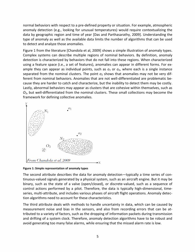
Figure 1 from the literature [Chandola et al, 2009] shows a simple illustration of anomaly types. Complex systems can describe multiple regions of nominal behaviors. By definition, anomaly detection is characterized by behaviors that do not fall into these regions. When characterized using a feature space (i.e., a set of features), anomalies can appear in different forms. For ex-ample they can appear as individual points, such as o1 or o2, where each is a single instance separated from the nominal clusters. The point o2 shows that anomalies may not be very dif-ferent from nominal behaviors. Anomalies that are not well-differentiated are problematic be-cause they are harder to catch and characterize, but the inability to detect them may be costly. Lastly, abnormal behaviors may appear as clusters that are cohesive within themselves, such as O3, but well-differentiated from the nominal clusters. These small collections may become the framework for defining collective anomalies.

Figure 1: Simple representation of anomaly types

The second attribute describes the data for anomaly detection—typically a time series of con-tinuous-valued signals generated by a physical system, such as an aircraft engine. But it may be binary, such as the state of a valve (open/closed), or discrete-valued, such as a sequence of control actions performed by a pilot. Therefore, the data is typically high-dimensional, time-series, multi-attribute, and includes various phases of aircraft flight operations. Anomaly detec-tion algorithms need to account for these characteristics.

The third attribute deals with methods to handle uncertainty in data, which can be caused by measurement noise and bias in the sensors, and also from recording errors that can be at-tributed to a variety of factors, such as the dropping of information packets during transmission and drifting of a system clock. Therefore, anomaly detection algorithms have to be robust and avoid generating too many false alarms, while ensuring that the missed alarm rate is low.

6

1.2 Machine Learning Methods

Machine learning approaches provide a basis for addressing data-driven anomaly detection problems. Supervised machine learning methods assume complete, or near complete, labeling of training data for building models to detect anomalies in nominal situations, and also for dif-ferentiating between different types of anomalies. Decision tree classifiers and neural networks are two examples of supervised anomaly detection methods.

Unsupervised methods apply to unlabeled data, and the corresponding algorithms are designed to discover groups or common patterns in the data. Clustering algorithms represent unsuper-vised methods that form groups of similar samples to divide up the data objects into a set of homogenous structures. An application of a clustering algorithm to typical flight data consisting of multiple sensor readings may discover groups of data, with the largest groups representing nominal behaviors. Once the nominal groups are represented by sensor ranges, diagnostic monitors can be designed to detect sensor values that are “out of range.” Further analysis of these out of range sensor readings by domain experts may result in the discovery and charac-terization of new anomalies or a more precise definition of known anomalies [Iverson, 2004].

A special form of unsupervised learning is called semi-supervised learning. Semi-supervised ma-chine learning methods need partial labeling of the data. They attempt to build models that dif-ferentiate between a known label, usually a majority class that represents nominal behavior, and “everything else,” which are labeled as outliers or anomalies. These models are tuned for specific behaviors and corresponding algorithms are designed to separate out the data points that do not fit with the majority data samples. Further analysis may be required to characterize and classify the specific anomalies [Das et al, 2011].

2 Anomaly Detection Methods

One of our primary objectives in this NASA Aviation Safety project is to develop a suite of su-pervised and unsupervised, data-driven, exploratory techniques to extend and enhance the di-agnostic and prognostic capabilities of the VIPR reasoner developed by Honeywell [Mylaras-wamy et al., 2011, Mack et al., 2012]. Supervised data driven methods were developed in Years 1 and 2 for robust, early detection of faults to minimize future occurrences of adverse events during flight. The approach employed labeled faulty data from the vicinity of the previous ad-verse event occurrences to learn tree-augmented naïve Bayes (TAN) structures. These struc-tures, when analyzed by experts, produced new approaches to improving reasoner perfor-mance by: (1) defining better thresholds for fault-detection monitors; (2) defining new moni-tors from existing sensor data; and (3) combining the output from multiple monitors to define “super monitors” that provided richer information to detect and isolate failure modes. The su-pervised learning approach, case studies based on the approach, and demonstration of the im-proved performance of VIPR reasoner with the improved reference models is discussed in [Mack et al 2012].

In contrast, our anomaly detection algorithms use a discovery or semi-supervised learning ap-proach to look at fleet-wide aircraft flight data to find situations where a flight segment or phase deviates from a nominal or baseline model derived from the data. The goal is to extend this empirical or data-driven approach to propose new condition indicators that complement

7

existing domain-expert developed monitors and monitors derived using the supervised learning methods [Mack et al 2012] to enable systematic study of the discovered anomalies. Further analysis of these anomalies by domain experts can lead to discovery of new fault conditions, such as those that arise from aircraft subsystem interactions and pilot-aircraft interactions that are hard to detect and slowly evolving faults across sequences of flights that may be detected by analyzing the fleet population. Confirmation of new discoveries can lead to definition of new condition indicators and updates to the VIPR reasoner to support system level diagnostics and prognostics.

In addition, study of fleet-wide data, creates opportunities for extending the study of equip-ment-related faults to anomalies that may be attributed to environmental conditions that could be weather-related or airport-related and pilot-related actions that influence aircraft behavior and flight trajectories in non-standard ways.

In the rest of this section, we briefly review unsupervised and semi-supervised methods that form the core of our data mining work in Year 3.

2.1 Unsupervised Anomaly Detection

Unsupervised methods are employed when we do not have sufficient initial knowledge for dif-ferentiating between nominal and anomalous behavior. This problem becomes even more sig-nificant when the data is high dimensional, making it hard for human experts to define precise classification labels or propose analytic methods for differentiating between nominal and anomalous data. In such situations, very little pre-knowledge about the data is assumed, and unbiased algorithms are employed to segment the overall data sets into groups, such that ob-jects within a group are more similar to each other than objects across groups. Groups that contain larger populations of the data objects are assumed to define nominal behavior, where-as the data objects that fall into smaller groups or fail to be labeled in any of the other groups (outliers) are defined to be anomalous. A number of generative modeling techniques may be employed to produce the nominal models. These techniques find an inherent structure in the data, using non-parametric algorithms that are distance or similarity-based and parametric al-gorithms that can be density-based or expectation maximization (EM)-based Bayesian methods.

Unsupervised detection methods will utilize the model output differently depending on wheth-er it exists as a Bayesian model of the evidence or through a number of clusters and cluster af-filiations. The easiest use of cluster output is to produce initial identifications of the data which are used as initial labels to produce a dataset for building models with supervised (and semi-supervised) techniques. This has been used with other anomaly detection techniques such as K-means and decision trees for chains of algorithms for anomaly detection [Gaddam et al, 2007]. For an expert, the clustering may serve as a pre-processing technique for organizing and further analyzing the data.

Clustering can also provide an unbiased mechanism for rejecting data previously defined as nominal because the clustering process derives groupings, and follow up expert analysis shows the groups are sufficiently different from each other. Depending on the methods used for clus-ter generation, the identified outliers may be interpreted differently. For example, a K-means algorithm may find anomalous groups, and additional analyses may find common feature signa-

8

tures for the group to define anomalous behavior [Bay and Schwabacher, 2003]. These signa-ture sets can also be used to define on board sensors that are used to track flight data and flag anomalies. Other examples of fault signature applications include intrusion detection [ Portnoy et al, 2001] where the signatures associated with different attacks are discovered instead of built by experts.

Density based clustering techniques have been used to discover lingering anomalies that fre-quently separate from nominal behavior groups [Li et al, 2011]. Unlike k-means, these outliers are not defined by signatures, but can be defined by probability distributions. Detection of anomalous situations may have to be performed by hypothesis testing schemes that compare two distributions.

A hierarchical clustering approach using a high cutoff threshold produces a small number of flattened clusters. As discussed earlier, large flattened clusters are labeled as nominal behav-iors, and the remaining groups and outliers are labeled as anomalous behaviors [Fu et al, 2005]. Hierarchical clustering provides additional opportunities for subdividing nominal and anoma-lous groups for further analysis.

Finally, a mixture of Gaussian clustering for anomaly detection can be found in multi-spectral image applications [Hazel, 2000]. Soft partitioning makes this clustering useful for environ-ments where data objects are distributed so that small numbers of features (compared to the whole) indicate the anomalies, but the number of objects with these feature values are mini-mal. Finding these clusters in data arising predominantly from normal behavior can make the discovery task difficult. Mixtures of Gaussians can be used to model the entire distributions over the data to discover these anomalies. Extensions can be used in conjunction with super-vised techniques such as ANNs to help identify abnormal patters in sea traffic [Laxhammar, 2008].

Density based clustering for anomaly detection was used in conjunction with feature reduction by principal component analysis (PCA) in [Rao, 1964]. The PCA produced a lower dimensional space with orthogonal features. Feature space reduction can apply to different types of clus-ters. PCA reduction can also be used with other unsupervised methods such as distribution test-ing to define general probabilistic neighborhoods of expected activity [Kwitt and Hofmann, 2007]. The testing will identify instances in the high-variance Eigen-space that are in the tail and thus anomalous, or outside the low-variance Eigen-space and therefore do not fit the distribu-tion of the data at all.

When generative models, such as Bayes nets are used for unsupervised learning, the class defi-nition, i.e., the joint probability distribution of a class can define a general classifier. New data instances are classified on the basis of this function, and then also serve to update the class def-initions. As an example, if one has to estimate abnormal vehicle paths for understanding poten-tial security risks. This approach requires deriving the general structure of a set of expected paths, and then examining the instances that do not conform to the set of known nominal paths. Once this structure is found, it can be leveraged to produce supervised structures that can form models on the attributes of the path and produce a model that possesses interpreta-ble properties about these anomalies [Mascaro et al, 2011].

9

Other methods in the unsupervised realm include sequence mining [Parthasarathy et al, 1999, Zaki, 2000], which are designed to find common subsequences in separate instances of the da-taset. These algorithms look for statistical support that can indicate when the different se-quences are significant in the data. Sequence mining has been used for unsupervised anomaly detection of aircraft anomalies [Budalakoti, 2009].

Often used in environments where the data is made up of symbolic sequences, more complex sequences that use numerical data may require complexity analysis [Broomhead and Kind, 1986; Keogh et al, 2007], to find anomalies inside the signal.

2.2 Semi-Supervised Anomaly Detection

Acquiring a labeled dataset of nominal and anomalous data objects is unlikely in many realistic applications. In such situations, the availability of a set of nominal data points may be sufficient to build reliable models, whereas the number of data points known to be anomalous may be too few (or none at all) to generate to generate reliable anomalous models. Therefore, the first step in semi-supervised anomaly detection may be to generate nominal models from nominal data, and compare new data objects against the nominal models. A good match implies that the new data object may be labeled as nominal, otherwise the data object is “anything other than nominal,” and, therefore, anomalous. This approach reduces errors by not over-classifying the anomaly (although misclassification as nominal is still possible).

Purely unsupervised methods that assume the data is unlabeled may generate class structures that are too forgiving of what constitutes nominal. In contrast, semi-supervised models that are derived from data labeled as nominal may become outdated for a specific environment. There-fore, it is important to use human experts who can detect when this happens and retrain the model with more appropriate and recent nominal data. In essence, when most of the opera-tions are nominal and identified as such by either the system, the expert, or through the use of unsupervised techniques, semi-supervised learning is useful for building the models of this be-havior and using this model to classify new data as nominal and anomalous.

The one-class Support Vector Machine (SVM) is a popular semi-supervised anomaly detection technique. It is used in diverse fields of anomaly detection such as diagnosis in aircraft [Das et al, 2011, Das et al, 2010], discovery of land mines [Nelson and Kingsbury, 2012], business appli-cations for churn models [Zhao et al, 2005] and like so many others, network intrusion detec-tion [Perdisci et al, 2006, Tran et al, 2004]. The one-class SVM is an extension of the SVM. The extension optimizes the classifier for a single class label. This optimization constructs a decision boundary around the training data to build a model that represents as much of the data as pos-sible. This technique, like its original construction, suffers from limited information for the ex-pert, and given a kernel transformation, it produces even less information. With a noisy training set, the decision boundary may be poor and may flag more anomalies than actually exist.

Other methods include the use of decision theoretic methods for applications like fraud detec-tion [Sharma and Panigrahi, 2012] in financial accounting and network intrusion [Lane, 2006]. Decision-theoretic methods are useful in the decision space of one class, where the structures for the classifier are built to isolate the single class. Unlike one-class SVMs, these methods are

10

more open to knowledge engineering tasks due to their openness. These can also be more time-consuming to build and potentially more brittle without a representative dataset.

Semi-supervised learning for anomaly detection can involve generative models such as mixtures models typically for network intrusion [Wang et al, 2006]. Generative models use the entire probability distribution from the data to determine probabilistically if an instance is either in the known class, or not. Bayesian networks also provide generative models for anomaly detec-tion and have been used to classify failures in computer equipment such as hard disks [Hamerly and Elkan, 2001]. Similar to decision theoretic methods, Bayesian networks are easier to apply for knowledge engineering. They can also be computationally more intensive than the one-class SVM.

2.3 Previous Work

General approaches to exploring the anomalous space and identifying specific anomalies are discussed in the literature. These approaches use a variety of learning algorithm, such as least-squares regression [Bishop, 2007], a supervised learning method that derives discriminative models using simple error minimizations techniques. This approach produces robust algorithms for additive faults. Receiver Operating Characteristics (ROC) curves can be used to tune the de-tection algorithms and set the false alarm rates to desirable values [Chu et al, 2010]. However, least squares ad similar approaches require large amounts of labeled data to generate detec-tors that are truly robust and globally valid. Detailed knowledge of human experts is also re-quired to tune the false positive and false negative rates based on the nature of the anomaly, and the phase of operation.

Multiple kernel anomaly detection (MKAD) is a semi-supervised method for anomaly detection [Das et al, 2011, Das et al, 2010]. The algorithm first preprocesses all continuous sequential da-ta (for example, the time series features of the flight data) into symbolic feature sequences, so that a symbol-based measure can be applied for computing the similarity between two tem-poral samples. The similarity metric is based on a measure that computes the longest common subsequence between the two strings, and is known as the normalized longest common subse-quence (nLCS)[ Budalakoti et al, 2006]. This measure is most effective when sequences (wheth-er discrete or continuous) can be transformed into discrete sequences with a small symbolic al-phabet. As we discovered in our work with flight data, this transformation may be an important challenge and hard to accomplish without loss of significant information relevant to anomaly detection.

Once the pairwise similarity measures are obtained across all features that represent the data samples, a kernel is constructed as a One-Class SVM classifier [Ratsch et al, 2000]. The assump-tion is that the SVM is constructed from nominal data, and, therefore, can be used to discrimi-nate between nominal and non-nominal, i.e., anomalous data. The overall approach defines a semi-supervised process. All data samples classified as anomalous by the SVM are analyzed separately after classification using other methods, since the kernels defined by the SVM model are difficult to interpret semantically to define the nature of the anomaly. The MKAD approach has been applied to a combination of switching and continuous FOQA data for a fleet of aircraft [Das et al, 2011]. Its models are shown to derive some interesting anomalies, such as a high en-

11

ergy approach landing, human (pilot) responses to environmental disturbances, and high speed low altitude flights.

In contrast, SequenceMiner [Budalakoti et al, 2009] also focuses on a set of feature sequences across multiple samples and uses the nLCS metric but takes an unsupervised approach to con-structing its model. Using clustering, SequenceMiner attempts to find groups with similar nLCS values. Once clusters have been defined, data points outside the cluster boundaries typically represent outlier values that can be isolated for further analysis by human experts. The cluster models can indicate which features contributed to the outlier values, which makes the task of anomaly labeling and definition much easier for human experts. SequenceMiner also applies a genetic algorithm to compute missing and extra symbols in the anomalous data, providing the user with even more information on the nature of the anomaly. The algorithm can be used for discovery as well as analysis. MKAD uses a SequenceMiner routine on the group of anomalies flagged in the test set to better understand why these samples were detected.

The nLCS metric can be considered to be a dimensionality reduction or data compression scheme, where continuous or discrete-valued data is compressed into a small number of inter-vals to simplify the comparison process for time series data. Other methods that use similar techniques include Morning Report [Chidester, 2003], which builds a statistical signature across each feature sequence to describe its information content in a lower dimensional space. Dis-tance metrics, such as the Mahalanobis distance, are employed to distinguish data samples, e.g., flights, that are sufficiently removed (specified by a pre-defined threshold or a statistical test) from the majority of the samples, and are classified as outliers. Much like MKAD, Morning Report requires a second pass on the outliers to characterize and classify them as specific anomalies.

Techniques are available for combining information across a sample’s features to reduce the sample’s dimensionality, but do not explicitly look for information about the sequences. Orca [Bay and Schwabacher, 2003] uses a scalable k-nearest neighbor approach to detect anomalies in data with continuous and discrete features. Outlier detection is also based on a k-nearest neighbor analysis, but since each data point is treated as independent, the algorithm cannot detect anomalies with temporal signatures.

Inductive monitoring system (IMS) is a distance-based anomaly detection method that analyzes continuous-valued features without transforming them into a symbolic form [Iverson, 2004]. The method uses an incremental cluster analysis approach to build models of expected opera-tion of the system, but also does not consider the temporal patterns in the data. The Euclidean distance from an outlier data point to the nearest cluster center is reported as the anomaly score for that data point. This method was originally designed to deal with flight data, where new monitors for anomaly detection could be built using models of the clusters and the Euclid-ean measures.

Another method that ignores temporal information combines principal component analysis (PCA) for dimensionality reduction (or data compression) and density-based clustering (DBSCAN) as an unsupervised method for classifying the data into nominal and anomalous sets [Ester and Kriegel, 1996; Li, et al, 2011]. This method relies on “unrolling” the sample so that every time series feature is converted into a set of features, one for each time point in the se-

12

quence (this requires all samples to be the same temporal length to create a rectangular da-taset). These “unrolled” samples are projected into a lower dimensional space that corresponds to the selected eigenvectors that are derived using a PCA analysis. This projection creates a re-duced and orthogonal feature space to which density-based clustering is applied to group the data into different classes. The advantage of this approach as compared to the methods de-scribed above is that it requires little domain knowledge to set the input parameters, and the algorithm is efficient for large datasets. The clusters generated by the algorithm can be of arbi-trary shape (unlike k-means, which generates hyper-spherical clusters), and the algorithm is ro-bust to noise in the data. Another advantage of DBSCAN is that outliers can be defined by prob-ability distributions, which may be a more robust measure than straight distance metrics. The output of this method produces clusters that are homogeneous in the chosen feature space, and a set of outlier data points that become the focus of further investigation. Like the earlier methods, further analysis is required by human experts to characterize and define anomalies. Table 2 compares and contrasts the methods.

Table 2: Analysis methods for anomaly detection

Our approach to anomaly detection follows a similar structure to the methods defined above. The overall goal, as stated earlier, is to use existing fleet-wide flight data to discover, character-ize, and classify anomalies. Anomalies may be considered to be situations that deviate from nominal operations, which can have multiple causes, including: equipment-related, environ-ment-related, and pilot actions. Since we do not have access to sufficiently broad and detailed nominal models of flight operations, we have to adopt a two-part approach: Step 1 is per-formed offline and uses unsupervised learning methods to establish a baseline nominal model. Step 2 is performed online on a sequence of flights for individual aircraft in the fleet and uses a simplified, approximate version of the baseline model to capture flight operations that deviate from the baseline nominal; as part of this analysis this step also establishes the flight features that are primary contributors to the anomaly.

This data collected over multiple flights of multiple, but identical aircraft, is again analyzed by human experts at the fleet level, i.e., across flights to detect and characterize anomalies from aircraft safety and performance viewpoints, and this may lead to the definition of new diagnos-tic monitors, and new faults that are used to update the system reference models. Some of the monitors may also form new prognostic monitors that capture richer data to assist aircraft

Features

Multiple Kernel Anomaly

Detection (MKAD) PCA-Based Cluster Analysis Inductive Monitoring System (IMS) SequenceMiner

Labeling Semi-Supervised Unsupervised Semi-Supervised UnsupervisedTemporal

Sequence

or IID Sequence IID Sequence SequenceDiscrete or

Continuous Both Both Both BothProcess

Continuous

Into

Discrete Yes-SAX Yes-SAXFeature

Reduction YesBase

Algorithm One-Class SVM PCA Clustering ClusteringSecond

Algorithm Density Based Clustering Distance Calculation

13

maintenance operations. The offline and online analysis methods are described in greater detail in the next section.

3 Anomaly Detection Approach

Focusing our general discovery approach on an aircraft operations viewpoint, the anomaly de-tection task within VIPR, results in monitoring individual aircraft flights by collecting and pro-cessing onboard data and continuously looking for emerging patterns. These steps are illustrat-ed in Figure 2 and can be summarized into two phases, described below.

Figure 2: Operational steps in VIPR anomaly detection

1. Pre-analysis or the discovery phase: This phase sets up the anomaly detection function within VIPR.

a) The primary task is to establish a baseline of nominal operations from historical fleet data.

b) A secondary task is to characterize fleet-wide anomalies, i.e., anomalies whose fre-quency of occurrence exceeds a pre-defined threshold in the historical data, charac-terize and analyze these anomalies with expert help, and incorporate detection and isolation of these anomalies into the VIPR reference model, especially if they are re-lated to safety and performance of aircraft.

2. Post Analysis: This phase uses a version of the baseline nominal model online to contin-ually generate anomalies and translate the condition indicators related to the ones con-sidered significant by experts into VIPR monitors to enhance prognostic reasoning.

a) If a pattern is an outlier when compared to a pre-established baseline, it is download-ed from the airplane as an anomaly report to a central location for further analysis.

b) An expert analyzes a series of anomaly reports and determines their significance with respect to operational practices, safety hazards, and/or equipment related malfunc-tions.

c) A subset of these cases deemed important to aircraft safety or operational efficiency is programmed and deployed across the entire aircraft fleet as new VIPR monitors.

From a functional point of view within the VIPR context [Mylaraswamy et al., 2011], a diagnos-tic/prognostic monitor provides evidence towards the presence of specific failure modes—

14

called its ambiguity set. Ambiguity set indicates that the evidence provided by a D/P monitor may not map to exactly one failure mode. Nevertheless, all failure modes associated with a D/P monitor are actionable through appropriate maintenance or mitigation actions.

Anomaly monitors, on the other hand, do not have a pre-defined ambiguity group. In fact, the overall objective of the anomaly detection function within VIPR is to define this ambiguity group.

3.1 Establishing a baseline: Offline Analysis

The offline approach to deriving the baseline nominal model that forms the basis for online anomaly detection (i.e., detection of anomalies during flight) is based on an unsupervised learn-

ing approach. The overall approach involves the following steps, which are also marked 15 in Figure 3.

Figure 3: Establishing a baseline -- offline unsupervised analysis

1. Data frames from individual aircraft surrounding key flight phases such as taxiing, take-off, cruise, descent, and touch down are collected over a significant period of time (e.g., years) from an operating fleet. This forms the baseline data for anomaly detection studies1. Each data frame is a two-dimensional vector, and each flight defines a unique data point. There-

fore, a set of flights, define a P N M data cube, where P is the number of flight seg-

1 Subsets of this data were also used for our supervised learning methods for improving detection accuracy of

known faults.

15

ments, N is the number of features associated with each flight segment, and M is the num-ber of samples that define the time-varying characteristic of a feature. Here, the term “fea-ture” is synonymous with an aircraft sensor parametric value. Pairwise feature distances be-tween every pair of data points are computed using the Kolmogorov complexity measure [Keogh et al, 2007[. This computation requires O(P2N) calculations, which can be computa-tionally intensive, because P is typically of the order of 104 to 105 and N is typically of the order of 103 (see Table 1).

2. The pairwise feature dissimilarities between flight segments are converted to a two-dimensional matrix of pairwise distances among flight segments.

3. The Euclidean metric is employed for building the two-dimensional dissimilarity matrix among flight segments.

4. A hierarchical clustering approach (in our case, we used the complete link clustering algo-rithm) is used to generate the dendrogram that forms the basis for defining the nominal clusters of flight segments as well as the outliers and anomalous clusters.

5. At this stage, offline analysis bifurcates to: (a) extract a nominal model to be employed for on-aircraft anomaly detection (Steps 2 – 4 in Figure 3), and (b) an anomalous clusters that can be used directly to generate VIPR monitors as described in Section 3.2.2).

In the remainder of this section, we describe the salient features of each step in greater detail.

3.1.1 Complexity Measures

Kolmogorov complexity [Keogh et al, 2007] defines the complexity of a signal (a string of values) as the smallest Turing machine that can reproduce that signal [Kolmogorov, 1965]. Modeling more complex signal patterns will obviously require longer program segments. Repeating pat-terns would be represented using constructs, such as loops, but this keeps the length of the program short. This approach may be used as an absolute metric for signal complexity, since Turing machines can simulate any program, and thus provide a measure that is universally ap-plicable.

However, this theory is difficult to realize, since Turing Machines are a theoretical construct, and methods to compute the Kolmogorov-Complexity would be intractable. More precisely, given a signal whose complexity measure needs to be calculated, a universal Turing machine must test the decision space of other Turing machines to decide if they can accurately repro-duce the input. Once the space has been searched, the smallest program’s length would be cal-culated and returned as output. This is fundamentally a search for machine correctness through all possible computational machines (or even a large subset, given some initial pruning). Run-ning a program to detect another’s correctness (and establish that it will complete) is the halt-ing problem, which is undecidable. Even if the conditions for checking a given machine are re-laxed, this is an intractable problem, given the decision space of possible programs. As a practi-cal alternative, researchers have specified ways to approximate this value. One of the primary methods utilizes compression algorithms for strings as the measure for complexity. A class of approaches called lossless compression algorithms, are designed to reduce data sequences to a form where they have the smallest memory footprint (similar to the n-FSR method above), but an inverse algorithm can restore them to their original form without any loss of information through the compression and decompression processes. The more repetition a signal has, the

16

more it can be compressed (by using of loop logic). The memory footprint of a signal after com-pression can be used as an approximate measure of the complexity for that signal.

Given, a compression algorithm chosen by the practitioner, the compression measurements are combined across different features to define a dissimilarity measure between pairs of data ob-jects. Not all compression measures result in dissimilarity measures that have metric properties (i.e., they satisfy the triangle inequality). We take this into account in subsequent discussions.

Due to the nature of different signals, generic choices for both compression algorithm and dis-similarity calculations may produce very different results. As an initial step, we start with well-known and widely-used classes of compression algorithms, such as the DEFLATE Deutsch, 1996], Lempel-Ziv algorithms [Sayood, 2000], and Markov chain-based algorithms [Merhav et al, 1989]. However, a compression algorithm that captures the right information from the data using a minimal representation more accurately satisfies the Kolmogorov-Complexity approxi-mation, since it is better at defining the smallest amount of information required to build the string. Finding the best compression algorithm for different types of signals will be addressed in this work to best utilize compression-based complexity measures.

3.1.2 Complexity Experiments with Compression Based Approximations of Kolmogorov-Complexity

The number of different ways in which we may compute an approximation of the Kolmogorov Complexity of a signal is the Cartesian product of the distance measures and the compression algorithms we employ for these analyses. Different compression algorithms may be better suit-ed to different signals, and different distance measures are more sensitive to the relevant varia-tions that we want to capture about these signals. Note that in the aircraft flight data, we are dealing with a mix of continuous signals, such as velocity or the aircraft, or temperature of the engine that are physical variables, defined by dynamic physical processes, and discrete signals, such as a sequence of actions that the pilot may employ during the take-off phase of a flight. In this work, we are developing schemes for studying the measures that provide adequate results for compression time series signals for features into a smaller set of values, and corresponding measures that define the similarity or dissimilarity between two sets of values for the same fea-ture. The work reported here is preliminary, but having made choices on compression algo-rithms and distance measures, we run a set of empirical experiments to compare the choices, and establish those that are most compatible with our anomaly detection framework.

As discussed, our compression algorithms are lossless, but the aircraft signals may be noisy, so it is important to test the robustness of the measures that we employ, along with other proper-ties, such as monotonicity and scalability. The baseline compression algorithm will be the DE-FLATE family of algorithms, with an implementation known as DZIP. We will also run experi-ments using the Lempel-Ziv compression family of algorithms, specifically LZW (used in GIF im-age compression) [Sayood, 2000; Merhav et al, 1989]. A third choice is the PPM (prediction by partial matching) [Zhang and Adjeroh, 2008] scheme, which uses probabilistic methods to help find the most common repeated values and then use smaller number of bits to represent them. Our final compression algorithm is the Burrows-Wheeler transform (BWT), which uses a sorting algorithm as a base step in the compression.

17

Let x and y be two strings. A chosen compression function C is used by measuring the number of bytes after compression. We represent this by starting with the basic compression of either x or y, i.e., C(x) or C(y). Other measurements include C(xy), which is the compression of the con-catenation of string x and string y, and C(x|y), which is the compression of x, using the com-pression profile of y.

These algorithms will be used with two distance measures. These measures are the Normalized Compression Distance (NCD) [79] and the Complexity-Invariant Distance Measure (CiDM) [4]. NCD is a metric, when the Compression algorithm satisfies Compression(x) = C(xx) within loga-rithmic bounds. NCD measures the dissimilarity as

( ) ( ) * ( ) ( )+

* ( ) ( )+

The values for NCD are bounded by the interval [0,1], where 0 means the signals are identical and 1 means that they are completely dissimilar. The difference between NCD and CDM when these measures are expanded is the choice for the denominator. In NCD, the denominator normalizes the value to give a bound that can start at 0 (and it also satisfies the triangle ine-quality). The NCD has been shown to be effective for clustering applications [Cilibrasi and Vitanyi, 2005].

The CiDM was built for time series data, and instead of using only compression to find the dis-similarity, CiDM uses compression as a way of normalizing the Euclidean distance(ED). The CiDM is defined as:

( ) ( ( ) * ( ) ( )+)

* ( ) ( )+

The values for this measure will reflect a distance that is invariant to amplitude difference, off-set of the signals, and local scaling. This measure provides an alternative to a purely compres-sion based dissimilarity measure.

We use three different types of signals to explore the different combinations of compression and distance measures. These three are linear, quadratic and sinusoid functions. For each func-tion, we vary a number of the parameters. For linear functions, represented by the function, we vary both the slope, b, and the y-intercept, c. The quadratic function, has 3 possible parameters to vary, a, b, and c. To keep the experiments roughly equivalent, we vary the coefficient of the x^2 term and the x term. For the sinusoid function, ( ) we vary the frequency term, and the offset, . Each parameter is assigned one of the following values: [1, 10, 50, 100, 500], producing 25 different signals for each function. To focus on the pure implications, the current experiments are with noise-free signals. In the future, we will extend this work studying the effects of these measures on noisy signals.

For the 75 ( ) signals, a pairwise distance is computed using each of the combinations of the measures and the compression algorithms. These distances are then examined in two dif-ferent ways. First, we examine classification accuracy, using a one nearest neighbor (1-NN) clas-sifier and the base signal type (linear, quadratic and sinusoid) as the class types. Secondly, we

18

examine each signal type in terms of the pairwise distance values between pairs of signals of the same type determining the sensitivity of the signal parameters to the distance computa-tions, and also look at the distance measures between different signal types. This allows us to start investigating how effective these measures are in response to both the shift parameter (example: a constant slope, but changing y-intercept for linear signals), with the scale parame-ter (e.g., increasing slope values for a linear signal with the y-intercept held constant).

The classification of these signals across the different 8 different algorithms was all quite high. The NCD measure with DZIP, LZW, and BWT each misclassified two of the 75 signals, for a 97.3 percent overall accuracy. PPM was the worst of the compression measures, misclassifying 10 of the signals, for an overall accuracy of 86.67%. Of note, the LZ77, LZW, and BWT each misclassi-fied the same two samples, the Linear signal with a slope of 500 and an offset of 500 was classi-fied as a quadratic function and the quadratic function with the form 500x^2+500x + 1 was clas-sified as Sinusoid. The PPM on the other hand made 9 misclassifications in the linear samples, each of them were misclassified as quadratic signals, and the same quadratic sample as above was also misclassified with PPM.

The CiDM classification was overall more consistent with PPM and BWT, both showing 100% accuracy with this measure. DZIP misclassified a single instance for 98.67% accuracy (a quadrat-ic function was labeled as linear). LZW also misclassified a single instance, labeling a linear func-tion as a sinusoid.

It's clear from these experiments that in the presence of zero noise, both measures are fairly accurate, with CiDM slightly better. Perhaps more interesting was that PPM was a poor choice for NCD, but had perfect accuracy with CiDM. Looking at the misclassifications for each pro-vides insight into which functions these measures struggle to separate. NCD appears to have is-sues when the parameter, specifically the slope for linear and the parameter for x^2 grow large, as both tend to be misclassified as quadratic and sinusoidal signals, respectively. For CiDM on the other hand, the two mistakes were both a quadratic and sinusoid being classified as a linear function.

Looking at the varying parameters of signals and how the distances change tells us how these measures may be used in anomaly detection, and specifically, how sensitive these measures are to different effects. Distance values with relation to shift in the signal are important. For exam-ple a takeoff may be slightly early, or slightly late, than normal but possess the same type of take-off, this wouldn't normally be an anomaly(unless it was very early, or very late), meaning that for the most part, there should be little changes in the shift.

Looking at the two signals that feature a shift (linear with a y-intercept and sinusoid with a shift parameter), we find that they each react differently. For sinusoid signals as in Figure 4, both dis-tance measures produce constant results for a given compression algorithm. In fact, CiDM is agnostic of compression algorithm and produces a 0 value indicating complete similarity when we vary the shift, but not the frequency.

19

Figure 4: Sinusoidal Function Comparison Phase Change: CiDM measure

When we examine the NCD values, we found that the value, will depend on the compression algorithm, but without reservation also remains constant for no matter the frequency. This can be seen in Figure 5 with NCD and BWT Compression. From both of these results we can con-clude that with repeating information such as that seen in a sinusoid, but with perhaps a frame offset, these measures could be invariant to that difference.

Figure 5: Sinusoidal Function Comparisons Phase Change: NCD measure, BWT compression

The linear case however is not quite as simple. Of note, both measures have the same results, which is to be expected, since there is no repeating of information such as a sinusoid, rather the values are all offset by a single value. For NCD, we see that there is a matter of which compres-sion algorithm you use. For example, in Figure 6 is NCD with the DZIP algorithm for a slope of 1, and shifting values for the y-intercept. It slowly grows until the y-intercept is 100 to 500, when

0

0.1

0.2

0.3

0.4

0.5

0.6

0.7

0.8

0.9

1

(1,10) (1,50) (1,100) (1,500)

CiDM on Sinusoid Function Comparsions: Base

signal: = 1, = 1

(1,1)

0

0.1

0.2

0.3

0.4

0.5

0.6

(1,10) (1,50) (1,100) (1,500)

NCD with BWT Compression on a Sinusoid

Function: Base signal: = 1, = 1

(1,1)

(, )

(, )

20

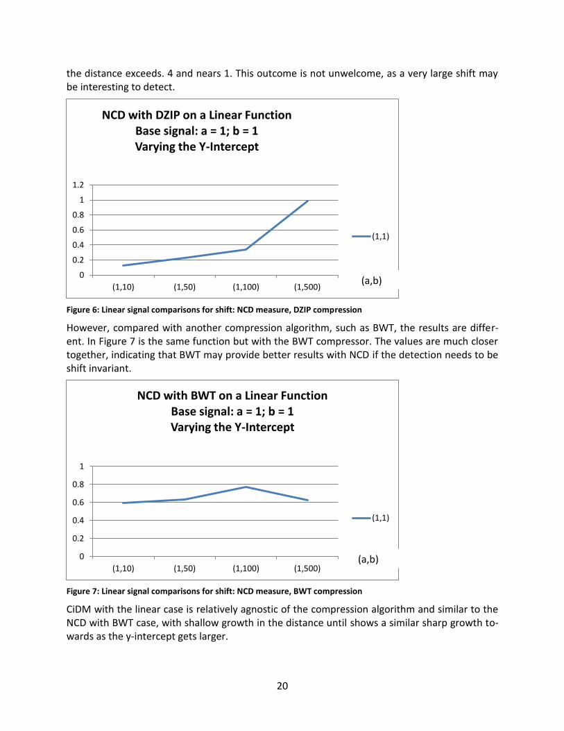
the distance exceeds. 4 and nears 1. This outcome is not unwelcome, as a very large shift may be interesting to detect.

Figure 6: Linear signal comparisons for shift: NCD measure, DZIP compression

However, compared with another compression algorithm, such as BWT, the results are differ-ent. In Figure 7 is the same function but with the BWT compressor. The values are much closer together, indicating that BWT may provide better results with NCD if the detection needs to be shift invariant.

Figure 7: Linear signal comparisons for shift: NCD measure, BWT compression

CiDM with the linear case is relatively agnostic of the compression algorithm and similar to the NCD with BWT case, with shallow growth in the distance until shows a similar sharp growth to-wards as the y-intercept gets larger.

0

0.2

0.4

0.6

0.8

1

1.2

(1,10) (1,50) (1,100) (1,500)

NCD with DZIP on a Linear Function Base signal: a = 1; b = 1 Varying the Y-Intercept

(1,1)

0

0.2

0.4

0.6

0.8

1

(1,10) (1,50) (1,100) (1,500)

NCD with BWT on a Linear Function Base signal: a = 1; b = 1 Varying the Y-Intercept

(1,1)

(a,b)

(a,b)

21

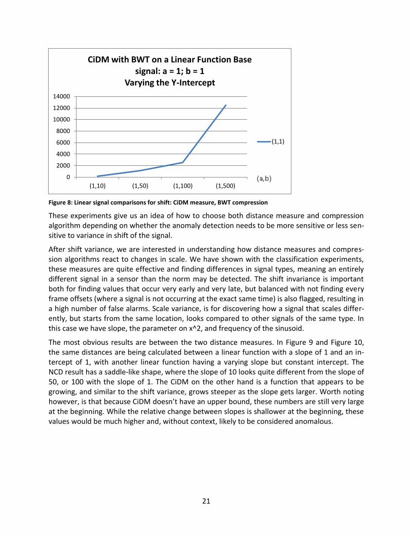
Figure 8: Linear signal comparisons for shift: CiDM measure, BWT compression

These experiments give us an idea of how to choose both distance measure and compression algorithm depending on whether the anomaly detection needs to be more sensitive or less sen-sitive to variance in shift of the signal.

After shift variance, we are interested in understanding how distance measures and compres-sion algorithms react to changes in scale. We have shown with the classification experiments, these measures are quite effective and finding differences in signal types, meaning an entirely different signal in a sensor than the norm may be detected. The shift invariance is important both for finding values that occur very early and very late, but balanced with not finding every frame offsets (where a signal is not occurring at the exact same time) is also flagged, resulting in a high number of false alarms. Scale variance, is for discovering how a signal that scales differ-ently, but starts from the same location, looks compared to other signals of the same type. In this case we have slope, the parameter on x^2, and frequency of the sinusoid.

The most obvious results are between the two distance measures. In Figure 9 and Figure 10, the same distances are being calculated between a linear function with a slope of 1 and an in-tercept of 1, with another linear function having a varying slope but constant intercept. The NCD result has a saddle-like shape, where the slope of 10 looks quite different from the slope of 50, or 100 with the slope of 1. The CiDM on the other hand is a function that appears to be growing, and similar to the shift variance, grows steeper as the slope gets larger. Worth noting however, is that because CiDM doesn’t have an upper bound, these numbers are still very large at the beginning. While the relative change between slopes is shallower at the beginning, these values would be much higher and, without context, likely to be considered anomalous.

0

2000

4000

6000

8000

10000

12000

14000

(1,10) (1,50) (1,100) (1,500)

CiDM with BWT on a Linear Function Base signal: a = 1; b = 1

Varying the Y-Intercept

(1,1)

22

Figure 9: Linear signal comparisons for scaling: NCD measure, DZIP compression

Figure 10: Linear signal comparisons for shift: CiDM measure, DZIP compression

One last observation is how this change is magnified in the scope of the quadratic function. As seen in Figure 11 with CiDM (with the more predicatable shape), when the scale occurs with a larger term, such as x^2, the growth, while similar in abstract shape to the linear case is much larger. This helps validate that, while CiDM was more accurate in terms of classification, in terms of tracking the impact of scale variance, CiDM reacts similarly in both cases.

1.01

1.015

1.02

1.025

1.03

1.035

1.04

1.045

1.05

(10,1) (50,1) (100,1) (500,1)

NCD with DZIP on a Linear Function signal: a = 1; b = 1 Varying the Slope

(1,1)

0

1000000

2000000

3000000

4000000

5000000

6000000

7000000

(10,1) (50,1) (100,1) (500,1)

CiDM with DZIP on a Linear Function signal: a = 1; b = 1 Varying the Slope

(1,1)

23

Figure 11: Quadratic signal comparisons for scaling: CiDM measure, DZIP compression

Table 3: Results from experimental Studies

Signal Template

Distance Measure

Co

mp

ress

ion

Alg

ori

thm

s

NCD CiDM

Monotonicity* Sensitivity* Monotonicity* Sensitivity*

DZIP Linear N, N -, - Y, Y 2, 2

Quadratic Y, N -, - Y, Y 2, 2

Sinusoid Y, Y 3, O N, Y -, O

LZW Linear Y, N 1, - Y, Y 2, 2

Quadratic Y, Y -, 1 Y, Y 2, 2

Sinusoid N, Y -, O N, Y -, O

PPM Linear N, N -, - Y, Y 2, 2

Quadratic N, N -, - Y, Y 2, 2

Sinusoid Y, Y 2, O N, Y -, O

BWT Linear N, N -, - Y, Y 2, 2

Quadratic N, N -, - Y, Y 2, 2

Sinusoid Y, Y 1, O N, Y -, O * Column 1: Scaling, Column 2: Shift

Table 3 summarizes the results of these experiments. For the eight combinations of distance measure and compression algorithms, we examined how the following properties changed as we varied the parameters associated with the three template signals.

1. Monotonic: This property measures how the distance changes as the signals scales and shifts from the baseline template. Monotonicity is labeled either with a N (not monoton-ic) or with a Y (monotonic).

0

500000000

1E+09

1.5E+09

2E+09

(10,1) (50,1) (100,1) (500,1)

CiDM with DZIP on a Quadratic Function signal: a = 1; b = 1

Varying the X^2 (a) Param

(1,1)

24

2. Sensitivity: This property measures how the monotonity changes as we vary the parame-ters of the shapes to generate family of linear/quadratic/sinusoids. Ideally we want the

metric to be sensitive to the “magnitude” of the signal. Sensitivity is marked with a “” when we could not establish any definitive statement. Sensitivity has an “O” when the function was monotonic, but did not change when the templates were shifted and scaled. Lastly, the Sensitivity is ranked with the larger number meaning the sensitivity over the course of the distances was larger.

In Table 3, for each signal template, we calculated the listed properties under two conditions: (a) scaling- a new signal was generated by multiplying the template by , and (2) shifting – a new signal was generated by adding to the template. From these experiments we draw the following conclusions:

1. For linear and quadratic signals templates, CiDM is the better distance measure and seems to be independent of the compression algorithm.

2. For sinusoids, shifting the template has no effect for both NCD & CiDM distance measures irrespective of the compression algorithm used.

3. For sinusoids, NCD distance was affected both by a shift and scaling of the template, irre-spective of the compression algorithm used.

4. DZIP seems to be the compression algorithm of choice, followed by PPM, and then BWT.

Other complexity measures that do not rely on compression may also be considered in future work, especially if they have better monotonicity and sensitivity properties.. These measures include autoregressive model order estimation (AR order estimation), wavelet transformations, and approximate entropy (ApEn). AR order estimate [S. Rezek, 1998] measures the complexity in a signal by the number of coefficients (i.e., the order of the regression function) in the poly-nomial function model of the temporal signal that minimizes the mean square error estimate [S. Kay and S. Marple, 1981]. Wavelet transforms are selected as complexity metrics because when they are applied to continuous-time signals (both discrete and continuous), the transform returns sets of scaled components that define each signal. ApEn [R. Hilborn, 1994], [S. Pincus, 1995] is designed to compute the approximate entropy in a signal. Entropy is a probabilistic measure from information theory linked to information gain or information content.

3.1.3 Computing Pairwise Flight Dissimilarities: Euclidean Metric

Given the complexity measure and distance metric calculated between each feature in the frame and each aircraft, the next step is to compute the pairwise distance between flight seg-ments from individual feature differences. Typical distance metrics include the Manhattan, Eu-clidean, Mahalanobis, and Minkowski metrics. We used the standard Euclidean metric as the distance measure. Here, since each value is already a distance for a given sensor between two flights, a square root of the dot product of all the distances will produce a single distance be-tween the two flights.

25

3.1.4 Unsupervised Learning: Defining the Baseline Model

Using the Euclidean metric to flatten the distances to a single matrix, a hierarchical clustering algorithm (either complete link or the unweighted pair group method with arithmetic mean (UPGMA)) will be employed to construct dendrograms from this dissimilarity matrix. Complete link clustering joins two clusters together only if the furthest distance between any two points in the clusters is the smallest distance value remaining in the adjacency matrix. The dendro-gram will help further classify and characterize nominal data from anomalies by grouping [A. K. Jain and R. C. Dubes, 1998] the different flights together. Separating out the nominal from the-se anomalous clusters will isolate different sets of data. The nominal patch can be used to con-struct a baseline set of data for further analysis and to be used in an online algorithm during flight.

3.2 Anomaly Generation during Flight: Online Analysis

The result from the offline expert analysis helps determine the significance of the anomaly. From an operational point of view, significance implies that the anomaly affects operational, safety, or equipment maintenance, and most importantly, an appropriate mitigation or mainte-nance action can be defined for the next time this pattern occurs.

Functionally, within VIPR the failure modes provide this logical abstraction, which when assert-ed by a fault condition, enables the flight crew to avoid a safety incident or helps the maintain-er execute a condition-based maintenance action. This failure mode set {F} is defined within the VIPR static reference model, which is loaded externally as a loadable data image (LDI). If such an appropriate failure mode already exists in the VIPR static reference model, the newly-defined anomaly pattern can provide more evidence as additional diagnostic or prognostic monitors. If an appropriate failure mode does not exist, then we may need to create a new fail-ure mode node in the static reference model.

Procedurally, anomaly detection reduces to adding more nodes to the evidence set {E} or add-ing more nodes to the failure modes set {F}, adding more arcs to the bipartite graph, and as-signing a detection probability. This step is called reference model authoring. Functionally, it creates a delta-increment to the existing static reference model. This delta-increment appends additional information to the VIPR LDI and can be uploaded to every aircraft in the fleet during a regular software update cycle.

These functional steps can repeat several times in response to the detection of novel anoma-lies. The process begins with the generation of anomaly monitors that are eventually translated to on-aircraft diagnostic and prognostic (D/P) monitors. These D/P monitors, viewed as incre-ments to the on-aircraft VIPR reference model, are used by the reasoner algorithm to generate plausible hypotheses of fault conditions that may cause adverse safety incidents or trigger con-dition-based maintenance.

Next, we describe an architecture to realize this VIPR function as an extension to the current aircraft condition monitoring function (ACMF).

26

3.2.1 The Onboard Anomaly Detection Scheme

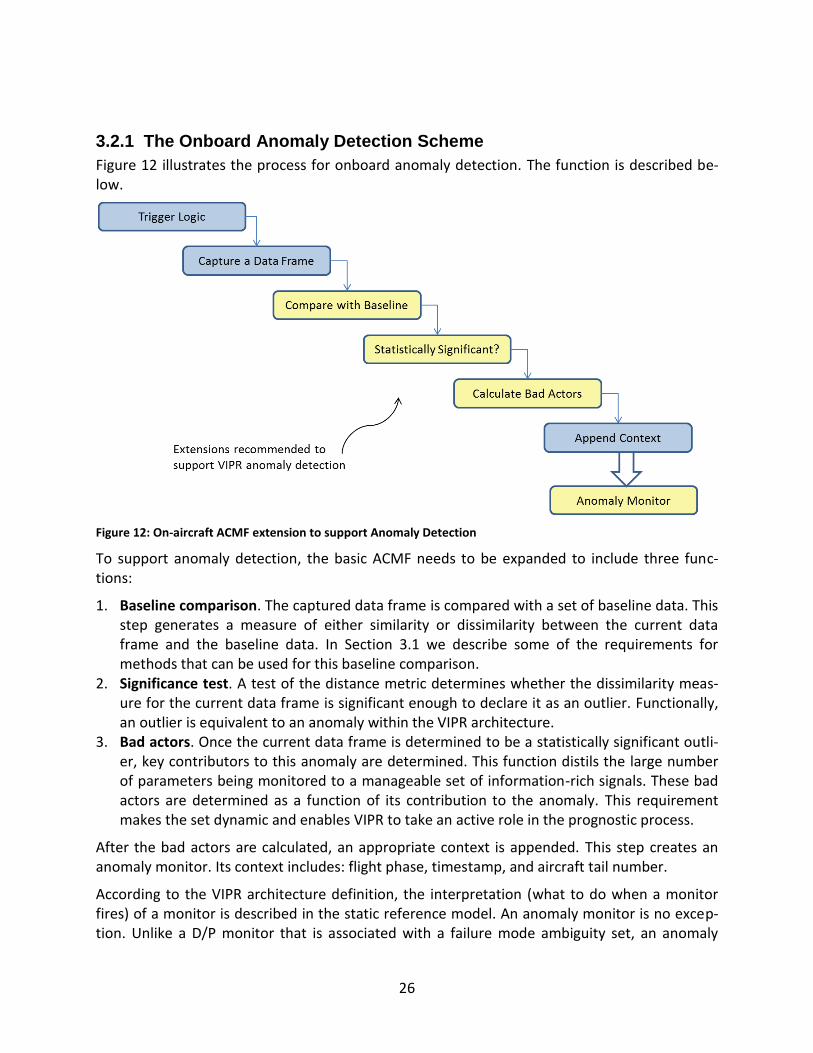
Figure 12 illustrates the process for onboard anomaly detection. The function is described be-low.

Figure 12: On-aircraft ACMF extension to support Anomaly Detection

To support anomaly detection, the basic ACMF needs to be expanded to include three func-tions:

1. Baseline comparison. The captured data frame is compared with a set of baseline data. This step generates a measure of either similarity or dissimilarity between the current data frame and the baseline data. In Section 3.1 we describe some of the requirements for methods that can be used for this baseline comparison.

2. Significance test. A test of the distance metric determines whether the dissimilarity meas-ure for the current data frame is significant enough to declare it as an outlier. Functionally, an outlier is equivalent to an anomaly within the VIPR architecture.

3. Bad actors. Once the current data frame is determined to be a statistically significant outli-er, key contributors to this anomaly are determined. This function distils the large number of parameters being monitored to a manageable set of information-rich signals. These bad actors are determined as a function of its contribution to the anomaly. This requirement makes the set dynamic and enables VIPR to take an active role in the prognostic process.

After the bad actors are calculated, an appropriate context is appended. This step creates an anomaly monitor. Its context includes: flight phase, timestamp, and aircraft tail number.

According to the VIPR architecture definition, the interpretation (what to do when a monitor fires) of a monitor is described in the static reference model. An anomaly monitor is no excep-tion. Unlike a D/P monitor that is associated with a failure mode ambiguity set, an anomaly

27

monitor does not have this information. Hence, it cannot create a new fault hypothesis and participate in the prognostic reasoning process directly. However, an anomaly monitor enables VIPR to take an active part in detecting the onset of adverse events or equipment malfunction through the offline expert analysis.

To enable adverse event detection, VIPR’s system reference model must be expanded to in-clude “what to do when an anomaly monitor” fires. That is, the system reference model sche-ma needs to be expanded to encode this information. From our current work, we propose the following to additions to the VIPR system reference model architecture:

1. Simple download. For each bad-actor, store its parametric values within the data frame. 2. Group download. A given parameter monitored by the ACMF is associated with a group G.

A parameter may belong to no more than one group. If the parameter is determined to be a bad actor, then store the parametric values of all other members within the group.

Several methods can be employed for baseline comparison, significance testing, and bad actor calculations. The remainder of this section describes one such method based on the Kolmogrov Complexity measure. For online analysis, we represent the nominal model with a representa-tive set of Q flight segments, as shown in Figure 13.

Figure 13: Online anomaly detection based on Kolmogrov complexity method.

28

Each flight segment is defined by N features, and each feature can be a time series signal repre-sented by M data samples. For comparison, we apply the K-complexity measure to establish a feature by feature dissimilarity measure for each pair of flight segments. This results in

( )

pairwise dissimilarity computations, which are combined to generate a dissimilarity

value between the current flight data frame and each of the Q flight segments.

The next step establishes whether the current data frame is to be labeled as anomalous or not. Here we give an example that employs a non-parametric test and one that is parametric.

1. Non-Parametric. Applies the Kolmogorov–Smirnov statistic to quantify a distance be-tween the empirical distribution function of the sample (i.e., the distribution of distance between data frame and the Q nominal flight segments) and the distribution function of the nominal flights (i.e., the distribution of pairwise distances between the Q nominal flight segments). Note that the later distribution can be pre-calculated. The K-S test of significance determines whether the two distributions are similar or dissimilar. Rejection of the null hypothesis (similar) implies the data frame is anomalous.

2. Parametric. Uses a simple distance threshold, i.e., determining if ( ) ( ) . If the minimum distance between the data frame and a nominal flight from the set Q exceeds the maximum distance between any pair of nominal flight segments from the set Q by a predefined threshold , we declare the data frame to be anomalous.

The next step revisits the pairwise K-complexity distance metrics computed between the data frame and the nominal set of flights and picks the 10 highest ranked deviant features as bad ac-tors. Like the method described above, the extraction of the bad actors can be performed by a K-S test between two samples or by applying the distance metric as discussed above. The set of bad actors and additional contextual information about the flight is then packaged to be down-loaded for expert analysis in the future.

4 Case Studies

Both the offline and online anomaly detection methodologies were applied to the regional air-line data. The results are presented in three case studies. The first case study demonstrates the offline methodology for finding a sensor failure that existed over several flights. The next two case studies demonstrate the online methodology. These case studies illustrate how the ap-proach discovers abnormal takeoffs.

4.1 Case Study 1

The offline methodology was used with an initial set of 12 tail numbers of varying times, but each tail number contains at least 90 days of flight data (~225 flights). The contextualization for location was based on clustering the latitude and longitude of each flight at takeoff and landing. This found 51 clusters, which when mapped, appear to correspond to cities large enough to uti-lize a regional airline. The top 20 contexts are used for building the PCA and DBSCAN clusters and outliers. A separate model was used for landing and takeoffs.

Each outlier from both sets of models was aggregated for each tail number, and plotted over time to see if there any sequential flights for a tail that may indicate interesting behavior. Figure

29

14 shows blue lines to indicate anomalies at takeoff, and red to indicate anomalous landings. The value for each bar is the airport ID where the anomaly occurred. For this tail with over 2000 flights, one can see a series of blue flights over 500 flights into the sequence. These flights got the attention of the experts, and the IDs were recorded for all anomalies.

Figure 14: Anomalous take-off (blue lines) and landings (red lines)

The second stage, then used the K-Complexity values and clustered the flights again, but pre-serving the features found four clusters, where three of clusters contained a majority of the anomaly IDs from the first stage. After performing feature selection on these features, the top feature was FQTY.1, or the fuel quantity of the first tank. Another set of clusters was created, using only this feature. In Figure 15, one can see these features in temporal order. The red clus-ter is sequential and, much like the example above, is found after the 500th flight in the se-quence. Examining these flights in the red cluster, a fuel sensor malfunction was found, where the sensor read an empty tank. Verifying with other sensors showed that the tank was indeed not empty as the fuel flow from the tank was non-zero.

30

Figure 15: Clustering Results on a timeline to show anomalous sequence of flights

This case study demonstrates how, using a combination of clustering methods, an expert can selectively analyze a large amount of raw data to find interesting areas that indicate a possible anomaly, and then find the promising features to examine for anomaly indicators.

4.2 Case Study 2

Using the complexity cluster results of the offline methodology, a group of 100 flights was cho-sen as the nominal set for the online model. Using this model, flights after this 100-flights mod-el were examined using the online methodology. This second case study focuses on a consecu-tive series of these flights that were flagged as anomalous. Bad actors were recorded and the flights passed on to an expert to examine their possible reasons and safety issues. The bad ac-tors among the series overlapped considerably and the figures from these bad actors at takeoff were very similar.

Example images of this series are illustrated in Figure 16. The blue signals indicate nominal op-erations from the onboard set of the model, and the red signal indicates the anomalous flight that was flagged. The RALT sensor is radio altitude, and the anomalous takeoff is a little early, but also rises faster than the nominal collection. The GS sensor is the glide scope and helps veri-fy the abnormal rise in the middle of the takeoff. From these, the expert surmised that this was a pocket of high energy takeoffs. Considering that the location of these take offs was different from flight to flight, it could be an issue with the pilot, but may indicate that some of the sys-tems need to be calibrated. While not a definite safety incident, logging these types of anoma-lies could be useful for investigating the possibility of further pilot training or examining control systems of the aircraft.

31

Figure 16: case Study 2: Online Analysis of Anomalies

4.3 Case Study 3

The third case study is an example of using multiple tail numbers to build the nominal model and how a collection the bad actors can influence whether an anomaly is interesting enough to indicate expert insight. The nominal model for the online case was once again a set of 100, but this time, the flights chosen were from multiple aircraft.

32

Among the small number of flights flagged from another aircraft using the new model, one of them stood out for its bad actors. Often, when bad actors are selected, if the anomaly was a frame issue, where the takeoff was early, several of the bad actors are the same sensor, but for different engines. In most cases they each respond identically, but gave an anomalous signal. In the case of a frame issue, which wasn't anomalous except that the takeoff occurred earlier than the measurement is normally synced up, this can be easily dismissed with the understanding that the similar signals all react the same.

The flight with interesting bad actors stood out from this typical situation. One of its sensors from an engine had been flagged, but it was a different sensor from those flagged in the other engines. Figure 17 shows the power lever angle (PLA) sensor for the 3rd engine. It has erratic behavior, not offset like a framing issue, but much different from the nominal flights. Using a common sense filter, since the other three PLA sensors were not flagged, this would be an in-teresting flight to analyze.

Double checking this example after the fact confirms that the other PLA sensors were similar to the nominal and not like the bad actor. When this case was shown to the domain expert, it was marked as an interesting case, where the lever in the cockpit may want to be checked, since it is mechanical. Another possibility was a mental error by the pilot, but this was considered unlike-ly. In this case, the safety concerns would certainly be worth noting since this example involves a possible mechanical issue on the plane that isn't reproduced in other sensors.

Figure 17: Case Study 3: Illustrating a High-energy Take-off Anomaly

33

5 Conclusions and Future Work

Over the period of this project, we developed a combination of supervised, unsupervised, and semi-supervised learning schemes to support a variety of fault and anomaly detection ap-proaches. In conjunction with the data curation, data mining, and machine learning techniques, we developed approaches that allowed us to work with aircraft domain experts to translate the discovered knowledge into updating the VIPR system reference model for diagnostics and prognostics, as well as define new monitors for fault and anomaly detection. In some cases, our methods provided information to refine existing monitors. Case studies demonstrated the ef-fectiveness of our approaches.

We have established a solid foundation and framework for anomaly detection in large, dynamic data sets. The K-complexity based approaches for offline model building as well as online anomaly detection and analysis are promising, but the algorithms we used need to be further analyzed using a combination of theoretical and empirical analyses to determine the complexity measures whose monotonicity and sensitivity characteristics best match the requirements for our anomaly detection schemes. Real world signals are invariably noisy; therefore, robustness of our measures to noise must also be established. Additional case studies are necessary to demonstrate the effectiveness of our scheme for different anomaly types.

6 References

B. Balkenhol and S. Kurtz. Universal Data Compression Based on the Burrows-Wheeler Transformation: Theory and Practice. IEEE Transactions on Computers, 49(10), pp. 1043-1053, October 2000.

G. Batista, X. Wang, and E. Keogh. A complexity-invariant distance measure for time series. In SDM-2011: Proceedings of SIAM International Conference on Data Mining, Philadelphia, PA, USA, 2011.

S. Bay and M. Schwabacher. Mining distance-based outliers in near linear time with random-ization and a simple pruning rule. In In Proceedings of the ninth ACM SIGKDD international conference on Knowledge discovery and data mining, pages 29–38, 2003.

C. M. Bishop. Pattern Recognition and Machine Learning. 2007.

V. Chandola, A. Banerjee, and V. Kumar. Anomaly detection: A survey. ACM Comput. Surv., 41:15:1–15:58, July 2009.

R. J. Bolton and D. J. Hand. Statistical fraud detection: A review. Statistical Science, 17(3):pp. 235–249, 2002.

D. Broomhead and G. Kind. Extracting qualitative dynamics from experimental data. Physica D, 20:217–236, 1986.

S. Budalakoti, A. Srivastava, and M. Otey. Anomaly detection and diagnosis algorithms for discrete symbol sequences with applications to airline safety. Systems, Man, and Cyber-netics, Part C: Applications and Reviews, IEEE Transactions on, 39(1):101 –113, 01 2009.

34

S. Budalakoti, A. Srivastava, R. Akella, and E. Turkov. Anomaly detection in large sets of high-dimensional symbol sequences. NASA Ames Research Center, Tech. Rep. NASA TM-2006-214553, 2006.

T. Chidester. Understanding normal and atypical operations through analysis of flight data. In Proceedings of the 12th International Symposium on Aviation Psychology, 2003.

E. Chu, D. Gorinevsky, and S. Boyd. Detecting aircraft performance anomalies from cruise flight data. In AIAA Infotech @ Aerospace Conference, pages 29–38, 2010.

R. Cilibrasi and P. Vitanyi. Clustering by compression. Information Theory, IEEE Transactions on, 51(4):1523–1545, 2005.

M. Das and S. Parthasarathy. Anomaly detection and spatio-temporal analysis of global cli-mate system. In Proceedings of the Third International Workshop on Knowledge Discovery from Sensor Data, pages 142–150. ACM, 2009.

S. Das, B. Matthews, and R. Lawrence. Fleet level anomaly detection of aviation safety data. In Prognostics and Health Management (PHM), 2011 IEEE Conference on, pages 1 –10, june 2011.

S. Das, B. Matthews, A. Srivastava, and N. Oza. Multiple kernel learning for heterogeneous anomaly detection: algorithm and aviation safety case study. In Proceedings of the 16th ACM SIGKDD international conference on Knowledge discovery and data mining, pages 47–56. ACM, 2010.

L.P. Deutsch DEFLATE compressed data format specification version 1.3, 1996

Tom Dodt, Introducing the 787,

http://www.ata-divisions.org/S_TD/pdf/other/IntroducingtheB-787.pdf.

Z. Fu, W. Hu, and T. Tan. Similarity based vehicle trajectory clustering and anomaly detection. In Image Processing, 2005. ICIP 2005. IEEE International Conference on, volume 2, pages II–602. Ieee, 2005.

S. Gaddam, V. Phoha, and K. Balagani. K-means+ id3: A novel method for supervised anomaly detection by cascading k-means clustering and id3 decision tree learning methods. Knowledge and Data Engineering, IEEE Transactions on, 19(3):345–354, 2007.

G. Hamerly and C. Elkan. Bayesian approaches to failure prediction for disk drives. In MA-CHINE LEARNING-INTERNATIONAL WORKSHOP THEN CONFERENCE-, pages 202–209, 2001.

G. Hazel. Multivariate gaussian mrf for multispectral scene segmentation and anomaly de-tection. Geoscience and Remote Sensing, IEEE Transactions on, 38(3):1199–1211, 2000.

R. Hilborn. Chaos and Nonlinear Dyanamics. Oxford Univ. Press, 1994.

S. Rezek. Stochastic complexity measures for physiological signal analysis. Biomedical Engi-neering, IEEE Transactions on, 45(9), Sept 1998.

35

D. Iverson. Inductive system health monitoring. In Proceedings of The 2004 International Conference on Artificial Intelligence, 2004.

A. K. Jain and R. C. Dubes. Algorithms for clustering data. Prentice-Hall, Inc., Upper Saddle River, NJ, USA, 1988.

Stephen B Johnson, Thomas Gormley, Seth Kessler, Charles Mott, Ann Patterson-Hine, Karl Reichard, Philip Scandura, Jr., System Health Management: with Aerospace Applications, 2011.

S. Kay and S. Marple. Spectrum analysis- a modern perspective. 69, 1981.

E. Keogh, S. Lonardi, C. A. Ratanamahatana, L. Wei, S.-H. Lee, and J. Handley. Compression-based data mining of sequential data. Data Min. Knowl. Discov., 14(1), Feb. 2007.

A. Kolmogorov. Three approaches to the definition of the concept quantity of information. Problemy peredachi informatsii, 1(1):3– 11, 1965.

R. Kwitt and U. Hofmann. Unsupervised anomaly detection in network traffic by means of robust pca. In Computing in the Global Information Technology, 2007. ICCGI 2007. Inter-national Multi-Conference on, pages 37–37. IEEE, 2007.

T. Lane. A decision-theoritic, semi-supervised model for intrusion detection. Machine Learn-ing and Data Mining for Computer Security, pages 157–177, 2006.

R. Laxhammar. Anomaly detection for sea surveillance. In Information Fusion, 2008 11th In-ternational Conference on, pages 1–8. IEEE, 2008.

L. Li, M. Gariel, R. Hansman, and R. Palacios. Anomaly detection in onboard-recorded flight data using cluster analysis. In Digital Avionics Systems Conference (DASC), 2011 IEEE/AIAA 30th, pages 4A4–1 –4A4–11, oct. 2011.

M. Li, X. Chen, X. Li, B. Ma, and P. Vit´anyi. The similarity metric. Information Theory, IEEE Transactions on, 50(12):3250–3264, 2004.

J. Ester, and H. Kriegel. A density-based algorithm for discovering clusters in large spatial da-tabases with noise. Knowledge Discover in Databases, pages 226–231, 1996.

D.L.C. Mack, G. Biswas, X. Koutsoukos, and D. Mylaraswamy. Learning Bayesian structures to augment diagnostic reference models. 2012.

S. Mascaro, K. B. Korb, and A. E. Nicholson. Anomaly detection in vessel tracks using bayesian networks. In Proceedings of the 8th Bayesian Modeling Applications Workshop, 2011.

N. Merhav, M. Gutman, and J. Ziv. On the estimation of the order of a markov chain and uni-versal data compression. Information Theory, IEEE Transactions on, 35(5):1014–1019, 1989.

J. Nelson and N. Kingsbury. Fractal dimension, wavelet shrinkage, and anomaly detection for mine hunting. IET Signal Processing, 2012.

36

S. Parthasarathy, M. Zaki, M. Ogihara, and S. Dwarkadas. Incremental and interactive se-quence mining. In Proceedings of the eighth international conference on Information and knowledge management, pages 251–258. ACM, 1999.

R. Perdisci, G. Gu, andW. Lee. Using an ensemble of one-class svm classifiers to harden pay-load-based anomaly detection systems. In Data Mining, 2006. ICDM’06. Sixth International Conference on, pages 488–498. IEEE, 2006.

S. Pincus. Approximate entropy (apen) as a complexity measure. 5(1), 1995.

L. Portnoy, E. Eskin, and S. Stolfo. Intrusion detection with unlabeled data using clustering. In In Proceedings of ACM CSS Workshop on Data Mining Applied to Security (DMSA-2001. Citeseer, 2001.

C. Rao. The use and interpretation of principal component analysis in applied research. San-khy¯a: The Indian Journal of Statistics, Series A, pages 329–358, 1964.

G. Ratsch, B. Scholkopf, S. Mika, and K. Muller. Svm and boosting: One class. Submitted to NIPS00, 2000.

I. Roychoudhury, G. Biswas, and X. Koutsoukos. Comprehensive diagnosis of continuous sys-tems using dynamic bayes nets. In Proc. of the 19th International Workshop on Principles of Diagnosis, DX 2008, pages 151–158, 2008.

K. Sayood. Introduction to data compression. Morgan Kaufmann, 2000.

A. Sharma and P. Panigrahi. A review of financial accounting fraud detection based on data mining techniques. International Journal of Computer Applications, 39(1), 2012.

Q. Tran, H. Duan, and X. Li. One-class support vector machine for anomaly network traffic detection. In The 2nd Network Research Workshop of the 18th APAN, 2004.

K. Wang, J. Parekh, and S. Stolfo. Anagram: A content anomaly detector resistant to mimicry attack. In Recent Advances in Intrusion Detection, pages 226–248. Springer, 2006.

M. Zaki. Sequence mining in categorical domains: incorporating constraints. In Proceedings of the ninth international conference on Information and knowledge management, pages 422–429. ACM, 2000.

Y. Zhang and D.A. Adjeroh, Prediction by Partial Approximate Matching for Lossless Image Compression. IEEE Transactions on Image Processing, 17(6) pp. 924-935, June 2008.

Y. Zhao, B. Li, X. Li, W. Liu, and S. Ren. Customer churn prediction using improved one-class support vector machine. Advanced Data Mining and Applications, pages 731–731, 2005.

REPORT DOCUMENTATION PAGEForm Approved

OMB No. 0704-0188

2. REPORT TYPE

Contractor Report 4. TITLE AND SUBTITLE

Data Mining for Anomaly Detection

5a. CONTRACT NUMBER

NNL09AA08B, NNL09AD44T

6. AUTHOR(S)

Biswas, Gautam; Mack, Daniel; Mylaraswamy, Dinkar; Bharadwaj, Raj

7. PERFORMING ORGANIZATION NAME(S) AND ADDRESS(ES)

NASA Langley Research Center Hampton, Virginia 23681

9. SPONSORING/MONITORING AGENCY NAME(S) AND ADDRESS(ES)

National Aeronautics and Space AdministrationWashington, DC 20546-0001

8. PERFORMING ORGANIZATION REPORT NUMBER

10. SPONSOR/MONITOR'S ACRONYM(S)

NASA

13. SUPPLEMENTARY NOTES

Langley Technical Monitor: Eric G. Cooper

12. DISTRIBUTION/AVAILABILITY STATEMENTUnclassified - UnlimitedSubject Category 06Availability: NASA CASI (443) 757-5802

19a. NAME OF RESPONSIBLE PERSON

STI Help Desk (email: help@sti.nasa.gov)

14. ABSTRACT

The Vehicle Integrated Prognostics Reasoner (VIPR) program describes methods for enhanced diagnostics as well as a prognostic extension to current state of art Aircraft Diagnostic and Maintenance System (ADMS). VIPR introduced a new anomaly detection function for discovering previously undetected and undocumented situations, where there are clear deviations from nominal behavior. Once a baseline (nominal model of operations) is established, the detection and analysis is split between on-aircraft outlier generation and off-aircraft expert analysis to characterize and classify events that may not have been anticipated by individual system providers.

Offline expert analysis is supported by data curation and data mining algorithms that can be applied in the contexts of supervised learning methods and unsupervised learning. In this report, we discuss efficient methods to implement the Kolmogorov complexity measure using compression algorithms, and run a systematic empirical analysis to determine the best compression measure. Our experiments established that the combination of the DZIP compression algorithm and CiDM distance measure provides the best results for capturing relevant properties of time series data encountered in aircraft operations. This combination was used as the basis for developing an unsupervised learning algorithm to define "nominal" flight segments using historical flight segments.

15. SUBJECT TERMS

Aircraft health; Anomaly detection; Data mining; Diagnostics; Unsupervised learning18. NUMBER OF PAGES

4119b. TELEPHONE NUMBER (Include area code)

(443) 757-5802

a. REPORT

U

c. THIS PAGE

U

b. ABSTRACT

U

17. LIMITATION OF ABSTRACT

UU

Prescribed by ANSI Std. Z39.18Standard Form 298 (Rev. 8-98)

3. DATES COVERED (From - To)

5b. GRANT NUMBER

5c. PROGRAM ELEMENT NUMBER

5d. PROJECT NUMBER

5e. TASK NUMBER

5f. WORK UNIT NUMBER

534723.02.03.07

11. SPONSOR/MONITOR'S REPORT NUMBER(S)

NASA/CR-2013-217973

16. SECURITY CLASSIFICATION OF:

The public reporting burden for this collection of information is estimated to average 1 hour per response, including the time for reviewing instructions, searching existing data sources, gathering and maintaining the data needed, and completing and reviewing the collection of information. Send comments regarding this burden estimate or any other aspect of this collection of information, including suggestions for reducing this burden, to Department of Defense, Washington Headquarters Services, Directorate for Information Operations and Reports (0704-0188), 1215 Jefferson Davis Highway, Suite 1204, Arlington, VA 22202-4302. Respondents should be aware that notwithstanding any other provision of law, no person shall be subject to any penalty for failing to comply with a collection of information if it does not display a currently valid OMB control number.PLEASE DO NOT RETURN YOUR FORM TO THE ABOVE ADDRESS.

1. REPORT DATE (DD-MM-YYYY)

03 - 201301-