data mining for analysis of rare events: a case study in ...aleks/pakdd04_tutorial.pdfdata mining...

Handouts

– 1 –

Data Mining for Analysis of Rare Events: A Case Study in Security, Financial and

Medical Applications

Aleksandar Lazarević, Jaideep Srivastava, Vipin Kumar

Army High Performance Computing Research CenterDepartment of Computer Science

University of Minnesota

PAKDD-2004 Tutorial

IntroductionIntroduction

We are drowning in the deluge of data that are being collected world-wide, while starving for knowledge at the same time*Despite the enormous amount of data, particular events of interest are still quite rareRare events are events that occur very infrequently, i.e. theirfrequency ranges from 0.1% to less than 10%However, when they do occur, their consequences can be quite dramatic and quite often in a negative sense

“Mining needle in a haystack. So much hay and so little time”

* - J. Naisbitt, Megatrends: Ten New Directions Transforming Our Lives. New York: Warner Books, 1982.

Handouts

– 2 –

Related problemsRelated problems

Chance discovery“chance is defined as some event which is significant for decision-making in a specified domain” Yukio Ohsawa

chance event may be either positive (opportunity), or negative (potential risk)Chance Discovery – learning, explaining and discovering such chance events, typically rare to find

Novelty DetectionException MiningBlack Swan* [Taleb’04]

* N. Talleb, The Black Swan: Why Don’t We Learn that We Don’t Learn?, draft 2004

Applications of Rare ClassesApplications of Rare Classes

Network intrusion detectionnumber of intrusions on the network is typically a very small fraction of the total network traffic

Credit card fraud detectionMillions of regular transactions arestored, while only a very small percentage corresponds to fraud

Medical diagnosticsWhen classifying the pixels in mammogram images, cancerous pixels represent only a very small fraction of the entire image

Computer Network

Compromised MachineAttacker

Handouts

– 3 –

Industrial Applications of Rare ClassesIndustrial Applications of Rare Classes

Insurance Risk Modeling (e.g. Pednault, Rosen, Apte ’00)Claims are rare but very costly

Web miningLess than 3% of all people visiting Amazon.com make a purchase

Targeted Marketing (e.g. Zadrozny, Elkan ’01) Response is typically rare but can be profitable

Churn Analysis (e.g. Mamitsuka and Abe ’00)Churn is typically rare but quite costly

Hardware Fault Detection (e.g. Apte, Weiss, Grout 93)Faults are rare but very costly

Airline No-show Prediction (e.g. Lawrence, Hong, et al ’03)Disease is typically rare but can be deadly

Limitations of Standard Data Mining SchemesLimitations of Standard Data Mining Schemes

Standard approaches for feature selection and construction do not work well for rare class analysisWhile most normal events are similar to each other, rare events are quite different from one another

regular credit transaction are fairly standard, while fraudulentones vary from the standard ones in many different ways

Metrics used to evaluate normal event detection methodsAccuracy is not appropriate for evaluating methods for rare event detection

In many applications data keeps arriving in an ongoing stream, and there is a need to detect rare events on the fly, with models built only on the events seen so far

Handouts

– 4 –

Evaluation of Rare Class Problems Evaluation of Rare Class Problems –– FF--valuevalue

Accuracy is not sufficient metric for evaluationExample: network traffic data set with 99.9% of normal data and 0.1% of intrusionsTrivial classifier that labels everything with the normal class can achieve 99.9% accuracy !!!!!

P r e d ic te d c la s s

C o n fu s io n m a tr ix

N C C N C T N F P A c tu a l

c la s s C F N T P

rare class – C

normal class – NC

• Focus on both recall and precision– Recall (R) = TP/(TP + FN)– Precision (P) = TP/(TP + FP)

• F – measure = 2*R*P/(R+P)

Evaluation of Rare Class Problems Evaluation of Rare Class Problems -- ROCROC

Standard measures for evaluating rare class problems:Detection rate (Recall) - ratio between the number of correctly detected rare events and the total number of rare eventsFalse alarm (false positive) rate – ratio between the number of data records from majority class that are misclassified as rare events and the total number of data records from majority class ROC Curve is a trade-off between detection rate and false alarm rate

P r e d ic t e d c la s s

C o n f u s io n m a tr ix

N C C N C T N F P A c t u a l

c la s s C F N T P

rare class – C

normal class – NC

0 0.1 0.2 0.3 0.4 0.5 0.6 0.7 0.8 0.9 10

0.1

0.2

0.3

0.4

0.5

0.6

0.7

0.8

0.9

1ROC curves for different outlier detection techniques

False alarm rate

Det

ectio

n ra

te

Ideal ROC curve

Random prediction

Handouts

– 5 –

Evaluation of Rare Class Problems Evaluation of Rare Class Problems -- AUCAUC

P r e d ic t e d c la s s

C o n f u s io n m a tr ix

N C C N C T N F P A c t u a l

c la s s C F N T P

rare class – C

normal class – NC

0 0.02 0.04 0.06 0.08 0.1 0.120

0.1

0.2

0.3

0.4

0.5

0.6

0.7

0.8

0.9

1

Det

ectio

rate

False alarm rate

Area under Curve (AUC)

Area under the ROC curve (AUC) is computed using a form of the trapezoid rule.

Equivalent Mann-Whitney two-sample statistics:

,),(1ˆ

1 1∑∑= =

+−

⋅=

m

i

n

jji rrI

nmA

=+−

0211

),( rrI

if r - > r+

if r - = r+

if r - < r+

m ratings of negative cases r –n ratings of positive cases r +

Example: in naïve Bayes, rating may be the posterior probability of the positive class

Major Techniques for Detecting Rare EventsMajor Techniques for Detecting Rare Events

Unsupervised techniquesDeviation detection, outlier analysis, anomaly detection, exception miningAnalyze each event to determine how similar (or dissimilar) it is to the majority, and their success depends on the choice of similarity measures, dimension weighting

Supervised techniquesMining rare classesBuild a model for rare events based on labeled data (the training set), and use it to classify each eventAdvantage: they produce models that can be easily understoodDrawback: The data has to be labeled

Other techniques – association rules, clustering

Handouts

– 6 –

Unsupervised Techniques Unsupervised Techniques ––

Anomaly DetectionAnomaly Detection

Build models of “normal” behavior and detect anomalies as deviations from itPossible high false alarm rate - previously unseen (yet legitimate) data records may be recognized as anomaliesTwo types of techniques

with access to normal datawith NO access to normal data (not known what is “normal”)

False alarm

Missed rare events

Anomalous data records

Normal profile

Outlier Detection SchemesOutlier Detection SchemesOutlier is defined as a data point which is very different from the rest of the data based on some measureDetect novel attacks/intrusions by identifying them as deviations from “normal” behavior

Identify normal behaviorConstruct useful set of featuresDefine similarity functionUse outlier detection algorithm

Statistics based approachesDistance based approaches

Nearest neighbor approachesClustering based approachesDensity based schemes

Model based schemes

Handouts

– 7 –

Statistics Based Outlier Detection SchemesStatistics Based Outlier Detection Schemes

Statistics based approaches – data points are modeled using stochastic distribution ⇒ points are determined to be outliers depending on their relationship with this model

With high dimensions, difficult to estimate distributions

Major approachesFinite Mixtures

BACON

Using probability distribution

Information Theory measures


Using Finite Mixtures – SmartSifter (SS)*SS uses a probabilistic model as a representation of underlying mechanism of data generation.

Histogram density used to represent a probability density for categorical attributes

SDLE (Sequentially Discounting Laplace Estimation) for learning histogram density for categorical domain

Finite mixture model used to represent a probability density for continuous attributes

SDEM (Sequentially Discounting Expectatioan and Maximizing) for learning finite mixture for continuous domain

SS gives a score to each example xi (input into the model) on the basis of the learned model, measuring how large the model has changed after the learning

* K. Yamanishi, On-line unsupervised outlier detection using finite mixtures with discounting learning algorithms, KDD 2000

Handouts

– 8 –


BACON* Basic Steps:1. Select an initial basic subset of size m free of outliers

Initial subset selected based on Mahalanobis distancesInitial subset selected based on distances from the medians

2. Fit the model to the subset and for ∀xi compute the discrepancies

3. Set the new basic subset to all points with discrepancy less than cnpr where is 1 − α percentile of the χ2 distribution with p degrees of freedom, cnpr = cnp + chr is a correction factor, chr = max{0, (h−r)/(h+r)}; h=[(n+p + 1)/2]; r is the size of the current basic subset

4. Iterate steps 2&3 until the the size of basic subset no longer changes

5. List observations excluded by the final basic subset as outliers

* N. Billor, A. Hadi, P. Velleman, BACON: blocked adaptive computationally efficient outlier nominators, Computational Statistics & Data Analysis, 34, 279-298, 2000.

)()(),( 1bib

Tbibbi xxd µµµ −⋅Σ⋅−=Σ −

2,αχ p

2,αχ p

phnpnpcnp −−

+−+

+=111


Using Probability Distributions*Basic Assumption: # of normal elements in the data is significantly larger then # of anomaliesDistribution for the data D is given by:

D = (1-λ)·M + λ·A M - majority distribution, A - anomalous distributionMt, At sets of normal, anomalous elements respectivelyCompute likelihood Lt(D) of distribution D at time tMeasure how likely each element xt is outlier:

Mt = Mt-1 \ {xt}, At = At-1 ∪ {xt}Measure the difference (Lt – Lt-1)

* E. Eskin, Anomaly Detection over Noisy Data using Learned Probability Distributions, ICML 2000

Handouts

– 9 –


Using InformationUsing Information--Theoretic Measures*Theoretic Measures*Entropy measures the uncertainty (impurity) of data items

The entropy is smaller when the class distribution is skewerEach unique data record represents a class => the smaller the entropy the fewer the number of different records (higher redundancies)If the entropy is large, data is partitioned into more regular subsetsAny deviation from achieved entropy indicates potential intrusionAnomaly detector constructed on data with smaller entropy will be simpler and more accurate

Conditional entropy H(X|Y) tells how much uncertainty remains in sequence of events X after we have seen subsequence Y (Y ∈ X)Relative Conditional Entropy

* W. Lee, et al, Information-Theoretic Measures for Anomaly Detection, IEEE Symposium on Security 2001

Distance based Outlier Detection SchemesDistance based Outlier Detection Schemes

Nearest Neighbor (NN) approach1,2

For each data point d compute the distance to the k-th nearest neighbor dk

Sort all data points according to the distance dk

Outliers are points that have the largest distance dk and therefore are located in the more sparse neighborhoods

Usually data points that have top n% distance dk are identified as outliers

n – user parameter

Not suitable for datasets that have modes with varying density

1. Knorr, Ng,Algorithms for Mining Distance-Based Outliers in Large Datasets, VLDB982. S. Ramaswamy, R. Rastogi, S. Kyuseok: Efficient Algorithms for Mining Outliers from Large Data Sets, ACM SIGMOD Conf. On Management of Data, 2000.

Handouts

– 10 –

Distance based Outlier Detection SchemesDistance based Outlier Detection Schemes

Mahalanobis-distance based approachMahalanobis distance is more appropriate for computing distances with skewed distributions

dM =

Example:In Euclidean space, data point p1 is closer to the origin than data point p2

When computing Mahalanobis distance, data points p1 and p2 are equally distant from the origin

**

* **

**

**

*

*

**

**

*

*

*

**

**

•♦

x’y’

p1p2

)p()p( T µµ −⋅Σ⋅− −1

Density based Outlier Detection SchemesDensity based Outlier Detection Schemes

Local Outlier Factor (LOF) approach*For each data point O compute compute the distance to the k-thnearest neighbor (k-distance)

Compute reachability distance (reach-dist) for each data example O with respect to data example p as:

reach-dist(O,p) = max{k-distance(p), d(O,p)}

Compute local reachability density (lrd) of data example O as inverse of the average reachabaility distance based on the MinPts nearest neighbors of data example O

lrd(O) =

Compute LOF of example p as the average of the ratios of the density of example p and the density of its nearest neighbors

LOF(O) =

∑p

MinPts pOdistreachMinPts

),(_

∑⋅p Olrd

plrdMinPts )(

)(1

*- Breunig, et al, LOF: Identifying Density-Based Local Outliers, KDD 2000.

Handouts

– 11 –

Advantages of Density based SchemesAdvantages of Density based Schemes

Local Outlier Factor (LOF) approach

Example:

p2× p1

×

In the NN approach, p2 is not considered as outlier, while the LOF approach find both p1 and p2 as outliers

NN approach may consider p3 as outlier, but LOF approach does not

×p3

Distance from p3 to nearest neighbor

Distance from p2 to nearest neighbor

Clustering based outlier detection schemes*Clustering based outlier detection schemes*

Radius ω of proximity is specifiedTwo points x1 and x2 are “near” if d(x1, x2) ≤ ωDefine N(x) – number of points that are within ω of xTime Complexity O(n2) ⇒ approximation of the algorithm Fixed-width clustering is first applied

The first point is a center of a clusterIf every subsequent point is “near” add to a cluster

Otherwise create a new clusterApproximate N(x) with N(c)Time Complexity – O(cn), c - # of clusters

Points in small clusters - anomalies

* E. Eskin et al., A Geometric Framework for Unsupervised Anomaly Detection: Detecting Intrusions in Unlabeled Data, 2002

Handouts

– 12 –

Clustering based outlier detection schemesClustering based outlier detection schemes

K-nearest neighbor + canopy clustering approach *Compute the sum of distances to the k nearest neighbors (k-NN) of each point

Points in dense regions – small k-NN scorek has to exceed the frequency of any given attack typeTime complexity O(n2)

Speed up with canopy clustering that is used to split the entire space into small subsets (canopies) and then to check only the nearest points within the canopiesApply fixed width clustering and compute distances within clusters and to the centers of other clusters

* E. Eskin et al., A Geometric Framework for Unsupervised Anomaly Detection: Detecting Intrusions in Unlabeled Data, 2002

Clustering based outlier detection schemesClustering based outlier detection schemes

FindOut algorithm* by-product of WaveClusterMain idea: Remove the clusters from original data and then identify the outliersTransform data into multidimensional signals using wavelet transformation

High frequency of the signals correspond to regions where is the rapid change of distribution – boundaries of the clustersLow frequency parts correspond to the regions where the data is concentrated

Remove these high and low frequency parts and all remaining points will be outliers

* D. Yu, G. Sheikholeslami, A. Zhang, FindOut: Finding Outliers in Very Large Datasets, 1999.

Handouts

– 13 –

Model based outlier detection schemesModel based outlier detection schemes

Use a prediction model to learn the normal behaviorEvery deviation from learned prediction model can be treated as anomaly or potential intrusionRecent approaches:

Neural networksUnsupervised Support Vector Machines (SVMs)

Neural networks for outlier detection*Neural networks for outlier detection*

Use a replicator 4-layer feed-forward neural network (RNN) with the same number of input and output nodesInput variables are the output variables so that RNN forms a compressed model of the data during trainingA measure of outlyingness is the reconstruction error of individual data points.

Target variablesInput

* S. Hawkins, et al. Outlier detection using replicator neural networks, DaWaK02 2002.

Handouts

– 14 –

Unsupervised Support Vector Machines for Unsupervised Support Vector Machines for Outlier DetectionOutlier Detection

Unsupervised SVMs attempt to separate the entire set of training data from the origin, i.e. to find a small region where most of the data lies and label data points in this region as one class

ParametersExpected number of outliers

Variance of rbf kernelAs the variance of the rbf kernel gets smaller, the number of support vectors is larger and the separating surface gets more complex

origin

push the hyper plane away from origin as much as possible

* E. Eskin et al., A Geometric Framework for Unsupervised Anomaly Detection: Detecting Intrusions in Unlabeled Data, 2002.

* A. Lazarevic, et al., A Comparative Study of Anomaly Detection Schemes in Network Intrusion Detection, SIAM 2003

Supervised Classification for Rare ClassesSupervised Classification for Rare Classes

Standard classification models are not suitable for rare classesModels must be able to handle skewed class distributionsLearning from data streams - sequences of eventsKey approaches:

Manipulating data records (oversampling / undersampling / generating artificial examples)Design of new algorithms (SHRINK, PN-rule, CREDOS)Case specific feature/rule weightingBoosting based algorithms (SMOTEBoost, RareBoost)Cost sensitive classification (MetaCost, AdaCost, CSB, SSTBoost)Emerging PatternsQuery/Active Learning ApproachInternally bias discriminationClustering based classification

Handouts

– 15 –

Manipulating Data RecordsManipulating Data Records

Over-sampling the rare class*Make the duplicates of the rare events until the data set contains as many examples as the majority class => balance the classesDoes not increase information but increase misclassification cost

Down-sizing (undersampling) the majority class**Sample the data records from majority class

RandomlyNear miss examplesExamples far from minority class examples (far from decision boundaries)

Introduce sampled data records into the original data set instead of original data records from the majority classUsually results in a general loss of information and potentiallyoverly general rules

* Ling, C., Li, C. Data mining for direct marketing: Problems and solutions, KDD-98.** Kubat M., Matwin, S., Addressing the Curse of Imbalanced Training Sets: One-Sided

Selection, ICML 1997.

Manipulating Data Records Manipulating Data Records –– generating examplesgenerating examples

SMOTE (Synthetic Minority Over-sampling TEchnique)*- over-sampling the rare (minority) class by synthetically generating the minority class examples

When generating artificial minority class example, distinguish two types of features

Continuous features

Nominal (Categorical) features

Generating artificial anomalies** [Fan 2001]Artificial anomalies are generated around the edges of the sparsely populated data regions

* N. Chawla, K. Bowyer, L. Hall, P. Kegelmeyer, SMOTE: Synthetic Minority Over-Sampling Technique, JAIR, vol. 16, 321-357, 2002.

** W. Fan et al, Using Artificial Anomalies to Detect Unknown and Known Network Intrusions, IEEE ICDM 2001

Handouts

– 16 –

i jk

l

m

n

Blue points corresponds to minority class examples

SMOTE Technique for Continuous FeaturesSMOTE Technique for Continuous Features

* N. Chawla, K. Bowyer, L. Hall, P. Kegelmeyer, SMOTE: Synthetic Minority Over-Sampling Technique, JAIR, vol. 16, 321-357, 2002.

i jk

l

m

n

For each minority example k compute 5 nearest minority class examples {i, j, l, n, m}


Handouts

– 17 –

i jk

l

m

n


Randomly choose an example out of 5 closest pointsDistance between the randomly chosen point i and the current point k is diff

diff

ijk

l

m

n

Randomly generate a number, such that it represents a

vector V that has length that is less then diff


diffV

Handouts

– 18 –

ijk

l

m

n

Synthetically generate event k1 based on the vector V, such that k1 lies between point k and point i


diff

k1

ijk

l

m

n

After applying SMOTE 3 times (SMOTE parameter = 300%)

data set may look like as the picture above


diff

k1 k3

k2

Handouts

– 19 –

SMOTE Technique for Nominal FeaturesSMOTE Technique for Nominal Features

For each minority example compute k nearest neighbors using Value Difference Metric (VDM)

C1 – total number of occurrences of V1

C1i – total number of occurrences of V1 for class in – number of classes, p – constant (usually 1)

Create a synthetic example by taking a majority vote among the k nearest neighbors

pn

i

ii

CC

CC

VV ∑=

−=1 2

2

1

121 ),(δ V1, V2 – corresponding feature values

Example: E1 = A B C D E

2 nearest neighbors are:E2 = A F C G N

E3 = H B C D N

Esmote = A B C D N

Generating artificial anomalies*Generating artificial anomalies*

For sparse regions of data generate more artificial anomalies than for the dense data regions

For each attribute value v generate [(# of occurrence for most frequent value) – (# of occurrences for this value)] anomalies (va ≠ v, other attributes random from data set)

Filter artificial anomalies to avoid collision with known instanceUse RIPPER to discover rule setsPure anomaly detection vs. combined misuse and anomaly detection

* W. Fan et al, Using Artificial Anomalies to Detect Unknown and Known Network Intrusions, IEEE ICDM 2001.

Values of Attribute i

Number of occurrences

Number of generated examples

A 1000 - B 100 900 C 10 990

Handouts

– 20 –

Design of New Algorithms: SHRINK*Design of New Algorithms: SHRINK*

SHRINK insists that a mixed region is labeled as positive (rare) class, whether positives examples prevail in that region or not

Focus on searching best positive region (with maximum ratio positive examples to negative examples)

System is restricted to search for a single region to be labeled as positive

Induce classifier with low complexityClassifier will be represented by the network of testsTests on numeric attributes have the form xi ∈ [min ai, max ai], Boolean xi = 0 v 1hi - output of i-th test, hi = 1 if the test suggests a positive label, hi = -1 otherwise.

Example is classified positive if hi·wi > θ, wi - weight of i-th test Remove min ai or max ai whichever reduces more radically # of negative examples and results in better g-mean scoreFind the interval with the maximum g-mean score and select it as the testTests with gi > 0.5 are discarded

* M. Kubat,R. Holte, S. Matwin, Learning when Negative Examples Abound, ECML-97

∑

−+ ⋅=− accaccmeang

Tii

i

ii ple

ee

⋅=−

= ,1

logω

Design of New Algorithms: PNDesign of New Algorithms: PN--rulerule Learning*Learning*

P-phase:cover most of the positive examples with high supportseek good recall

N-phase:remove FP from examples covered in P-phaseN-rules give high accuracy and significant support

Existing techniques can possibly learn erroneous small signatures for absence of C

C

NC

PNrule can learn strong signatures for presence of NC in N-phase

C

NC

* M. Joshi, et al., PNrule, Mining Needles in a Haystack: Classifying Rare Classes via Two-Phase Rule Induction, ACM SIGMOD 2001

Handouts

– 21 –

Design of New Algorithms: CREDOS*Design of New Algorithms: CREDOS*

Ripple Down Rules (RDRs) offer a unique tree based representation that generalizes the decision tree and DNF rule list models and specializes a generic form of multi-phase PNrule modelFirst use ripple down rules to overfit the training data

Generate a binary tree where each node is characterized by the rule Rh, a default class and links to two child subtreesGrow the RDS structure in a recursive mannerInduces rules at a node

Prune the structure in one pass to improve generalization using Minimum Description Length (MDL) principle

Different mechanism from decision trees

* M. Joshi, et al., CREDOS: Classification Using Ripple Down Structure (A Case for Rare Classes), SIAM International Conference on Data Mining, (SDM'04), 2004.

Case specific feature/rule weightingCase specific feature/rule weighting

Case specific feature weighting*Information gain case-based learning (IG-CBL) algorithm

Create decision tree for the learning taskCompute the feature weights

wf = IG(f) if f is in the generated decision tree (IG – information gain), otherwise wf = 0Testing phase:

For each rare class test example replace global weight vector with dynamically generated weight vector that depends on the path taken by that test example

Case specific rule weighting**LERS (Learning from Examples based on Rough Sets) algorithm uses modified “bucket brigade” algorithm to create certain and possible rules

Strength – how well the rule performed during the training phaseSupport – sum of scores of all the matching rules from the concept

Increase the rule strength for all rules describing the rare class* C. Cardie, N. Howe, Improving Minority Class Prediction Using Case specific feature

weighting, ICML-1997.** J. Grzymala et al, An Approach to Imbalanced Data Sets Based on Changing Rule

Strength, AAAI Workshop on Learning from Imbalanced Data Sets, 2000.

Handouts

– 22 –

Manipulates training examples to generate multiple classifiers

Proceeds in a series of rounds

Maintains a Dt - distribution of weights wt over the training examples

- importance weight

where Zt is a normalization constant chosen such that Dt+1 is a distribution

In each round t, the learning algorithm is invoked to output a classifier Ct

Standard Boosting Standard Boosting -- BackgroundBackground

))((1 )/)(()( itit xhy

ttt eZiDiD α−+ ⋅=

−+

⋅=t

tt r

r11

ln21α

Boosting Boosting –– Combining ClassifiersCombining Classifiers

The error of classifier Ct (ht) is used to update the sampling weights of the training examples

Misclassified examples – higher weights

Correctly classified examples – smaller weights

The final classifier is constructed as a weighted vote of individual classifiers

Each classifier Ct (ht) is weighted by αt according to its accuracy on the entire training set

= ∑

=

M

ttt xhsignxH

1)()( α

Handouts

– 23 –

Boosting Based Algorithms Boosting Based Algorithms -- SMOTEBoostSMOTEBoost

SMOTEBoost embeds SMOTE technique in the boosting procedure

Utilize SMOTE for improving the prediction of the minority classUtilize boosting for improving general performance

After each boosting round, SMOTE is used to create new synthetic examples from the minority classSMOTEBoost indirectly gives higher weights to misclassified minority (rare) class examplesConstructed classifiers are more diversed

* N. Chawla, A. Lazarevic, et al, SMOTEBoost: Improving the Prediction of Minority Class in Boosting, PKDD 2003.

Boosting Based Algorithms Boosting Based Algorithms -- SLIPPERSLIPPER

SLIPPER builds rules only for positive classThe only rule that predicts the negative class is a single default rule

The weak hypotheses ht(x) used here are rulesForce the weak hypothesis based on a rule R to abstain (vote with confidence 0) on all instances not satisfied by R (x ∉R) by setting the prediction h(x) for x ∉R to 0Force the rule to predict with the same confidence CRon every x ∈ R, for t-th rule Rt , αtht(x) = CRt

= ∑

∈ tt

tRxR

RCsignxH:

)(

=0

)( tRt

Cxh

if x ∈ Rt

otherwise

* W. Cohen, Y. Singer, A Simple, Fast and Effective Rule Learner, Annual Conference of American Association for Artificial Intelligence, 1999.

Handouts

– 24 –

Boosting Based Algorithms Boosting Based Algorithms -- RareBoostRareBoost

RareBoost-1Modify boosting by choosing different weight update factors for positives (TP, FP) and negatives (TN, FN)

To achieve good recall for class C, distinguish between FN from TPTo achieve good precision for class C, distinguish between TP from FP

RareBoost-2Build rules for both the classes in every iterationModify SLIPPER by choosing between C and NC model based on whichever minimizes corresponding Zt value

SLIPPER-C chooses between C and defaultSLIPPER-NC chooses between NC and default

)/ln()2/1( ttp

t FPTP⋅=α)/ln()2/1( tt

nt FNTN⋅=α

+= ∑∑

<≥ 0)(0)()()()(

xht

nt

xht

pt

tt

xhxhsignxH αα

* M. Joshi, et al., Predicting Rare Classes: Can Boosting Make Any Weak Learner Strong?, KDD 2002.

Cost Sensitive ClassificationCost Sensitive Classification

Learning to minimize the expected cost of misclassificationsMost classification learning algorithms attempt to minimize expected number of misclassification errorsIn many applications, different kinds of classification errors have different costs, so we need cost-sensitive methods

Intrusion DetectionFalse positive: security analysts waste time to analyze normal behaviorFalse negative: failure to detect intrusion could cause big damages

Fraud DetectionFalse positive: resources wasted investigating non-fraudFalse negative: failure to detect fraud could be very expensive

Medical Diagnosis: Cost of false negative error - Postponed treatment or failure to treat; death or injury

Handouts

– 25 –

Cost MatrixCost Matrix

C(i,j) = cost of predicting class i when the true class is jExample: Misclassification Costs Diagnosis of Cancer

If M is the confusion matrix for a classifier: M(i,j) is the number of test examples that are predicted to be in class i when their true class is jExpected misclassification cost is Hadamard product of M and C divided by the number of test examples N:

True State of PatientPredicted State of Patient

C(1,1) = 0C(1,0) = 100Negative - 1C(0,1) = 1C(0,0) = 1Positive – 0Negative - 1Positive - 0

∑=

⋅N

jijiCjiM

N 1,),(),(1

Cost Sensitive Classification TechniquesCost Sensitive Classification Techniques

Two Learning ProblemsCost C known at learning timeCost C not known at learning time (only becomes available at classification time)

Learned classifier should work well for a wide range of costs

Learning with known cost CFind a classifier h that minimizes the expected misclassification cost on new data set pointsTwo basic strategies

Modify the inputs to the learning algorithm to reflect cost CIncorporate cost C into the learning algorithm

Handouts

– 26 –


Modifying inputs of learning algorithmIf there are 2 classes and the cost of a false positive is λ times larger than the cost of a false negative, put a weight of λ on each negative training exampleλ = C(1,0) / C(0,1)Then apply the learning algorithm as before

Setting λ by class frequency (less frequent class has higher cost)

λ ~ 1/nk, nk - number of training examples from class kSetting λ by cross-validationSetting λ according to class frequency is cheaper and gives the same results as setting λ by cross validation

Cost Sensitive Learning: Cost Sensitive Learning: MetaCostMetaCost

MetaCost wraps a “cost-minimizing” procedure around an arbitrary classifier, so that the classifier effectively minimizes cost, while seeking to minimize zero-one lossBayes optimal prediction for x is class i that minimizes

R(i|x) = Σ P(j|x) C(i,j)Conditional risk R(i|x) is expected cost of predicting that x belongs to class iBoth C(i,j) and P(j|x) together with the above rule mean that the example space X can be partitioned into j regions, such that class jis the best (optimal) prediction in region j

MetaCost is based on estimating class probabilities P(j|x)Standard probability estimation methods can determine these probabilities, but require machine learning bias of both the classifier and the density

* P. Domingos, MetaCost: A general Method for making Classifiers Cost-Sensitive, KDD 1999.

Handouts

– 27 –

Cost Sensitive Learning: Cost Sensitive Learning: MetaCostMetaCost

MetaCost estimates the class probabilities by learning multiple classifiers and for each example it uses the class’s fraction of the total vote as an estimate

Method for estimating probabilities for modern unstable learnersBagging – given a training set S, a “bootstrap” sample of it is constructed by taking |S| samples with replacementMetaCost is different from bagging, where it uses smaller number of examples in each sample, which allows it to be more efficientWhile estimating class probabilities, MetaCost allows

taking all the models generated (samples) into consideration, or only those samplesThe first type has a lower variance, because of its larger samples, and the second has lower statistical bias

* P. Domingos, MetaCost: A general Method for making Classifiers Cost-Sensitive, KDD 1999.


Modifying learning algorithm - Incorporating cost C into the learning algorithm

Cost-Sensitive BoostingAdaCost*CSB**SSTBoost***

Cost C can be incorporated directly into the error criterion when training neural networks (Kukar & Kononenko, 1998)

* W. Fan, S. Stolfo, J. Zhang, and P. Chan, Adacost: Misclassification cost-sensitive boosting, ICML 1999.

** K. M. Ting, A Comparative Study of Cost-Sensitive Boosting Algorithms, ICML 2000.

*** S. Merler, C. Furlanello, B. Larcher, and A. Sboner. Automatic model selection in cost-sensitive boosting, Information Fusion, 2003

Handouts

– 28 –

Cost Sensitive BoostingCost Sensitive Boosting

Training examples of the form (xi, yi, ci), where ciis the cost of misclassifying xiBoosting: wi := wi * exp(–αt yi ht(xi))/ZtAdaCost [Fan et al., 1999]

wi := wi * exp(–αt yi ht(xi) βi)/Ztβi = ½ * (1 + ci) if error

= ½ * (1 – ci) otherwise

Cost-Sensitive Boosting (CSB) [Ting, 2000]wi := βi wi * exp(–αt yi ht(xi))/Ztβi = ci if error

= 1 otherwise

SSTBoost [Merler et al., 2003]wi := wi * exp(–αt yi ht(xi) βi)/Ztβi = ci if errorβi = 2 – ci otherwiseci = w for positive examples; 1 – w for negative examples

Learning with Unknown CLearning with Unknown C

Construct a classifier h(x,C) that can accept the cost function at run time and minimize the expected cost of misclassification errors with respect to cost CApproach: Learning to estimate P(y|x)

Probability Estimation Trees [Provost, Domingos 2000]Bagged Probability Estimation Trees [Provost, Domingos 2000]Lazy Option Trees [Friedman96, Kohavi97, Margineantu & Dietterich, 2001]Bagged Lazy Option Trees [Margineantu, Dietterich 2001]

Handouts

– 29 –

Internally bias discrimination*Internally bias discrimination*

A rule learning algorithm isused to uncover indicators offraudulent behavior from a dataset of customer transactionsIndicators are used to create a set of monitors, which profile legitimate customer behavior and indicate anomaliesOutputs of the monitors are used as features in a system that learns to combine evidence to generate high confidence alarmsThe system has been applied to the problem of detecting cellular cloning fraud

* T. Fawcett, F. Provost, Adaptive Fraud Detection, DMKD 1997.

Selective Sampling based on Query LearningSelective Sampling based on Query Learning

Active/Query Learning [Angluin 88]Learner chooses examples on which the labels are requested

Uncertainty Sampling [Lewis and Gale 94]Learner queries examples for which its prediction so far is uncertain in order to maximize information gainExample: Query by committee [Seung et al 92], which queries examples on which models obtained so far disagree on Successfully applied to getting labeled data for text classification

Selective sampling by query learning [Freund et al 93]Given large number of (possibly unlabeled) data, uses only small subset of labeled data for learningSuccessfully applied to mining very large data set [Mamitsukaand Abe 2000], even when labeled data are abound

Handouts

– 30 –

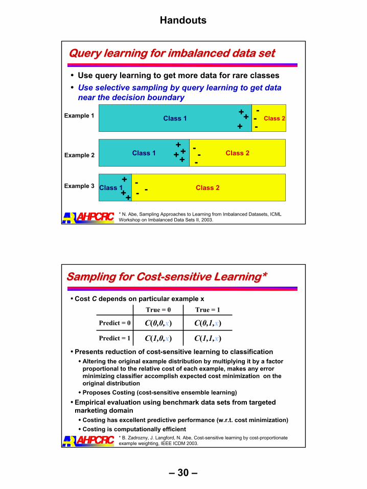
Query learning for imbalanced data set Query learning for imbalanced data set

Use query learning to get more data for rare classesUse selective sampling by query learning to get data near the decision boundary

Class 2Class 1

Class 2Class 1

Class 2Class 1

Example 1

Example 3

+++

++++

+++

--

-

- --

---

Example 2

* N. Abe, Sampling Approaches to Learning from Imbalanced Datasets, ICML Workshop on Imbalanced Data Sets II, 2003.

Sampling for CostSampling for Cost--sensitive Learning*sensitive Learning*

Cost C depends on particular example x

Presents reduction of cost-sensitive learning to classificationAltering the original example distribution by multiplying it by a factor proportional to the relative cost of each example, makes any error minimizing classifier accomplish expected cost minimization on the original distributionProposes Costing (cost-sensitive ensemble learning)

Empirical evaluation using benchmark data sets from targeted marketing domain

Costing has excellent predictive performance (w.r.t. cost minimization) Costing is computationally efficient

* B. Zadrozny, J. Langford, N. Abe, Cost-sensitive learning by cost-proportionate example weighting, IEEE ICDM 2003.

C(1,1,x)C(1,0,x)Predict = 1

C(0,1,x)C(0,0,x)Predict = 0

True = 1True = 0

Handouts

– 31 –

Association Rules for Rare ClassAssociation Rules for Rare Class

Emerging patterns*For 2 classes C1 and C2 and support si(X) of itemset Xin class Ci growth rate is defined as s2(X)/s1(X)Given a threshold p >1, itemset X is p-emerging pattern (EP) if growth rate ≥ pFind EPs in rare classFind values that have the highest growth rate from the major class to the rare classReplace different attribute values in the original rare class EPs with the highest growth rate valuesNew generated EPs have a strong power to discriminate rare class from the major class

* H. Alhammady, K. Rao, The Application of Emerging Patterns for Improving the Quality of Rare-class Classification, PAKDD 2004.

Temporal Analysis of Rare EventsTemporal Analysis of Rare Events

Surprising patterns [Keogh et al, KDD02] A time series pattern P, extracted from database X is surprising relative to a database R, if the probability of its occurrence is greatly different to that expected by chance, assuming that R and X are created by the same underlying process.

Steps (TARZAN algorithm)Discretizing time-series into symbolic strings

Fixed sized sliding windowSlope of the best-fitting line

Calculate probability of any pattern, including ones we have never seen before using Markov modelsFor maintaining linear time and space property, they use suffix tree data structureComputing scores by comparing trees between reference data and incoming information stream

* E. Keogh, et al, Finding Surprising Patterns in a Time Series Database in Linear Time and Space, KDD 2002.

Handouts

– 32 –

Temporal Analysis of Rare EventsTemporal Analysis of Rare Events

Learning to Predict Extremely Rare Events*Genetic-based machine learning system that predicts events by identifying temporal and sequential patterns in data

Temporal Sequence Associations for Rare Events**Predicting Rare Events In Temporal Domains***

Transform event prediction problem into a search for all patterns (event-sets) on the rare class exclusivelyDiscriminative power of patterns is validated against other classesPatterns are then combined into a rule-based model for prediction

* G. Weiss, H. Hirsh, Learning to Predict Extremely Rare Events, AAAI Workshop on Learning from Imbalanced Data Sets, 2000.

** J. Chen, et al, Temporal Sequence Associations for Rare Events, PAKDD 2004

*** R. Vilalta, Predicting Rare Events In Temporal Domains, IEEE ICDM 2002.

Using Clustering for Rare Class Problems*Using Clustering for Rare Class Problems*

Distinguish between regular “between class imbalances”and “within-class imbalance”, where a single class is composed of various sub-classes of different sizeThe procedure

Use clustering to identify subclasses (subclusters)Each subcluster of the majority class is resampled until it reaches the size of the biggest subcluster in the majority class

Denote size of the new majority class as: Size_of_new_majority_class

Each subcluster of the rare class is resampled until it reaches the size

Size_of_majority_class / Nsubclusters_in_rare_class

* N. Japkowicz, Class Imbalances: Are We Focusing on the Right Issues, ICML Workshop on Imbalanced Data Sets II, 2003.

Handouts

– 33 –

Case StudiesCase Studies

Intrusion DetectionNetwork Intrusion DetectionHost based Intrusion Detection

Fraud DetectionCredit Card FraudInsurance Fraud DetectionCell Fraud Detection

Medical DiagnosticsMammogramy imagesHealth Care Fraud

Case Study: Data Mining in Intrusion DetectionCase Study: Data Mining in Intrusion DetectionDue to the proliferation of Internet, more and more organizations are becoming vulnerable to cyber attacksSophistication of cyber attacks as well as their severity is also increasing

Security mechanisms always have inevitable vulnerabilities

Firewalls are not sufficient to ensure security in computer networksInsider attacks

Incidents Reported to Computer Emergency Response Team/Coordination Center (CERT/CC)

Attack sophistication vs. Intruder technical knowledge, source: www.cert.org/archive/ppt/cyberterror.ppt

The geographic spread of Sapphire/Slammer Worm 30 minutes after release (Source: www.caida.org)

0

20000

40000

60000

80000

100000

120000

1 2 3 4 5 6 7 8 9 10 11 12 13 141990 1991 1992 1993 1994 1995 1996 1997 1998 1999 2000 2001 2002 2003

Handouts

– 34 –

What are Intrusions?What are Intrusions?

Intrusions are actions that attempt to bypass security mechanisms of computer systems. They are usually caused by:

Attackers accessing the system from InternetInsider attackers - authorized users attempting to gain and misuse non-authorized privileges

Typical intrusion scenario

Scanning activity

Computer Network

Attacker Machine with vulnerability

What are Intrusions?What are Intrusions?

Intrusions are actions that attempt to bypass security mechanisms of computer systems. They are caused by:

Attackers accessing the system from InternetInsider attackers - authorized users attempting to gain and misuse non-authorized privileges

Typical intrusion scenario

Computer Network

Attacker Compromised Machine

Handouts

– 35 –

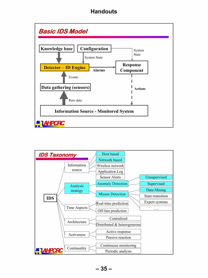
Basic IDS ModelBasic IDS Model

Information Source - Monitored System

Detector – ID Engine Response Component

Data gathering (sensors)

Raw data

Events

Knowledge base Configuration

Alarms

Actions

System State

System State

IDS TaxonomyIDS Taxonomy

IDS

Information source

Analysis strategy

Architecture

Time Aspects

Activeness

Continuality

Host basedNetwork based

Wireless networkApplication Log

Anomaly Detection

Misuse Detection

Unsupervised

SupervisedData Mining

State-transitionExpert systemsReal-time prediction

Off-line prediction

CentralizedDistributed & heterogeneous

Active responsePassive reaction

Continuous monitoringPeriodic analysis

…..

Sensor Alerts

Handouts

– 36 –

IDS IDS -- Analysis StrategyAnalysis Strategy

Misuse detection is based on extensive knowledge of patterns associated with known attacks provided by human experts

Existing approaches: pattern (signature) matching, expert systems, state transition analysis, data miningMajor limitations:

Unable to detect novel & unanticipated attacksSignature database has to be revised for each new type of discovered attack

Anomaly detection is based on profiles that represent normal behavior of users, hosts, or networks, and detecting attacks as significant deviations from this profile

Major benefit - potentially able to recognize unforeseen attacks. Major limitation - possible high false alarm rate, since detected deviations do not necessarily represent actual attacksMajor approaches: statistical methods, expert systems, clustering, neural networks, support vector machines, outlier detection schemes

Intrusion DetectionIntrusion DetectionIntrusion Detection System

combination of software and hardware that attempts to perform intrusion detectionraises the alarm when possible intrusion happens

Traditional intrusion detection system IDS tools (e.g. SNORT) are based on signatures of known attacks

Example of SNORT rule (MS-SQL “Slammer” worm)any -> udp port 1434 (content:"|81 F1 03 01 04 9B 81 F1 01|";content:"sock"; content:"send")

LimitationsSignature database has to be manually revised for each new type of discovered intrusionThey cannot detect emerging cyber threatsSubstantial latency in deployment of newly created signatures across the computer system

Data Mining can alleviate these limitations

www.snort.org

Handouts

– 37 –

Data Mining for Intrusion DetectionData Mining for Intrusion Detection

Increased interest in data mining based intrusion detectionAttacks for which it is difficult to build signaturesAttack stealthinessUnforeseen/Unknown/Emerging attacksDistributed/coordinated attacks

Data mining approaches for intrusion detectionMisuse detection

Building predictive models from labeled labeled data sets (instances are labeled as “normal” or “intrusive”) to identify known intrusionsHigh accuracy in detecting many kinds of known attacksCannot detect unknown and emerging attacks

Anomaly detectionDetect novel attacks as deviations from “normal” behaviorPotential high false alarm rate - previously unseen (yet legitimate) system behaviors may also be recognized as anomalies

Summarization of network traffic

Data Mining Data Mining for Intrusion Detectionfor Intrusion Detection

Misuse Detection –Building Predictive Models

categorical

temporal

continuous

class

TestSet

Training Set Model

Learn Classifier

Tid SrcIP Start time Dest IP Dest

Port Number of bytes Attack

1 206.135.38.95 11:07:20 160.94.179.223 139 192 No

2 206.163.37.95 11:13:56 160.94.179.219 139 195 No

3 206.163.37.95 11:14:29 160.94.179.217 139 180 No

4 206.163.37.95 11:14:30 160.94.179.255 139 199 No

5 206.163.37.95 11:14:32 160.94.179.254 139 19 Yes

6 206.163.37.95 11:14:35 160.94.179.253 139 177 No

7 206.163.37.95 11:14:36 160.94.179.252 139 172 No

8 206.163.37.95 11:14:38 160.94.179.251 139 285 Yes

9 206.163.37.95 11:14:41 160.94.179.250 139 195 No

10 206.163.37.95 11:14:44 160.94.179.249 139 163 Yes 10

Tid SrcIP Start time Dest Port Number

of bytes Attack

1 206.163.37.81 11:17:51 160.94.179.208 150 ?

2 206.163.37.99 11:18:10 160.94.179.235 208 ?

3 206.163.37.55 11:34:35 160.94.179.221 195 ?

4 206.163.37.37 11:41:37 160.94.179.253 199 ?

5 206.163.37.41 11:55:19 160.94.179.244 181 ?

categorical

Anomaly Detection

Rules Discovered:

{Src IP = 206.163.37.95, Dest Port = 139, Bytes ∈ [150, 200]} --> {ATTACK}

Rules Discovered:


Summarization of attacks using association rules

Handouts

– 38 –



categorical

temporal

continuous

class

TestSet

Training Set Model

Learn Classifier



1 206.135.38.95 11:07:20 160.94.179.223 139 192 No

2 206.163.37.95 11:13:56 160.94.179.219 139 195 No

3 206.163.37.95 11:14:29 160.94.179.217 139 180 No

4 206.163.37.95 11:14:30 160.94.179.255 139 199 No

5 206.163.37.95 11:14:32 160.94.179.254 139 19 Yes

6 206.163.37.95 11:14:35 160.94.179.253 139 177 No

7 206.163.37.95 11:14:36 160.94.179.252 139 172 No

8 206.163.37.95 11:14:38 160.94.179.251 139 285 Yes

9 206.163.37.95 11:14:41 160.94.179.250 139 195 No

10 206.163.37.95 11:14:44 160.94.179.249 139 163 Yes 10

Tid SrcIP Start time Dest IP Number

of bytes Attack

1 206.163.37.81 11:17:51 160.94.179.208 150 No

2 206.163.37.99 11:18:10 160.94.179.235 208 No

3 206.163.37.55 11:34:35 160.94.179.221 195 Yes

4 206.163.37.37 11:41:37 160.94.179.253 199 No

5 206.163.37.41 11:55:19 160.94.179.244 181 Yes

categorical

Anomaly Detection

Rules Discovered:


Rules Discovered:





categorical

temporal

continuous

class

TestSet

Training Set Model

Learn Classifier



1 206.135.38.95 11:07:20 160.94.179.223 139 192 No

2 206.163.37.95 11:13:56 160.94.179.219 139 195 No

3 206.163.37.95 11:14:29 160.94.179.217 139 180 No

4 206.163.37.95 11:14:30 160.94.179.255 139 199 No

5 206.163.37.95 11:14:32 160.94.179.254 139 19 Yes

6 206.163.37.95 11:14:35 160.94.179.253 139 177 No

7 206.163.37.95 11:14:36 160.94.179.252 139 172 No

8 206.163.37.95 11:14:38 160.94.179.251 139 285 Yes

9 206.163.37.95 11:14:41 160.94.179.250 139 195 No

10 206.163.37.95 11:14:44 160.94.179.249 139 163 Yes 10

categorical

Anomaly Detection

Rules Discovered:


Rules Discovered:



Tid SrcIP Start time Dest IP Number

of bytes Attack

1 206.163.37.81 11:17:51 160.94.179.208 150 No

2 206.163.37.99 11:18:10 160.94.179.235 208 No

3 206.163.37.55 11:34:35 160.94.179.221 195 Yes

4 206.163.37.37 11:41:37 160.94.179.253 199 No

5 206.163.37.41 11:55:19 160.94.179.244 181 Yes

Handouts

– 39 –

Data Preprocessing for Data Mining in IDData Preprocessing for Data Mining in ID

Converting the data from monitored system (computer network, host machine, …) into data (features) that will be used in data mining models

For misuse detection, labeling data examples into normal or intrusive may require enormous time for many human experts

Building data mining modelsMisuse detection modelsAnomaly detection models

Analysis and summarization of results

Feature construction

Building data mining models

features

Analysis of results

Data Sources in Network Intrusion DetectionData Sources in Network Intrusion Detection

Network traffic data is usually collected using “network sniffers”Tcpdump

08:02:15.471817 0:10:7b:38:46:33 0:10:7b:38:46:33 loopback 60: 0000 0100 0000 0000 0000 0000 0000 00000000 0000 0000 0000 0000 0000 0000 00000000 0000 0000 0000 0000 0000 0000

08:02:19.391039 172.16.112.100.3055 > 172.16.112.10.ntp: v1 client strat 0 poll 0 prec 008:02:19.391456 172.16.112.10.ntp > 172.16.112.100.3055: v1 server strat 5 poll 4 prec -16 (DF)

net-flow toolsSource and destination IP address, Source and destination ports, Type of service, Packet and byte counts, Start and end time, Input and output interface numbers, TCP flags, Routing information (next-hop address, source autonomous system (AS) number, destination AS number)

0624.12:4:39.344 0624.12:4:48.292 211.59.18.101 4350 160.94.179.138 1433 6 2 3 1440624.9:1:10.667 0624.9:1:19.635 24.201.13.122 3535 160.94.179.151 1433 6 2 3 1320624.12:4:40.572 0624.12:4:49.496 211.59.18.101 4362 160.94.179.150 1433 6 2 3 152

Collected data are in the form of network connections or networkpackets (a network connection may contain several packets)

Handouts

– 40 –

Feature Construction in Intrusion DetectionFeature Construction in Intrusion Detection

Basic set of features (start/end time, srcIP, dstIP, srcport, dstport, protocol, TCP flags, # of bytes, packets, …)Three groups of features may be constructed (KDDCup 99):

“content-based” features within a connection Intrinsic characteristics of data packetsnumber of failed logins, root logins, acknowledgments, directory creations, …)

time-based traffic features included number of connections or different services from the same source or to the same destination considering recent time interval (e.g.a few seconds)

Useful for detecting scanning activities

connection based features included number of connections from same source or to same destination or with the same service considering in last N connections

Useful for detecting SLOW scanning activities

MADAM ID MADAM ID -- Feature Construction ExampleFeature Construction Example

Example: “syn flood” patterns (service=http, flag=SYN, victim), (service=http, flag=SYN, victim) → (service = http, SYN, victim) [0.9, 0.02, 2s]

After 2 http packets with set SYN flag are sent to victim, in 90% of cases third connection is made within 2s. This happens in 2% of all connections (support = 2%)Add features based on frequent episodes learned separately for normal data and attack data

count the connections in the past 2 secondscount the connections with the same characteristics (http, SYN, victim) in the past 2 seconds

Different features are found for different classes of attacks =>different models for the classes

flagdst … service …h1 http S0h1 http S0h1 http S0

h2 http S0

h4 http S0

h2 ftp S0

syn flood

normal

existing features existing features uselessuseless


h2 http S0

h4 http S0

h2 ftp S0

syn flood

normal


h2 http S0

h4 http S0

h2 ftp S0

syn flood

normal

existing features existing features uselessuseless

dst … service …h1 http S0h1 http S0h1 http S0

h2 http S0

h4 http S0

h2 ftp S0

flag %S0707275

0

0

0

construct features with construct features with high information gainhigh information gain


h2 http S0

h4 http S0

h2 ftp S0

flag %S0707275

0

0

0


h2 http S0

h4 http S0

h2 ftp S0

flag %S0707275

0

0

0

construct features with construct features with high information gainhigh information gain

Handouts

– 41 –

MADAM ID Workflow*MADAM ID Workflow*

Association rules and frequent episodes are applied to network connection records to obtain additional features for data mining algorithmsApply RIPPER to labeled data sets and learn the intrusions

Raw audit data

network packets/events

Connection records

RIPPER Model

patterns features

Feature constructor Evaluation feedback

* W. Lee,S. Stolfo, Adaptive Intrusion Detection: a Data Mining Approach, Artificial Intelligence Review, 2000

MADAM ID MADAM ID -- CostCost--sensitive Modelingsensitive Modeling

A multiple-model approach:Certain features are more costly to compute than othersBuild multiple rule-sets, each with features of different cost levelsCost factors: damage cost, response cost, operational cost (level 1-4 features)

Level 1: beginning of an eventLevel 2: middle to end of an eventLevel 3: at the end of an eventLevel 4: at the end of an event, multiple events in a time window

Use cheaper rule-sets first, costlier ones later only for required accuracy

* W. Lee,et al., Toward Cost-Sensitive Modeling for Intrusion Detection and Response, Journal of Computer Security, 2002

Handouts

– 42 –

ADAM*ADAM*

Data mining testbed that uses combination of association rules and classification to discover attacksI phase: ADAM builds a repository of profiles for “normal frequent itemsets” by mining “attack-free” dataII phase: ADAM runs a sliding window, incremental algorithm that finds frequent itemsets in the last N connections and compare them to “normal” profile

Tunable: different thresholds can be set for different types of rules.Anomaly detection: first characterize normal behavior (profile), then flag abnormal behaviorReduced false alarm rate: using a classifier.

* D. Barbara, et al., ADAM: A Testbed for Exploring the Use of Data Mining in Intrusion Detection. SIGMOD Record 2001.

Attack-free data

ADAM: Training phaseADAM: Training phase

Database of frequent itemsets for attack-free data is madeFor entire training data, find suspicious frequent itemsetsthat are not in the “attack-free” databaseTrain a classifier to classify itemset as known attack, unknown attack or normal event

Data preprocessing

tcpdumpdata

Training data

Classifier

Handouts

– 43 –

ADAM: Phase of Discovering IntrusionsADAM: Phase of Discovering Intrusions

Dynamic mining module produces suspicious itemsetsfrom test dataAlong with features from feature selection module, itemsets are fed to classifier

Feature selection

Test data Dynamic mining

profile

Classifier

Attacks, False alarms, Unknown

Data preprocessing

tcpdumpdata

The MINDS Project*The MINDS Project*

MINDS – Minnesota Intrusion Detection SystemMINDS

network

Data capturing device

Anomaly detection

……

Anomaly scores

Humananalyst

Detected novel attacks

Summary and characterization

of attacks

MINDS system

Known attack detection

Detected known attacks

Labels

Feature Extraction

Association pattern analysis

MINDSAT

Filtering

Net flow tools

tcpdump

MINDS has been incorporated into the Interrogator architecture at the Army Research Labs (ARL) Center for Intrusion Monitoring and Protection (CIMP), where network data from multiple sensors is collected and analyzed.The MINDS is being used at University of Minnesota and at the ARL-CIMP to help analysts to detect attacks and intrusive behavior that cannot be detected using widely used intrusion detection systems, such as SNORT.

* - Ertoz, L., Eilertson, E., Lazarevic, et al, The MINDS - Minnesota Intrusion Detection System, review for the book “Data Mining: Next Generation Challenges and Future Directions”, AAAI/MIT Press.

Handouts

– 44 –

Alternative Classification ApproachesAlternative Classification Approaches

Fuzzy Data Mining in network intrusion detection (MSU)*Create fuzzy association rules only from normal data to learn “normal behavior”

For new audit data, create the set of fuzzy association rules and compute its similarity to the “normal” oneIf similarity low ⇒ for new data generate alarm

Genetic algorithms (GA) used to tune membership function of the fuzzy sets

Fitness – rewards for high similarity between normal and reference data, penalizing – high similarity between intrusion and reference data

Use GA to select most relevant features

* S. Bridges, R. Vaughn, Intrusion Detection Via Fuzzy Data Mining, 2000

Alternative Classification Approaches*Alternative Classification Approaches*

Scalable Clustering Technique*Apply supervised clustering

For each point find nearest point and if belong to the same class, append to the same cluster, else create a new

ClassificationClass dominated in k nearest clustersWeighted sum of distances to k nearest clusters

Incremental clustering

Distances: weighted Euclidean, Chi-square, Canbera

(d(x, L)) =

* N. Ye, X. Li, A Scalable Clustering for Intrusion Signature Recognition, 2001.

∑= +

−d

ii

ii

ii CLxLx

1

2|| Li – i-th attribute of centroid of the cluster L

Ci – correlation between i-th attribute and the class

Handouts

– 45 –

Neural Networks Classification ApproachesNeural Networks Classification Approaches

Neural networks (NNs) applied to host-based intrusion detection

Building profiles of users according to used commands Building profiles of software behavior

Neural networks for network-based intrusion detection

Hierarchical network intrusion detectionMulti-layer perceptrons (MLP)*Self organizing maps (SOMs)*

* J. Canady, J. Mahaffey, The Application of Artificial Neural Networks to Misuse Detection:Initial Results, 1998.


Packet level (PHAD) and Application level (ALAD) anomaly detectiPacket level (PHAD) and Application level (ALAD) anomaly detection*on*PHAD (packet header anomaly detection) monitors Ethernet, IP andtransport layer packet headers

It builds profiles for 33 different fields from these headers by looking attack free traffic and performs clustering (prespecifed # of clusters)A new value that does not fit into any of the clusters (intervals), it is treated as a new cluster and closest two clusters are mergedThe number of updates, r, is maintained for each field as well as the number of observations, nTesting: For each new observed packet, if the value for some attribute does not fit into the clusters, anomaly score for that attribute is proportional to n/r

ALAD uses the same method for anomaly scores, but it works only on TCP data and build TCP streams

It build profiles for 5 different features

* M. Mahoney, P. Chan: Learning Nonstationary Models of Normal Network Traffic for Detecting Novel Attacks, 8th ACM KDD, 2002

Handouts

– 46 –

NATE*NATE*

Low-cost anomaly detection algorithmIt uses only header information5 features are used:

Counts of Push and Ack TCP flags (Syn, Fin, Reset and Urgent TCP flags are dropped due to their small variability)Total number of packets Number of bytes transferred for each packet (bytes / packet) Percent of control packets per session

Builds clusters for normal behaviorMultivariate normal distribution to model clustersFor each test point compute Mahalanobis distance to every cluster

* C. Taylor and J. Alves-Foss. NATE - Network Analysis of Anomalous Traffic Events, A Low-Cost Approach, Proc. New Security Paradigms Workshop. 2001.

Summarization of Anomalous Connections*Summarization of Anomalous Connections*

MINDS example: January 26, 2003 (48 hours after the Slammer worm)score srcIP sPort dstIP dPort protocoflags packets bytes37674.69 63.150.X.253 1161 128.101.X.29 1434 17 16 [0,2) [0,1829)26676.62 63.150.X.253 1161 160.94.X.134 1434 17 16 [0,2) [0,1829)24323.55 63.150.X.253 1161 128.101.X.185 1434 17 16 [0,2) [0,1829)21169.49 63.150.X.253 1161 160.94.X.71 1434 17 16 [0,2) [0,1829)19525.31 63.150.X.253 1161 160.94.X.19 1434 17 16 [0,2) [0,1829)19235.39 63.150.X.253 1161 160.94.X.80 1434 17 16 [0,2) [0,1829)17679.1 63.150.X.253 1161 160.94.X.220 1434 17 16 [0,2) [0,1829)8183.58 63.150.X.253 1161 128.101.X.108 1434 17 16 [0,2) [0,1829)7142.98 63.150.X.253 1161 128.101.X.223 1434 17 16 [0,2) [0,1829)5139.01 63.150.X.253 1161 128.101.X.142 1434 17 16 [0,2) [0,1829)4048.49 142.150.Y.101 0 128.101.X.127 2048 1 16 [2,4) [0,1829)4008.35 200.250.Z.20 27016 128.101.X.116 4629 17 16 [2,4) [0,1829)3657.23 202.175.Z.237 27016 128.101.X.116 4148 17 16 [2,4) [0,1829)3450.9 63.150.X.253 1161 128.101.X.62 1434 17 16 [0,2) [0,1829)3327.98 63.150.X.253 1161 160.94.X.223 1434 17 16 [0,2) [0,1829)2796.13 63.150.X.253 1161 128.101.X.241 1434 17 16 [0,2) [0,1829)2693.88 142.150.Y.101 0 128.101.X.168 2048 1 16 [2,4) [0,1829)2683.05 63.150.X.253 1161 160.94.X.43 1434 17 16 [0,2) [0,1829)2444.16 142.150.Y.236 0 128.101.X.240 2048 1 16 [2,4) [0,1829)2385.42 142.150.Y.101 0 128.101.X.45 2048 1 16 [0,2) [0,1829)2114.41 63.150.X.253 1161 160.94.X.183 1434 17 16 [0,2) [0,1829)2057.15 142.150.Y.101 0 128.101.X.161 2048 1 16 [0,2) [0,1829)1919.54 142.150.Y.101 0 128.101.X.99 2048 1 16 [2,4) [0,1829)1634.38 142.150.Y.101 0 128.101.X.219 2048 1 16 [2,4) [0,1829)1596.26 63.150.X.253 1161 128.101.X.160 1434 17 16 [0,2) [0,1829)1513.96 142.150.Y.107 0 128.101.X.2 2048 1 16 [0,2) [0,1829)1389.09 63.150.X.253 1161 128.101.X.30 1434 17 16 [0,2) [0,1829)1315.88 63.150.X.253 1161 128.101.X.40 1434 17 16 [0,2) [0,1829)1279.75 142.150.Y.103 0 128.101.X.202 2048 1 16 [0,2) [0,1829)1237.97 63.150.X.253 1161 160.94.X.32 1434 17 16 [0,2) [0,1829)1180.82 63.150.X.253 1161 128.101.X.61 1434 17 16 [0,2) [0,1829)1107.78 63.150.X.253 1161 160.94.X.154 1434 17 16 [0,2) [0,1829)

Potential Rules:1.

{Dest Port = 1434/UDP #packets ∈ [0, 2)} --> Highly anomalous behavior (Slammer Worm)

2.

{Src IP = 142.150.Y.101, Dest Port = 2048/ICMP #bytes ∈ [0, 1829]} --> Highly anomalous behavior (ping – scan)

Potential Rules:1.

{Dest Port = 1434/UDP #packets ∈ [0, 2)} --> Highly anomalous behavior (Slammer Worm)

2.

{Src IP = 142.150.Y.101, Dest Port = 2048/ICMP #bytes ∈ [0, 1829]} --> Highly anomalous behavior (ping – scan)

* - Ertoz, L., Eilertson, E., Lazarevic, et al, The MINDS - Minnesota Intrusion Detection System, review for the book “Data Mining: Next Generation Challenges and Future Directions”, AAAI/MIT Press.

Handouts

– 47 –

Profiling based anomaly detectionProfiling based anomaly detection

Profiling methods are usually applied to host based intrusion detection where users, programs, etc. are profiled

Profiling sequences of Unix shell command lines*Set of sequences (user profiles) reduced and filtered to reduce data set for analysisBuild Instance Based Learning (IBL) model that stores historic examples of “normal” data

Compares new data stream Distance measure that favors long temporal similar sequencesEvent sequences are segmented

Profiling users’ behaviorUsing neural networks

a b c d a g c e

a b c d g b c d

* T. Lane, C. Brodley, Temporal Sequence Learning and Data Reduction for Anomaly detection, 1998.

Case Study: Data Mining in Fraud DetectionCase Study: Data Mining in Fraud Detection

Fraud detection in E-commerce/ business worldCredit Card Fraud

Internet Transaction Fraud / E-Cash fraud

Insurance Fraud and Health Care Fraud

Money Laundering

Telecommunications Fraud

Subscription Fraud / Identity Theft

All major data miming techniques applicable to intrusion detection are also applicable to fraud detection domains mentioned above

Handouts

– 48 –

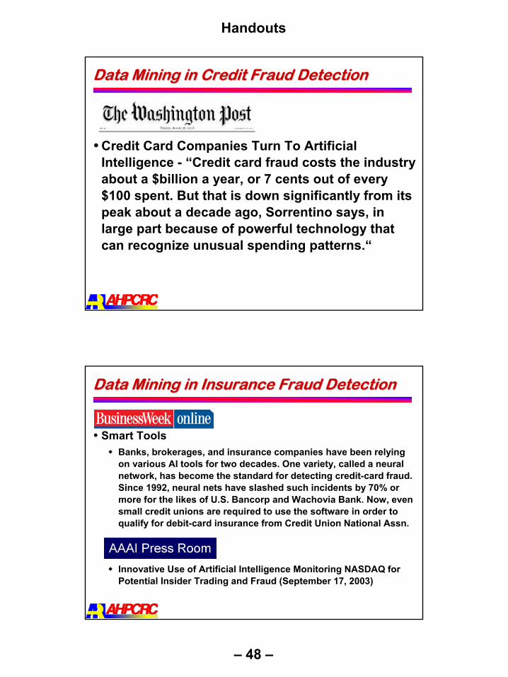
Data Mining in Credit Fraud DetectionData Mining in Credit Fraud Detection

Credit Card Companies Turn To Artificial Intelligence - “Credit card fraud costs the industry about a $billion a year, or 7 cents out of every $100 spent. But that is down significantly from its peak about a decade ago, Sorrentino says, in large part because of powerful technology that can recognize unusual spending patterns.“

Data Mining in Insurance Fraud DetectionData Mining in Insurance Fraud Detection

Smart Tools Banks, brokerages, and insurance companies have been relying on various AI tools for two decades. One variety, called a neural network, has become the standard for detecting credit-card fraud. Since 1992, neural nets have slashed such incidents by 70% or more for the likes of U.S. Bancorp and Wachovia Bank. Now, even small credit unions are required to use the software in order toqualify for debit-card insurance from Credit Union National Assn.

Innovative Use of Artificial Intelligence Monitoring NASDAQ for Potential Insider Trading and Fraud (September 17, 2003)

Handouts

– 49 –

Data Mining in Cell Fraud DetectionData Mining in Cell Fraud Detection

Phone Friend - "More than 15,000 mobile phones are stolen each month in Britain alone. According to Swedish cellphone maker Ericsson, the fraudulent use of stolen mobiles means a loss of between two and five per cent of revenue for the network operators.“

Ericsson Enlists AI To Fight Wireless FraudMobile network operators claim that 2 to 5 percent of total revenues are lost to fraud, and the problem is expected to worsen

Data Mining Techniques in Fraud DetectionData Mining Techniques in Fraud Detection

Basic approachesJAM project [Chan99]Neural networks [Brauser99, Maes00, Dorronsoro97]Adaptive fraud detection [Fawcett97]Account signatures [Cahill02]Statistical Fraud Detection [Bolton 2002]Fraud detection in mobile telecommunication networks [Burge96]User profiling and classification for fraud detection in mobile telecommunication networks [Hollmen00]

Handouts

– 50 –

JAM Project*JAM Project*

JAVA agents for meta-learningLaunch learning agents to remote data sitesExchange remote classifiersLocal meta-learning agentsproduce meta-classifierLaunch meta-classifier to remote data sites

Chase credit card (20% fraud), First Union credit card (15% fraud) – 500,000 data records5 base classifiers (Bayes, C4.5, CART, ID3, RIPPER)Select the classifier with the highest TP-FP rate on the validation set

* JAM Project, http://www1.cs.columbia.edu/~sal/JAM/PROJECT/

JAM Project JAM Project -- ExampleExample

TP-FP rate vs. the number of classifiers

• Input base classifiers:First Union

• Test data set:First Union

• Best meta classifier:Naïve Bayes with 10-17 base classifiers.

Handouts

– 51 –

Neural Networks in Fraud Detection*Neural Networks in Fraud Detection*

Use an expert net for each feature group (e.g. time,money) and group the experts together to form a common vote*

Standard application of neural networks in credit card fraud detection **Use a non-linear version of Fisher’sdiscriminant analysis, which separates a good proportion of fraudulent operations away from other closer to normal traffic

* R. Brause,T. Langsdorf, M. Hepp, Neural Data Mining for Credit Card Fraud Detection, 11th IEEE International Conference on Tools with Artificial Intelligence, 1999.

** S. Maes, et al, Credit Card Fraud Detection Using Bayesian and Neural Networks, NAISO Congress on NEURO FUZZY THECHNOLOGIES, 2002

*** J. Dorronsoro, F. Ginel, C. Sánchez, C. Santa Cruz, Neural Fraud Detection in Credit Card Operations, IEEE Trans. Neural Networks, 8 (1997), pp. 827-834

Fraud Detection in Telecommunication NetworksFraud Detection in Telecommunication Networks

Identify relevant user groups based on call data and then assign a user to a relevant group

call data is subsequently used in describing behavioral patterns of users

Neural networks and probabilistic models are employed in learning these usage patterns from call dataThese models are used either to detect abrupt changes in established usage patterns or to recognize typical usage patterns of fraud

• J. Hollmen, User profiling and classification for fraud detection in mobile communications networks, PhD thesis, Helsinki University of Technology, 2000.

• P. Burge, J. Shawe-Taylor, Frameworks for Fraud Detection in mobile communications networks, 1996.

Handouts

– 52 –

Case Study: Medical DiagnosisCase Study: Medical Diagnosis

Cost of false positive error: Unnecessary treatment; unnecessary worryCost of false negative error: Postponed treatment or failure to treat; death or injuryEvent Rate Reference Bleeding in outpatients on warfarin 6.7%/yr Beyth 1998

Medication errors per order 5.3% (n=10070) Bates 1995

Medication error per order 0.3% (n=289000) Lesar 1997

Adverse drug events per admission 6.5% Bates 1995

Adverse drug events per order 0.05% (n=10070) Bates 1995

Adverse drug events per patient 6.7% Lazarou 1998

Adverse drug events per patient 1.2% Bains 1999

Adverse drug events in nursing home patients 1.89/100 pt-months Gurwitz Nosocomial infections in older hospitalized patients 5.9 to 16.9 per 1000 days Rothchild 2000

Pressure ulcers 5% Rothschild 2000

Data Mining in Medical DiagnosisData Mining in Medical Diagnosis

Introducing noise to rare class examples*For each attribute i, noisy example = xi + εi, where , Σq is qxq diagonal matrix diag{s1

2, …, sq2}, si

2 – sample variance of xi

Hierarchical neural nets (HNNs)**HNNs are designed according to a divide-and-conquer approach

Triage networks are able to discriminate supersets that contain the infrequent patternThese supersets are then used by specialized networks

),,0( 2qnoisei N Σ≈ σε

* S. Lee, Noisy replication in skewed binary classification, Computational Statistics & Data Analysis August, 2000.

** L.Machado, Identification of Low Frequency Patterns in Backpropagation Neural Networks, Annual Symposium on Computer Applications in Medical Care, 1994.

Handouts

– 53 –

Data Mining in Medical DiagnosisData Mining in Medical Diagnosis

Spectrum and response analysis for neural nets*Data: polyproline type II (PPII) secondary structure

PPII structure is rare (1.26%)Around an individual case (sequence) there is a hyper-sphere with a high probability area for the same secondary structure type

Sample stratification schemes for neural networks (NNs)**1. stratifies a sample by adding up the weighted sum of the

derivatives during the backward pass of training2. After training NNs with multiple sets of bootstrapped examples of

the rare event classes and subsampled examples of common event classes, multiple voting for classification is performed

* M. Siermala, Local Prediction of Secondary Structures of Proteins from Viewpoints of Rare Structure, PhD Thesis, University of Tampere, May 2002.

** W. Choe et al, Neural network schemes for detecting rare events in human genomic DNA, Bioinformatics. 2000.

ConclusionsConclusions

Data mining analysis of rare events requires special attentionMany real world applications exhibit “needle-in-the-haystack” type of problem Current “state of the art” data mining techniques are still insufficient for efficient handling rare eventsNeed for designing better and more accurate data mining models

Handouts

– 54 –

LinksLinks

Intrusion Detection bibliographywww.cs.umn.edu/~aleks/intrusion_detection.htmlwww.cs.fit.edu/~pkc/id/related/index.htmlwww.cc.gatech.edu/~wenke/ids-readings.htmlwww.cerias.purdue.edu/coast/intrusion-detection/welcome.htmlhttp://cnscenter.future.co.kr/security/ids.htmlwww.cs.purdue.edu/homes/clifton/cs590m/www.cs.ucsb.edu/~rsg/STAT/links.html

Fraud detection bibliographywww.hpl.hp.com/personal/Tom_Fawcett/fraud-public.bib.gzhttp://dinkla.net !!!!!http://www.aaai.org/AITopics/html/fraud.html

Fraud detection solutionswww.kdnuggets.com/solutions/fraud-detection.html

Questions?Questions?

Thank You!

Contact: [email protected]

[email protected]

[email protected]

data mining for analysis of rare events: a case study in ...aleks/pakdd04_tutorial.pdfdata mining...

Documents