data mining classification: alternative...
TRANSCRIPT

Data Mining Classification: Alternative Techniques
Lecture Notes for Chapter 5
Introduction to Data Mining
by
Tan, Steinbach, Kumar
© Tan,Steinbach, Kumar Introduction to Data Mining 4/18/2004 1

© Tan,Steinbach, Kumar Introduction to Data Mining 4/18/2004 ‹#›
Rule-Based Classifier
� Classify records by using a collection of “if…then…” rules
� Rule: (Condition) → y
– where
� Condition is a conjunctions of attributes
� y is the class label
– LHS: rule antecedent or condition
– RHS: rule consequent
– Examples of classification rules:
� (Blood Type=Warm) ∧ (Lay Eggs=Yes) → Birds
� (Taxable Income < 50K) ∧ (Refund=Yes) → Evade=No

© Tan,Steinbach, Kumar Introduction to Data Mining 4/18/2004 ‹#›
Rule-based Classifier (Example)
R1: (Give Birth = no) ∧ (Can Fly = yes) → Birds
R2: (Give Birth = no) ∧ (Live in Water = yes) → Fishes
R3: (Give Birth = yes) ∧ (Blood Type = warm) → Mammals
R4: (Give Birth = no) ∧ (Can Fly = no) → Reptiles
R5: (Live in Water = sometimes) → Amphibians
Name Blood Type Give Birth Can Fly Live in Water Class
human warm yes no no mammalspython cold no no no reptilessalmon cold no no yes fisheswhale warm yes no yes mammalsfrog cold no no sometimes amphibianskomodo cold no no no reptilesbat warm yes yes no mammalspigeon warm no yes no birdscat warm yes no no mammalsleopard shark cold yes no yes fishesturtle cold no no sometimes reptilespenguin warm no no sometimes birdsporcupine warm yes no no mammalseel cold no no yes fishessalamander cold no no sometimes amphibiansgila monster cold no no no reptilesplatypus warm no no no mammalsowl warm no yes no birdsdolphin warm yes no yes mammalseagle warm no yes no birds

© Tan,Steinbach, Kumar Introduction to Data Mining 4/18/2004 ‹#›
Application of Rule-Based Classifier
� A rule r covers an instance x if the attributes of the instance satisfy the condition of the rule
R1: (Give Birth = no) ∧ (Can Fly = yes) → Birds
R2: (Give Birth = no) ∧ (Live in Water = yes) → Fishes
R3: (Give Birth = yes) ∧ (Blood Type = warm) → Mammals
R4: (Give Birth = no) ∧ (Can Fly = no) → Reptiles
R5: (Live in Water = sometimes) → Amphibians
The rule R1 covers a hawk => Bird
The rule R3 covers the grizzly bear => Mammal
Name Blood Type Give Birth Can Fly Live in Water Class
hawk warm no yes no ?grizzly bear warm yes no no ?

© Tan,Steinbach, Kumar Introduction to Data Mining 4/18/2004 ‹#›
Rule Coverage and Accuracy
� Coverage of a rule:
– Fraction of records that satisfy the antecedent of a rule
� Accuracy of a rule:
– Fraction of records that satisfy both the antecedent and consequent of a rule
Tid Refund Marital Status
Taxable Income Class
1 Yes Single 125K No
2 No Married 100K No
3 No Single 70K No
4 Yes Married 120K No
5 No Divorced 95K Yes
6 No Married 60K No
7 Yes Divorced 220K No
8 No Single 85K Yes
9 No Married 75K No
10 No Single 90K Yes 10
(Status=Single) →→→→ No
Coverage = 40%, Accuracy = 50%
© Tan,Steinbach, Kumar Introduction to Data Mining 4/18/2004 ‹#›
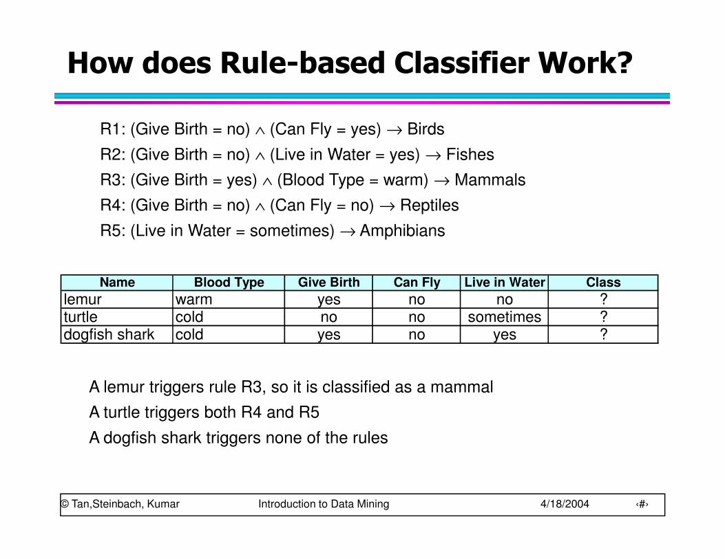
How does Rule-based Classifier Work?
R1: (Give Birth = no) ∧ (Can Fly = yes) → Birds
R2: (Give Birth = no) ∧ (Live in Water = yes) → Fishes
R3: (Give Birth = yes) ∧ (Blood Type = warm) → Mammals
R4: (Give Birth = no) ∧ (Can Fly = no) → Reptiles
R5: (Live in Water = sometimes) → Amphibians
A lemur triggers rule R3, so it is classified as a mammal
A turtle triggers both R4 and R5
A dogfish shark triggers none of the rules
Name Blood Type Give Birth Can Fly Live in Water Class
lemur warm yes no no ?turtle cold no no sometimes ?dogfish shark cold yes no yes ?
© Tan,Steinbach, Kumar Introduction to Data Mining 4/18/2004 ‹#›
Characteristics of Rule-Based Classifier
� Mutually exclusive rules
– Classifier contains mutually exclusive rules if the rules are independent of each other
– Every record is covered by at most one rule
� Exhaustive rules
– Classifier has exhaustive coverage if it accounts for every possible combination of attribute values
– Each record is covered by at least one rule

© Tan,Steinbach, Kumar Introduction to Data Mining 4/18/2004 ‹#›
From Decision Trees To Rules
YESYESNONO
NONO
NONO
Yes No
{Married}{Single,
Divorced}
< 80K > 80K
Taxable
Income
Marital
Status
Refund
Classification Rules
(Refund=Yes) ==> No
(Refund=No, Marital Status={Single,Divorced},Taxable Income<80K) ==> No
(Refund=No, Marital Status={Single,Divorced},Taxable Income>80K) ==> Yes
(Refund=No, Marital Status={Married}) ==> No
Rules are mutually exclusive and exhaustive
Rule set contains as much information as the tree

© Tan,Steinbach, Kumar Introduction to Data Mining 4/18/2004 ‹#›
Rules Can Be Simplified
YESYESNONO
NONO
NONO
Yes No
{Married}{Single,
Divorced}
< 80K > 80K
Taxable
Income
Marital
Status
Refund
Tid Refund Marital Status
Taxable Income Cheat
1 Yes Single 125K No
2 No Married 100K No
3 No Single 70K No
4 Yes Married 120K No
5 No Divorced 95K Yes
6 No Married 60K No
7 Yes Divorced 220K No
8 No Single 85K Yes
9 No Married 75K No
10 No Single 90K Yes 10
Initial Rule: (Refund=No) ∧ (Status=Married) →→→→ No
Simplified Rule: (Status=Married) →→→→ No
© Tan,Steinbach, Kumar Introduction to Data Mining 4/18/2004 ‹#›
Effect of Rule Simplification
� Rules are no longer mutually exclusive
– A record may trigger more than one rule
– Solution?
� Ordered rule set
� Unordered rule set – use voting schemes
� Rules are no longer exhaustive
– A record may not trigger any rules
– Solution?
� Use a default class

© Tan,Steinbach, Kumar Introduction to Data Mining 4/18/2004 ‹#›
Ordered Rule Set
� Rules are rank ordered according to their priority– An ordered rule set is known as a decision list
� When a test record is presented to the classifier – It is assigned to the class label of the highest ranked rule it has
triggered
– If none of the rules fired, it is assigned to the default class
R1: (Give Birth = no) ∧ (Can Fly = yes) → Birds
R2: (Give Birth = no) ∧ (Live in Water = yes) → Fishes
R3: (Give Birth = yes) ∧ (Blood Type = warm) → Mammals
R4: (Give Birth = no) ∧ (Can Fly = no) → Reptiles
R5: (Live in Water = sometimes) → Amphibians
Name Blood Type Give Birth Can Fly Live in Water Class
turtle cold no no sometimes ?

© Tan,Steinbach, Kumar Introduction to Data Mining 4/18/2004 ‹#›
Rule Ordering Schemes
� Rule-based ordering– Individual rules are ranked based on their quality
� Class-based ordering– Rules that belong to the same class appear together

© Tan,Steinbach, Kumar Introduction to Data Mining 4/18/2004 ‹#›
Building Classification Rules
� Direct Method:
� Extract rules directly from data
� e.g.: RIPPER, CN2, Holte’s 1R
� Indirect Method:
� Extract rules from other classification models (e.g. decision trees, neural networks, etc).
� e.g: C4.5rules

© Tan,Steinbach, Kumar Introduction to Data Mining 4/18/2004 ‹#›
Direct Method: Sequential Covering
1. Start from an empty rule
2. Grow a rule using the Learn-One-Rule function
3. Remove training records covered by the rule
4. Repeat Step (2) and (3) until stopping criterion is met

© Tan,Steinbach, Kumar Introduction to Data Mining 4/18/2004 ‹#›
Example of Sequential Covering
(ii) Step 1

© Tan,Steinbach, Kumar Introduction to Data Mining 4/18/2004 ‹#›
Example of Sequential Covering…
(iii) Step 2
R1
(iv) Step 3
R1
R2

© Tan,Steinbach, Kumar Introduction to Data Mining 4/18/2004 ‹#›
Aspects of Sequential Covering
� Rule Growing
� Instance Elimination
� Rule Evaluation
� Stopping Criterion
� Rule Pruning

© Tan,Steinbach, Kumar Introduction to Data Mining 4/18/2004 ‹#›
Rule Growing
� Two common strategies

© Tan,Steinbach, Kumar Introduction to Data Mining 4/18/2004 ‹#›
Rule Growing (Examples)
� CN2 Algorithm:– Start from an empty conjunct: {}
– Add conjuncts that minimizes the entropy measure: {A}, {A,B}, …
– Determine the rule consequent by taking majority class of instances covered by the rule
� RIPPER Algorithm:– Start from an empty rule: {} => class
– Add conjuncts that maximizes FOIL’s information gain measure:
� R0: {} => class (initial rule)
� R1: {A} => class (rule after adding conjunct)
� Gain(R0, R1) = t [ log (p1/(p1+n1)) – log (p0/(p0 + n0)) ]
� where t: number of positive instances covered by both R0 and R1
p0: number of positive instances covered by R0
n0: number of negative instances covered by R0
p1: number of positive instances covered by R1
n1: number of negative instances covered by R1

© Tan,Steinbach, Kumar Introduction to Data Mining 4/18/2004 ‹#›
Instance Elimination
� Why do we need to eliminate instances?
– Otherwise, the next rule is identical to previous rule
� Why do we remove positive instances?
– Ensure that the next rule is different
� Why do we remove negative instances?
– Prevent underestimating accuracy of rule
– Compare rules R2 and R3 in the diagram
© Tan,Steinbach, Kumar Introduction to Data Mining 4/18/2004 ‹#›
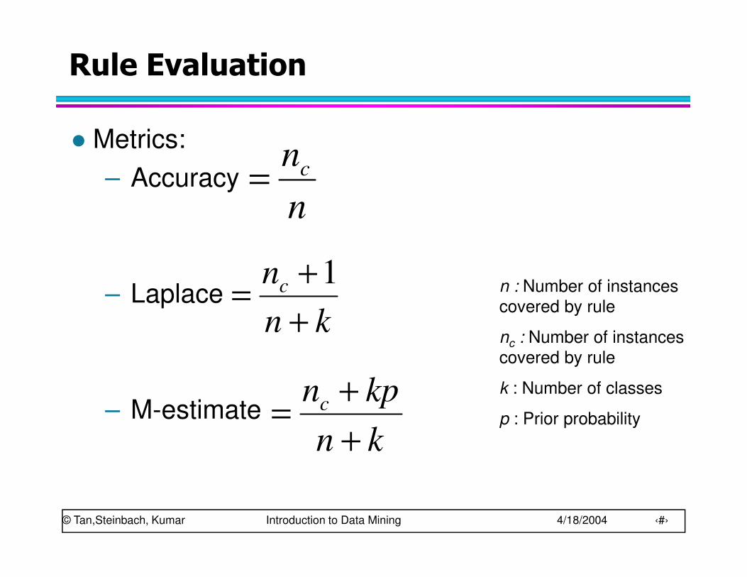
Rule Evaluation
� Metrics:
– Accuracy
– Laplace
– M-estimate
kn
nc
+
+=
1
kn
kpnc
+
+=
n : Number of instances covered by rule
nc : Number of instances covered by rule
k : Number of classes
p : Prior probability
n
nc=
© Tan,Steinbach, Kumar Introduction to Data Mining 4/18/2004 ‹#›
Stopping Criterion and Rule Pruning
� Stopping criterion
– Compute the gain
– If gain is not significant, discard the new rule
� Rule Pruning
– Similar to post-pruning of decision trees
– Reduced Error Pruning: � Remove one of the conjuncts in the rule
� Compare error rate on validation set before and after pruning
� If error improves, prune the conjunct
© Tan,Steinbach, Kumar Introduction to Data Mining 4/18/2004 ‹#›
Summary of Direct Method
� Grow a single rule
� Remove Instances from rule
� Prune the rule (if necessary)
� Add rule to Current Rule Set
� Repeat

© Tan,Steinbach, Kumar Introduction to Data Mining 4/18/2004 ‹#›
Direct Method: RIPPER
� For 2-class problem, choose one of the classes as positive class, and the other as negative class
– Learn rules for positive class
– Negative class will be default class
� For multi-class problem
– Order the classes according to increasing class prevalence (fraction of instances that belong to a particular class)
– Learn the rule set for smallest class first, treat the rest as negative class
– Repeat with next smallest class as positive class

© Tan,Steinbach, Kumar Introduction to Data Mining 4/18/2004 ‹#›
Direct Method: RIPPER
� Growing a rule:
– Start from empty rule
– Add conjuncts as long as they improve FOIL’s information gain
– Stop when rule no longer covers negative examples
– Prune the rule immediately using incremental reduced error pruning
– Measure for pruning: v = (p-n)/(p+n)� p: number of positive examples covered by the rule in
the validation set
� n: number of negative examples covered by the rule inthe validation set
– Pruning method: delete any final sequence of conditions that maximizes v

© Tan,Steinbach, Kumar Introduction to Data Mining 4/18/2004 ‹#›
Direct Method: RIPPER
� Building a Rule Set:
– Use sequential covering algorithm
� Finds the best rule that covers the current set of positive examples
� Eliminate both positive and negative examples covered by the rule
– Each time a rule is added to the rule set, compute the new description length
� stop adding new rules when the new description length is d bits longer than the smallest description length obtained so far
© Tan,Steinbach, Kumar Introduction to Data Mining 4/18/2004 ‹#›
Direct Method: RIPPER
� Optimize the rule set:
– For each rule r in the rule set R
� Consider 2 alternative rules:
– Replacement rule (r*): grow new rule from scratch
– Revised rule(r’): add conjuncts to extend the rule r
� Compare the rule set for r against the rule set for r* and r’
� Choose rule set that minimizes MDL principle
– Repeat rule generation and rule optimization for the remaining positive examples

© Tan,Steinbach, Kumar Introduction to Data Mining 4/18/2004 ‹#›
Indirect Methods

© Tan,Steinbach, Kumar Introduction to Data Mining 4/18/2004 ‹#›
Indirect Method: C4.5rules
� Extract rules from an unpruned decision tree
� For each rule, r: A →→→→ y,
– consider an alternative rule r’: A’ →→→→ y where A’ is obtained by removing one of the conjuncts in A
– Compare the pessimistic error rate for r against all r’s
– Prune if one of the r’s has lower pessimistic error rate
– Repeat until we can no longer improve generalization error

© Tan,Steinbach, Kumar Introduction to Data Mining 4/18/2004 ‹#›
Indirect Method: C4.5rules
� Instead of ordering the rules, order subsets of rules (class ordering)
– Each subset is a collection of rules with the same rule consequent (class)
– Compute description length of each subset
� Description length = L(error) + g L(model)
� g is a parameter that takes into account the presence of redundant attributes in a rule set (default value = 0.5)

© Tan,Steinbach, Kumar Introduction to Data Mining 4/18/2004 ‹#›
Example
Name Give Birth Lay Eggs Can Fly Live in Water Have Legs Class
human yes no no no yes mammals
python no yes no no no reptiles
salmon no yes no yes no fishes
whale yes no no yes no mammals
frog no yes no sometimes yes amphibians
komodo no yes no no yes reptiles
bat yes no yes no yes mammals
pigeon no yes yes no yes birds
cat yes no no no yes mammals
leopard shark yes no no yes no fishes
turtle no yes no sometimes yes reptiles
penguin no yes no sometimes yes birds
porcupine yes no no no yes mammals
eel no yes no yes no fishes
salamander no yes no sometimes yes amphibians
gila monster no yes no no yes reptiles
platypus no yes no no yes mammals
owl no yes yes no yes birds
dolphin yes no no yes no mammals
eagle no yes yes no yes birds

© Tan,Steinbach, Kumar Introduction to Data Mining 4/18/2004 ‹#›
C4.5 versus C4.5rules versus RIPPER
C4.5rules:
(Give Birth=No, Can Fly=Yes) → Birds
(Give Birth=No, Live in Water=Yes) → Fishes
(Give Birth=Yes) → Mammals
(Give Birth=No, Can Fly=No, Live in Water=No) → Reptiles
( ) → Amphibians
GiveBirth?
Live InWater?
CanFly?
Mammals
Fishes Amphibians
Birds Reptiles
Yes No
Yes
Sometimes
No
Yes No
RIPPER:
(Live in Water=Yes) → Fishes
(Have Legs=No) → Reptiles
(Give Birth=No, Can Fly=No, Live In Water=No) → Reptiles
(Can Fly=Yes,Give Birth=No) → Birds
() → Mammals

© Tan,Steinbach, Kumar Introduction to Data Mining 4/18/2004 ‹#›
C4.5 versus C4.5rules versus RIPPER
PREDICTED CLASS
Amphibians Fishes Reptiles Birds Mammals
ACTUAL Amphibians 0 0 0 0 2
CLASS Fishes 0 3 0 0 0
Reptiles 0 0 3 0 1
Birds 0 0 1 2 1
Mammals 0 2 1 0 4
PREDICTED CLASS
Amphibians Fishes Reptiles Birds Mammals
ACTUAL Amphibians 2 0 0 0 0
CLASS Fishes 0 2 0 0 1
Reptiles 1 0 3 0 0
Birds 1 0 0 3 0
Mammals 0 0 1 0 6
C4.5 and C4.5rules:
RIPPER:

© Tan,Steinbach, Kumar Introduction to Data Mining 4/18/2004 ‹#›
Advantages of Rule-Based Classifiers
� As highly expressive as decision trees
� Easy to interpret
� Easy to generate
� Can classify new instances rapidly
� Performance comparable to decision trees

© Tan,Steinbach, Kumar Introduction to Data Mining 4/18/2004 ‹#›
Instance-Based Classifiers
Atr1 ……... AtrN Class
A
B
B
C
A
C
B
Set of Stored Cases
Atr1 ……... AtrN
Unseen Case
• Store the training records
• Use training records to
predict the class label of
unseen cases

© Tan,Steinbach, Kumar Introduction to Data Mining 4/18/2004 ‹#›
Instance Based Classifiers
� Examples:
– Rote-learner
� Memorizes entire training data and performs classification only if attributes of record match one of the training examples exactly
– Nearest neighbor
� Uses k “closest” points (nearest neighbors) for performing classification

© Tan,Steinbach, Kumar Introduction to Data Mining 4/18/2004 ‹#›
Nearest Neighbor Classifiers
� Basic idea:
– If it walks like a duck, quacks like a duck, then it’s probably a duck
Training Records
Test Record
Compute
Distance
Choose k of the “nearest” records

© Tan,Steinbach, Kumar Introduction to Data Mining 4/18/2004 ‹#›
Nearest-Neighbor Classifiers
� Requires three things
– The set of stored records
– Distance Metric to compute distance between records
– The value of k, the number of nearest neighbors to retrieve
� To classify an unknown record:
– Compute distance to other training records
– Identify k nearest neighbors
– Use class labels of nearest neighbors to determine the class label of unknown record (e.g., by taking majority vote)
Unknown record

© Tan,Steinbach, Kumar Introduction to Data Mining 4/18/2004 ‹#›
Definition of Nearest Neighbor
X X X
(a) 1-nearest neighbor (b) 2-nearest neighbor (c) 3-nearest neighbor
K-nearest neighbors of a record x are data points that have the k smallest distance to x

© Tan,Steinbach, Kumar Introduction to Data Mining 4/18/2004 ‹#›
1 nearest-neighbor
Voronoi Diagram
© Tan,Steinbach, Kumar Introduction to Data Mining 4/18/2004 ‹#›
Nearest Neighbor Classification
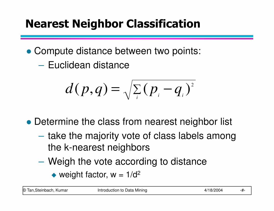
� Compute distance between two points:
– Euclidean distance
� Determine the class from nearest neighbor list
– take the majority vote of class labels among the k-nearest neighbors
– Weigh the vote according to distance
� weight factor, w = 1/d2
∑ −=i ii
qpqpd2)(),(

© Tan,Steinbach, Kumar Introduction to Data Mining 4/18/2004 ‹#›
Nearest Neighbor Classification…
� Choosing the value of k:
– If k is too small, sensitive to noise points
– If k is too large, neighborhood may include points from other classes
© Tan,Steinbach, Kumar Introduction to Data Mining 4/18/2004 ‹#›
Nearest Neighbor Classification…
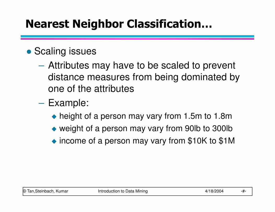
� Scaling issues
– Attributes may have to be scaled to prevent distance measures from being dominated by one of the attributes
– Example:
� height of a person may vary from 1.5m to 1.8m
� weight of a person may vary from 90lb to 300lb
� income of a person may vary from $10K to $1M
© Tan,Steinbach, Kumar Introduction to Data Mining 4/18/2004 ‹#›
Nearest Neighbor Classification…
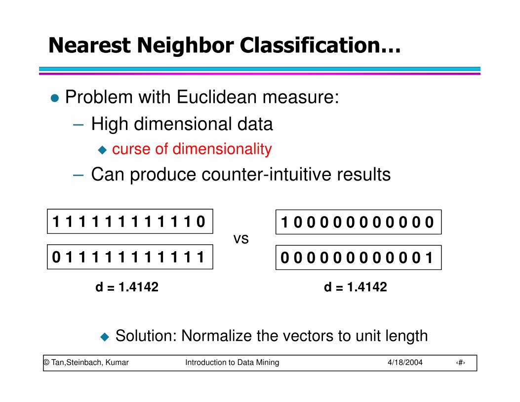
� Problem with Euclidean measure:
– High dimensional data
� curse of dimensionality
– Can produce counter-intuitive results
1 1 1 1 1 1 1 1 1 1 1 0
0 1 1 1 1 1 1 1 1 1 1 1
1 0 0 0 0 0 0 0 0 0 0 0
0 0 0 0 0 0 0 0 0 0 0 1
vs
d = 1.4142 d = 1.4142
� Solution: Normalize the vectors to unit length

© Tan,Steinbach, Kumar Introduction to Data Mining 4/18/2004 ‹#›
Nearest neighbor Classification…
� k-NN classifiers are lazy learners
– It does not build models explicitly
– Unlike eager learners such as decision tree induction and rule-based systems
– Classifying unknown records are relatively expensive
© Tan,Steinbach, Kumar Introduction to Data Mining 4/18/2004 ‹#›
Example: PEBLS
� PEBLS: Parallel Examplar-Based Learning System (Cost & Salzberg)
– Works with both continuous and nominal features
�For nominal features, distance between two nominal values is computed using modified value difference metric (MVDM)
– Each record is assigned a weight factor
– Number of nearest neighbor, k = 1

© Tan,Steinbach, Kumar Introduction to Data Mining 4/18/2004 ‹#›
Example: PEBLS
Class
Marital Status
Single Married Divorced
Yes 2 0 1
No 2 4 1
∑ −=i
ii
n
n
n
nVVd
2
2
1
121 ),(
Distance between nominal attribute values:
d(Single,Married)
= | 2/4 – 0/4 | + | 2/4 – 4/4 | = 1
d(Single,Divorced)
= | 2/4 – 1/2 | + | 2/4 – 1/2 | = 0
d(Married,Divorced)
= | 0/4 – 1/2 | + | 4/4 – 1/2 | = 1
d(Refund=Yes,Refund=No)
= | 0/3 – 3/7 | + | 3/3 – 4/7 | = 6/7
Tid Refund MaritalStatus
TaxableIncome Cheat
1 Yes Single 125K No
2 No Married 100K No
3 No Single 70K No
4 Yes Married 120K No
5 No Divorced 95K Yes
6 No Married 60K No
7 Yes Divorced 220K No
8 No Single 85K Yes
9 No Married 75K No
10 No Single 90K Yes10
Class
Refund
Yes No
Yes 0 3
No 3 4

© Tan,Steinbach, Kumar Introduction to Data Mining 4/18/2004 ‹#›
Example: PEBLS
∑=
=∆d
i
iiYX YXdwwYX1
2),(),(
Tid Refund Marital Status
Taxable Income Cheat
X Yes Single 125K No
Y No Married 100K No 10
Distance between record X and record Y:
where:
correctly predicts X timesofNumber
predictionfor used is X timesofNumber =Xw
wX ≅ 1 if X makes accurate prediction most of the time
wX > 1 if X is not reliable for making predictions
© Tan,Steinbach, Kumar Introduction to Data Mining 4/18/2004 ‹#›
Bayes Classifier
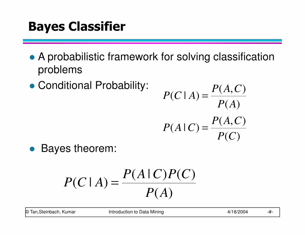
� A probabilistic framework for solving classification problems
� Conditional Probability:
� Bayes theorem:
)(
)()|()|(
AP
CPCAPACP =
)(
),()|(
)(
),()|(
CP
CAPCAP
AP
CAPACP
=
=

© Tan,Steinbach, Kumar Introduction to Data Mining 4/18/2004 ‹#›
Example of Bayes Theorem
� Given: – A doctor knows that meningitis causes stiff neck 50% of the
time
– Prior probability of any patient having meningitis is 1/50,000
– Prior probability of any patient having stiff neck is 1/20
� If a patient has stiff neck, what’s the probability he/she has meningitis?
0002.020/1
50000/15.0
)(
)()|()|( =
×==
SP
MPMSPSMP

© Tan,Steinbach, Kumar Introduction to Data Mining 4/18/2004 ‹#›
Bayesian Classifiers
� Consider each attribute and class label as random variables
� Given a record with attributes (A1, A2,…,An)
– Goal is to predict class C
– Specifically, we want to find the value of C that maximizes P(C| A1, A2,…,An )
� Can we estimate P(C| A1, A2,…,An ) directly from data?

© Tan,Steinbach, Kumar Introduction to Data Mining 4/18/2004 ‹#›
Bayesian Classifiers
� Approach:
– compute the posterior probability P(C | A1, A2, …, An) for all values of C using the Bayes theorem
– Choose value of C that maximizes P(C | A1, A2, …, An)
– Equivalent to choosing value of C that maximizesP(A1, A2, …, An|C) P(C)
� How to estimate P(A1, A2, …, An | C )?
)(
)()|()|(
21
21
21
n
n
n
AAAP
CPCAAAPAAACP
K
K
K =

© Tan,Steinbach, Kumar Introduction to Data Mining 4/18/2004 ‹#›
Naïve Bayes Classifier
� Assume independence among attributes Ai when class is given:
– P(A1, A2, …, An |C) = P(A1| Cj) P(A2| Cj)… P(An| Cj)
– Can estimate P(Ai| Cj) for all Ai and Cj.
– New point is classified to Cj if P(Cj) Π P(Ai| Cj) is maximal.
© Tan,Steinbach, Kumar Introduction to Data Mining 4/18/2004 ‹#›
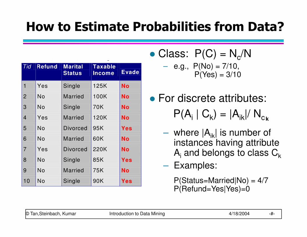
How to Estimate Probabilities from Data?
� Class: P(C) = Nc/N– e.g., P(No) = 7/10,
P(Yes) = 3/10
� For discrete attributes:
P(Ai | Ck) = |Aik|/ Nc
– where |Aik| is number of instances having attribute Ai and belongs to class Ck
– Examples:
P(Status=Married|No) = 4/7P(Refund=Yes|Yes)=0
k
Tid Refund Marital Status
Taxable Income Evade
1 Yes Single 125K No
2 No Married 100K No
3 No Single 70K No
4 Yes Married 120K No
5 No Divorced 95K Yes
6 No Married 60K No
7 Yes Divorced 220K No
8 No Single 85K Yes
9 No Married 75K No
10 No Single 90K Yes 10
categoric
al
categoric
al
continuous
class

© Tan,Steinbach, Kumar Introduction to Data Mining 4/18/2004 ‹#›
How to Estimate Probabilities from Data?
� For continuous attributes:
– Discretize the range into bins � one ordinal attribute per bin
� violates independence assumption
– Two-way split: (A < v) or (A > v)� choose only one of the two splits as new attribute
– Probability density estimation:� Assume attribute follows a normal distribution
� Use data to estimate parameters of distribution (e.g., mean and standard deviation)
� Once probability distribution is known, can use it to estimate the conditional probability P(Ai|c)
k

© Tan,Steinbach, Kumar Introduction to Data Mining 4/18/2004 ‹#›
How to Estimate Probabilities from Data?
� Normal distribution:
– One for each (Ai,ci) pair
� For (Income, Class=No):
– If Class=No
� sample mean = 110
� sample variance = 2975
Tid Refund Marital Status
Taxable Income Evade
1 Yes Single 125K No
2 No Married 100K No
3 No Single 70K No
4 Yes Married 120K No
5 No Divorced 95K Yes
6 No Married 60K No
7 Yes Divorced 220K No
8 No Single 85K Yes
9 No Married 75K No
10 No Single 90K Yes 10
categoric
al
categoric
al
continuous
class
2
2
2
)(
22
1)|( ij
ijiA
ij
jiecAP
σ
µ
πσ
−−
=
0072.0)54.54(2
1)|120( )2975(2
)110120(2
===−
−
eNoIncomePπ

© Tan,Steinbach, Kumar Introduction to Data Mining 4/18/2004 ‹#›
Example of Naïve Bayes Classifier
P(Refund=Yes|No) = 3/7P(Refund=No|No) = 4/7P(Refund=Yes|Yes) = 0P(Refund=No|Yes) = 1P(Marital Status=Single|No) = 2/7P(Marital Status=Divorced|No)=1/7P(Marital Status=Married|No) = 4/7P(Marital Status=Single|Yes) = 2/7P(Marital Status=Divorced|Yes)=1/7P(Marital Status=Married|Yes) = 0
For taxable income:If class=No: sample mean=110
sample variance=2975If class=Yes: sample mean=90
sample variance=25
naive Bayes Classifier:
120K)IncomeMarried,No,Refund( ===X
� P(X|Class=No) = P(Refund=No|Class=No)× P(Married| Class=No)× P(Income=120K| Class=No)
= 4/7 × 4/7 × 0.0072 = 0.0024
� P(X|Class=Yes) = P(Refund=No| Class=Yes)× P(Married| Class=Yes)× P(Income=120K| Class=Yes)
= 1 × 0 × 1.2 × 10-9 = 0
Since P(X|No)P(No) > P(X|Yes)P(Yes)
Therefore P(No|X) > P(Yes|X)
=> Class = No
Given a Test Record:
© Tan,Steinbach, Kumar Introduction to Data Mining 4/18/2004 ‹#›
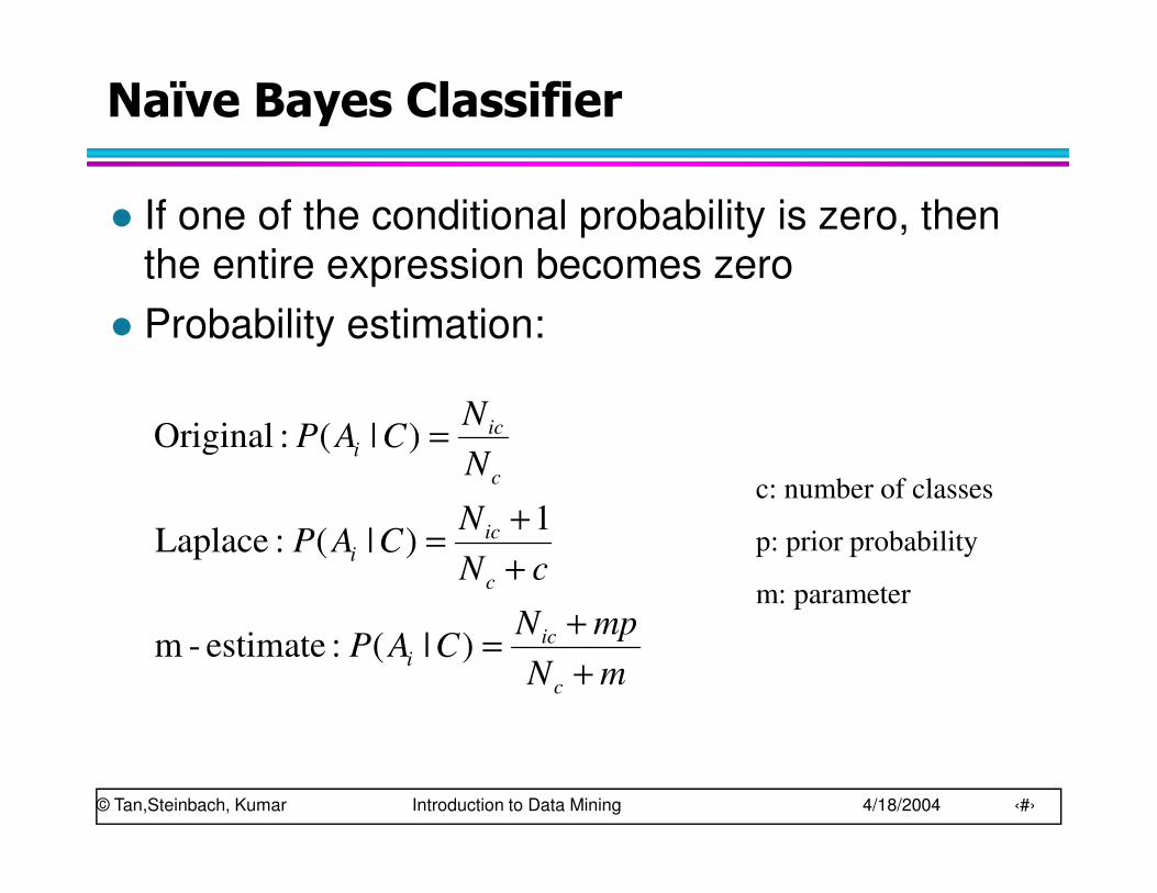
Naïve Bayes Classifier
� If one of the conditional probability is zero, then the entire expression becomes zero
� Probability estimation:
mN
mpNCAP
cN
NCAP
N
NCAP
c
ici
c
ici
c
ici
+
+=
+
+=
=
)|(:estimate-m
1)|(:Laplace
)|( :Original
c: number of classes
p: prior probability
m: parameter
© Tan,Steinbach, Kumar Introduction to Data Mining 4/18/2004 ‹#›
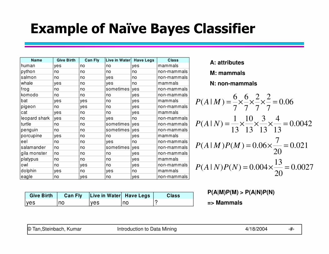
Example of Naïve Bayes Classifier
Name Give Birth Can Fly Live in Water Have Legs Class
human yes no no yes mammals
python no no no no non-mammals
salmon no no yes no non-mammals
whale yes no yes no mammals
frog no no sometimes yes non-mammals
komodo no no no yes non-mammals
bat yes yes no yes mammals
pigeon no yes no yes non-mammals
cat yes no no yes mammals
leopard shark yes no yes no non-mammals
turtle no no sometimes yes non-mammals
penguin no no sometimes yes non-mammals
porcupine yes no no yes mammals
eel no no yes no non-mammals
salamander no no sometimes yes non-mammals
gila monster no no no yes non-mammals
platypus no no no yes mammals
owl no yes no yes non-mammals
dolphin yes no yes no mammals
eagle no yes no yes non-mammals
Give Birth Can Fly Live in Water Have Legs Class
yes no yes no ?
0027.020
13004.0)()|(
021.020
706.0)()|(
0042.013
4
13
3
13
10
13
1)|(
06.07
2
7
2
7
6
7
6)|(
=×=
=×=
=×××=
=×××=
NPNAP
MPMAP
NAP
MAP
A: attributes
M: mammals
N: non-mammals
P(A|M)P(M) > P(A|N)P(N)
=> Mammals

© Tan,Steinbach, Kumar Introduction to Data Mining 4/18/2004 ‹#›
Naïve Bayes (Summary)
� Robust to isolated noise points
� Handle missing values by ignoring the instance during probability estimate calculations
� Robust to irrelevant attributes
� Independence assumption may not hold for some attributes
– Use other techniques such as Bayesian Belief Networks (BBN)
© Tan,Steinbach, Kumar Introduction to Data Mining 4/18/2004 ‹#›
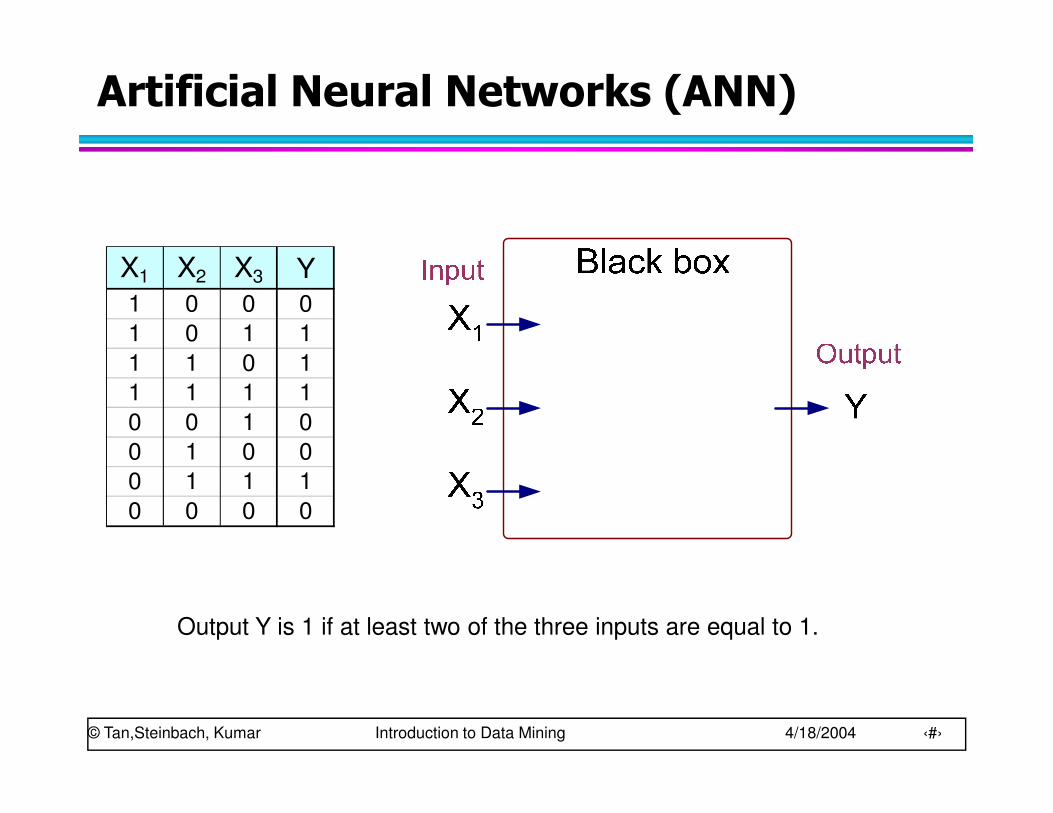
Artificial Neural Networks (ANN)
X1 X2 X3 Y1 0 0 0
1 0 1 1
1 1 0 1
1 1 1 1
0 0 1 0
0 1 0 0
0 1 1 1
0 0 0 0
Output Y is 1 if at least two of the three inputs are equal to 1.

© Tan,Steinbach, Kumar Introduction to Data Mining 4/18/2004 ‹#›
Artificial Neural Networks (ANN)
X1 X2 X3 Y1 0 0 0
1 0 1 1
1 1 0 1
1 1 1 1
0 0 1 0
0 1 0 0
0 1 1 1
0 0 0 0
=
>−++=
otherwise0
trueis if1)( where
)04.03.03.03.0( 321
zzI
XXXIY

© Tan,Steinbach, Kumar Introduction to Data Mining 4/18/2004 ‹#›
Artificial Neural Networks (ANN)
� Model is an assembly of inter-connected nodes and weighted links
� Output node sums up each of its input value according to the weights of its links
� Compare output node against some threshold t
)( tXwIYi
ii −= ∑
Perceptron Model
)( tXwsignYi
ii −= ∑
or

© Tan,Steinbach, Kumar Introduction to Data Mining 4/18/2004 ‹#›
General Structure of ANN
Training ANN means learning the weights of the neurons

© Tan,Steinbach, Kumar Introduction to Data Mining 4/18/2004 ‹#›
Algorithm for learning ANN
� Initialize the weights (w0, w1, …, wk)
� Adjust the weights in such a way that the output of ANN is consistent with class labels of training examples
– Objective function:
– Find the weights wi’s that minimize the above objective function
� e.g., backpropagation algorithm (see lecture notes)
[ ]2),(∑ −=
i
iii XwfYE

© Tan,Steinbach, Kumar Introduction to Data Mining 4/18/2004 ‹#›
Support Vector Machines
� Find a linear hyperplane (decision boundary) that will separate the data

© Tan,Steinbach, Kumar Introduction to Data Mining 4/18/2004 ‹#›
Support Vector Machines
� One Possible Solution
© Tan,Steinbach, Kumar Introduction to Data Mining 4/18/2004 ‹#›
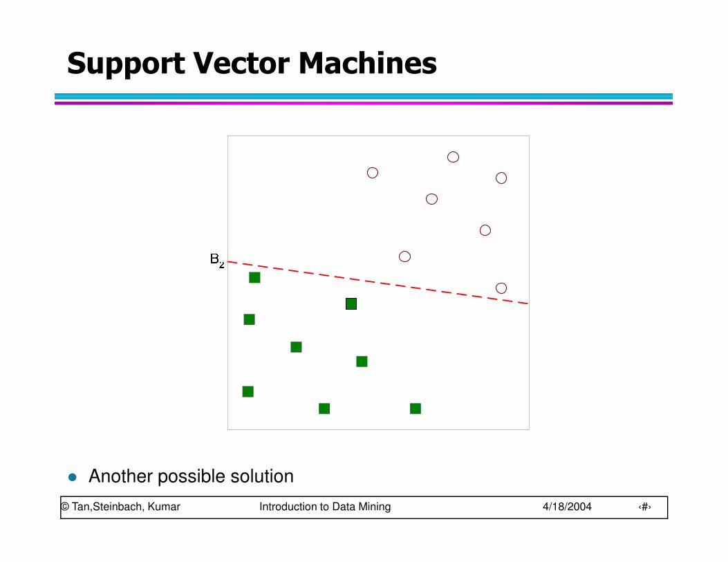
Support Vector Machines
� Another possible solution

© Tan,Steinbach, Kumar Introduction to Data Mining 4/18/2004 ‹#›
Support Vector Machines
� Other possible solutions

© Tan,Steinbach, Kumar Introduction to Data Mining 4/18/2004 ‹#›
Support Vector Machines
� Which one is better? B1 or B2?
� How do you define better?

© Tan,Steinbach, Kumar Introduction to Data Mining 4/18/2004 ‹#›
Support Vector Machines
� Find hyperplane maximizes the margin => B1 is better than B2

© Tan,Steinbach, Kumar Introduction to Data Mining 4/18/2004 ‹#›
Support Vector Machines
0=+• bxwrr
1−=+• bxwrr 1+=+• bxw
rr
−≤+•−
≥+•=
1bxw if1
1bxw if1)(
rr
rr
r
xf 2||||
2 Margin
wr
=

© Tan,Steinbach, Kumar Introduction to Data Mining 4/18/2004 ‹#›
Support Vector Machines
� We want to maximize:
– Which is equivalent to minimizing:
– But subjected to the following constraints:
� This is a constrained optimization problem
– Numerical approaches to solve it (e.g., quadratic programming)
2||||
2 Margin
wr
=
−≤+•−
≥+•=
1bxw if1
1bxw if1)(
i
irr
rr
r
ixf
2
||||)(
2w
wL
r
=

© Tan,Steinbach, Kumar Introduction to Data Mining 4/18/2004 ‹#›
Support Vector Machines
� What if the problem is not linearly separable?

© Tan,Steinbach, Kumar Introduction to Data Mining 4/18/2004 ‹#›
Support Vector Machines
� What if the problem is not linearly separable?
– Introduce slack variables
� Need to minimize:
� Subject to:
+−≤+•−
≥+•=
ii
ii
1bxw if1
-1bxw if1)(
ξ
ξrr
rr
r
ixf
+= ∑
=
N
i
k
iCw
wL1
2
2
||||)( ξ
r
© Tan,Steinbach, Kumar Introduction to Data Mining 4/18/2004 ‹#›
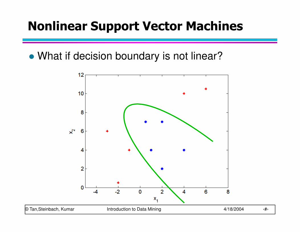
Nonlinear Support Vector Machines
� What if decision boundary is not linear?

© Tan,Steinbach, Kumar Introduction to Data Mining 4/18/2004 ‹#›
Nonlinear Support Vector Machines
� Transform data into higher dimensional space
© Tan,Steinbach, Kumar Introduction to Data Mining 4/18/2004 ‹#›
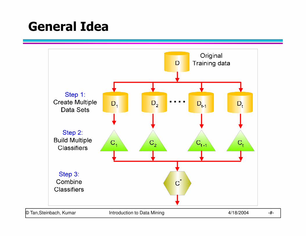
Ensemble Methods
� Construct a set of classifiers from the training data
� Predict class label of previously unseen records by aggregating predictions made by multiple classifiers
© Tan,Steinbach, Kumar Introduction to Data Mining 4/18/2004 ‹#›
General Idea

© Tan,Steinbach, Kumar Introduction to Data Mining 4/18/2004 ‹#›
Why does it work?
� Suppose there are 25 base classifiers
– Each classifier has error rate, ε = 0.35
– Assume classifiers are independent
– Probability that the ensemble classifier makes a wrong prediction:
∑=
− =−
25
13
25 06.0)1(25
i
ii
iεε

© Tan,Steinbach, Kumar Introduction to Data Mining 4/18/2004 ‹#›
Examples of Ensemble Methods
� How to generate an ensemble of classifiers?
– Bagging
– Boosting

© Tan,Steinbach, Kumar Introduction to Data Mining 4/18/2004 ‹#›
Bagging
� Sampling with replacement
� Build classifier on each bootstrap sample
� Each sample has probability (1 – 1/n)n of being selected
Original Data 1 2 3 4 5 6 7 8 9 10Bagging (Round 1) 7 8 10 8 2 5 10 10 5 9Bagging (Round 2) 1 4 9 1 2 3 2 7 3 2Bagging (Round 3) 1 8 5 10 5 5 9 6 3 7

© Tan,Steinbach, Kumar Introduction to Data Mining 4/18/2004 ‹#›
Boosting
� An iterative procedure to adaptively change distribution of training data by focusing more on previously misclassified records
– Initially, all N records are assigned equal weights
– Unlike bagging, weights may change at the end of boosting round

© Tan,Steinbach, Kumar Introduction to Data Mining 4/18/2004 ‹#›
Boosting
� Records that are wrongly classified will have their weights increased
� Records that are classified correctly will have their weights decreased
Original Data 1 2 3 4 5 6 7 8 9 10Boosting (Round 1) 7 3 2 8 7 9 4 10 6 3Boosting (Round 2) 5 4 9 4 2 5 1 7 4 2Boosting (Round 3) 4 4 8 10 4 5 4 6 3 4
• Example 4 is hard to classify
• Its weight is increased, therefore it is more likely to be chosen again in subsequent rounds
© Tan,Steinbach, Kumar Introduction to Data Mining 4/18/2004 ‹#›
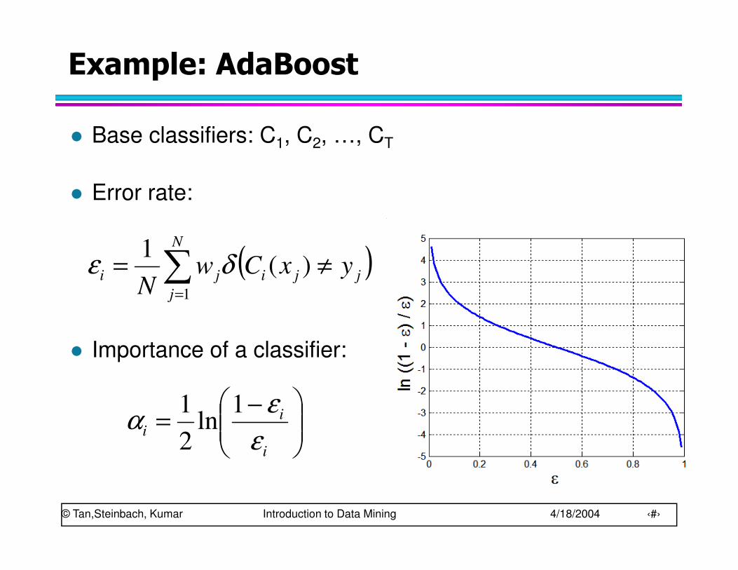
Example: AdaBoost
� Base classifiers: C1, C2, …, CT
� Error rate:
� Importance of a classifier:
( )∑=
≠=N
j
jjiji yxCwN 1
)(1
δε
−=
i
ii
ε
εα
1ln
2
1
© Tan,Steinbach, Kumar Introduction to Data Mining 4/18/2004 ‹#›
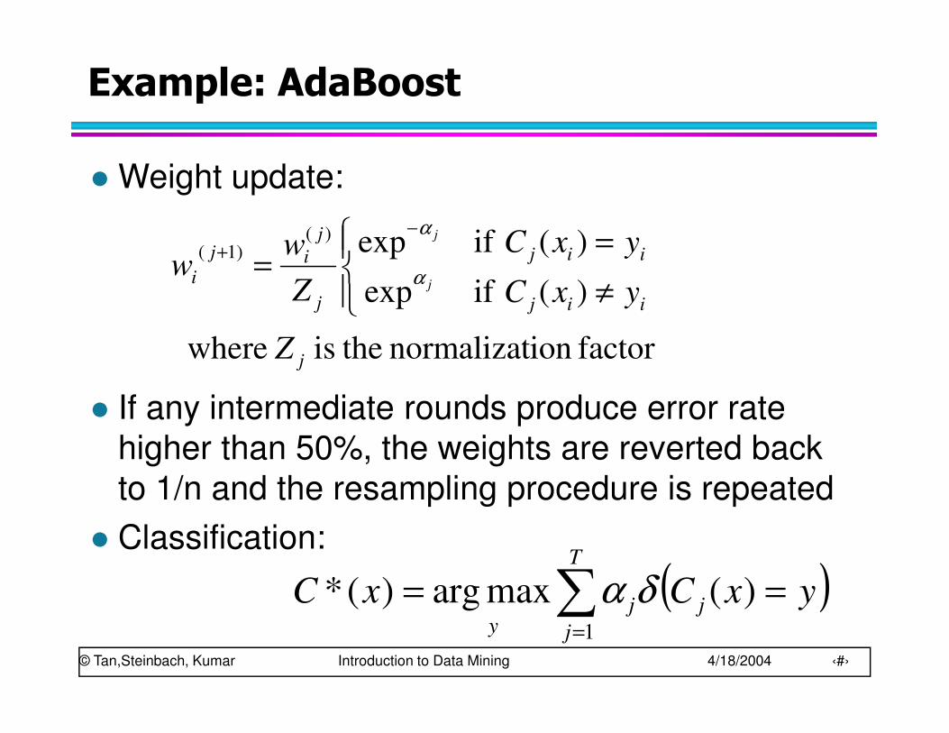
Example: AdaBoost
� Weight update:
� If any intermediate rounds produce error rate higher than 50%, the weights are reverted back to 1/n and the resampling procedure is repeated
� Classification:
factor ionnormalizat theis where
)( ifexp
)( ifexp)()1(
j
iij
iij
j
j
ij
i
Z
yxC
yxC
Z
ww
j
j
≠
==
−
+
α
α
( )∑=
==T
j
jjy
yxCxC1
)(maxarg)(* δα

© Tan,Steinbach, Kumar Introduction to Data Mining 4/18/2004 ‹#›
Illustrating AdaBoost
Data points for training
Initial weights for each data point

© Tan,Steinbach, Kumar Introduction to Data Mining 4/18/2004 ‹#›
Illustrating AdaBoost