data mining and optimization in steam-assisted gravity
TRANSCRIPT

Data Mining and Optimization in Steam-assisted gravity drainageprocess
by
Chaoqun Li
A thesis submitted in partial fulfillment of the requirements for the degree of
Master of Science
in
Process Control
Department of Chemical and Materials Engineering
University of Alberta
©Chaoqun Li, 2018
Abstract
Steam-assisted gravity drainage (SAGD) is an enhanced oil recovery (EOR) technol-
ogy widely used in Canada. Data available in SAGD industrial processes contain
valuable information for monitoring, soft sensing, control, and optimization. This
thesis focuses on data mining and optimization in the SAGD process, including the
comparative study of machine learning algorithms, Bayesian Optimization and soft
sensor design.
Subcool is a key variable of SAGD, that is important for safety and efficiency. The
popular machine learning algorithms, especially those having good practical merit,
are tested and compared in a subcool monitoring case. The advantages of multiple
machine learning algorithms are analyzed and discussed. Moreover, investigating the
original dataset suggests that data quality and priori knowledge play a vital role in
applying machine learning to study data analytics problems to oil sands industry.
Bayesian Optimization considers model building and optimization simultaneously.
Locally weighted quadratic regression is incorporated into the Bayesian Optimization
framework, serving as the surrogate model. Details of the existing framework are
tailored to use locally weighted quadratic regression as the surrogate model. Numeri-
cal cases are tested to demonstrate the usefulness of the Locally Weighted Quadratic
Regression based Bayesian Optimization (LWQRBO). Additionally, the application
of the proposed LWQRBO to address the formulated SAGD optimization problem
is explored. Finally, optimization results show the applicability of LWQRBO in the
SAGD process.
Soft sensing constructs models with data mining approaches. It is an alternative
way to measure process variables when hardware sensors are not available. Stacking
online soft sensor is designed for the SAGD process. The idea of stacking models
inspires this design which applies multiple linear regression as a second level model,
ii

considering ease of implementation. Two cases are studied to show the applicability
and suitability of the designed soft sensor in the SAGD process.
The topics of Bayesian Optimization and ensemble models for soft sensor extend
promising research directions. They are presented at the end of this thesis.
iii

Preface
The materials presented in the thesis are part of the research project under the
supervision of Professor Biao Huang and are funded by Alberta Innovates Technology
Futures (AITF) and the Natural Sciences and Engineering Research Council (NSERC)
of Canada.
A version of Chapter 2 of the thesis was submitted to the 10th IFAC Symposium
on Advanced Control of Chemical Processes Conference. I was responsible for concept
formation, program coding, data analysis, drawing conclusion as well as manuscript
composition. Nabil Magbool Jan was involved in concept formation, data analysis
and contributed to manuscript edits. Dr. Biao Huang was the supervisory author
and was involved in manuscript composition.
iv

Acknowledgements
First and foremost, it gives me great pleasure to acknowledge my supervisor, Dr.
Biao Huang. He gave me the opportunity to explore my way in the awesome and
excellent Computer Process Control (CPC) group. Dr. Biao Huang is always there
to help in research. He guided me while I was trapped and lost in a research problem,
encouraged me while I lost confidence, and gave me useful suggestions while I was
confused about what to do next. Dr. Biao Huang is not only a professional supervisor
in my research but also a life coach in how to get things done and how to live a happy
life.
I appreciate Dr. Zukui Li and Dr. Csaba Szepesvari. They gave me valuable
suggestions during my research. I also would like to give my thank to Nabil Magbool
Jan, who had been discussing with me and helping me in the whole journey of research.
I am also very grateful to Yuan Yuan, Mohammad Rashedi, Yanjun Ma, Wenhan
Shen, Ruomu Tan and Seraphina Kwak. They were so helpful to me on discussing
research topics, sharing ideas and figuring out solutions.
I would like give my great thank to Ming Ma and Yaojie Lu, who helped me while
I was making an application to Graduate Study at University of Alberta. During
my study here, I have met my exceptional CPC group members as well as those who
have graduated. I next would like to thank my collegues and friends, they are: Lei
Fan, Mengqi Fang, Guoyang Yan, Gary Wang, Hashem Alighardashi, Atefeh Daemi,
Zheyuan Liu, Fadi Ibrahim, Ruoxia Li, Rahul Raveendran, Shabnam Sedghi, Agustin
Vicente, Anahita Sadeghian, Alireza Kheradmand, Yousef Alipouri and Kirubakaran
Velswamy. I also want to thank our visiting scholars and graduated group members:
Chen Xu, Ouyang Wu, Yujia Zhao, Rishik Ranjan, Yan Qin, Shunyi Zhao and Junxia
Ma.
Last but not least, I owe my deepest gratitude to my parents.
v

Contents
1 Introduction 1
1.1 Motivation . . . . . . . . . . . . . . . . . . . . . . . . . . . . . . . . . 1
1.2 Thesis Contributions . . . . . . . . . . . . . . . . . . . . . . . . . . . 2
1.3 Thesis Outline . . . . . . . . . . . . . . . . . . . . . . . . . . . . . . . 3
2 Data analytics for oil sands subcool prediction - a comparative study
of machine learning algorithms 5
2.1 Introduction . . . . . . . . . . . . . . . . . . . . . . . . . . . . . . . . 5
2.2 Problem description . . . . . . . . . . . . . . . . . . . . . . . . . . . . 7
2.3 Revisiting selected machine learning methods . . . . . . . . . . . . . 8
2.3.1 Deep Learning . . . . . . . . . . . . . . . . . . . . . . . . . . . 8
2.3.2 Gradient Boosted Decision Trees . . . . . . . . . . . . . . . . 9
2.3.3 Random Forest . . . . . . . . . . . . . . . . . . . . . . . . . . 10
2.3.4 Support Vector Regression . . . . . . . . . . . . . . . . . . . . 11
2.3.5 Linear Regression and Ridge Regression . . . . . . . . . . . . 11
2.4 Model Development . . . . . . . . . . . . . . . . . . . . . . . . . . . . 11
2.4.1 Data Description . . . . . . . . . . . . . . . . . . . . . . . . . 12
2.4.2 Data Pre-processing . . . . . . . . . . . . . . . . . . . . . . . 12
2.4.3 Hyperparameter exploration . . . . . . . . . . . . . . . . . . . 13
2.4.4 Software and Platform . . . . . . . . . . . . . . . . . . . . . . 16
2.5 Results and discussions . . . . . . . . . . . . . . . . . . . . . . . . . . 17
2.5.1 Performance on test data . . . . . . . . . . . . . . . . . . . . . 17
2.5.2 Discussion . . . . . . . . . . . . . . . . . . . . . . . . . . . . . 21
2.6 Data quality and priori knowledge play a vital role . . . . . . . . . . 22
2.6.1 Case Study on a different dataset . . . . . . . . . . . . . . . . 23
vi

2.6.2 Investigation to original dataset and analysis . . . . . . . . . . 28
2.7 Conclusions . . . . . . . . . . . . . . . . . . . . . . . . . . . . . . . . 29
3 Locally Weighted Quadratic Regression based Bayesian Optimiza-
tion and its application in SAGD process 30
3.1 Literature Review of Bayesian Optimization . . . . . . . . . . . . . . 30
3.2 Locally Weighted Quadratic Regression based Bayesian Optimization 32
3.2.1 Efficient Global Optimization . . . . . . . . . . . . . . . . . . 33
3.2.2 Locally Weighted Learning . . . . . . . . . . . . . . . . . . . . 35
3.2.3 Locally Weighted Quadratic Regression based Bayesian Opti-
mization . . . . . . . . . . . . . . . . . . . . . . . . . . . . . . 37
3.3 Case Study . . . . . . . . . . . . . . . . . . . . . . . . . . . . . . . . 42
3.3.1 Case Study 1 . . . . . . . . . . . . . . . . . . . . . . . . . . . 43
3.3.2 Case Study 2 . . . . . . . . . . . . . . . . . . . . . . . . . . . 46
3.4 Application in simulated SAGD process . . . . . . . . . . . . . . . . . 48
3.4.1 SAGD Optimization Review . . . . . . . . . . . . . . . . . . . 49
3.4.2 Motivation and Problem Description . . . . . . . . . . . . . . 50
3.4.3 Optimization Results . . . . . . . . . . . . . . . . . . . . . . . 53
3.5 Conclusions . . . . . . . . . . . . . . . . . . . . . . . . . . . . . . . . 57
4 Stacking online soft sensor application in SAGD process 58
4.1 Review of soft sensor design approaches . . . . . . . . . . . . . . . . . 58
4.2 A brief introduction to the idea of stacking models . . . . . . . . . . 60
4.3 Revisit of Partial Least Squares Regression, Gaussian Process Regres-
sion and Support Vector Regression . . . . . . . . . . . . . . . . . . . 61
4.3.1 Partial Least Squares Regression . . . . . . . . . . . . . . . . 62
4.3.2 Gaussian Process Regression . . . . . . . . . . . . . . . . . . . 62
4.3.3 Support Vector Regression . . . . . . . . . . . . . . . . . . . . 63
4.4 Design of stacking online soft sensor for SAGD process . . . . . . . . 64
4.4.1 Design of the proposed soft sensor . . . . . . . . . . . . . . . . 64
4.4.2 Practicability and scalability of the designed soft sensor . . . . 67
4.5 Application of stacking online soft sensor in SAGD process . . . . . . 68
vii

4.5.1 Case Study 1: Automatic Model Switching . . . . . . . . . . . 68
4.5.2 Case Study 2: Model Performance Improvement . . . . . . . . 75
4.6 Conclusions . . . . . . . . . . . . . . . . . . . . . . . . . . . . . . . . 77
5 Conclusions 78
5.1 Summary of This Thesis . . . . . . . . . . . . . . . . . . . . . . . . . 78
5.2 Directions for Future Work . . . . . . . . . . . . . . . . . . . . . . . . 79
viii

List of Tables
2.1 Variable description for subcool prediction . . . . . . . . . . . . . . . 12
2.2 Hyperparameter settings, Deep Learning/Deep Feedforward Neural
Networks . . . . . . . . . . . . . . . . . . . . . . . . . . . . . . . . . . 14
2.3 Hyperparameter settings, GBDT . . . . . . . . . . . . . . . . . . . . 15
2.4 Hyperparameter settings, Random Forest . . . . . . . . . . . . . . . . 15
2.5 Hyperparameter settings, Support Vector Regression . . . . . . . . . 16
2.6 Hyperparameter settings, Ridge Regression . . . . . . . . . . . . . . . 16
2.7 Test results . . . . . . . . . . . . . . . . . . . . . . . . . . . . . . . . 17
2.8 Statistics of Deep Learning/Deep Feedforward Networks results of Sec-
tion 2.5.1 . . . . . . . . . . . . . . . . . . . . . . . . . . . . . . . . . 21
2.9 Hyperparameter settings of new dataset, Deep Learning/Deep Feed-
forward Neural Networks . . . . . . . . . . . . . . . . . . . . . . . . . 23
2.10 Hyperparameter settings of new dataset, GBDT . . . . . . . . . . . . 23
2.11 Hyperparameter settings of new dataset, Random Forest . . . . . . . 24
2.12 Hyperparameter settings of new dataset, Support Vector Regression . 24
2.13 Hyperparameter settings of new dataset, Ridge Regression . . . . . . 24
2.14 Test results of new dataset . . . . . . . . . . . . . . . . . . . . . . . . 24
3.1 Reservoir Parameters . . . . . . . . . . . . . . . . . . . . . . . . . . . 54
3.2 Operational Bounded Constraints . . . . . . . . . . . . . . . . . . . . 54
4.1 Description of variables of simulated dataset . . . . . . . . . . . . . . 70
4.2 Statistical metrics on test data in Period 1 . . . . . . . . . . . . . . . 71
4.3 Statistical metrics on test data in Period 2 . . . . . . . . . . . . . . . 73
4.4 Statistical metrics on test data in Period 3 . . . . . . . . . . . . . . . 74
4.5 Statistical metrics on industrial test data . . . . . . . . . . . . . . . . 76
ix

List of Figures
2.1 Process description . . . . . . . . . . . . . . . . . . . . . . . . . . . . 8
2.2 Architecture of Deep Feedforward Neural Networks . . . . . . . . . . 14
2.3 Test results of Deep Learning/Deep Feedforward Neural Networks . . 18
2.4 Test results of Gradient Boosted Decision Tree . . . . . . . . . . . . . 18
2.5 Test results of Random Forest . . . . . . . . . . . . . . . . . . . . . . 19
2.6 Test results of Support Vector Regression . . . . . . . . . . . . . . . . 19
2.7 Test results of Ridge Regression . . . . . . . . . . . . . . . . . . . . . 20
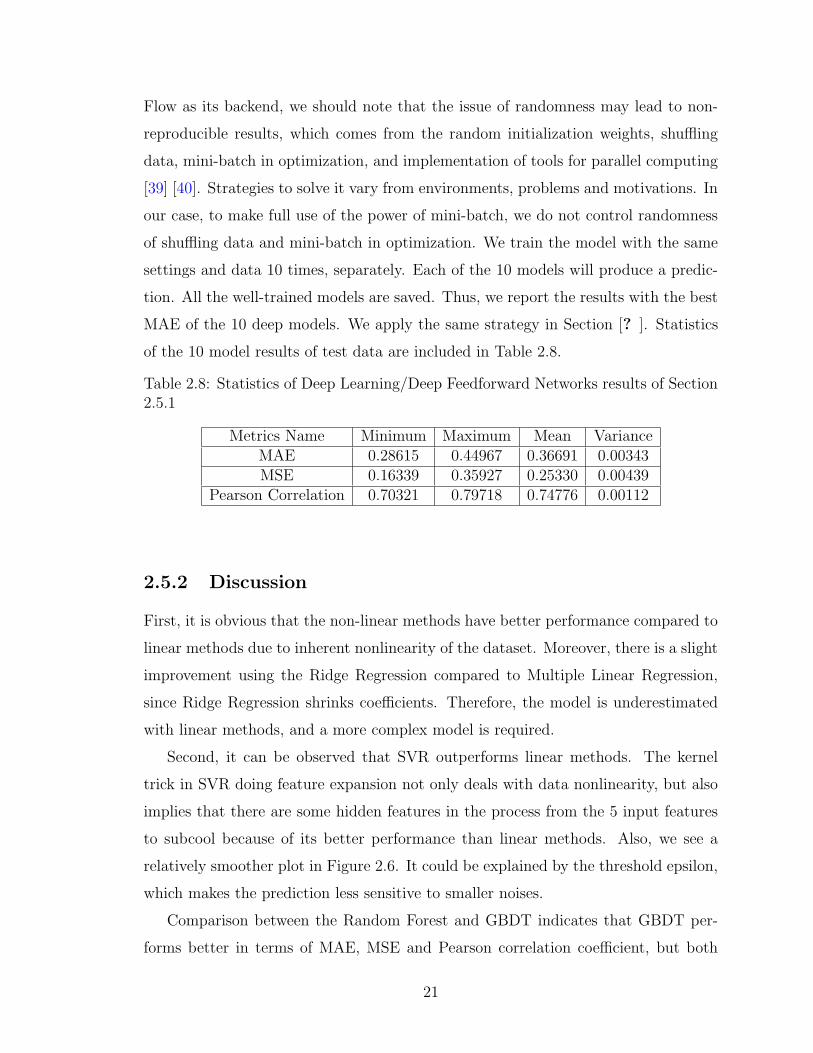
2.8 Test results of Multiple Linear Regression . . . . . . . . . . . . . . . 20
2.9 Test results of Deep Learning/Deep Feedforward Neural Networks us-
ing new dataset . . . . . . . . . . . . . . . . . . . . . . . . . . . . . . 25
2.10 Test results of GBDT using new dataset . . . . . . . . . . . . . . . . 26
2.11 Test results of Random Forest using new dataset . . . . . . . . . . . . 26
2.12 Test results of Support Vector Regression using new dataset . . . . . 27
2.13 Test results of Ridge Regression using new dataset . . . . . . . . . . . 27
2.14 Test results of Multiple Linear Regression using new dataset . . . . . 28
2.15 Trend of Injection Tubing Pressure . . . . . . . . . . . . . . . . . . . 29
3.1 Sampling without considering model uncertainties . . . . . . . . . . . 33
3.2 Model uncertainties . . . . . . . . . . . . . . . . . . . . . . . . . . . . 34
3.3 Illustration of locally weighted learning . . . . . . . . . . . . . . . . 36
3.4 Flowchart of LWQRBO . . . . . . . . . . . . . . . . . . . . . . . . . 42
3.5 Curve of 1-d test function . . . . . . . . . . . . . . . . . . . . . . . . 43
3.6 Performance through iterations . . . . . . . . . . . . . . . . . . . . . 44
3.7 Expected Improvement of 1-d case . . . . . . . . . . . . . . . . . . . 45
3.8 Locations of sampled points . . . . . . . . . . . . . . . . . . . . . . . 46
x

3.9 Performance through iterations . . . . . . . . . . . . . . . . . . . . . 47
3.10 Expected Improvement of 2-d case . . . . . . . . . . . . . . . . . . . 48
3.11 Schematic of SAGD process . . . . . . . . . . . . . . . . . . . . . . . 51
3.12 Optimization model elements . . . . . . . . . . . . . . . . . . . . . . 52
3.13 SAGD Optimization performance . . . . . . . . . . . . . . . . . . . . 55
3.14 Trend of Expected Improvement . . . . . . . . . . . . . . . . . . . . . 56
3.15 Location of Initial Data and Sampled Data . . . . . . . . . . . . . . . 57
4.1 Schematic of smart online soft sensor . . . . . . . . . . . . . . . . . . 65
4.2 Training and testing data partition along with timeline . . . . . . . . 69
4.3 Performance on test data in Period 1 . . . . . . . . . . . . . . . . . . 71
4.4 Performance on test data in Period 2 . . . . . . . . . . . . . . . . . . 72
4.5 Performance on test data in Period 3 . . . . . . . . . . . . . . . . . . 74
4.6 Performance on industrial test data . . . . . . . . . . . . . . . . . . . 76
xi

Chapter 1
Introduction
1.1 Motivation
Steam-assisted gravity drainage (SAGD) is an enhanced oil recovery technology used
in the extraction of bitumen from a reservoir [1]. The core process of SAGD is de-
scribed as follows [1] [2]: high pressure steam is generated from a steam generator,
the generated steam is then injected into the injection well and flows down to un-
derground. Heat transfer occurs between injected steam and solid bitumen in the
reservoir. Solid bitumen is heated and flows down to the production well due to
gravity. A steam chamber is formed in the reservoir. Bitumen in the production well
is lifted to the surface by a pump for further processing.
In the SAGD process, there exist many key variables [1] [3] such as chamber
pressure, subcool, injection flowrate, injection pressure, etc. These variables are vital
in processing safety and determining economic performance. Further, they play a
critical role in the tasks of monitoring, control and optimization of the SAGD process.
Success of these tasks relies heavily on the accuracy of the models involved in the
process. Owing to complexity of the SAGD process, developing first principles based
models is rather difficult. On the other hand, the oil sands industry has a large
amount of data, which can be utilized to develop reliable data-driven models of the
process. Therefore, in this work, data-driven models are constructed for the SAGD
process.
These data-driven models can be developed for soft sensor applications to perform
monitoring and for prediction. Soft sensors are alternatives to hardware sensors. In
cases where hardware sensors are not available or are shut down for maintenance, soft
1

sensors can be used. Additionally, the data driven models constructed can be used
for optimization [4] [5].
The main focus of this thesis is data mining and optimization in the SAGD process.
This thesis targets data analytics and monitoring of subcool using machine learning
algorithms, Bayesian Optimization to solve SAGD optimization problem, as well as
soft sensor design for the SAGD process.
In each of the three main chapters, prediction models are built. In Chapter 2,
subcool is predicted with multiple machine learning algorithms, all of which are glob-
al models. The regression of SOR is also performed with global models, but the
performance is not satisfying. So, we build locally weighted models in Chapter 3. In
Chapter 4, we still target on global models for soft sensors design, to show the design
idea. More details of each main chapter are introduced in next section.
1.2 Thesis Contributions
This thesis contributes to data mining and optimization in the SAGD process. Mul-
tiple machine learning algorithms are studied for their performance in subcool mon-
itoring. This thesis also proposes the Locally Weighted Quadratic Regression based
Bayesian Optimization (LWQRBO) method. The proposed LWQRBO is then ap-
plied to optimize the SAGD process. A stacking online soft sensor is designed, and
its usefulness in SAGD is presented. Detailed contributions of this work are as follows:
1. A comparative study of multiple machine learning algorithms on SAGD subcool
monitoring is conducted on industrial datasets. Advantages of different algorithms
are discussed.
2. Investigation and analysis of the original industrial dataset of the subcool
monitoring case demonstrate the factors which should be taken into, to apply machine
learning tools in the oil sands industry.
3. A Locally Weighted Learning based Bayesian Optimization method is proposed,
with locally weighted quadratic regression as the surrogate model in the Bayesian
2

Optimization framework. Two numerical test functions are presented to demonstrate
the performance of the proposed LWQRBO approach.
4. An optimization problem of the SAGD process is formulated. The proposed
LWQRBO approach is applied to solve this SAGD optimization problem.
5. A stacking online soft sensor is designed particularly for the SAGD process.
The design details are provided. Two case studies are presented to show the effec-
tiveness of the designed stacking online soft sensor.
1.3 Thesis Outline
The thesis is outlined as follows:
In Chapter 2, the performances of multiple machine learning algorithms in making
subcool predictions with other process variables are compared. Deep Neural Networks
of Deep Learning, Gradient Boosted Decision Trees, Random Forest, Support Vector
Regression, Ridge Regression and Multiple Linear Regression are tested. The results
are presented and the strengths of each of these algorithms are described. Also,
this chapter shows the need for incorporating process knowledge in performing data
analytics in the oil sands industry.
LWQRBO is proposed in Chapter 3, where locally weighted approaches in Bayesian
Optimization with Expected Improvement are applied as the figure of merit. Predic-
tion and standard error of prediction are two components of Expected Improvement
(EI), and those of locally weighted quadratic regression are incorporated into EI. Two
numerical test functions are investigated to elucidate the usefulness of the proposed
approach. A SAGD optimization problem is formulated, and the proposed approach
is applied in a simulated SAGD process to show its applicability.
In Chapter 4, a stacking online soft sensor for the SAGD process is designed. This
soft sensor applies the model stacking idea. Multiple linear regression is used as the
online model, to correct predictions of offline predictive models. Two case studies,
Annual Reservoir Pressure soft sensor and Water Content soft sensor, demonstrate
the feasibility and effectiveness of the designed stacking online soft sensor in SAGD
3

process.
Conclusions and directions for future work are provided in Chapter 5.
4
Chapter 2
Data analytics for oil sands subcoolprediction - a comparative study ofmachine learning algorithms*
In this chapter, we do a comparative study of different machine learning algorithms
on subcool monitoring of the SAGD process. This chapter focuses on developing sub-
cool models with industrial datasets using deep learning and several other widely-used
machine learning methods. In Section 2.1, a literature review of SAGD and subcool
is provided. In Section 2.2, the targeted problem is formulated. Section 2.3 presents
a brief description of deep learning and other selected machine learning methods.
The subcool model development and corresponding hyperparameter exploration are
discussed in Section 2.4. Model performances of different algorithms using industrial
dataset are analyzed in Section 2.5. In Section 2.6, the vital role of data quality and
priori knowledge are demonstrated. Conclusions are presented in Section 2.7.
2.1 Introduction
Steam Assisted Gravity Drainage (SAGD) is an efficient, in situ, enhanced oil re-
covery technique to produce heavy crude oil and bitumen from reservoirs [1]. The
SAGD operation involves a well pair consisting of two wells; an injection well, and
a production well. The high-temperature steam, generated from the steam genera-
*This chapter was modified to have been submitted to the 10th IFAC Symposium on AdvancedControl of Chemical Processes Conference: Chaoqun Li, Nabil Magbool Jan, Biao Huang, Dataanalytics for oil sands subcool prediction a comparative study of machine learning algorithms
5

tion system, is injected into the reservoir through the injection well which heats up
and reduces the viscosity of the heavy bitumen in the reservoir, and forms the steam
chamber underground. The heated bitumen and condensed liquid then flow towards
the production well due to gravity. The bitumen collected in the producer is then
pumped to the surface for further processing [1] [2].
In a recent review paper, the elements of SAGD success, economics and operations,
mechanics and the effects of reservoir properties on SAGD have been extensively
discussed [2]. In addition, the detailed review of Geo-mechanical effect and Steam-
Fingering Theory on SAGD process have been discussed [3].
One of the most important variables in SAGD operations is subcool, which is the
temperature difference between steam at the injector and fluid at the producer [6]. It
is a key parameter which reflects the liquid level at the producer and has a significant
impact on SAGD reservoir performance [6]. Yuan et al. [7] studied the relationship
between subcool, wellbore drawdown, fluid productivity and liquid level. Moreover,
a model for the SAGD liquid pool above the production well was studied with heat
balance and mass balance equations [8].
Ito et al. [9] conducted a study on reservoir dynamics and subcool optimization
for steam trap control. Subcool has been considered an important factor for Artificial
Lift Systems [10]. Gotawala et al. [11] proposed a subcool control method with smart
injection wells. In their study, they divided the SAGD injector into several intervals,
and controlled subcool by changing the steam pressure at each interval. In addition,
the study on the optimization of subcool in SAGD bitumen process has been carried
out [12]. Furthermore, the Model Predictive Control technique has been used to
stabilize subcool temperature and automate well operations in SAGD industry [13]
[14].
Subcool not only influences reservoir and oil production performance but also has
a significant effect on operational safety, since it can reflect the liquid level of the pro-
ducer. An inappropriate liquid level can result in steam breakthrough thus damaging
equipment. Therefore, predicting the subcool value is necessary, and it is beneficial
in monitoring, control, and optimization of the process. From the monitoring point
of view, the prediction model of the subcool can provide useful information to process
and operations engineers. From the control or optimization point of view, the subcool
6

response to the operational variables is important since the subcool value plays a key
role in bitumen production in addition to the steam utilization.
SAGD is a complex thermal recovery process. Since subcool is a temperature
difference, and several factors which have an effect on the temperature at injector
and producer will influence the subcool. For example, pump frequency will influence
the liquid level trapped at the bottom of the producer, therefore, it has an effect on
the temperature at the producer. Also, the heterogeneity of the reservoir properties
hinders us from developing a first principle model of subcool. Researchers, therefore,
often resort to developing data-driven models in this work.
2.2 Problem description
SAGD technology has been used extensively in the oil sands industry in recen-
t decades, and a large volume of historical industrial datasets are available. With
the advent of novel machine learning methods and data analytics, these historical
process data can be efficiently used to improve the process performance. The stored
data contains a wide variety of information such as seismic images of the steam cham-
ber which are of image types and conventional process variables that are stored as
floating point variables. Further, the enhancement in the instrumentation of the op-
erations has increased the speed at which the data is stored. In addition, the data
includes a lot of inconsistent measurement and missing values, which can be caused
by the hardware sensor faults. It also has noisy measurement due to the hardware
sensors and varying environment. Data in SAGD process also contains a lot of useful
information that can be used efficiently to improve the process operation and increase
profitability.
In this study, we aim to solve a problem of estimating an underground state
variable, subcool, using some of the manipulated variables as inputs. Figure 2.1
presents the schematic of SAGD operation. The injected steam plays a significant
role in subcool, and the liquids produced are lifted up by the pump. Therefore, the
input variables used are those related to injector flowrate, injector pressure, and pump
7

frequency. In this study, we will build a prediction model of subcool as follows:
Y = f(X1, X2, ..., Xp) (2.1)
where Y denotes subcool at a certain location and X1, X2, ..., Xp denote selected
input variables. As described, we have only selected manipulated variables as influen-
tial features for the subcool prediction. The developed data-driven model is beneficial
when underground hardware sensor measurement is unavailable or unreliable, and can
be utilized as an alternative sensor measurement.
Figure 2.1: Process description
2.3 Revisiting selected machine learning methods
Machine learning includes a wide range of algorithms, such as supervised learning,
unsupervised learning, reinforcement learning, transfer learning, etc. As described
in Section 2.2, we will focus on solving a modelling problem for a highly complex
industrial process in this work. In order to deal with complex industrial data, we
resort to advanced data-driven modelling techniques. We consider several widely used
algorithms including Deep Learning, ensemble tree-based methods, kernel methods
and linear methods. We introduce them briefly in this section.
2.3.1 Deep Learning
Deep Learning includes a wide range of algorithms, such as Deep Neural Networks,
Auto Encoders, Restricted Boltzmann Machines, Deep Belief Networks, etc. They can
8

perform supervised learning, semi-supervised learning and unsupervised learning [15].
There are many Deep Neural Networks types, such as Convolutional Neural Network
(CNN) and Long Short Term Memory (LSTM), which have profound applications
in Image Processing and Natural Language Processing, respectively [16]. Generative
Adversarial Networks (GAN) is an example of the popular networks which is used in
unsupervised learning algorithm [17].
In this study, we consider Deep feedforward neural networks. “Deep feedforward
networks, also called feedforward neural networks, or multilayer perceptrons (MLPs),
are the quintessential deep learning models” [15]. Multilayer feedforward networks
have been proved to be universal approximators [18].
We next introduce some key aspects of deep feedforward network which are crucial
to its performance. One of the important factors that determine the convergence of a
deep network and its performance is weight initialization. There are several methods
to do the initialization, via randomly sampling from a uniform or normal distribution
over an interval or generating a random orthogonal matrix [19] [20] [21].
Another important factor that affects the performance of a deep learning model
is the choice of the activation function. Sigmoid and hyperbolic tangent function
were the popular choices of activation function in the past, and Rectified Linear Unit
(ReLU) has become popular recently [16]. The mathematical form of ReLU, which is
proved to improve Restricted Boltzmann Machines, can be expressed as follows [22]:
f(x) = max(0, x) (2.2)
There are some variants of ReLUs, such as Leaky ReLUs and Exponential Linear
Units (ELUs) [23] [24].
Another important component in Deep Learning is the optimization algorithm.
The widely used algorithms are mini-batch Stochastic gradient descent and its multi-
ple variants [25] [26]. In this work, we will use Adam [27]. The introduction of deep
learning mainly follows the works by Goodfellow et al. [15] and LeCun et al. [16].
2.3.2 Gradient Boosted Decision Trees
Gradient Boosted Decision Trees (GBDT) is one of the most widely used machine
learning algorithms today. Friedman proposed gradient boosting machine [28] [29].
9

Gradient boosted tree method iteratively develops an additive regression model se-
quentially. At each iteration, it assumes that the model is imperfect and constructs
a new model to be added to the existing model [30].
The basic idea of Boosting is to sequentially apply weak learners to modify the
dataset in order to generate a sequence of weak predictors. As a result, the final
prediction is formed by combining predictions from all weak predictors [31]. Gradient
Boosting constructs weak predictors by fitting a gradient at each iteration. This
gradient is that of the loss function to be minimized with respect to the model values
[28] [29].
The gradient tree boosting algorithm is briefly introduced as follows [30]: It starts
with building a constant regression model. To illustrate this, assume we build M
trees, so there are M outer loop iterations. In each iteration, the gradient of the loss
function with respect to the function values at each training data point is calculated,
and a regression tree is fitted between training data points and residuals. Then, the
current predictor is updated. After M iterations, the final predictor is constructed.
2.3.3 Random Forest
Random Forest was proposed by Breiman [32]. It is an ensemble of unpruned decision
trees. As in Bagging, it trains each tree on a sampled bootstrap dataset from the
training data. However, it considers a random subset of the variables to split an
internal node, rather than all the variables. Each tree of Random Forest is a decision
tree, and for a regression problem, the average value is applied as the prediction.
The training process of Random Forest can be summarized as follows [32] [33]:
1. Draw M bootstrap datasets from the training dataset. Each bootstrap dataset
is sampled randomly with replacement to maintain the same size as the training data.
2. Grow a decision tree for each bootstrap dataset. A randomly selected q features
are considered to split an internal node. The tree is grown until the maximum tree
depth. The maximum of tree depth could be set via different ways, through tree
depth, the number of samples at leaves, etc. Then M predictors are obtained.
3. Aggregate M predictions of the new data point to compute the final single
prediction. The majority vote and the average value are applied for classification and
regression as final prediction, respectively.
10

Note that some important properties of Random Forest, such as, Out-of-Bag
(OOB) error, Variable Importance, and Intrinsic Proximity Measure [32] are not
discussed here in the interest of brevity.
2.3.4 Support Vector Regression
Cortes and Vapnik at AT&T Labs proposed Support Vector Network as a learning
machine [34]. The main idea here is to do feature expansion: First, inputs are mapped
to a high dimensional space non-linearly; then, a linear surface is built in the new
space. The solution of SVM is sparse, and only a subset of training data points are
utilized to form the solution [35].
In order to map the inputs from the original space to a high dimensional space,
a kernel function is used. Some widely used kernel functions are: linear function,
polynomial function and Radial Basis function [36]. The Support Vector Regression
applies an ε-insensitive loss function, which is proposed by Vapnik, and the optimiza-
tion algorithm aims at minimizing the error bound, rather than the observed training
errors [34] [35] [36]. Equation 2.3 shows its form [34]:
Lε(y, f(x)) =
{0 if |y − f(x)| ≤ ε
|y − f(x)| otherwise. (2.3)
2.3.5 Linear Regression and Ridge Regression
Linear Regression is the simplest regression model. Ridge Regression is a variant of
linear regression, considering shrinkage of the coefficients [30]. By adding an l2 norm
penalty to the loss function of linear regression, we obtain the loss function of Ridge
Regression.
2.4 Model Development
In this section, we focus on developing data-driven models using deep learning and
other machine learning methods. First, we provide the details of the dataset used
in this study followed by data pre-processing steps. Next, the hyperparameter ex-
ploration and settings of the different methods are discussed. Finally, software and
11

platform to conduct the model developments are included.
2.4.1 Data Description
In this study, we use an industrial dataset to develop and investigate the performance
of different predictive models for subcool prediction. The dataset contains 5 inputs
variables, which we use as influential input variables, to predict an output variable.
See Table 2.1.
Table 2.1: Variable description for subcool prediction
Variable UnitsOutput Reservoir Subcool °CVariable (Referenced by engineers as an estimation of subcool)Feature 1 Injector tubing pressure kPaFeature 2 Injector casing pressure kPaFeature 3 Injector tubing flowrate sm3/hrFeature 4 Injector casing flowrate sm3/hrFeature 5 Pump frequency Hz
The dataset contains 25,000 samples of measured data after data cleaning as
described in Section 2.4.2. These measurements are taken over a time period of nine
months. The data is divided chronologically for training and testing purposes. The
first 20,000 are considered as training dataset and for tuning hyperparameters. The
next 5000 samples are used for testing the out-of-sample performance of the developed
predictive models. The sampling time is 10 mins and the sample value is the average
value of this interval. It is assumed to achieve the steady state, thus, we build static
models.
2.4.2 Data Pre-processing
The raw industrial dataset collected from the historical database might include in-
consistency, missing values, and outliers. Therefore, they cannot be used directly
in the model development. Hence, data pre-processing is performed prior to model
development. Data cleaning involves removing inconsistent measurement, missing
values, and outliers. Then, we normalize the data for scaling issues, and also, for the
convergence and better performance of machine learning algorithms.
12

2.4.3 Hyperparameter exploration
The goal of this subsection is to explore hyperparameter settings for each of the al-
gorithms under investigation. For this purpose, only the first 20,000 data points are
used. Test data are not used in this subsection. The first 20,000 data points are di-
vided chronologically into training and validation datasets. In this study, we evaluate
the following statistics: Mean Absolute Error (MAE), Mean Square Error (MSE),
Pearson correlation coefficient, and the trend of plots to compare the performance of
different hyperparameter settings of each model on the validation set. We applied
Grid Search, Random Search, and Greedy Search as hyperparameter search strate-
gies. Once the hyperparameter settings are determined, we train the model again on
all of the 20,000 data points to obtain the final model. This model will be used later
to analyze the performance on test data. Next, we present the hyperparameter set-
tings of different models. Description of the main hyperparameters is also discussed
below. More details about hyperparameters are included in Section 2.3.
Deep Learning/Deep Feedforward Neural Networks
One of the core ideas of deep learning is to have deeper architectures [37]. There-
fore, we tried multiple layers on training dataset, and finally selected 4 hidden layers.
Dropout is a way to avoid overfitting [38]. Our hidden layer is not wide, and we do not
apply dropout in this case. We apply l2 norm for regularization and avoid overfitting.
An epoch means a complete pass through the whole training dataset while training
the model [15] [39]. The network is fully connected.
See Figure 2.2 for its architecture in this case, and Table 2.2 for its hyperparameter
settings.
13
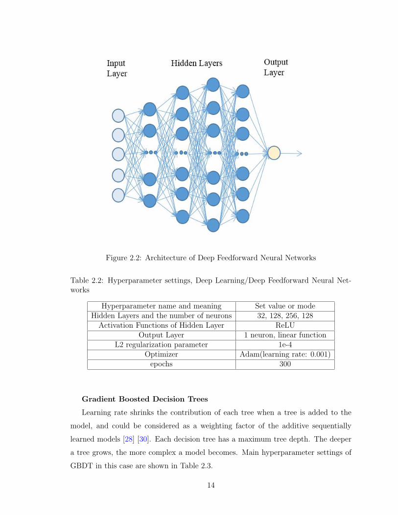
Figure 2.2: Architecture of Deep Feedforward Neural Networks
Table 2.2: Hyperparameter settings, Deep Learning/Deep Feedforward Neural Net-works
Hyperparameter name and meaning Set value or modeHidden Layers and the number of neurons 32, 128, 256, 128
Activation Functions of Hidden Layer ReLUOutput Layer 1 neuron, linear function
L2 regularization parameter 1e-4Optimizer Adam(learning rate: 0.001)
epochs 300
Gradient Boosted Decision Trees
Learning rate shrinks the contribution of each tree when a tree is added to the
model, and could be considered as a weighting factor of the additive sequentially
learned models [28] [30]. Each decision tree has a maximum tree depth. The deeper
a tree grows, the more complex a model becomes. Main hyperparameter settings of
GBDT in this case are shown in Table 2.3.
14

Table 2.3: Hyperparameter settings, GBDT
Hyperparameter name and meaning Set value or modeThe number of regression trees 250
Learning rate 0.01Maximum regression tree depth 5
Random Forest
Minimum number of samples required to be at a leaf node controls the depth of a
regression tree. While a tree is being trained, a randomly selected number of features
are considered to split an internal node. The maximum number to consider equals to
the square root of the total number of features in this setting. Main hyperparameter
settings of Random Forest in this case are shown in Table 2.4.
Table 2.4: Hyperparameter settings, Random Forest
Hyperparameter name and meaning Set value or modeThe number of regression trees in forest 500
Maximum features to The square rootconsider in each split of the number of features
Minimum number of samples 0.01× therequired to be at a leaf node number of samples
Support Vector Regression
We choose Radial Basis Function as the kernel in this case after testing different
kernel choices. Penalty parameter controls the trade-off between bias and variance.
Main hyperparameter settings of SVR in this case are shown in Table 2.5.
15

Table 2.5: Hyperparameter settings, Support Vector Regression
Hyperparameter name and meaning Set value or modeKernel function Radial Basis Function
Penalty parameter for the error 0.5term in loss function
Kernel Parameter 10Epsilon 0.1
Ridge Regression
Regularization parameter controls the bias and variance trade-off. Main hyperpa-
rameter settings of Ridge Regression in this case are shown in Table 2.6.
Table 2.6: Hyperparameter settings, Ridge Regression
Hyperparameter name and meaning Set value or modeRegularization strength parameter 2.5
Linear Regression
There is no hyperparameter in Linear Regression.
2.4.4 Software and Platform
In this work, the model developments and evaluations are performed in Python 2.7,
in Mac OS X 10.11.5 environment.
First, to develop a deep learning model, we chose Keras 2.0.6 [39], which is a widely
used open source neural network library in Python, and used TensorFlow 1.0.0 as its
backend, which is developed by Google [40].
Second, for other machine learning methods investigated in this study, such as
Random Forest, Gradient Boosted Decision Trees, Support Vector Regression, Ridge
Regression and Multiple Linear Regression, we used scikit-learn version 0.18.1 [41]
[42].
16

2.5 Results and discussions
First, we report and discuss the performance of each model on test data with the
hyperparameter settings discussed in Section 2.4.3. Next, we perform analysis on the
obtained results considering the characteristics of each algorithm. Only normalized
data results are shown for data proprietary.
2.5.1 Performance on test data
In this subsection, we show the predictive performance of each model (see Figure 2.3
to Figure 2.8). The performance statistics of different models such as MAE, MSE,
and Pearson correlation coefficient are presented in Table 2.7.
Table 2.7: Test results
Methods Test Test Pearson CorrelationMAE MSE Coefficient
Deep Learning 0.28615 0.16440 0.78320GBDT 0.22425 0.10475 0.80857
Random Forest 0.23073 0.11927 0.77248SVR 0.27219 0.17925 0.65551
Ridge Regression 0.53630 0.38927 0.26273Linear Regression 0.53633 0.38931 0.26270
17
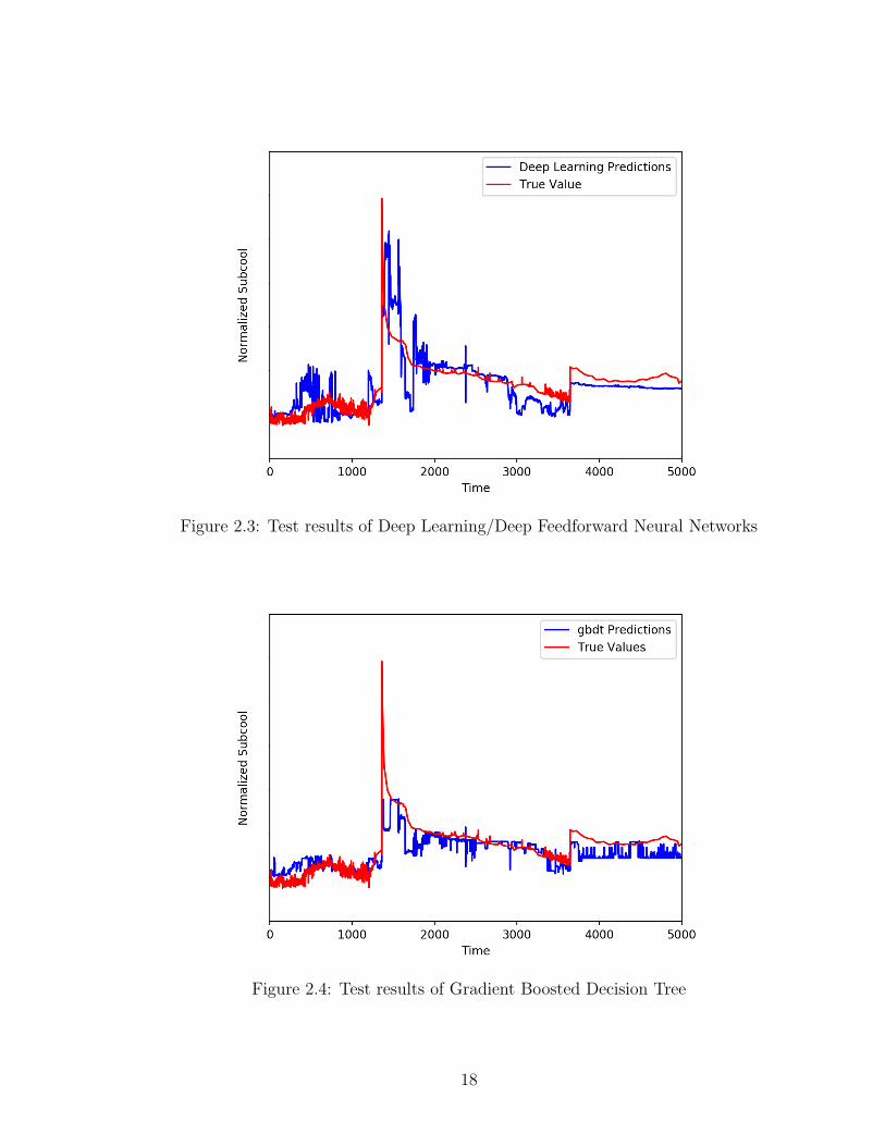
Figure 2.3: Test results of Deep Learning/Deep Feedforward Neural Networks
Figure 2.4: Test results of Gradient Boosted Decision Tree
18

Figure 2.5: Test results of Random Forest
Figure 2.6: Test results of Support Vector Regression
19
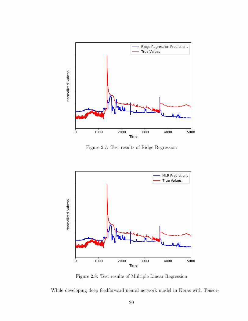
Figure 2.7: Test results of Ridge Regression
Figure 2.8: Test results of Multiple Linear Regression
While developing deep feedforward neural network model in Keras with Tensor-
20
Flow as its backend, we should note that the issue of randomness may lead to non-
reproducible results, which comes from the random initialization weights, shuffling
data, mini-batch in optimization, and implementation of tools for parallel computing
[39] [40]. Strategies to solve it vary from environments, problems and motivations. In
our case, to make full use of the power of mini-batch, we do not control randomness
of shuffling data and mini-batch in optimization. We train the model with the same
settings and data 10 times, separately. Each of the 10 models will produce a predic-
tion. All the well-trained models are saved. Thus, we report the results with the best
MAE of the 10 deep models. We apply the same strategy in Section [? ]. Statistics
of the 10 model results of test data are included in Table 2.8.
Table 2.8: Statistics of Deep Learning/Deep Feedforward Networks results of Section2.5.1
Metrics Name Minimum Maximum Mean VarianceMAE 0.28615 0.44967 0.36691 0.00343MSE 0.16339 0.35927 0.25330 0.00439
Pearson Correlation 0.70321 0.79718 0.74776 0.00112
2.5.2 Discussion
First, it is obvious that the non-linear methods have better performance compared to
linear methods due to inherent nonlinearity of the dataset. Moreover, there is a slight
improvement using the Ridge Regression compared to Multiple Linear Regression,
since Ridge Regression shrinks coefficients. Therefore, the model is underestimated
with linear methods, and a more complex model is required.
Second, it can be observed that SVR outperforms linear methods. The kernel
trick in SVR doing feature expansion not only deals with data nonlinearity, but also
implies that there are some hidden features in the process from the 5 input features
to subcool because of its better performance than linear methods. Also, we see a
relatively smoother plot in Figure 2.6. It could be explained by the threshold epsilon,
which makes the prediction less sensitive to smaller noises.
Comparison between the Random Forest and GBDT indicates that GBDT per-
forms better in terms of MAE, MSE and Pearson correlation coefficient, but both
21

methods perform well. As introduced earlier, both methods apply multiple models to
estimate the single final prediction. Random Forest applies bagging, whereas GBDT
applies boosting. This is one reason why they both perform well. Moreover, they
are both based on Regression Tree. Regression Tree is trained in a quantitative way,
so prediction is performed through comparison between the value of the correspond-
ing feature and the internal nodes. As a result, both quantitative and qualitative
relationships between subcool and selected features are influential in this case. In
addition, using the samples of the leaf node for prediction can decrease the effect of
noisy data where noise originated from environment, sensors, etc.
Deep learning method does not show the best results in terms of MAE, MSE and
Pearson correlation coefficient. However, the trend plot of the Deep Learning model
can capture the peak in the trend very well while all other models more or less failed
in capturing the peak. This is because of the flexibility of deep learning model and
powerful optimization algorithm. First, we apply multiple layers and the number of
neurons in each hidden layer can be changed. Therefore, the automatic latent feature
expansion and reduction within multiple hidden layers imply the meaningful results
of deep feedforward neural network. Second, the ReLU activation function does not
suffer from saturation problem [22]. Both of these features contribute to the flexibility
of the model. Also, a good model needs a powerful optimization algorithm to train
parameters. The Adam, a stochastic optimization algorithm, has the advantages of
bias correction and individual adaptive learning rate, which makes it useful in solv-
ing non-convex optimization problem [27]. Hence, the model flexibility and powerful
optimization algorithms make deep learning perform the best in capturing the trend.
2.6 Data quality and priori knowledge play a vital
role
In this section, we show that data quality and priori knowledge play a vital role
when using machine learning tools to solve oil sands problems. We first continue
prediction on a new dataset following the procedure described in Section 2.4. We see
that bad performance is obtained. Then, we investigate the original industrial dataset
22

and do more analysis on the results. The investigation and analysis emphasize the
importance of data quality and priori knowledge.
2.6.1 Case Study on a different dataset
In this subsection, another set of data, containing 37,100 data points after data clean-
ing, is considered. The first 25,000 data points are used as training data, while the
rest 12,100 data points are test data. Data normalization and model hyperparameter
settings are explored again and poor performance has been reported on the new test
data.
Table 2.9 to Table 2.13 show the hyperparameter settings in this dataset. As
before, those hyperparameters are explored on training data.
Table 2.9: Hyperparameter settings of new dataset, Deep Learning/Deep FeedforwardNeural Networks
Hyperparameter name and meaning Set value or modeHidden Layers and the number of neurons 32, 128, 256, 128
Activation Functions of Hidden Layer ReLUOutput Layer 1 neuron, linear function
L2 regularization parameter 1e-4Optimizer Adam(learning rate: 0.001)
epochs 300
Table 2.10: Hyperparameter settings of new dataset, GBDT
Hyperparameter name and meaning Set value or modeThe number of regression trees 400
Learning rate 0.01Maximum regression tree depth 5
23
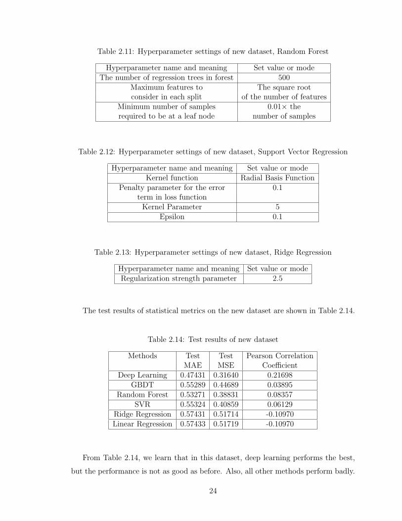
Table 2.11: Hyperparameter settings of new dataset, Random Forest
Hyperparameter name and meaning Set value or modeThe number of regression trees in forest 500
Maximum features to The square rootconsider in each split of the number of features
Minimum number of samples 0.01× therequired to be at a leaf node number of samples
Table 2.12: Hyperparameter settings of new dataset, Support Vector Regression
Hyperparameter name and meaning Set value or modeKernel function Radial Basis Function
Penalty parameter for the error 0.1term in loss function
Kernel Parameter 5Epsilon 0.1
Table 2.13: Hyperparameter settings of new dataset, Ridge Regression
Hyperparameter name and meaning Set value or modeRegularization strength parameter 2.5
The test results of statistical metrics on the new dataset are shown in Table 2.14.
Table 2.14: Test results of new dataset
Methods Test Test Pearson CorrelationMAE MSE Coefficient
Deep Learning 0.47431 0.31640 0.21698GBDT 0.55289 0.44689 0.03895
Random Forest 0.53271 0.38831 0.08357SVR 0.55324 0.40859 0.06129
Ridge Regression 0.57431 0.51714 -0.10970Linear Regression 0.57433 0.51719 -0.10970
From Table 2.14, we learn that in this dataset, deep learning performs the best,
but the performance is not as good as before. Also, all other methods perform badly.
24

Next, we show the trend plots of different tested methods. From Figure 2.9 to Figure
2.14, we also see that all of them failed to perform well. We will discuss why this
occurs in the next subsection.
Figure 2.9: Test results of Deep Learning/Deep Feedforward Neural Networks usingnew dataset
25
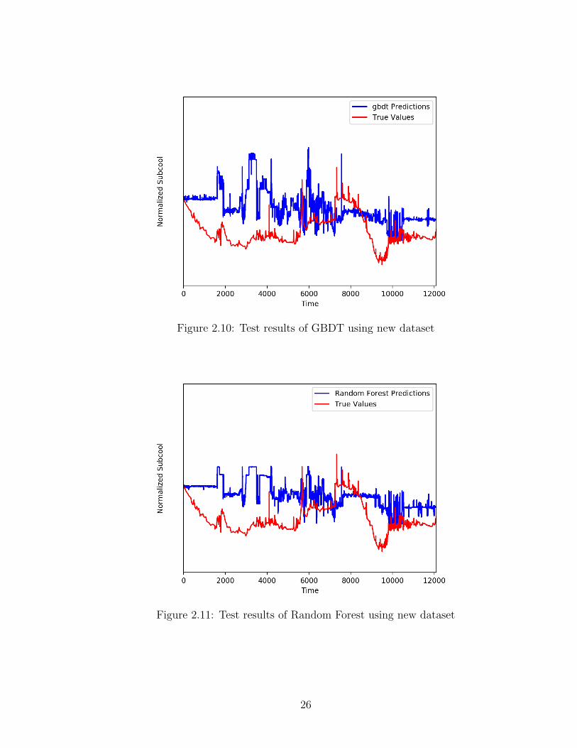
Figure 2.10: Test results of GBDT using new dataset
Figure 2.11: Test results of Random Forest using new dataset
26

Figure 2.12: Test results of Support Vector Regression using new dataset
Figure 2.13: Test results of Ridge Regression using new dataset
27

Figure 2.14: Test results of Multiple Linear Regression using new dataset
2.6.2 Investigation to original dataset and analysis
We have investigated the original data to see what occurred in the period of this set
of data. We found there were obvious operation condition changes between the range
of training data and testing data.
Because of closed-loop control and cascade control, the operational condition
changes can be reflected by several variables. See Figure 2.15 for Injection Tubing
Pressure, where training data period and testing data period is split by red dashed
line. From this figure, we can see that much more significant downtrend oscillations of
the injection tubing pressure occurred in the testing data period, than those occurred
in the training data period, and this phenomenon has invalidated the model learned
from the training data. Therefore, the data quality in engineering applications plays
a critical role in the process data analytics and machine learning. Meanwhile, priori
knowledge of the industrial process can also help in dealing with this type of prob-
lems.
28
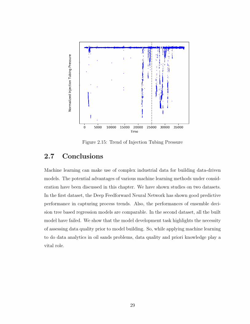
Figure 2.15: Trend of Injection Tubing Pressure
2.7 Conclusions
Machine learning can make use of complex industrial data for building data-driven
models. The potential advantages of various machine learning methods under consid-
eration have been discussed in this chapter. We have shown studies on two datasets.
In the first dataset, the Deep Feedforward Neural Network has shown good predictive
performance in capturing process trends. Also, the performances of ensemble deci-
sion tree based regression models are comparable. In the second dataset, all the built
model have failed. We show that the model development task highlights the necessity
of assessing data quality prior to model building. So, while applying machine learning
to do data analytics in oil sands problems, data quality and priori knowledge play a
vital role.
29

Chapter 3
Locally Weighted QuadraticRegression based BayesianOptimization and its application inSAGD process
This chapter proposes the Locally Weighted Quadratic Regression based Bayesian
Optimization (LWQRBO) method. This optimization algorithm inherits the Bayesian
Optimization algorithm framework with Expected Improvement as the figure of merit
for search. It utilizes locally weighted quadratic regression as the surrogate model.
Further, the proposed LWQRBO is applied in a simulated SAGD process.
This chapter is organized as follows: Section 3.1 presents the brief review of lit-
erature on Bayesian Optimization. Section 3.2 revisits Efficient Global Optimiza-
tion (EGO) and Locally Weighted Learning (LWL), and then proposes the Locally
Weighted Quadratic Regression based Bayesian Optimization (LWQRBO). Next, two
numerical cases are studied to test the proposed LWQRBO in Section 3.3. SAGD
optimization literature review, problem description and the application of LWQRBO
in SAGD process are discussed in Section 3.4. Conclusions are drawn in Section 3.5.
3.1 Literature Review of Bayesian Optimization
Derivative-free optimization (DFO) is of great importance in practical applications,
and is necessary when the derivatives of the objective function are not available or
30

hard to compute, such as in the cases where the objective function is a computer simu-
lation, a physical process or a complex mathematical function. DFO includes various
classes of algorithms. For example, trust-region methods and Nelder-Mead simplex
algorithm belong to local search methods, and multilevel coordinate search, branch-
and-bound search and Response Surface methods belong to global search methods
[43]. The well-known Mesh Adaptive Direct Search (MADS) is an extension of Gen-
eralized Pattern Search method [44], which also belongs to DFO. In this chapter,
we are particularly interested in one of the subjects of DFO, Bayesian Optimization,
which deals with optimizing black-box objective functions.
Jones et al. [45] proposed an Efficient Global Optimization (EGO) algorithm,
which aims to optimize the black-box objective function by building the stochastic
process response surface. Expected Improvement (EI) is used as the figure of merit
which accounts for both the approximate function, and uncertainty of the surface.
Maximization of EI yields a next sample point which is a trade-off solution to local
and global search. Branch-and-bound algorithm is used to solve the sub-optimization
problem - maximizing Expected Improvement. Gramacy et al. [46] proposed an
algorithm to solve the optimization problem with black-box objective function and
black-box constraints. To this end, the Augmented Lagrangian methods are applied
to convert a constrained problem into an unconstrained problem, and the algorithm
is integrated with Gaussian Process surrogate modelling, Expected Improvement and
derivative-free methods [46]. Picheny et al. [47] included slack variables into Bayesian
Optimization with the Augmented Lagrangian Framework, and also, the introduced
slack variables are deployed to handle mixed constraints of equality and inequality,
where they are treated as “joint” black-box.
There exist several variants of the EGO algorithm. Bootstrapped EI is proposed to
estimate the variance of kriging model instead of classic EI in [48]. Further, multiple
surrogate models are adapted into the EGO framework in [49]. In this work, at each
optimization iteration, multiple sample points are obtained by maximizing EI for each
of the surrogate models, rather than a single point from a single surrogate model.
In terms of application, Bayesian Optimization was proposed as a way to tune ma-
chine learning hyperparameters in [50]. Bayesian Optimization is related to surrogate
model based black-box optimization.
31

Vu et al. [51] did a survey on surrogate model based black-box optimization.
The work discusses multiple types of surrogate models, along with different merit
functions and experiment designs. Also, entropy search is applied in Efficient Global
Optimization in [52].
Talgorn et al. [53] applied locally weighted scatterplot smoothing for constructing
a surrogate model, and therefore, to generate possible solutions. In their work, Mesh
Adaptive Direct Search (MADS) is used to solve the black-box optimization problem
with the built model. Also, the calculated shape parameter of weight function is
selected by minimizing order error. Conn and Digabel combined MADS and quadratic
models for black-box optimization [54]: The quadratic models are embedded into the
MADS, and search and ordering strategies are performed with the models used in
their work.
Dang approached the parameter tuning problem by considering it as a black-
box optimization problem, and proposed an Optimization of Algorithms (OPAL)
framework in [55]. This work also parallelized the OPAL framework and released a
Python implementation.
An overview of existing surrogate model methods and the optimization frame-
work, is given in [56], and also the usefulness of surrogate model based optimization
for certain aerodynamic problem has been shown in [56]. The work by Koziel and
Leifsson [57] includes an array of engineering applications of surrogate model based
optimization. Furthermore, Mack et al. [58] applied the surrogate model optimiza-
tion in an aerospace design problem.
3.2 Locally Weighted Quadratic Regression based
Bayesian Optimization
The Locally Weighted Quadratic Regression based Bayesian Optimization (LWQR-
BO) algorithm is proposed in this section. Prior to introducing LWQRBO, we describe
its framework, the Efficient Global Optimization algorithm, in subsection 3.2.1. The
surrogate modelling approach that is applied in this chapter, namely locally weighted
learning, is introduced in subsection 3.2.2. Next, the proposed algorithm is described
32

in detail in subsection 3.2.3.
3.2.1 Efficient Global Optimization
As discussed in Section 3.1, Bayesian Optimization includes a wide range of algo-
rithms. We introduce its basic ideas and one of its representatives, the Efficient
Global Optimization (EGO) which is proposed by Jones et al. [45]. We illustrate the
sampling process in a one-dimensional case, by introducing a normal sample strategy
followed by the sample strategy of Efficient Global Optimization. The introduction
in this subsection is referenced from [45].
(a) Initial dataset and initially built surface
(b) Dataset and built surface in one iteration
The green points represent initial points sampled from the true curve, and the purple pointdenotes the calculated sampled point. The red dashed curve represents the built surface or the
built surrogate model, and the green curve denotes the true function curve.
Figure 3.1: Sampling without considering model uncertainties
The first step is to build an initial surface with the initial dataset, and the initially
built surface is represented by the red dashed line in Figure 3.1a. Then, the sample
33

point for the next iteration is calculated. Normally, the next sample point is calculated
at the point, where it is the minimum of the initially built surface or the surface built
in the previous iteration. In Figure 3.1b, purple dot indicates the sample point for
next iteration. Next, this purple point is sampled from the true function, and the
dataset is updated by adding the newly sampled point. Furthermore, surface is built
with the new dataset, and is denoted by the red dashed line in Figure 3.1b. Finally,
iterate until the stopping criteria is met.
However, we see from Figure 3.2 that there are model uncertainties, especially
where the data are sparse. The black dashed lines represent the range of the uncer-
tainties of the model.
Figure 3.2: Model uncertainties
Bayesian Optimization considers the model uncertainties. There are many ways
to consider model uncertainties, that is, many merit functions could be applied to
determine the next sample point [50] [51]. Expected Improvement is one of them.
Following the work by Jones et al. [45], Improvement and Expected Improvement
can be defined as follows:
I(x) = max(fmin − Y, 0) (3.1)
E[I(x)] = E[max(fmin − Y, 0)] (3.2)
where fmin is the current minimum function value, and Y is the random variable to
be minimized. A more specific expression of Expected Improvement is expressed in
34

Equation 3.3 [45]:
EI(x) = (fmin − y)Φ(fmin − y
s) + sφ(
fmin − ys
) (3.3)
where fmin is minimum function value. φ(.) and Φ(.) are the standard normal density
and distribution functions, respectively. y and s denote the prediction and standard
error of prediction, respectively. From Equation 3.3, it can be seen that Expected
Improvement considers not only model uncertainty but also information of the current
minimum value and the built surface.
Efficient Global Optimization optimizes Expected Improvement to determine the
next sample point. It normally applies branch-and-bound algorithm to maximize the
Expected Improvement. It bounds the mean squared error via convex relaxation and
bounds the prediction via nonconvex relaxation [45]. However, in this work, we use
Genetic Algorithm to solve this problem, and the details of this will be presented in
subsequent sections.
3.2.2 Locally Weighted Learning
Online prediction is required in industrial processes [59]; particularly, the online pre-
dictions of quality variables are important for monitoring, control and optimization
of industrial processes. Considering that the process operation condition is changing,
the predictive model should be updated [60]. Locally Weighted Learning (LWL) is
one of the choices to build predictive models, and has been widely studied on its ap-
plication in industrial process [59] [61]. Ge and Song [60] did a comparative study of
locally weighted learning with SVR and PLS. The Locally Weighted Principal Com-
ponent Analysis associated approaches are studied in [59] [62]. Also, locally weighted
learning can handle missing data in industrial process [61]. A typical procedure of
locally weighted learning can be summarized as follows [60] [63]:
1. A query point, q, comes;
2. Distance is calculated between the query point q and each point in the historical
dataset;
3. Weight matrix of historical dataset is calculated via a weight function;
4. Do prediction with weighted dataset via a selected regression technique;
5. The built model is discarded. The system waits for the next query point.
35

Figure 3.3: Illustration of locally weighted learning
In Figure 3.3, we illustrate the idea of locally weighted learning in a one-dimensional
case. In this figure, the black points represent historical dataset, the red point de-
notes query point. The red line represents weights. It should be noted that if the
data sample lies closer to the query point, it has larger weight. In other words, LWL
selects the most relevant data to do regression, and the model is updated for each
query point. Thus, it is useful in practice for chemical processes to account for the
changing process operation conditions. Also, the locally weighted model can deal
with nonlinearity [63]. Therefore, locally weighted regression is applied as the sur-
rogate model in the Bayesian Optimization framework. Specifically, locally weighted
quadratic regression is considered.
Next, we introduce Equation 3.4 and Equation 3.5, from [63]. These equations
are related to least squares algorithms of locally weighted linear models. Equation
3.4 is the prediction expression at the point q of local linear models, and Equation
3.5 is the variance of the prediction at q of local linear models.
y(q) = qT (ZTZ + Λ)−1ZTWy
= STq y
=N∑i=1
si(q)yi (3.4)
where q is the point we want to predict, Z = WX and W denotes weight matrix. X
and y denote inputs and output of the dataset, respectively. Λ is a diagonal matrix
36

with small positive diagonal elements to avoid singular matrix.
V ar(y(q)) =∑i
s2i (q)σ2(xi) (3.5)
where si(q) comes from Equation 3.4 and σ(xi) denotes the standard deviation of
random noise at point i. The above two equations will be modified to be incorporated
into Expected Improvement. The details will be introduced in next section.
3.2.3 Locally Weighted Quadratic Regression based BayesianOptimization
First, the prediction expression of locally weighted quadratic regression must be ob-
tained. The quadratic terms in quadratic regression could be regarded as regres-
sors of linear regression. Consider a two-dimensional case. For other dimensions,
it can be modified accordingly. The inputs, Xinput = [X1, X2], are expanded to
X = [X1, X2, X21 , X
22 , X1X2] as the regressors to perform quadratic regression. X will
be weighted to Z by Z = WX. Z will be used in the general locally weighted linear
regression expression in Equation 3.4. Also, considering that solving the inverse of a
matrix may suffer from the singular matrix problem, we choose stable numerical al-
gorithms to solve the inverse of a matrix, and therefore, we set the diagonal elements
in Λ matrix to zero. So, the prediction at point q using locally weighted quadratic
regression is:
y(q) = qT (ZTZ)−1ZTWy
= STq y
=N∑i=1
si(q)yi (3.6)
As noted previously, Expected Improvement relies on prediction and standard
error of the prediction. Besides the prediction term, we also need the standard error
of prediction. For simplicity, we start the analysis without considering the random
noise. For this case, Equation 3.5 can be expressed as:
V ar(y(q)) =∑i
s2i (q) (3.7)
37

Therefore, from Equation 3.6 and Equation 3.7, the variance of prediction at point
q of the locally weighted quadratic regression can be rewritten as:
V ar(y(q)) =∑i
s2i (q)
= STq Sq
= qT (ZTZ)−1ZTW (qT (ZTZ)−1ZTW )T
= qT (ZTZ)−1ZTWW TZ(ZTZ)−1q (3.8)
Also, the standard error at the point of q of a locally weighted quadratic regression
is expressed in Equation 3.9:
std(y(q)) =√V ar(y(q))
=√qT (ZTZ)−1ZTWW TZ(ZTZ)−1q (3.9)
where X = [X1, X2, X21 , X
22 , X1X2], Z = WX, and W = fw(X, q). There are many
ways to choose the weight function, fw, and the distance, d. We choose the exponential
function as the weight function and Euclidean distance as the distance measure.
Mathematically, they are defined as [63]:
fw = ke−d/l (3.10)
where d is Euclidean distance, k and l are function parameters. The distance between
xq and xi is:
d =√
(xq − xi)T (xq − xi) (3.11)
This proposed LWQRBO algorithm solves optimization problems whose objective
function is a black-box function, with bound constraints on the decision variables. We
consider solving a minimization problem. We first introduce the steps of LWQRBO,
which inherits the framework of Efficient Global Optimization from [45]. We use a
1-d case with 3 initial points to describe it:
Steps:
1. Provide initial points (x1, x2, x3) for the optimization algorithm, and sample
from the true black-box function to calculate (y1, y2, y3).
2. Build surrogate model fs, with locally weighted quadratic regression, on the
initial dataset [(x1, y1), (x2, y2), (x3, y3)]. ymin = min(y1, y2, y3), assume xmin = x3.
38

3. Calculate the prediction y, and the standard error of prediction std, of the
built surrogate model (i.e., locally weighted quadratic regression model), at the query
point q.
4. Maximize the Expected Improvement to find the next point to sample, x4.
5. If y4 is less than ymin, set ymin = y4 and xmin = x4; Otherwise, retain
ymin and xmin; Then, update the dataset by appending new sample point and get
[(x1, y1), (x2, y2), (x3, y3), (x4, y4)].
6. If stopping criteria are met, (i.e., EI satisfying the prescribed threshold value,
or the maximum number of iterations reached), the algorithm stops. The solution is
xmin, with the objective function value ymin. Otherwise, repeat Step 2 to Step 6 with
the appended dataset.
Now, let us see the specific details of the proposed algorithm, LWQRBO. In this
work, to use locally weighted quadratic regression as the surrogate model, suitable
modifications are made to the EGO framework. Analysis and explanation are also
described for applying locally weighted quadratic regression in this framework. Spe-
cific details of the algorithm are as follows:
Providing Initial Dataset
Latin hypercube sampling is applied to provide the initial points [45], and the num-
ber of sampled points is around 10p, where p is the dimension of the function inputs,
or variables of the surrogate model [45]. p is also the number of decision variables of
the optimization algorithm. After sampling from the true black-box function with ini-
tial points to obtain corresponding outputs, the initial dataset have been constructed.
Preparing for Expected Improvement
Calculate the prediction y(q) with Equation 3.6, and the standard error of pre-
diction std(q) with Equation 3.9, at the new point q, or called query point, with
locally weighted quadratic regression. These are used for the calculation of Expected
Improvement.
Calculating Expected Improvement
Calculate Expected Improvement, by replacing y and s in Equation 3.3, with E-
39

quation 3.6 and Equation 3.9, respectively. The estimation of Expected Improvement
at point q of a locally weighted quadratic regression could be written as:
EI(q) = (fmin − qT (ZTZ)−1ZTWy)Φ(fmin − qT (ZTZ)−1ZTWy√
qT (ZTZ)−1ZTWW TZ(ZTZ)−1q)
+(√qT (ZTZ)−1ZTWW TZ(ZTZ)−1q)φ(
fmin − qT (ZTZ)−1ZTWy√qT (ZTZ)−1ZTWW TZ(ZTZ)−1q
)
(3.12)
where fmin is the current best function value. φ(.) and Φ(.) are the standard normal
density and distribution functions, respectively. X and y denote input and output,
respectively. q is the unknown point or query point. W is weight matrix calculated
by weight function shown in Equation 3.10. Z is the weighted matrix of X.
Maximizing EI
In Step 4, we want to maximize EI(q) to find the next sample point. It is a
sub-optimization problem, and we provide a description of the solution below.
First, it consists of probability density and distribution function. Second, we
consider it in view of modelling: Assume we have training data and testing data, and
will make predictions for all the inputs in testing data. Locally weighted learning
has different model parameters for different inputs of testing data, with the same
training data. Because it builds a model for each input in test data, implying W
and Z in Equation 3.12 could be different for different data points to be predicted.
Additionally, W and Z are unknown, and are functions of q.
Equation 3.12 is therefore a highly non-linear and complex function with respect
to q, and is hardly tractable analytically. Hence, Genetic Algorithm is applied to
solve this sub-optimization problem.
Stopping Criteria
If the stopping criteria are not met, the dataset is updated by adding the obtained
query point q and its function value, yq, sampled from the true black-box function.
Then, we use locally weighted quadratic regression in next iteration with the updated
dataset to build the model. Otherwise, it stops. The stopping criteria is controlled
by the following:
1. If the Expected Improvement is less than a specified percentage, p1, of the
40

current minimum value fmin, it stops;
2. If the new sampled objective function value is less than a specified percentage,
p2, of the current minimum value, it stops;
3. If the number of iterations, or black-box calculations exceeds maximum calcu-
lations M , it stops.
All of the above stopping criteria could be used in the algorithm. The mode of
each criterion can be adjusted accordingly in practice. Criteria 1 and 2 allow the
optimization algorithm to explore more of the optimum and Criterion 3 controls the
calculation time.
Figure 3.4 presents the flowchart of the proposed approach. The main modifica-
tions in the existing framework are highlighted in boldface.
41

Figure 3.4: Flowchart of LWQRBO
3.3 Case Study
In this section, we present the validation results of Locally Weighted Quadratic Re-
gression based Bayesian Optimization (LWQRBO) in two numerical test functions.
42

3.3.1 Case Study 1
In this subsection, we apply the Bayesian Optimization with locally weighted quadrat-
ic regression algorithm in a one-dimensional numerical test function, as given in E-
quation 3.13:
y =x
10sin(
π
2x) (3.13)
where x ∈ [1, 10].
Figure 3.5 shows the true curve of this test function as the black line. It has one
global minimum and several local minima. Latin hypercube sampling is applied to
sample the 10 initial data points, which are marked in the figure by blue markers.
The initial data points are distributed across the range [1, 10] almost evenly. Red
points represent the sampled points calculated by the optimization algorithm. We
see that most of the sampled points are clustered around the global minimum.
Figure 3.5: Curve of 1-d test function
43

Figure 3.6 shows the performance of optimization algorithm through iterations.
The red line represents the sampled function value and blue line represents the current
calculated minimum, also called the best calculated value until the current iteration.
We see that the blue line gradually converges to the global minimum.
The algorithm samples where the Expected Improvement is maximized. As dis-
cussed before, Expected Improvement takes both model uncertainty and optimization
into consideration. It is not necessary that the function value of the sampled point in
next iteration is lower than that in the current iteration. Because the sampled points
not only consider exploring the minimum in next iteration but also consider model
uncertainty to make the built surface more accurate. The current minimum value
is updated during the iterations in the optimization algorithm, and therefore keeps
decreasing.
Figure 3.6: Performance through iterations
44

The dashed vertical line marks a separation between the initial dataset and newly
found sample points as the optimization process progressed. It shows that the min-
imum finally found is not the minimum in initial dataset, which also demonstrates
this sampling algorithm indeed works.
Expected Improvement is maximized at each iteration to determine the next sam-
ple point. Figure 3.7 shows iterative trend of the Expected Improvement.
Figure 3.7: Expected Improvement of 1-d case
45

3.3.2 Case Study 2
The proposed algorithm is also tested in a 2-dimensional numerical function, called
Branin function.
The Branin function is expressed in Equation 3.14 [64]:
y = a(x2 − bx21 + cx1 − r)2 + s(1− t)cos(x1) + s (3.14)
where we choose the following settings:
a = 1, b = 5.14π2 , c = 5
π, r = 6, s = 10 and t = 1
8π. x1 ∈ [−5, 10] and x2 ∈ [0, 15].
For those settings, the function has 3 global minima:
The function value is f(x∗) = 0.397887, at x∗ = (−π, 12.275), (π, 2.275) and
(9.42478, 2.475) [64].
Figure 3.8: Locations of sampled points
46

Figure 3.8 shows locations of the sampled points. The 21 initial data points
are distributed in the square range and are denoted by blue markers. Three green
triangles represent locations of the three global optima. Red points represent the
points obtained by maximizing EI. We see that most points sampled during iterations
are around two of the three global optima, x∗ = (−π, 12.275) and (9.42478, 2.475).
Figure 3.9 illustrates the performance of LWQRBO on the Branin test function. As
discussed before, we know the function value of the sampled points during iterations
are regarded as candidates of the final optima, since maximizing EI considers the
trade-off between surface optima exploitation and consideration of model uncertainty.
Therefore, the algorithm does not guarantee its continuous decrease. Moreover, we
see that the current calculated minimum (blue line) converges to global optimum
gradually, from 0.3985, 0.3983 to 0.3981. The obtained optimal point is located at
(−3.1477, 12.2983), which is very close to (−π, 12.275), as seen in Figure 3.8.
Figure 3.9: Performance through iterations
Points to the left of the vertical line are the initial dataset, and those to the right
are the points determined as the optimization process progressed. The vertical axis
47

is log scaled for the purpose of a clear view; otherwise, the curve decreases quickly
and steeply in linear scale.
Expected Improvement is maximized to calculate the next sample point. Figure
3.10 shows the trend of Expected Improvement through iterations.
Figure 3.10: Expected Improvement of 2-d case
3.4 Application in simulated SAGD process
In this section, Locally Weighted Quadratic Regression based Bayesian Optimization
(LWQRBO) is applied to a simulated SAGD process. In subsection 3.4.1, a literature
review of SAGD optimization is provided. The motivation and description of the
problem are formulated in subsection 3.4.2. In subsection 3.4.3, optimization results
are presented.
48

3.4.1 SAGD Optimization Review
SAGD is an efficient approach to extract bitumen from reservoir from an economic
point of view [65], and it has been extensively used to produce bitumen, especially in
Alberta, Canada. The optimization solutions of SAGD can help engineers with the
decision-making process [66].
SAGD production can be enhanced with first principle knowledge and therefore,
there are many variants [67]. One approach to improve SAGD is to design the injected
steam. Two well-known variants of this type are Steam and Gas Push (SAGP),
and Expanding Solvent SAGD (ES-SAGD) [67] [68]. SAGP injects steam with non-
condensed gas, such as nitrogen or natural gas; ES-SAGD injects steam with solvent
[68]. Also, an elaborate design of the SAGD facilities, especially the well design,
improves SAGD efficiency. The effect of well design, such as lengths, liner and tubing,
wellbore annulus on SAGD performance has been discussed in [69]. Furthermore, in
the cases where reservoirs are very thin, one-well SAGD [67] could be considered as
a candidate.
Steam injection strategy plays an essential role in SAGD optimization. Optimizing
SAGD by adjusting steam injection pressure with a reservoir simulation model is
studied in the work by Card et al. [5]. In the study by Gates et al. [70], optimization
is also performed by adjusting injection pressure. Also, the role of steam injection
strategy in determining the performance of SAGD is described in [71] and [72].
Optimizing economic performance of SAGD is a main focus. There are many
economic performance measurements of the SAGD process, such as Steam to Oil
Ratio (SOR), cumulative Steam to Oil Ratio (cSOR), Net Present Value (NPV),
etc. The economic performance measurement to use depends on the problem being
investigated. For example, the work of [70] studies optimization of cSOR via Genetic
Algorithm, and Net Present Value (NPV) is considered as an objective to be optimized
in [71]. Other economic performance measurements, such as Internal Rate of Return
(IRR) and Pay Back Period (PBP) are studied in [65].
Uncertainty is another research topic while doing optimization in SAGD. The
study in [71] considers the uncertainty of the economic forecast when optimizing
the SAGD process, and Monte Carlo simulation is used to quantify uncertainty in
49

this work. Uncertainty also arises from reservoir geological properties. In [73], a
SAGD optimization workflow is presented to capture the geological uncertainties.
Another study [74] proposes to reduce reservoir geological property uncertainties using
a mixed-integer linear optimization-based method.
Surrogate model based optimization in SAGD also receives a variety of research
focuses. Work by Mohaghegh et al. [4] introduces the development of Surrogate
Reservoir Modelling. In [75], Polynomial model and Kriging model are constructed
as proxy models, then the gradient based algorithm is applied for optimization. Yang
et al. [71] have built polynomial response surface for NPV to perform an economic
optimization of SAGD. Besides, Network-based efficient global optimization (NEGO)
method is applied to optimize the SAGD process in [76].
We learn from the above review that SAGD optimization could be conducted using
various methods. Readers are referred to [3] for more information. This section aims
to optimize the SAGD process. More details are introduced in the next subsections.
3.4.2 Motivation and Problem Description
To optimize SAGD, we need to build an optimization model. An optimization model
consists of three main elements: objective function, decision variables and constraints.
We introduce and discuss each element in detail below.
From Section 3.4.1, we know that there are many metrics measuring the perfor-
mance of SAGD process, such as Steam to Oil Ratio (SOR), cumulative Steam to Oil
Ratio (cSOR), Net Present Value (NPV), etc. In this study, SOR is utilized as the
objective function to be optimized.
50

Figure 3.11: Schematic of SAGD process
Figure 3.11 shows a schematic of the SAGD process. We see that the produced
liquid consists of oil and water. SOR is calculated as the ratio of the injected steam
flowrate to the produced oil flowrate, as follows:
SOR =Flowrate of Injected Steam
Flowrate of Produced Oil(3.15)
From Equation 3.15, we know that a smaller value of SOR means more produced
oil with less injected steam, while a larger SOR value means more injected steam
with less produced oil. To optimize the SAGD process performance measured by
SOR, we need to minimize SOR. However, the mathematical function describing the
relationship between SOR and other process variables is not available. Therefore, we
regard the objective function as a black-box function.
Also, from [5], [70], [71] and [72], it is learned that steam injection strategy plays
a core role in the performance of SAGD process. Thus, we focus on optimizing SOR
by determining the optimal injected steam operating point. Specifically, flowrate and
pressure of the injected steam are regarded as decision variables. They are operational
variables, and could be manipulated or controlled in practice according to the feasible
solution of the optimization model.
Those manipulated variables have operational ranges in practice for the purpose
of safety, and those upper and lower bounds of the process variables are constraints
in this optimization problem.
51
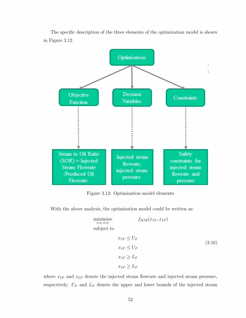
The specific description of the three elements of the optimization model is shown
in Figure 3.12.
Figure 3.12: Optimization model elements
With the above analysis, the optimization model could be written as:
minimizexIF ,xIP
fSOR(xIF , xIP )
subject to
xIF ≤ UF
xIP ≤ UP
xIF ≥ LF
xIP ≥ LP
(3.16)
where xIF and xIP denote the injected steam flowrate and injected steam pressure,
respectively. UF and LF denote the upper and lower bounds of the injected steam
52

flowrate, separately. UP and LP denote the upper and lower bounds of injected steam
pressure, separately.
The purpose is to identify an optimal operation condition, which will generate the
corresponding optimal SOR of the SAGD process. The proposed LWQRBO algorithm
in this chapter is applied to solve this optimization problem.
In LWQRBO, maximizing EI is utilized to find the point which is able to improve
the objective function value most probably, with the uncertainties in the surrogate
model being considered. The surrogate model constructed here is an approximation
of the black-box function (a real process in this work) that we want to learn. If the
relationship between inputs and output changes over time, EI cannot capture the
uncertainties in the surrogate model, which models the black-box objective function.
We therefore target this case in SAGD process: the function of SOR with respect
to injection flowrate and injection pressure is static. That is, if given the same inputs
(injected flowrate and pressure), the process will respond and generate the same SOR.
In this case, other variables of SAGD may contain dynamic relationships, but the
static relationship between SOR and injection flowrate as well as injection pressure
holds. In this period, the black-box function to be optimized is a static time-invariant
function, and therefore, we could apply LWQRBO to sample from the real process.
Considering the optimization algorithm to sample from real process, we see the
following difference from sampling from a numerical function:
1. Historical dataset plays the role of initial points.
2. Sampling a real process at different time instances plays the role of different
iterations in the optimization algorithm.
3.4.3 Optimization Results
In this subsection, we show the SAGD optimization results obtained using the L-
WQRBO method. Some of the main parameters of the reservoir are listed in Table
3.1.
Table 3.2 lists the operational upper and lower bounds of the injection flowrate
and injection pressure in this case study.
Figure 3.13 shows the procedure of the optimization algorithm. 21 historical
data points are provided as initial data in this problem. After building the initial
53

Table 3.1: Reservoir Parameters
Parameter Name ValueWell length (m) 250
Heat transfer coefficient of the liquid pool (W/m2/K) 0.5 ∗ 106
Latent heat of steam vaporization (J/kg) 780 ∗ 103
Reservoir temperature (◦C) 4Thermal diffusivity of reservoir (m2/s) 6.4467 ∗ 10−7
Porosity of formation 0.35Oil saturation 0.85Steam quality 0.95
Table 3.2: Operational Bounded Constraints
Parameter Name ValueUpper Bound of Injection Flowrate (lb/s) 7Lower Bound of Injection Flowrate (lb/s) 1Upper Bound of Injection Pressure (psi) 2200Lower Bound of Injection Pressure (psi) 1500
surrogate model, the sampled point in next iteration is found by maximizing Expected
Improvement. The red line represents the sampled function value (real value of SOR
with respect to the sampled input), which is generated from the real process, and the
blue line represents the optimal value obtained up to the current iteration. Every
time the algorithm samples from the process, the dataset is updated.
54

Figure 3.13: SAGD Optimization performance
As discussed in Section 3.3, the sampled points of input are just candidate solu-
tions for the optimal value, and the sampled function value does not need to be less
than that in the previous iteration. The blue line shows that the current minimum
decreases during the iterations of the optimization algorithm.
All iterations shown above in Figure 3.13 solve one optimization problem. The
optimization algorithm ends after the 50th iteration and the optimal SOR is found as
2.358. The corresponding input, the injection flowrate being 1 lb/s and the injection
pressure being 1500 psi, will be implemented in the real process. Figure 3.14 shows
the trend of Expected Improvement iteratively.
55

Figure 3.14: Trend of Expected Improvement
Figure 3.15 shows the location of initial data points and the sampled data points
within the given operational region. Initial data points are denoted by the circles.
The solid points represent the sampled points in the optimization algorithm, and
are located both inside the region and along the edges. It demonstrates that the
optimization algorithm does not search in a local neighborhood only. Instead, it also
samples where the data are more sparse and where the model is more uncertain, which
can be observed from the lower region of the left edge and the upper region of the
right edge. Finally, it locates the optimum at (1, 1500), which is the lower left corner.
56

Figure 3.15: Location of Initial Data and Sampled Data
3.5 Conclusions
In this chapter, Locally Weighted Quadratic Regression based Bayesian Optimization
(LWQRBO) is proposed. The literature review includes Bayesian Optimization and
related research subjects, such as Derivative-free Optimization and Surrogate Model
based Black-box Optimization. Efficient Global Optimization and Locally Weighted
Learning are introduced prior to the introduction of the proposed approach for mak-
ing the procedures of LWQRBO easy to understand. Two numerical test functions
are applied to test the performance of the proposed approach. LWQRBO is also
applied in a simulated SAGD process to optimize SOR by determining the optimal
injection steam operational points. The proposed LWQRBO algorithm demonstrates
its usefulness in SAGD process.
57

Chapter 4
Stacking online soft sensorapplication in SAGD process
In this chapter, a stacking online soft sensor that is applicable for monitoring pur-
poses is designed for the SAGD process. The literature review of soft sensor design
approaches is included in Section 4.1. The proposed online soft sensor approach is in-
spired by stacking models, so a brief review of stacking models is included in Section
4.2. Next, three popular models in soft sensor applications, Partial Least Squares
Regression (PLSR), Gaussian Process Regression (GPR) and Support Vector Regres-
sion (SVR), are introduced in Section 4.3 and they are applied as offline predictive
models. In Section 4.4, the proposed stacking online soft sensor and its feasibility are
described in detail. Two case studies are shown in Section 4.5. Conclusions to this
chapter are provided in Section 4.6.
4.1 Review of soft sensor design approaches
Soft sensors are useful in the monitoring of industrial processes [77] [78] [79]. For ex-
ample, they are applied to predict the process variables which are difficult to measure
online, such as the water content of the produced liquid of SAGD process. They are
also alternatives to expensive hardware sensors [77]. Moreover, hardware sensors are
not always available due to sensor maintenance or replacement, and soft sensors can
be utilized as a backup [77]. In most chemical engineering applications, the process
is time varying, multi-modal and nonlinear [77]. Therefore, it is necessary to improve
58

soft sensors to make them applicable for online prediction or model updates.
Many strategies have been applied to design soft sensor models. Ensemble learn-
ing is one of them. Kaneko and Funatsu developed Support Vector Regression (SVR)
based adaptive soft sensor with Bayesian ensemble learning in [80]. In their work, pre-
dictions were first made with Online Support Vector Regression (OSVR), and these
predictions were combined through Bayesian ensemble learning to obtain a final pre-
diction. In the work by Kaneko and Funatsu [81], a final prediction is obtained by
ensembling multiple predicted values from multiple intervals of time difference. An-
other adaptation mechanism for online prediction using soft sensors was proposed in
[79]: Input variables selection is performed with mutual information. The selected
variables are then used for prediction with a mixture of Gaussian Process Regres-
sion (GPR) models. Adaptation of combination weights and local GPR models are
considered for a final prediction.
Besides ensemble learning, local learning frameworks have been used for soft sen-
sor applications [82]. Kadlec and Gabrys proposed Incremental Local Learning Soft
Sensing Algorithm (ILLSA) [82], where adaptations such as recursive adaptation of
models and adaptation of combination weights could be performed. Also, another
work by Kadlec and Gabrys [83] applies local learning to build online predictive mod-
els for the consideration of noise, drifting data and outliers. In this study, input space
is partitioned to build several local models, and then predictions of different models
are combined to obtain the final prediction.
We have introduced the design of soft sensors in terms of frameworks or strategies.
The framework needs specific modelling approaches. Therefore, we also review soft
sensor applications briefly from a modelling perspective. We have seen that Gaussian
Process Regression has been used as soft sensors in [79]. Support Vector Regression
(SVR) is another common choice for predictive modelling in chemical soft sensor
applications. Bayesian approaches could ensemble SVR based models for a soft sensor
development [80]. In [78], the author proposed a soft sensor framework, incorporating
Bayesian Inference and SVR models to deal with measurement uncertainties, such as
biases and misalignments. In this work, Bayesian Inference is applied first to process
input measurements. The processed inputs are then used for two-stage SVR models.
The second stage SVR serves as the main model to make predictions [78]. Besides
59

Gaussian Process Regression and Support Vector Regression, Partial Least Squares
Regression is also a commonly used method in chemical process for soft sensing.
Partial Least Squares Regression was applied for soft sensing in a refining process
in petrochemical industry by Wang et al. [84], and in their work, PLS regression
was enhanced to handle the dynamics of the process. Additionally, Shao and Tian
built an adaptive soft sensor with local PLS models and Bayesian inference for model
ensembles [85].
Based on the literature reviewed above, it can be deduced that there are multiple
design approaches in soft sensing application, each of which have been proved to be
useful. For example, the adaptiveness of soft sensors could use the advantages of dif-
ferent models, handle online outliers and uncertainties, as well as improve prediction
accuracy. Also, most soft sensor designs focus on online applications. In this section,
the studies of different soft sensor design approaches and algorithms are briefly intro-
duced. In the next section, a novel idea will be introduced as the foundation for our
proposed stacking soft sensor, which is based on stacking multiple predictive models.
4.2 A brief introduction to the idea of stacking
models
The basics and preliminaries about stacking approaches are introduced in this section.
A basic and general idea to combine multiple models called stacked generalization
was proposed by Wolpert, and was designed to minimize the generalization error and
reduce the bias of generalizers [86]. The core idea is to apply multiple levels of models
to obtain a prediction. We give a stacking model with two levels for an example of
this idea, as illustrated in Algorithm 1 below [86]. In particular, if there is one model
in the first level, it becomes a model correction method [86].
Many combination strategies are available. Combining models linearly is one of
the choices in the second level. For example, Breiman proposed a method to improve
estimation performance by forming a linear combination of models. The coefficients
of the combined model are constrained to be non-negative, and determined by cross-
validation and least squares [87]. Also, for classification, the idea of stacking models
60

Algorithm 1 Procedures of stacking models of two levels
Step-1, inputs or features and outputs are applied to models in the first level to trainseparate models.Step-2, the predictions of separate models from the first level, and the true values ofoutputs are applied to train a second level model.Step-3, to predict a new input, it goes through two levels of models: separate pre-dictions are made with models in the first level, then those predictions are used asinputs to make a prediction using the second level model.Step-4, the prediction of the second level model is regarded as the final prediction.
with linear regression is studied in [88].
The model stacking approach has been studied for soft sensing. In [89], Napoli
and Xibilia compared several model aggregation strategies for a Topping process in
refinery plants, including applying PLS and Neural Network as an aggregation method
in the second level. Additionally, in [90], the work focuses on stacking approaches in
the Sulfur Recovery Unit, where the first level of models include Principal Component
Analysis (PCA), Partial Least Squares (PLS) and Neural Networks (NN), and the
second level can be simple average, Partial Least Squares (PLS) and Neural Networks
(NN).
We learn from the above introduction that the idea of model stacking could be
understood as a modelling ensemble framework, and it is flexible. In practice, when
we implement the idea of stacking, there could be multiple levels, where each level
could have multiple models and various types of models. Also, the models in the
same level could have the same model structure or different model structures.
4.3 Revisit of Partial Least Squares Regression,
Gaussian Process Regression and Support Vec-
tor Regression
In this section, three widely used algorithms in chemical engineering are introduced
as offline soft sensor predictive models.
61

4.3.1 Partial Least Squares Regression
In this subsection, the main idea of Partial Least Squares Regression is introduced
following the works of [91] and [92]. For more details on the algorithm and its imple-
mentation, the reader is referred to the original articles.
Partial Least Squares Regression (PLSR) has been widely used in chemometrics. It
performs dimensionality reduction while making predictions. Distinct from Principal
Component Analysis (PCA) which does decomposition only on input variables X,
PLS aims to find components from input X, that are highly relevant to Y .
X = TP T + E
Y = UQT + F (4.1)
where X and Y denote inputs and outputs, respectively. T is projections of X, and U
is projections of Y . P and Q are loadings of X and Y , respectively. E and F denote
error terms of X and Y , respectively. Covariance between T and U is maximized by
decomposing X and Y .
A relationship between T and U could be obtained after the decomposition. The
loadings of X and Y , the variable P and Q, are also determined after the decompo-
sition. When we make predictions, we eliminate error terms by only considering the
main components, or latent variables, P .
4.3.2 Gaussian Process Regression
In this subsection, we briefly review the Gaussian Process Regression [93] [94] [95].
Gaussian Process assumes that data could be regarded as a sample from a multi-
variate Gaussian distribution, and it is an extension of multivariate Gaussian distri-
bution to infinite dimensions.
One characteristic of Gaussian Process is that it considers the distance between
two points that are related by a covariance function, namely the kernel function.
There are many types of covariance functions, Equation 4.2 shows the popularly used
one, “Squared exponential”:
k(x, x′) = σ2e
−(x−x′)2
2l2 (4.2)
where σ2 denotes the maximum allowable covariance. x and x′
are two data points.
62

It should be noted that Gaussian Process Regression produces a distribution of
the variable to be predicted. The posterior distribution of a certain prediction y∗ is :
y∗|y ∼ N (µ∗ +KT∗ K
−1(y − µ), K∗∗ −KT∗ K
−1K∗) .
where µ and µ∗ denote training means and test means. K denotes training set covari-
ances, K∗ denotes training-test set covariances, and K∗∗ denotes test set covariances.
The means could be set to 0 or be calculated by a selected mean function, and the
covariances are calculated by the covariance function.
Maximum Likelihood Estimation is then applied to train the Gaussian Process
Regression model. After training, the unknown parameters in the posterior distribu-
tion are obtained. It gives both a prediction value for the input and the uncertainty
information. The mean value of the prediction distribution is considered to be the
estimation value, while the variance of the prediction distribution provides the un-
certainty information. Readers are referred to [93] [94] and [95] for more details.
4.3.3 Support Vector Regression
Support Vector Regression is the version of Support Vector Machine (SVM) for re-
gression [34]. It utilizes the kernel based idea to deal with non-linearity. The normally
used kernel functions are: linear function, polynomial function and radial basis func-
tion [36].
The core idea of feature expansion can be summarized as follows [35]: First, inputs
are mapped non-linearly to a high dimensional space; then, a linear model is built
in this new space. The solution of SVM is sparse, and only a subset of training
data points are utilized to form the solution. Therefore, the subset of data points in
training data which support the final solution are called support vectors.
Unlike the SVM used for classification, the Support Vector Regression applies
an ε-insensitive loss function [34] [35]. Using this loss function, the optimization
algorithm aims to minimize the error bound, rather than the observed training error
[34] [35] [36]:
Lε(y, f(x)) =
{0 if |y − f(x)| ≤ ε
|y − f(x)| otherwise. (4.3)
63

4.4 Design of stacking online soft sensor for SAGD
process
The stacking online soft sensor for SAGD process including a description of its im-
plementation is proposed in this section. The practicability and scalability are also
demonstrated.
4.4.1 Design of the proposed soft sensor
We apply the idea of stacking models which was introduced in Section 4.2 to design
the stacking online soft sensor in this section. Two levels of models are applied;
the first level includes the offline predictive models and the second level includes the
online correction model.
Normally, offline predictive models are selected as those tested to be useful in the
targeted process. The number of offline predictive models is also flexible. Either one
or multiple offline predictive models could be deployed. If multiple offline predictive
models are implemented, we focus on the case where offline predictive models could
compensate for each other. Also, the online model should be easy to implement,
because it should not cause unbearable computational load. Thus, multiple linear
regression is selected as the online update approach.
The workflow of schematic is described as:
1. Train offline predictive models using the historical dataset;
2. Learn weights and constant term of the online model by linear regression, with
historical offline model predictions as inputs and historical measured output values
as output;
3. A new data point to be predicted comes;
4. Make predictions for the new data point with offline predictive models, sepa-
rately;
5. Offline predictions are combined linearly to form an updated online prediction.
The model combination weights and constant are learned in Step 2.
The schematic of the soft sensor online updated approach is shown in Figure 4.1.
64

Figure 4.1: Schematic of smart online soft sensor
Now, we describe the model online update procedure in more details with two
offline predictive models. This procedure can be extended to multiple offline models
and shrinked to one offline model. We introduce the notations at the very beginning
with descriptions of the implementation procedures.
Assume there are N data points in the historical dataset and each input sample
contains p variables. XN×p denotes historical inputs, and YN×1 denotes historical
outputs. f1 and f2 denote two offline predictive models. O1 and O2 denote historical
predictions from offline predictive models f1 and f2, respectively.
The historical inputs in XN×p, are represented as:x11 x12 x13 . . . x1px21 x22 x23 . . . x2p...
......
. . ....
xN1 xN2 xN3 . . . xNp
The historical outputs in YN×1, are represented as:
y1y2...yN
65

Then, we train separate offline models on historical data, and obtain two separate
offline models, O1 = f1(X) and O2 = f2(X). With those two offline models, we
could also have offline predictions on historical data, say O1N×1 and O2N×1, which
are regarded as a new dataset, denoted by matrix ON×2:o11 o12o21 o22...
...oN1 oN2
The online updates are based on the offline historical predictions ON×2. Then, the
online model update weights β1 and β2, and constant term β0 are learned by linear
regression, with ON×2 as inputs and YN×1 as outputs:
Y = β0 + β1O1 + β2O2 (4.4)
Thus far, the model of offline soft sensor and the online update models have been
built. We now demonstrate how it make predictions. xnew denotes the new input to
be predicted, which is of p dimensions. O1new and O2new denote predictions of xnew
from the two offline predictive models. ynew denotes the updated online prediction
through stacking online soft sensor. There could potentially be two predictions for
xnew from offline predictive models: o1new = f1(xnew) and o2new = f2(xnew).
Finally, update or correct the prediction with Equation 4.5 online as the final
prediction for xnew:
ynew = β0 + β1o1new + β2o2new (4.5)
where β1, β2 and β0 are coefficients of the linear regression model trained before,
which is at the second level or online. This is a case of two offline predictive models.
If there are more offline predictive models, coefficients should be extended accordingly
and there is one constant term. For ease of implementation, we only deploy linear
regression as the second level model, without adding non-negativity constraints. S-
ince those offline predictions are independent of each other, the absolute value of
coefficients such as β1 and β2 are interpreted as how much the corresponding offline
prediction contributes to the final prediction. The signs of the coefficients, which
could be positive, 0, or negative, and the constant term, play the role of combining
the weighted offline predictions to adjust the bias of the prediction.
66

4.4.2 Practicability and scalability of the designed soft sensor
In this subsection, we show that the designed soft sensor approach is practicable and
scalable from an implementation perspective.
Practicability
The weights and constant term are learned online by a simple linear model, which
is easy to implement. We also observe that the proposed soft sensor does not rely
on the model reconstruction of the offline predictive models, because the training
of online simple model only uses offline historical predictions and historical outputs.
Compared with complex or reconstructed models, this online update approach is fast,
since the online model is simple. Moreover, the dimension of the dataset it needs to
train the online model is equal to the number of offline models, which is expected to
be less than the dimension of the inputs of offline models in practice. Therefore, there
is no computation speed and storage issue, and hence, is practicable to implement.
Scalability
The number of offline models that can be used is flexible. If there are many offline
models, each performs offline predictions separately. These independent predictions
are then used as inputs in the online level to obtain a final prediction. When an offline
model needs to be maintained or removed, the corresponding variable is removed in
the online model, so it does not contribute to the final prediction. The online equa-
tion just needs to be retrained again with corresponding historical measurements and
historical offline predictions. If one more offline model is added, only a column of
data is added online as an additional feature for the online equation, and the online
equation is updated by training a multiple linear regression model again. Note that
the data for online equation are historical offline predictions and historical measure-
ments. The number of historical offline predictions is equal to the number of offline
predictive models, which is not large in practice. Thus, the dataset to train online
equation is small. Also, the online equation is a multiple linear regression model, and
hence, it is fast to retrain.
If there is only one offline model, it is the case of simple online model correction ap-
proach. The single offline prediction is corrected automatically via a linear regression
67

model, by using the information from its historical predictions and real measurements.
4.5 Application of stacking online soft sensor in
SAGD process
This section demonstrates the usefulness of the proposed stacking online soft sensor,
for two different applications in SAGD process.
In this regard, we apply multiple types of offline predictive models, which could
compensate for each other. For the first level models or offline predictive models, we
choose the pair of PLSR and GPR, as well as the pair of PLSR and SVR. Because
PLSR can compensate for SVR and GPR, separately. PLSR could do dimensionality
reduction, keeping the main information and explaining the linear relationship. GPR
considers the similarity of inputs and the kernel explains the nonlinearity well. SVR
does feature expansion with a kernel inside.
In order to evaluate the performance, prediction of the proposed soft sensor is com-
pared with each offline prediction separately. In the applications under consideration,
we show the results of testing data, or out-of-sample data. Statistical metrics such as
Mean Absolute Error (MAE) and Mean Squared Error (MSE) of offline predictions
and online updated predictions are calculated on testing data. Relative Improvement
(RI) of these metrics are also evaluated to demonstrate the improvement of online
predictions from offline predictions, which is defined as:
RI = (−1)∗metric of online prediction −metric of offline prediction
metric of offline prediction∗100
(4.6)
4.5.1 Case Study 1: Automatic Model Switching
We first demonstrate the application on a dataset of a simulated SAGD process. In
this case, we show that online update approach designed here plays a role of automatic
online switching of offline predictive models, while simultaneously keeping the good
offline model predictions.
We make predictions of Annulus Reservoir Pressure. Offline soft sensor models
are Gaussian Process (GP) and Partial Least Squares Regression (PLSR). Gaussian
68

Process is chosen since it is a Bayesian modelling approach as well as a correlation-
based model, which is useful in solving the regression problem. Partial Least Squares
Regression (PLSR) is chosen for its ability to perform dimensionality reduction, and
also for its potential usefulness in soft sensor applications. These models work in
different perspectives and could compensate for each other. As described before,
online update approach is multiple linear regression.
We show three separate testing cases on this simulated dataset. Since it is a soft
sensor application, training and testing datasets are divided chronologically. The
training and testing periods along with timeline are shown in Figure 4.2. In the first
period, we have 200 training samples and 200 testing samples. In the second and
third period, we have 450 training samples and 240 testing samples, as well as 550
training samples and 240 testing samples, respectively. In different training periods,
the offline predictive models are retrained with the available training data in that
period. The retrained offline predictions are tested with testing data of that period.
The online linear model coefficients are also retrained with offline predictions and
historical outputs in that training period. The online predictions are tested using
testing data in that period.
Figure 4.2: Training and testing data partition along with timeline
The description of inputs or features and outputs of simulated dataset is shown
in Table 4.1.
69

Table 4.1: Description of variables of simulated dataset
Variable Name UnitsOutput Annulus Reservoir Pressure psia
Feature 1 Injection Tubing Pressure psiaFeature 2 Injection Tubing Temperature deg FFeature 3 Water Injected Flowrate STB/dayFeature 4 Liquid Produced Flowrate STB/day
The testing results of three chronologically partitioned periods, which are shown
in Figure 4.2, are demonstrated below. In each period, the results are demonstrated
in terms of online equation which is learned from training data, as well as prediction
plots and statistical metrics on testing data.
Period1
First, we present the model update equation learned online using training data
(historical offline predictions and historical measured values):
y (online prediction) = 0.99925×O1 (PLSR offline prediction)
+ 0.00148×O2 (GP offline prediction)
− 0.15738 (constant term)
(4.7)
Equation 4.7 shows that the PLSR model has larger weight than GPR model.
PLSR almost dominates the updated prediction in this period.
70

Figure 4.3: Performance on test data in Period 1
Figure 4.3 shows the test results in Period 1. We see that PLSR follows the
trend of true value very well while GP performs worse than PLSR in this period. The
updated prediction is very close to the PLSR prediction since PLSR has larger weight
and dominates the final prediction. Therefore, in this period, the online prediction
“switches” to offline PLSR model.
The statistical metrics on testing data are presented in Table 4.2. The Relative
Improvement (RI) from GPR is a large value, but the RI from PLSR is very small.
Because GPR has not performed well and PLSR has performed well in this period.
These RIs indicate that the online prediction or the automatic “switch” does not lose
performance; instead, there is even slight improvement in this period.
Table 4.2: Statistical metrics on test data in Period 1
Test MAE Test MSEOffline GP 0.76722 0.79187
Offline PLSR 0.21454 0.07429Online Prediction 0.21411 0.07405
RI from GP 72.092% 90.648%RI from PLSR 0.200% 0.323%
71

Period2
We continue to Period 2. We train and predict the model with the same hyperpa-
rameter settings as Period 1. We first show the learned online model update equation
using training data, written as Equation 4.8:
y (online prediction) = −0.09116×O1 (PLSR offline prediction)
+ 1.15640×O2 (GP offline prediction)
− 13.91435 (constant term)
(4.8)
From the above equation, we see that in this period, GPR dominates the final
prediction and it has larger absolute value of weight than that of PLSR. It is different
from the case in Period 1, where PLSR dominates the final prediction.
Figure 4.4: Performance on test data in Period 2
From Figure 4.4, it can be observed that the updated predictions are very close to
GPR predictions, and they are dominated by GPR, because most of the black stars
almost lie on the blue line.
GPR predictions are closer to true values than PLSR predictions. The blue line is
closer to the red line than the green line. It can also be observed from the statistical
metrics presented in Table 4.3.
72

Table 4.3: Statistical metrics on test data in Period 2
Test MAE Test MSEOffline GP 0.18804 0.05307
Offline PLSR 0.20923 0.06259Online Prediction 0.18274 0.05106
RI from GP 2.818% 3.787%RI from PLSR 12.660% 18.421%
From Table 4.3, it can be seen that GPR performs better than PLSR in this
period, and the online predictions have improvements from both offline predictive
models. Recall that in the first period, PLSR dominates the final prediction, however,
GPR dominates in the second period. We do not need to determine the dominated
model manually, and the online update approach could choose the dominated one or
“switch” automatically.
Period3
We follow the procedure as followed in previous periods. In Period 3, offline mod-
els keep their previous hyperparameter settings, without retuning hyperparameters.
Firstly, the online model update equation is shown in Equation 4.9:
y (online prediction) = −0.08315×O1 (PLSR offline prediction)
+ 1.14005×O2 (GP offline prediction)
− 12.13169 (constan term)
(4.9)
We learn from Equation 4.9 that in this period, GPR also dominates the final
prediction, and PLSR contributes much less, since the former has larger absolute
value of weight. This equation is learned from training data. The conclusion that
GPR dominates the online prediction, should also be validated in test data. Figure
4.5 shows the prediction plot of two offline models and the online update prediction
on test data of Period 3.
73

Figure 4.5: Performance on test data in Period 3
In Figure 4.5, black stars almost lie on the blue line, meaning that online updated
predictions are closer to GPR offline predictions than PLSR offline predictions. Also,
the figure illustrates that GPR offline predictions perform better than PLSR offline
predictions. Because the blue line is closer to the red line than the green line overall.
Now, let us see the statistical metrics in Table 4.4.
Table 4.4: Statistical metrics on test data in Period 3
Test MAE Test MSEOffline GP 0.28263 0.13567
Offline PLSR 0.34561 0.19946Online Prediction 0.27494 0.13095
RI from GP 2.720% 3.479%RI from PLSR 20.447% 34.347%
In Period 3, it has similar performance to that of Period 2. GPR performs better
and the online approach keeps this from Period 2 to Period 3, without switching
models. Moreover, it makes slight improvements simultaneously while keeping the
dominated model.
74

So, in this study case, from the above analysis of the 3 testing results, we show
that the online model updated approach not only plays the role of an automatic offline
model “switch”, but also makes improvements from any offline predictive model. The
online model equation is changing when dataset are updated, and it is learned online
automatically.
4.5.2 Case Study 2: Model Performance Improvement
In this case study, we validate the online model update approach via an industrial
dataset. This study case emphasizes that the online predictions are improved sig-
nificantly from offline predictions. Training dataset contains 2,000 data points and
testing dataset contains 800 data points. Both of them have 18 features coming from
a well-pair for the development of water content soft sensor in SAGD process. The
output variable is water content. For data proprietary, the name and units of features
for predicting output are not listed, and also, only normalized results are reported in
the plot and statistical metrics.
PLSR and SVR are selected as offline soft sensor models based on experience.
PLSR is selected for dimensionality reduction, and SVR is selected for its idea of
feature expansion. Those two models compensate for each other according to their
model characteristics. A compensation of them is expected online.
Online model update equation learned on industrial training dataset:
y (online prediction) = 0.35191×O1 (PLSR offline prediction)
+ 1.10563×O2 (SV R offline prediction)
− 0.21650 (constant term)
(4.10)
Online model update equation learned from training data is presented in Equation
4.10. We observe that though SVR dominates the prediction, PLSR still contributes
noticeably. Table 4.5 shows the statistical metrics on test data. We see that in
view of MAE, PLSR performs slightly better than SVR, whereas in view of MSE,
SVR performs better than PLSR. This occurs for the reason that MSE performs
the calculation of square of the error before averaging whereas MAE only does an
absolute value calculation, and therefore MSE penalizes more about larger errors.
SVR not only performs feature expansion, but also performs an ε-regression, which
75

was introduced in subsection 4.3.3.
Table 4.5: Statistical metrics on industrial test data
Test MAE Test MSEOffline SVR 0.38704 0.20691
Offline PLSR 0.36722 0.37824Online Prediction 0.27587 0.15479RI from SVR 28.723% 25.189%RI from PLSR 24.876% 59.076%
We learn from RIs in Table 4.5, that the predictions of online updated approach
perform better than either of the offline model considerably. Also, this is demonstrat-
ed by Figure 4.6.
Figure 4.6: Performance on industrial test data
This case study shows that the model online approach could ensemble offline mod-
els and make better predictions than either offline model, since the two offline models
76

could compensate for each other in their model characteristics.
4.6 Conclusions
In this chapter, the stacking online soft sensor in SAGD process is proposed, for
the purpose of correcting the offline model predictions. This soft sensor applies the
idea of stacking models, conducting a two-level hierarchy of models. The first level
contains offline predictive models, and the second level provides online update or
corrections using a linear regression model. Also, the practicability and scalability
of the proposed soft sensor are discussed. The online update approach is chosen as
linear regression because it is a simple model and easy to implement. Then, two case
studies are presented to validate the effectiveness of the proposed soft sensor in SAGD
process. The first case study shows that this stacking online soft sensor could play the
role of an automatic online switch, while keeping the offline prediction performance.
The second case study shows that the proposed soft sensor could make use of the
advantages of different models and improve the performance of the combined models.
77

Chapter 5
Conclusions
5.1 Summary of This Thesis
This thesis focuses on data mining and optimization in SAGD process. Chapter 1
included motivation, contributions and outline of this thesis.
Machine learning is a popular topic recently, and has wide applications in Image
Processing and Natural Language Processing. In Chapter 2, a comparative study
of multiple popularly used machine learning algorithms are performed in oil sands
subcool monitoring. Regression models were built, with subcool as the predictive
variable, and injection casing pressure, injection tubing pressure, injection casing
flowrate, injection tubing flowrate and pump frequency as input variables. The wide-
ly used machine learning algorithms with good practical merit compared in this study
case were Deep Learning, Gradient Boosted Decision Trees, Random Forest, Support
Vector Regression, as well as Ridge Regression and Multiple Linear Regression. This
chapter discussed advantages of these algorithms by analyzing the results. Also, in-
vestigation of original data with a different set of results showed that priori knowledge
and data quality should be taken into consideration while using machine learning to
perform data analytics in oil sands problems.
Chapter 3 proposed a method called Locally Weighted Quadratic Regression based
Bayesian Optimization (LWQRBO). This method inherits the framework of Bayesian
Optimization with Expected Improvement. Locally weighted quadratic regression
was applied to build the surrogate model. Genetic Algorithm (GA) was applied as a
subsolver to maximize Expected Improvement for determining the next sample point
within the optimization algorithm. Two numerical case studies were applied to test
78

its performance. Further, the proposed LWQRBO was applied to solve the SAGD
optimization problem.
Soft sensors play an important role in SAGD process, especially when hardware
sensors are not available. Chapter 4 presented the design of a stacking online soft
sensor. It was inspired by the idea of stacking models, so it is called stacking online
soft sensor. This design consists of two levels of models. Models which could compen-
sate for each other were deployed as the first level models. Multiple linear regression
was deployed as the second level model, since it is simple and easy to implement.
Two case studies, Annul Reservoir Pressure soft sensor application and Water Con-
tent soft sensor application, were presented to validate its usefulness in SAGD process.
5.2 Directions for Future Work
Future work can be extended in two directions, Bayesian Optimization in SAGD
process and Ensemble models for soft sensor.
1. Though the framework of Bayesian Optimization has been well established,
many components could be modified, especially the surrogate model and the figure
of merit to sample the next iteration point. They could be adjusted accordingly since
the choice of model and the figure of merit depend on the problem or the process
that we are interested in. The work of [51] can be used as a guide for adjustments of
components in the existing framework.
2. Inspired by the sampling strategy in Bayesian Optimization, the idea of
Bayesian can be considered to be embedded into the MPC framework, by adding
a Bayesian component into existing MPC, or be embedded into the adaptive optimal
control framework. More research and literature review should be done on this.
3. Model error correction methods or cascade modelling approaches can be con-
sidered for the improvement of soft sensor approaches. Bayesian model ensemble
method is also a choice to improve soft sensor performance.
4. The ensemble of feature extraction (slow features or fast features) and stacking
model is a promising direction. Different models could be used to process different
types of features or extracted features.
79

Bibliography
[1] Roger Butler et al. Sagd comes of age! Journal of Canadian Petroleum Tech-
nology, 37(07), 1998.
[2] As Muatasim Mohammad Al Bahlani, Tayfun Babadagli, et al. A critical review
of the status of sagd: Where are we and what is next? In SPE western regional
and Pacific section AAPG joint meeting. Society of Petroleum Engineers, 2008.
[3] T Chung, W Bae, J Lee, W Lee, and B Jung. A review of practical experience
and management of the sagd process for oil sands development. Energy Sources,
Part A: Recovery, Utilization, and Environmental Effects, 34(3):219–226, 2011.
[4] Shahab D Mohaghegh, Abi Modavi, Hafez Hafez, Masoud Haajizadeh, and S-
rikant Guruswamy. Development of surrogate reservoir model (srm) for fast
track analysis of a complex reservoir. International Journal of Oil, Gas and Coal
Technology, 2(1):2–23, 2009.
[5] Colin C Card, Neilin Chakrabarty, Ian D Gates, et al. Automated global opti-
mization of commercial sagd operations. In Canadian International Petroleum
Conference. Petroleum Society of Canada, 2006.
[6] PA Vander Valk, P Yang, et al. Investigation of key parameters in sagd wellbore
design and operation. Journal of Canadian Petroleum Technology, 46(06):49–56,
2007.
[7] Jian-Yang Yuan, Daniel Nugent, et al. Subcool, fluid productivity, and liquid
level above a sagd producer. Journal of Canadian Petroleum Technology, 52(05):
360–367, 2013.
80

[8] Dharmeshkumar R Gotawala, Ian D Gates, et al. A basis for automated control
of steam trap subcool in sagd. SPE Journal, 17(03):680–686, 2012.
[9] Y Ito, S Suzuki, et al. Numerical simulation of the sagd process in the hang-
ingstone oil sands reservoir. Journal of Canadian Petroleum Technology, 38(09),
1999.
[10] KE Kisman et al. Artificial lift, a major unresolved issue for sagd. In Canadian
International Petroleum Conference. Petroleum Society of Canada, 2001.
[11] Dharmesh Rameshchandra Gotawala, Ian Donald Gates, et al. Sagd subcool con-
trol with smart injection wells. In EUROPEC/EAGE Conference and Exhibition.
Society of Petroleum Engineers, 2009.
[12] TW Stone and WJ Bailey. Optimization of subcool in sagd bitumen processes. In
Prepared for presentation at the 2014 World Heavy Oil Congress, New Orleans,
pages 5–7, 2014.
[13] Kalpesh Patel, Elvira M Aske, Morten Fredriksen, et al. Use of model-predictive
control for automating sagd well-pair operations: A simulation study. SPE Pro-
duction & Operations, 29(02):105–113, 2014.
[14] Elvira Marie Aske, Morten Fredriksen, Kalpesh Patel, et al. Integrating reser-
voir simulator and model predictive control software for automating sagd well
pair operations. In SPE Heavy Oil Conference-Canada. Society of Petroleum
Engineers, 2013.
[15] Ian Goodfellow, Yoshua Bengio, and Aaron Courville. Deep learning. MIT press,
2016.
[16] Yann LeCun, Yoshua Bengio, and Geoffrey Hinton. Deep learning. Nature, 521
(7553):436–444, 2015.
[17] Ian Goodfellow, Jean Pouget-Abadie, Mehdi Mirza, Bing Xu, David Warde-
Farley, Sherjil Ozair, Aaron Courville, and Yoshua Bengio. Generative adversar-
ial nets. In Advances in neural information processing systems, pages 2672–2680,
2014.
81
[18] Kurt Hornik, Maxwell Stinchcombe, and Halbert White. Multilayer feedforward
networks are universal approximators. Neural networks, 2(5):359–366, 1989.
[19] Andrew M Saxe, James L McClelland, and Surya Ganguli. Exact solutions to
the nonlinear dynamics of learning in deep linear neural networks. arXiv preprint
arXiv:1312.6120, 2013.
[20] Leon Bottou. Stochastic gradient descent tricks. In Neural networks: Tricks of
the trade, pages 421–436. Springer, 2012.
[21] Xavier Glorot and Yoshua Bengio. Understanding the difficulty of training deep
feedforward neural networks. In Proceedings of the Thirteenth International Con-
ference on Artificial Intelligence and Statistics, pages 249–256, 2010.
[22] Vinod Nair and Geoffrey E Hinton. Rectified linear units improve restricted
boltzmann machines. In Proceedings of the 27th international conference on
machine learning (ICML-10), pages 807–814, 2010.
[23] Andrew L Maas, Awni Y Hannun, and Andrew Y Ng. Rectifier nonlinearities
improve neural network acoustic models. In Proc. ICML, volume 30, 2013.
[24] Djork-Arne Clevert, Thomas Unterthiner, and Sepp Hochreiter. Fast and ac-
curate deep network learning by exponential linear units (elus). arXiv preprint
arXiv:1511.07289, 2015.
[25] Leon Bottou. Large-scale machine learning with stochastic gradient descent. In
Proceedings of COMPSTAT’2010, pages 177–186. Springer, 2010.
[26] John Duchi, Elad Hazan, and Yoram Singer. Adaptive subgradient methods
for online learning and stochastic optimization. Journal of Machine Learning
Research, 12(Jul):2121–2159, 2011.
[27] Diederik Kingma and Jimmy Ba. Adam: A method for stochastic optimization.
arXiv preprint arXiv:1412.6980, 2014.
[28] Jerome H Friedman. Greedy function approximation: a gradient boosting ma-
chine. Annals of statistics, pages 1189–1232, 2001.
82

[29] Jerome H Friedman. Stochastic gradient boosting. Computational Statistics &
Data Analysis, 38(4):367–378, 2002.
[30] Jerome Friedman, Trevor Hastie, and Robert Tibshirani. The elements of sta-
tistical learning, volume 1. Springer series in statistics New York, 2001.
[31] Yoav Freund, Robert Schapire, and Naoki Abe. A short introduction to boosting.
Journal-Japanese Society For Artificial Intelligence, 14(771-780):1612, 1999.
[32] Leo Breiman. Random forests. Machine learning, 45(1):5–32, 2001.
[33] Miao Liu, Mingjun Wang, Jun Wang, and Duo Li. Comparison of random for-
est, support vector machine and back propagation neural network for electronic
tongue data classification: Application to the recognition of orange beverage and
chinese vinegar. Sensors and Actuators B: Chemical, 177:970–980, 2013.
[34] Corinna Cortes and Vladimir Vapnik. Support-vector networks. Machine learn-
ing, 20(3):273–297, 1995.
[35] Debasish Basak, Srimanta Pal, and Dipak Chandra Patranabis. Support vector
regression. Neural Information Processing-Letters and Reviews, 11(10):203–224,
2007.
[36] Alex J Smola and Bernhard Scholkopf. A tutorial on support vector regression.
Statistics and computing, 14(3):199–222, 2004.
[37] Yoshua Bengio et al. Learning deep architectures for ai. Foundations and trend-
s® in Machine Learning, 2(1):1–127, 2009.
[38] Nitish Srivastava, Geoffrey E Hinton, Alex Krizhevsky, Ilya Sutskever, and Rus-
lan Salakhutdinov. Dropout: a simple way to prevent neural networks from
overfitting. Journal of machine learning research, 15(1):1929–1958, 2014.
[39] Francois Chollet et al. Keras. https://github.com/fchollet/keras, 2015.
[40] Martın Abadi, Ashish Agarwal, Paul Barham, Eugene Brevdo, Zhifeng Chen,
Craig Citro, Greg S. Corrado, Andy Davis, Jeffrey Dean, Matthieu Devin, San-
jay Ghemawat, Ian Goodfellow, Andrew Harp, Geoffrey Irving, Michael Isard,
83

Yangqing Jia, Rafal Jozefowicz, Lukasz Kaiser, Manjunath Kudlur, Josh Leven-
berg, Dan Mane, Rajat Monga, Sherry Moore, Derek Murray, Chris Olah, Mike
Schuster, Jonathon Shlens, Benoit Steiner, Ilya Sutskever, Kunal Talwar, Paul
Tucker, Vincent Vanhoucke, Vijay Vasudevan, Fernanda Viegas, Oriol Vinyal-
s, Pete Warden, Martin Wattenberg, Martin Wicke, Yuan Yu, and Xiaoqiang
Zheng. TensorFlow: Large-scale machine learning on heterogeneous systems,
2015. URL https://www.tensorflow.org/. Software available from tensor-
flow.org.
[41] Fabian Pedregosa, Gael Varoquaux, Alexandre Gramfort, Vincent Michel,
Bertrand Thirion, Olivier Grisel, Mathieu Blondel, Peter Prettenhofer, Ron
Weiss, Vincent Dubourg, et al. Scikit-learn: Machine learning in python. Journal
of Machine Learning Research, 12(Oct):2825–2830, 2011.
[42] Lars Buitinck, Gilles Louppe, Mathieu Blondel, Fabian Pedregosa, Andreas
Mueller, Olivier Grisel, Vlad Niculae, Peter Prettenhofer, Alexandre Gramfort,
Jaques Grobler, et al. Api design for machine learning software: experiences
from the scikit-learn project. arXiv preprint arXiv:1309.0238, 2013.
[43] Luis Miguel Rios and Nikolaos V Sahinidis. Derivative-free optimization: a
review of algorithms and comparison of software implementations. Journal of
Global Optimization, 56(3):1247–1293, 2013.
[44] Charles Audet and John E Dennis Jr. Mesh adaptive direct search algorithms for
constrained optimization. SIAM Journal on optimization, 17(1):188–217, 2006.
[45] Donald R Jones, Matthias Schonlau, and William J Welch. Efficient global
optimization of expensive black-box functions. Journal of Global optimization,
13(4):455–492, 1998.
[46] Robert B Gramacy, Genetha A Gray, Sebastien Le Digabel, Herbert KH Lee,
Pritam Ranjan, Garth Wells, and Stefan M Wild. Modeling an augmented
lagrangian for blackbox constrained optimization. Technometrics, 58(1):1–11,
2016.
84

[47] Victor Picheny, Robert B Gramacy, Stefan Wild, and Sebastien Le Digabel.
Bayesian optimization under mixed constraints with a slack-variable augmented
lagrangian. In Advances in Neural Information Processing Systems, pages 1435–
1443, 2016.
[48] Jack PC Kleijnen, Wim van Beers, and Inneke Van Nieuwenhuyse. Expected im-
provement in efficient global optimization through bootstrapped kriging. Journal
of global optimization, pages 1–15, 2012.
[49] Felipe AC Viana, Raphael T Haftka, and Layne T Watson. Efficient global
optimization algorithm assisted by multiple surrogate techniques. Journal of
Global Optimization, 56(2):669–689, 2013.
[50] Jasper Snoek, Hugo Larochelle, and Ryan P Adams. Practical bayesian opti-
mization of machine learning algorithms. In Advances in neural information
processing systems, pages 2951–2959, 2012.
[51] Ky Khac Vu, Claudia D’Ambrosio, Youssef Hamadi, and Leo Liberti. Surrogate-
based methods for black-box optimization. International Transactions in Oper-
ational Research, 24(3):393–424, 2017.
[52] Philipp Hennig and Christian J Schuler. Entropy search for information-efficient
global optimization. Journal of Machine Learning Research, 13(Jun):1809–1837,
2012.
[53] Bastien Talgorn, Charles Audet, Sebastien Le Digabel, and Michael Kokkolaras.
Locally weighted regression models for surrogate-assisted design optimization.
[54] Andrew R Conn and Sebastien Le Digabel. Use of quadratic models with mesh-
adaptive direct search for constrained black box optimization. Optimization
Methods and Software, 28(1):139–158, 2013.
[55] Cong Kein Dang. Optimization of algorithms with the OPAL framework. PhD
thesis, Ecole Polytechnique de Montreal, 2012.
[56] Zhong-Hua Han and Ke-Shi Zhang. Surrogate-based optimization. In Real-World
Applications of Genetic Algorithms. InTech, 2012.
85

[57] Slawomir Koziel and Leifur Leifsson. Surrogate-based modeling and optimiza-
tion. Applications in Engineering, 2013.
[58] Yolanda Mack, Tushar Goel, Wei Shyy, and Raphael Haftka. Surrogate model-
based optimization framework: a case study in aerospace design. Evolutionary
computation in dynamic and uncertain environments, pages 323–342, 2007.
[59] Xiaofeng Yuan, Biao Huang, Zhiqiang Ge, and Zhihuan Song. Double local-
ly weighted principal component regression for soft sensor with sample selection
under supervised latent structure. Chemometrics and Intelligent Laboratory Sys-
tems, 153:116–125, 2016.
[60] Zhiqiang Ge and Zhihuan Song. A comparative study of just-in-time-learning
based methods for online soft sensor modeling. Chemometrics and Intelligent
Laboratory Systems, 104(2):306–317, 2010.
[61] Xiaofeng Yuan, Zhiqiang Ge, Biao Huang, and Zhihuan Song. A probabilistic
just-in-time learning framework for soft sensor development with missing data.
IEEE Transactions on Control Systems Technology, 25(3):1124–1132, 2017.
[62] Xiaofeng Yuan, Zhiqiang Ge, Biao Huang, Zhihuan Song, and Yalin Wang.
Semisupervised jitl framework for nonlinear industrial soft sensing based on lo-
cally semisupervised weighted pcr. IEEE Transactions on Industrial Informatics,
13(2):532–541, 2017.
[63] Christopher G. Atkeson, Andrew W. Moore, and Stefan Schaal. Locally weight-
ed learning. Artificial Intelligence Review, 11(1):11–73, Feb 1997. ISSN 1573-
7462. doi: 10.1023/A:1006559212014. URL https://doi.org/10.1023/A:
1006559212014.
[64] S. Surjanovic and D. Bingham. Virtual library of simulation experiments: Test
functions and datasets. Retrieved November 20, 2017, from http://www.sfu.
ca/~ssurjano.
[65] Giancarlo Giacchetta, Mariella Leporini, and Barbara Marchetti. Economic and
86

environmental analysis of a steam assisted gravity drainage (sagd) facility for oil
recovery from canadian oil sands. Applied Energy, 142:1–9, 2015.
[66] Mahyar Matt Mohajer, Carlos Emilio Perez Damas, Alexander Jose Berbin Silva,
Andreas Al-Kinani, et al. An integrated framework for sagd real-time optimiza-
tion. In SPE Intelligent Energy Conference and Exhibition. Society of Petroleum
Engineers, 2010.
[67] H Shin, M Polikar, et al. Review of reservoir parameters to optimize sagd and
fast-sagd operating conditions. Journal of Canadian Petroleum Technology, 46
(01), 2007.
[68] S Thomas. Enhanced oil recovery-an overview. Oil & Gas Science and
Technology-Revue de l’IFP, 63(1):9–19, 2008.
[69] Neil Edmunds, Simon D Gittins, et al. Effective application of steam assisted
gravity drainage of bitumen to long horizontal well pairs. Journal of Canadian
Petroleum Technology, 32(06):49–55, 1993.
[70] ID Gates, N Chakrabarty, et al. Optimization of steam-assisted gravity
drainage in mcmurray reservoir. In Canadian International Petroleum Confer-
ence. Petroleum Society of Canada, 2005.
[71] Card Yang, C Card, L Nghiem, et al. Economic optimization and uncertainty
assessment of commercial sagd operations. In Canadian International Petroleum
Conference. Petroleum Society of Canada, 2007.
[72] John David Michael Belgrave, Ben Ifeanyi Nzekwu, Harbir S Chhina, et al.
Sagd optimization with air injection. In Latin American & Caribbean Petroleum
Engineering Conference. Society of Petroleum Engineers, 2007.
[73] Chaodong Yang, Colin Card, Long X Nghiem, Eugene Fedutenko, et al. Robust
optimization of sagd operations under geological uncertainties. In SPE Reservoir
Simulation Symposium. Society of Petroleum Engineers, 2011.
87

[74] Shahed Rahim and Zukui Li. Reservoir geological uncertainty reduction: an
optimization-based method using multiple static measures. Mathematical Geo-
sciences, 47(4):373–396, 2015.
[75] Eugene Fedutenko, Chaodong Yang, Colin Card, and Long Nghiem. Optimiza-
tion of sagd process accounting for geological uncertainties using proxy models.
Proceedings of CSPG/CSEG/CWLS GeoConvention.(6-12 May), Calgary, AB,
Canada, 2013.
[76] Nestor V Queipo, Javier V Goicochea, and Salvador Pintos. Surrogate modeling-
based optimization of sagd processes. Journal of Petroleum Science and Engi-
neering, 35(1):83–93, 2002.
[77] Drazen Sliskovic, Ratko Grbic, and Zeljko Hocenski. Methods for plant data-
based process modeling in soft-sensor development. Automatika, 52(4):306–318,
2011.
[78] Jie Yu. A bayesian inference based two-stage support vector regression frame-
work for soft sensor development in batch bioprocesses. Computers & Chemical
Engineering, 41:134–144, 2012.
[79] Ratko Grbic, Drazen Sliskovic, and Petr Kadlec. Adaptive soft sensor for online
prediction and process monitoring based on a mixture of gaussian process models.
Computers & chemical engineering, 58:84–97, 2013.
[80] Hiromasa Kaneko and Kimito Funatsu. Adaptive soft sensor based on online
support vector regression and bayesian ensemble learning for various states in
chemical plants. Chemometrics and Intelligent Laboratory Systems, 137:57–66,
2014.
[81] Hiromasa Kaneko and Kimito Funatsu. A soft sensor method based on values
predicted from multiple intervals of time difference for improvement and estima-
tion of prediction accuracy. Chemometrics and Intelligent Laboratory Systems,
109(2):197–206, 2011.
88

[82] Petr Kadlec and Bogdan Gabrys. Local learning-based adaptive soft sensor for
catalyst activation prediction. AIChE Journal, 57(5):1288–1301, 2011.
[83] Petr Kadlec and Bogdan Gabrys. Soft sensor based on adaptive local learning.
In International Conference on Neural Information Processing, pages 1172–1179.
Springer, 2008.
[84] David Wang, Jun Liu, and Rajagopalan Srinivasan. Data-driven soft sensor
approach for quality prediction in a refining process. IEEE Transactions on
Industrial Informatics, 6(1):11–17, 2010.
[85] Weiming Shao and Xuemin Tian. Adaptive soft sensor for quality prediction
of chemical processes based on selective ensemble of local partial least squares
models. Chemical Engineering Research and Design, 95:113–132, 2015.
[86] David H Wolpert. Stacked generalization. Neural networks, 5(2):241–259, 1992.
[87] Leo Breiman. Stacked regressions. Machine learning, 24(1):49–64, 1996.
[88] Saso Dzeroski and Bernard Zenko. Is combining classifiers with stacking better
than selecting the best one? Machine learning, 54(3):255–273, 2004.
[89] Giuseppe Napoli and Maria Gabriella Xibilia. Soft sensor design for a topping
process in the case of small datasets. Computers & Chemical Engineering, 35
(11):2447–2456, 2011.
[90] L Fortuna, S Graziani, G Napoli, and MG Xibilia. Stacking approaches for the
design of a soft sensor for a sulfur recovery unit. In IEEE Industrial Electronics,
IECON 2006-32nd Annual Conference on, pages 229–234. IEEE, 2006.
[91] Herve Abdi. Partial least square regression (pls regression). Encyclopedia for
research methods for the social sciences, 6(4):792–795, 2003.
[92] Herman Wold. Partial least squares. Encyclopedia of statistical sciences, 1985.
[93] Carl Edward Rasmussen and Christopher KI Williams. Gaussian processes in
machine learning. Lecture notes in computer science, 3176:63–71, 2004.
89

[94] Carl Edward Rasmussen and Christopher KI Williams. Gaussian processes for
machine learning, volume 1. MIT press Cambridge, 2006.
[95] Mark Ebden. Gaussian processes: A quick introduction. arXiv preprint arX-
iv:1505.02965, 2015.
90