data management / data mining - niceideas.ch · data management / data mining resume of the mse...
TRANSCRIPT

HES-SO - University of Applied Sciences of western Switzerland - MSE
Data management / Data mining
Resume of the MSE lecture
by
Jérôme KEHRLI
Largeley inspired from"Data management - MSE lecture 2010 - Laura Elena Raileanu / HES-SO"
"Data Mining : Concepts and techniques - Jiawaei Han and Micheline Kamber"
prepared at HES-SO - Master - Provence,written Oct-Dec, 2010

Resume of the Data management lecture
Abstract:
TODO
Keywords: Data management, Data mining, Market Basket Analysis

Contents
1 Data Warehouse and OLAP 1
1.1 Motivation . . . . . . . . . . . . . . . . . . . . . . . . . . . . . . . . . . . . . . . . . 1
1.1.1 OLAP . . . . . . . . . . . . . . . . . . . . . . . . . . . . . . . . . . . . . . . 2
1.1.2 DW . . . . . . . . . . . . . . . . . . . . . . . . . . . . . . . . . . . . . . . . 2
1.2 Basic concepts . . . . . . . . . . . . . . . . . . . . . . . . . . . . . . . . . . . . . . 3
1.2.1 What is a Data Warehouse? . . . . . . . . . . . . . . . . . . . . . . . . . . 3
1.2.2 Differences between OLTP and OLAP (DW) . . . . . . . . . . . . . . . . . . 4
1.2.3 Why a separate Data Warehouse ? . . . . . . . . . . . . . . . . . . . . . . . 4
1.2.4 DW : A multi-tiers architecture . . . . . . . . . . . . . . . . . . . . . . . . . 5
1.2.5 Three Data Warehouse Models . . . . . . . . . . . . . . . . . . . . . . . . . 6
1.2.6 Data warehouse development approaches . . . . . . . . . . . . . . . . . . 6
1.2.7 ETL : (Data) Extraction, Transform and Loading . . . . . . . . . . . . . . . . 7
1.2.8 Metadata repository . . . . . . . . . . . . . . . . . . . . . . . . . . . . . . . 7
1.3 DW modeling : Data Cube and OLAP . . . . . . . . . . . . . . . . . . . . . . . . . 8
1.3.1 From table and spreadseets to datacube . . . . . . . . . . . . . . . . . . . . 8
1.3.2 Examples . . . . . . . . . . . . . . . . . . . . . . . . . . . . . . . . . . . . . 8
1.3.3 Data cubes . . . . . . . . . . . . . . . . . . . . . . . . . . . . . . . . . . . . 9
1.3.4 Conceptual modeling of Data warehouses . . . . . . . . . . . . . . . . . . . 10
1.3.5 A concept hierarchy . . . . . . . . . . . . . . . . . . . . . . . . . . . . . . . 12
1.3.6 Data Cube measures . . . . . . . . . . . . . . . . . . . . . . . . . . . . . . 13
1.3.7 DMQL : Data Mining Query Language . . . . . . . . . . . . . . . . . . . . . 14
1.3.8 Typical OLAP Operations . . . . . . . . . . . . . . . . . . . . . . . . . . . . 15
1.3.9 Starnet Query Model . . . . . . . . . . . . . . . . . . . . . . . . . . . . . . . 20
1.4 Design and Usage . . . . . . . . . . . . . . . . . . . . . . . . . . . . . . . . . . . . 21
1.4.1 Four views . . . . . . . . . . . . . . . . . . . . . . . . . . . . . . . . . . . . 21
1.4.2 Skills to build and use a DW . . . . . . . . . . . . . . . . . . . . . . . . . . . 22
1.4.3 Data Warehouse Design Process . . . . . . . . . . . . . . . . . . . . . . . . 22
1.4.4 Data Warehouse Deployment . . . . . . . . . . . . . . . . . . . . . . . . . . 23

ii Contents
1.4.5 Data Warehouse Usage . . . . . . . . . . . . . . . . . . . . . . . . . . . . . 23
1.4.6 OLAM : Online Analytical Mining . . . . . . . . . . . . . . . . . . . . . . . . 24
1.5 Practice . . . . . . . . . . . . . . . . . . . . . . . . . . . . . . . . . . . . . . . . . . 24
1.5.1 OLAP operations . . . . . . . . . . . . . . . . . . . . . . . . . . . . . . . . . 24
1.5.2 Data Warhouse And Data Mart . . . . . . . . . . . . . . . . . . . . . . . . . 25
1.5.3 OLAP operations, another example . . . . . . . . . . . . . . . . . . . . . . 25
1.5.4 Data Warhouse modeling . . . . . . . . . . . . . . . . . . . . . . . . . . . . 26
1.5.5 Computation of measures . . . . . . . . . . . . . . . . . . . . . . . . . . . . 26
2 Data Preprocessing 29
2.1 Overview . . . . . . . . . . . . . . . . . . . . . . . . . . . . . . . . . . . . . . . . . 29
2.1.1 Why preprocess the data ? . . . . . . . . . . . . . . . . . . . . . . . . . . . 29
2.1.2 Major Tasks in Data Preprocessing . . . . . . . . . . . . . . . . . . . . . . . 30
2.2 Data Cleaning . . . . . . . . . . . . . . . . . . . . . . . . . . . . . . . . . . . . . . 31
2.2.1 Incomplete (Missing) Data . . . . . . . . . . . . . . . . . . . . . . . . . . . . 32
2.2.2 How to Handle Missing Data? . . . . . . . . . . . . . . . . . . . . . . . . . . 32
2.2.3 Noisy Data . . . . . . . . . . . . . . . . . . . . . . . . . . . . . . . . . . . . 33
2.2.4 How to Handle Noisy Data? . . . . . . . . . . . . . . . . . . . . . . . . . . . 33
2.2.5 Data cleaning as a process . . . . . . . . . . . . . . . . . . . . . . . . . . . 34
2.3 Data Integration . . . . . . . . . . . . . . . . . . . . . . . . . . . . . . . . . . . . . 35
2.3.1 Handling Redundancy in Data Integration . . . . . . . . . . . . . . . . . . . 36
2.3.2 Correlation Analysis (Nominal Data) . . . . . . . . . . . . . . . . . . . . . . 36
2.3.3 Correlation Analysis (Numerical Data) . . . . . . . . . . . . . . . . . . . . . 37
2.3.4 Covariance (Numeric Data) . . . . . . . . . . . . . . . . . . . . . . . . . . . 39
2.4 Data Reduction . . . . . . . . . . . . . . . . . . . . . . . . . . . . . . . . . . . . . . 40
2.4.1 Data Reduction Strategies . . . . . . . . . . . . . . . . . . . . . . . . . . . . 40
2.4.2 Dimensionality Reduction . . . . . . . . . . . . . . . . . . . . . . . . . . . . 40
2.4.3 Numerosity Reduction . . . . . . . . . . . . . . . . . . . . . . . . . . . . . . 42
2.4.4 Data Compression . . . . . . . . . . . . . . . . . . . . . . . . . . . . . . . . 46
2.5 Data Transformation and data Discretization . . . . . . . . . . . . . . . . . . . . . . 47
2.5.1 Data Transformation . . . . . . . . . . . . . . . . . . . . . . . . . . . . . . . 47
2.5.2 Data Discretization . . . . . . . . . . . . . . . . . . . . . . . . . . . . . . . . 48
Contents iii
2.5.3 Concept Hierarchy Generation . . . . . . . . . . . . . . . . . . . . . . . . . 50
2.6 Practice . . . . . . . . . . . . . . . . . . . . . . . . . . . . . . . . . . . . . . . . . . 51
2.6.1 Computation on Data . . . . . . . . . . . . . . . . . . . . . . . . . . . . . . 51
2.6.2 Smoothing . . . . . . . . . . . . . . . . . . . . . . . . . . . . . . . . . . . . 53
2.6.3 Data Reduction and tranformation . . . . . . . . . . . . . . . . . . . . . . . 54
2.6.4 Sampling . . . . . . . . . . . . . . . . . . . . . . . . . . . . . . . . . . . . . 56
3 An introduction to Data Mining 59
3.1 Why Data Mining ? . . . . . . . . . . . . . . . . . . . . . . . . . . . . . . . . . . . . 59
3.1.1 Information is crucial . . . . . . . . . . . . . . . . . . . . . . . . . . . . . . . 59
3.2 What is Mining ? . . . . . . . . . . . . . . . . . . . . . . . . . . . . . . . . . . . . . 60
3.2.1 Knowledge Discovery (KDD) Process . . . . . . . . . . . . . . . . . . . . . 60
3.2.2 Data mining in Business Intelligence . . . . . . . . . . . . . . . . . . . . . . 61
3.2.3 Data mining : confluence of multiple disciplines . . . . . . . . . . . . . . . . 61
3.3 Data mining functions . . . . . . . . . . . . . . . . . . . . . . . . . . . . . . . . . . 62
3.3.1 Generalization . . . . . . . . . . . . . . . . . . . . . . . . . . . . . . . . . . 62
3.3.2 Association and Correlation Analysis . . . . . . . . . . . . . . . . . . . . . . 62
3.3.3 Classification . . . . . . . . . . . . . . . . . . . . . . . . . . . . . . . . . . . 62
3.3.4 Cluster Analysis . . . . . . . . . . . . . . . . . . . . . . . . . . . . . . . . . 63
3.3.5 Outlier analysis . . . . . . . . . . . . . . . . . . . . . . . . . . . . . . . . . . 63
3.4 Evaluation of Knowledge . . . . . . . . . . . . . . . . . . . . . . . . . . . . . . . . . 63
3.5 Practice . . . . . . . . . . . . . . . . . . . . . . . . . . . . . . . . . . . . . . . . . . 63
4 Market Basket Analysis 65
4.1 Motivation . . . . . . . . . . . . . . . . . . . . . . . . . . . . . . . . . . . . . . . . . 65
4.2 Market Basket Analysis : MBA . . . . . . . . . . . . . . . . . . . . . . . . . . . . . 65
4.2.1 Usefulness of MBA . . . . . . . . . . . . . . . . . . . . . . . . . . . . . . . . 66
4.3 Association rule . . . . . . . . . . . . . . . . . . . . . . . . . . . . . . . . . . . . . . 66
4.3.1 Formalisation of the problem . . . . . . . . . . . . . . . . . . . . . . . . . . 66
4.3.2 Association rule - definition . . . . . . . . . . . . . . . . . . . . . . . . . . . 67
4.3.3 Example . . . . . . . . . . . . . . . . . . . . . . . . . . . . . . . . . . . . . . 67
4.3.4 Measure of the Support . . . . . . . . . . . . . . . . . . . . . . . . . . . . . 67
4.3.5 Measure of the Confidence . . . . . . . . . . . . . . . . . . . . . . . . . . . 68

iv Contents
4.3.6 Support and confidence . . . . . . . . . . . . . . . . . . . . . . . . . . . . . 68
4.3.7 Interesting rules . . . . . . . . . . . . . . . . . . . . . . . . . . . . . . . . . 68
4.3.8 Lift . . . . . . . . . . . . . . . . . . . . . . . . . . . . . . . . . . . . . . . . . 69
4.3.9 Dissociation rules . . . . . . . . . . . . . . . . . . . . . . . . . . . . . . . . 70
4.3.10 The co-events table . . . . . . . . . . . . . . . . . . . . . . . . . . . . . . . 70
4.4 MBA : The base process . . . . . . . . . . . . . . . . . . . . . . . . . . . . . . . . . 70
4.4.1 Choose the right set of article . . . . . . . . . . . . . . . . . . . . . . . . . . 70
4.4.2 Anonymity↔ nominated . . . . . . . . . . . . . . . . . . . . . . . . . . . . . 71
4.4.3 Notation / Vocabulary . . . . . . . . . . . . . . . . . . . . . . . . . . . . . . 71
4.5 Rule extraction algorithm . . . . . . . . . . . . . . . . . . . . . . . . . . . . . . . . 71
4.5.1 First phase : Compute frequent article subsets . . . . . . . . . . . . . . . . 71
4.5.2 Constraints . . . . . . . . . . . . . . . . . . . . . . . . . . . . . . . . . . . . 75
4.5.3 Second phase : Compute interesting rules . . . . . . . . . . . . . . . . . . 76
4.6 Partitionning . . . . . . . . . . . . . . . . . . . . . . . . . . . . . . . . . . . . . . . 77
4.6.1 Algorithm . . . . . . . . . . . . . . . . . . . . . . . . . . . . . . . . . . . . . 77
4.7 Conclusion . . . . . . . . . . . . . . . . . . . . . . . . . . . . . . . . . . . . . . . . 77
4.8 Practice . . . . . . . . . . . . . . . . . . . . . . . . . . . . . . . . . . . . . . . . . . 78
4.8.1 support and confidence . . . . . . . . . . . . . . . . . . . . . . . . . . . . . 78
4.8.2 apriori . . . . . . . . . . . . . . . . . . . . . . . . . . . . . . . . . . . . . . . 81
5 Classification 85
5.1 Basic concepts . . . . . . . . . . . . . . . . . . . . . . . . . . . . . . . . . . . . . . 85
5.1.1 Supervised vs. Unsupervised Learning . . . . . . . . . . . . . . . . . . . . 85
5.1.2 Classification vs. Estimation . . . . . . . . . . . . . . . . . . . . . . . . . . . 85
5.1.3 Classification - A Two-Step Process . . . . . . . . . . . . . . . . . . . . . . 86
5.1.4 Issues . . . . . . . . . . . . . . . . . . . . . . . . . . . . . . . . . . . . . . . 87
5.2 Decision tree induction . . . . . . . . . . . . . . . . . . . . . . . . . . . . . . . . . . 87
5.2.1 Introductory example . . . . . . . . . . . . . . . . . . . . . . . . . . . . . . . 87
5.2.2 Algorithm for Decision Tree Induction . . . . . . . . . . . . . . . . . . . . . . 88
5.2.3 Note about the Information or entropy formula ... . . . . . . . . . . . . . . . 91
5.2.4 Computing information gain for continuous-value attributes . . . . . . . . . 92
5.2.5 Gini Index . . . . . . . . . . . . . . . . . . . . . . . . . . . . . . . . . . . . . 92

Contents v
5.2.6 Comparing attribute selection measures . . . . . . . . . . . . . . . . . . . . 93
5.2.7 Overfitting and Tree Pruning . . . . . . . . . . . . . . . . . . . . . . . . . . . 93
5.2.8 Classification in Large Databases . . . . . . . . . . . . . . . . . . . . . . . 94
5.3 Model evaluation and selection . . . . . . . . . . . . . . . . . . . . . . . . . . . . . 94


CHAPTER 1
Data Warehouse and OLAP
Contents1.1 Motivation . . . . . . . . . . . . . . . . . . . . . . . . . . . . . . . . . . . . . . . . . 1
1.1.1 OLAP . . . . . . . . . . . . . . . . . . . . . . . . . . . . . . . . . . . . . . . . 21.1.2 DW . . . . . . . . . . . . . . . . . . . . . . . . . . . . . . . . . . . . . . . . . 2
1.2 Basic concepts . . . . . . . . . . . . . . . . . . . . . . . . . . . . . . . . . . . . . . 31.2.1 What is a Data Warehouse? . . . . . . . . . . . . . . . . . . . . . . . . . . . 31.2.2 Differences between OLTP and OLAP (DW) . . . . . . . . . . . . . . . . . . . 41.2.3 Why a separate Data Warehouse ? . . . . . . . . . . . . . . . . . . . . . . . . 41.2.4 DW : A multi-tiers architecture . . . . . . . . . . . . . . . . . . . . . . . . . . 51.2.5 Three Data Warehouse Models . . . . . . . . . . . . . . . . . . . . . . . . . . 61.2.6 Data warehouse development approaches . . . . . . . . . . . . . . . . . . . 61.2.7 ETL : (Data) Extraction, Transform and Loading . . . . . . . . . . . . . . . . . 71.2.8 Metadata repository . . . . . . . . . . . . . . . . . . . . . . . . . . . . . . . . 7
1.3 DW modeling : Data Cube and OLAP . . . . . . . . . . . . . . . . . . . . . . . . . 81.3.1 From table and spreadseets to datacube . . . . . . . . . . . . . . . . . . . . . 81.3.2 Examples . . . . . . . . . . . . . . . . . . . . . . . . . . . . . . . . . . . . . . 81.3.3 Data cubes . . . . . . . . . . . . . . . . . . . . . . . . . . . . . . . . . . . . . 91.3.4 Conceptual modeling of Data warehouses . . . . . . . . . . . . . . . . . . . . 101.3.5 A concept hierarchy . . . . . . . . . . . . . . . . . . . . . . . . . . . . . . . . 121.3.6 Data Cube measures . . . . . . . . . . . . . . . . . . . . . . . . . . . . . . . 131.3.7 DMQL : Data Mining Query Language . . . . . . . . . . . . . . . . . . . . . . 141.3.8 Typical OLAP Operations . . . . . . . . . . . . . . . . . . . . . . . . . . . . . 151.3.9 Starnet Query Model . . . . . . . . . . . . . . . . . . . . . . . . . . . . . . . . 20
1.4 Design and Usage . . . . . . . . . . . . . . . . . . . . . . . . . . . . . . . . . . . . 211.4.1 Four views . . . . . . . . . . . . . . . . . . . . . . . . . . . . . . . . . . . . . 211.4.2 Skills to build and use a DW . . . . . . . . . . . . . . . . . . . . . . . . . . . . 221.4.3 Data Warehouse Design Process . . . . . . . . . . . . . . . . . . . . . . . . . 221.4.4 Data Warehouse Deployment . . . . . . . . . . . . . . . . . . . . . . . . . . . 231.4.5 Data Warehouse Usage . . . . . . . . . . . . . . . . . . . . . . . . . . . . . . 231.4.6 OLAM : Online Analytical Mining . . . . . . . . . . . . . . . . . . . . . . . . . 24
1.5 Practice . . . . . . . . . . . . . . . . . . . . . . . . . . . . . . . . . . . . . . . . . . . 241.5.1 OLAP operations . . . . . . . . . . . . . . . . . . . . . . . . . . . . . . . . . . 241.5.2 Data Warhouse And Data Mart . . . . . . . . . . . . . . . . . . . . . . . . . . 251.5.3 OLAP operations, another example . . . . . . . . . . . . . . . . . . . . . . . 251.5.4 Data Warhouse modeling . . . . . . . . . . . . . . . . . . . . . . . . . . . . . 261.5.5 Computation of measures . . . . . . . . . . . . . . . . . . . . . . . . . . . . . 26

2 Chapter 1. Data Warehouse and OLAP
1.1 Motivation
The traditional database approach to heterogeneous database integration is to build wrappersand integrators (or mediators), on top of multiple, heterogeneous databases. When a query isposed to a client site, a metadata dictionary is used to translate the query into queries appropri-ate for the individual heterogeneous sites involved. These queries are then mapped and sent tolocal query processors. The results returned from the different sites are integrated into a globalanswer set. This query-driven approach requires complex information filtering and integrationprocesses, and competes for resources with processing at local sources. It is inefficient andpotentially expensive for frequent queries, especially for queries requiring aggregations.
Data warehousing provides an interesting alternative to the traditional approach of hetero-geneous database integration described above. Rather than using a query-driven approach,data warehousing employs an update-driven approach in which information from multiple, het-erogeneous sources is integrated in advance and stored in a warehouse for direct queryingand analysis. Unlike on-line transaction processing databases, data warehouses do not containthe most current information. However, a data warehouse brings high performance to the in-tegrated heterogeneous database system because data are copied, preprocessed, integrated,annotated, summarized, and restructured into one semantic data store.Furthermore, query processing in data warehouses does not interfere with the processing atlocal sources. Moreover, data warehouses can store and integrate historical information andsupport complex multidimensional queries. As a result, data warehousing has become popularin industry.
For decision-making queries and frequently-asked queries, the update-driven approach ismore preferable. This is because expensive data integration and aggregate computation aredone before query processing time. For the data collected in multiple heterogeneous databasesto be used in decision-making processes, any semantic heterogeneity problem among multipledatabases must be analyzed and solved so that the data can be integrated and summarized.If the query-driven approach is employed, these queries will be translated into multiple (oftencomplex) queries for each individual database. The translated queries will compete for resourceswith the activities at the local sites, thus degrading their performance. In addition, these querieswill generate a complex answer set, which will require further filtering and integration. Thus,the query-driven approach is, in general, inefficient and expensive. The update-driven approachemployed in data warehousing is faster and more efficient since most of the queries neededcould be done on-line.
Note
For queries that either are used rarely, reference the most current data, and/or do not requireaggregations, the query-driven approach is preferable over the update-driven approach. In thiscase, it may not be justifiable for an organization to pay the heavy expenses of building andmaintaining a data warehouse if only a small number and/or relatively small-sized databasesare used. This is also the case if the queries rely on the current data because data warehousesdo not contain the most current information.

1.2. Basic concepts 3
Data Warehouses (DW) generalize and consolidate data in multidimensional space
The construction of DW is an important preprocessing step for data mining involving :
• data cleaning;• data integration;• data reduction;• data transformation.
As opposed in usual databse design, data mining requires at all cost a very effective per-formance. This often involves duplicating the data on multidimensional spaces in order to avoidjoins.
1.1.1 OLAP
DW provides On-Line Analytical Processing (OLAP) tools for the interactive analysis of multidi-mensional data of varied granularities.→ OLAP facilitates effective data generalization and data mining
Data mining functions can be integrated with OLAP operations. Data mining functions are:
• association• classification• prediction• clustering• market basket analysis
→ to enhance interactive mining of knowledge at multiple levels of abstraction
1.1.2 DW
The Data Warhouse is a platform for :
• data analysis;• online analytical processing (OLAP);• and data mining
Data warehousing and OLAP form an essential step in the Knowledge Discovery Process(KDD).
1.2 Basic concepts
1.2.1 What is a Data Warehouse?
What is a DW is defined in many different ways, but not rigorously :

4 Chapter 1. Data Warehouse and OLAP
• A decision support database that is maintained separately from the organization’s opera-tional database• Support information processing by providing a solid platform of consolidated, historical
data for analysis.
"A data warehouse is a subject-oriented, integrated, timevariant, and nonvolatile col-lection of data in support of management’s decision-making process."
Data warehousing is the process of constructing and using data warehouses
1.2.1.1 Subject Oriented
• Organized around major subjects, such as for e.g., customer, product, sales• Focusing on the modeling and analysis of data for decision makers, not on daily operations
or transaction processing• Provide a simple and concise view around particular subject issues by excluding data that
are not useful in the decision support process
1.2.1.2 Integrated
• Constructed by integrating multiple, heterogeneous data sources : Relational databases,flat files, on-line transaction records• Data cleaning and data integration techniques are applied to Ensure consistency in nam-
ing conventions, encoding structures, attribute measures, etc. among different datasources (E.g., Hotel price: currency, tax, breakfast covered, etc.)• When data is moved to the warehouse, it is converted.
1.2.1.3 Time variant
• The time horizon for the data warehouse is significantly longer than that of operationalsystems
• Operational database: current value data• Data warehouse data: provide information from a historical perspective (e.g., past
5-10 years)
• Every key structure in the data warehouse contains an element of time, explicitly or im-plicitly• On the other side, the key of operational data may or may not contain "time element"
1.2.1.4 Nonvolatile
• A physically separate store of data transformed from the operational environment• Operational update of data does not occur in the data warehouse environment
• Does not require transaction processing, recovery, and concurrency control mech-anisms

1.2. Basic concepts 5
• Requires only two operations in data accessing: initial loading of data and accessof data
1.2.2 Differences between OLTP and OLAP (DW)
Usual production transactional systems databases are called OLTP:
The on-line operational database systems perform on-line transaction and query processing:On-Line Transaction Processing (OLTP) systems.The OLTP systems cover most of the day-to-day operations of an organization (purchasing,inventory, manufacturing, banking, payroll, registration, and accounting).
On the other hand, DW systems serve users or knowledge workers in the role of data analy-sis and decision making.They can organize and present data in various formats in order to accommodate the diverseneeds of the different users. These systems are known as On-Line Analytical Processing(OLAP) systems.
OLTP OLAPusers clerk IT professional knowledge workerfunction day to day operations decision supportDB design application-oriented subject-orienteddata current, up-to-date detailed,
flat relational isolatedhistorical, summarized, multi-dimensional, integrated, con-solidated
usage repetitive ad-hocaccess read/write, index/hash on
prim. keylots of scans
unit of work short, simple transaction complex query#records accessed tens millions#users thousands hundredsDB size 100MB-GB 100GB-TBmetric transaction throughput query throughput, response
1.2.3 Why a separate Data Warehouse ?
• High performance for both systems
• DBMS - tuned for OLTP: access methods, indexing, concurrency control, recovery• Warehouse - tuned for OLAP: complex OLAP queries, multidimensional view, con-
solidation
• Different functions and different data:
• missing data: Decision support requires historical data which operational DBs donot typically maintain

6 Chapter 1. Data Warehouse and OLAP
• data consolidation: DS requires consolidation (aggregation, summarization) of datafrom heterogeneous sources• data quality: different sources typically use inconsistent data representations, codes
and formats which have to be reconciled
• Note: There are more and more systems which perform OLAP analysis directly on rela-tional databases
1.2.4 DW : A multi-tiers architecture
The Bottom Tier : a warehouse database server (almost always a relational database systembut 6= to the transaction production transactional DB system).
• feeded with data from operational databases or external sources by back-end tools andutilities (data extraction, cleaning, transformation, load and refresh functions)• the data are extracted using APIs - Application Programming Interfaces known as gate-
ways. A gateway is supported by the underlying DBMS and allows client programs togenerate SQL code to be executed at a server.(ODBC (Open Database Connection), OLEDB (Object Linking and Embedding Database)by Microsoft and JDBC (Java Database Connection).• it also contains a metadata repository, which stores information about the data warehouse
and its contents.
The Middle Tier : an OLAP server that is typically implemented using either
• a relational OLAP (ROLAP) model: an extended relational DBMS that maps operationson multidimensional data to standard relational operations;• a multidimensional OLAP (MOLAP) model: a special-purpose server that directly imple-
ments multidimensional data and operations.
The Top Tier : a front-end client layer

1.2. Basic concepts 7
• query and reporting tools, analysis tools, and/or data mining tools (e.g., trend analysis,prediction)
1.2.5 Three Data Warehouse Models
Enterprise warehouse :
• collects all of the information about subjects spanning the entire organization• provides corporate-wide data integration• contains detailed and summarized data
Data Mart :
• a subset of corporate-wide data that is of value to a specific groups of users• its scope is confined to specific, selected groups, such as marketing data mart• data contained inside tend to be summarized• → Independent vs. dependent (directly from warehouse) data mart
Virtual warehouse :
• a set of views over operational databases• only some of the possible summary views may be materialized• easy to build but requires excess capacity on operational database server
1.2.6 Data warehouse development approaches
The top-down development :
• a systematic solution, minimizes integration problems• expensive, takes a long time to develop, and lacks flexibility due to the difficulty in achiev-
ing consistency and consensus for a common data model for the entire organization
The bottom-up approach to the design, development, and deployment of independent datamarts:
• provides flexibility, low cost, and rapid return of investment• problems when integrating various disparate data marts into a consistent enterprise data
warehouse
A recommended method for the development of data warehouse systems is to implement thewarehouse in an incremental and evolutionary manner by using both of these two approaches :
8 Chapter 1. Data Warehouse and OLAP
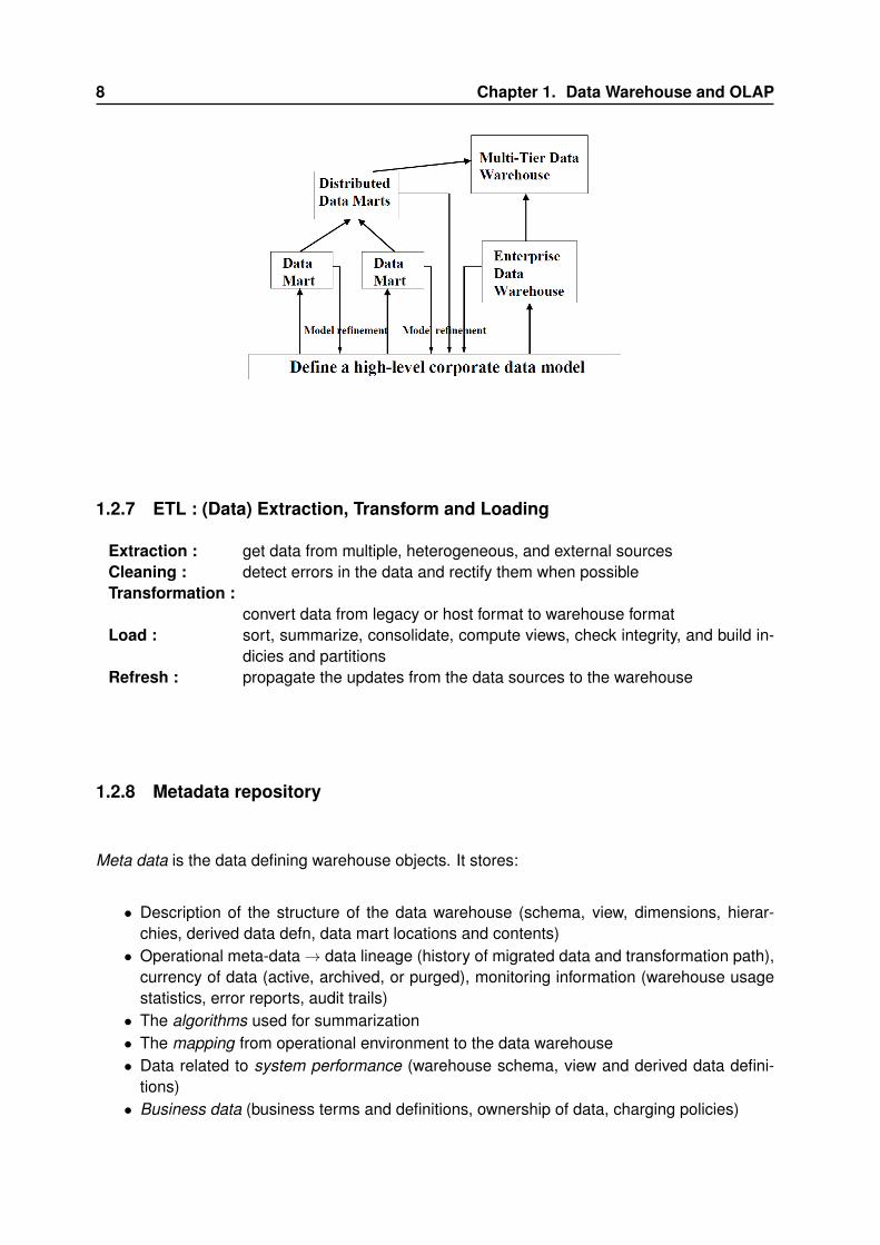
1.2.7 ETL : (Data) Extraction, Transform and Loading
Extraction : get data from multiple, heterogeneous, and external sourcesCleaning : detect errors in the data and rectify them when possibleTransformation :
convert data from legacy or host format to warehouse formatLoad : sort, summarize, consolidate, compute views, check integrity, and build in-
dicies and partitionsRefresh : propagate the updates from the data sources to the warehouse
1.2.8 Metadata repository
Meta data is the data defining warehouse objects. It stores:
• Description of the structure of the data warehouse (schema, view, dimensions, hierar-chies, derived data defn, data mart locations and contents)• Operational meta-data→ data lineage (history of migrated data and transformation path),
currency of data (active, archived, or purged), monitoring information (warehouse usagestatistics, error reports, audit trails)• The algorithms used for summarization• The mapping from operational environment to the data warehouse• Data related to system performance (warehouse schema, view and derived data defini-
tions)• Business data (business terms and definitions, ownership of data, charging policies)

1.3. DW modeling : Data Cube and OLAP 9
1.3 DW modeling : Data Cube and OLAP
1.3.1 From table and spreadseets to datacube
A data warehouse is based on a multidimensional data model which views data in the form of adata cube.
A data cube, such as sales, allows data to be modeled and viewed in multiple dimensions :
• Dimension tables, such as item (item_name, brand, type), or time (day, week, month,quarter, year)• The fact table contains measures (such as dollars_sold) and keys to each of the related
dimension tables
1.3.2 Examples
1.3.2.1 A 2-D cube representation (time, item)
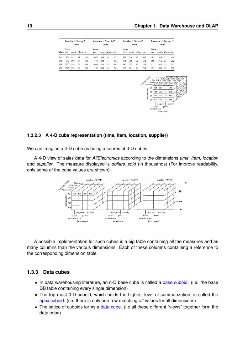
A 2-D view of sales data for AllElectronics according to the dimensions time and item, where thesales are from branches located in the city of Vancouver. The measure displayed is dollars_sold(in thousands) :
1.3.2.2 A 3-D cube representation (time, item, location)
A 3-D view of sales data for AllElectronics according to the dimensions time, item and location.The measure displayed is dollars_sold (in thousands) :
10 Chapter 1. Data Warehouse and OLAP
1.3.2.3 A 4-D cube representation (time, item, location, supplier)
We can imagine a 4-D cube as being a serires of 3-D cubes.
A 4-D view of sales data for AllElectronics according to the dimensions time, item, locationand supplier. The measure displayed is dollars_sold (in thousands) (For improve readability,only some of the cube values are shown):
A possible implementation for such cubes is a big table containing all the measures and asmany columns than the various dimensions. Each of these columns containing a reference tothe corresponding dimension table.
1.3.3 Data cubes
• In data warehousing literature, an n-D base cube is called a base cuboid. (i.e. the baseDB table containing every single dimension)• The top most 0-D cuboid, which holds the highest-level of summarization, is called the
apex cuboid. (i.e. there is only one row matching all values for all dimensions)• The lattice of cuboids forms a data cube. (i.e all these different "views" together form the
data cube)

1.3. DW modeling : Data Cube and OLAP 11
The Data Cube is a lattice of cuboids :
The whole idea is to really have all this indexing and values redundance stored in thedatabase in order to be able to serve data queries very fast and efficiently.
1.3.4 Conceptual modeling of Data warehouses
Modeling data warehouses: dimensions & measures :
Star schema: A fact table in the middle connected to a set of dimension tablesSnowflake schema:
A refinement of star schema where some dimensional hierarchy is nor-malized into a set of smaller dimension tables, forming a shape similar tosnowflake
Fact constellations:Multiple fact tables share dimension tables, viewed as a collection of stars,therefore called galaxy schema or fact constellation
1.3.4.1 Star schema
The most common modeling paradigm is the star schema, the data warehouse contains :
• a large central table (fact table) containing the bulk of the data, with no redundancy• a set of smaller attendant tables (dimension tables), one for each dimension
The schema graph resembles a starburst, with the dimension tables displayed in a radialpattern around the central fact table. Example :

12 Chapter 1. Data Warehouse and OLAP
1.3.4.2 Snowflake schema
• A variant of the star schema model, where some dimension tables are normalized, therebyfurther splitting the data into additional tables• The resulting schema graph forms a shape similar to a snowflake.• The dimension tables of the snowflake model may be kept in normalized form to reduce
redundancies.• But, the snowflake structure can reduce the effectiveness of browsing, since more joins
will be needed to execute a query.• Although the snowflake schema reduces redundancy, it is not as popular as the star
schema in data warehouse design. (performance concerns)
Example :
1.3.4.3 Fact constellation schema
Sophisticated applications may require multiple fact tables to share dimension tables.This kind of schema can be viewed as a collection of stars, and hence is called a galaxy schemaor a fact constellation.
Example :

1.3. DW modeling : Data Cube and OLAP 13
1.3.4.4 Use of the schemas
• A data warehouse collects information about subjects that span the entire organization,such as customers, items, sales, assets, and personnel, and thus its scope is enterprise-wide.→ For data warehouses, the fact constellation schema is commonly used, since it canmodel multiple, interrelated subjects.• A data mart, on the other hand, is a department subset of the data warehouse that focuses
on selected subjects, and thus its scope is department-wide.→ For data marts, the star or snowflake schema are commonly used, since both aregeared toward modeling single subjects, although the star schema is more popular andefficient.
1.3.5 A concept hierarchy
A concept hierarchy defines a sequence of mappings from a set of low-level concepts to higher-level, more general concepts.
Exemple: location :
• City values for location : Vancouver, Toronto, NewYork, and Chicago• Each city, can be mapped to the province or state to which it belongs: Vancouver can be
mapped to British Columbia, and Chicago to Illinois• The provinces and states can in turn be mapped to the country to which they belong, such
as Canada or the USA
These mappings form a concept hierarchy for the dimension location, mapping a set of low-level concepts (i.e., cities) to higher-level,more general concepts (i.e., countries).

14 Chapter 1. Data Warehouse and OLAP
1.3.6 Data Cube measures
A data cube measure is a numerical function that can be evaluated at each point in the datacube space.→ E.g., a multidimensional point in the data cube space :time = "Q1", location = "Vancouver",item = "computer"
A measure value is computed for a given point by aggregating the data corresponding to therespective dimension-value pairs defining the given point.
1.3.6.1 Three categories
Distributive: if the result can be derived by applying the function to n aggregate values,i.e. it is the same as that derived by applying the function on all the datawithout partitioning→ Distributive measures can be computed efficiently because of the waythe computation can be partitionedE.g., count(), sum(), min(), max()
Algebraic: if it can be computed by an algebraic function with M arguments (where Mis a bounded integer), each of which is obtained by applying a distributiveaggregate function.E.g., avg(), min_N(), standard_deviation()See practice
Holistic: if there is no constant bound on the storage size needed to describe a sub-aggregate. → It is difficult to compute holistic measures efficiently. Efficienttechniques to approximate. The computation of some holistic measures,however, do exist.E.g., median(), mode(), rank()

1.3. DW modeling : Data Cube and OLAP 15
1.3.7 DMQL : Data Mining Query Language
DMQL is a language for creating cubes. There are other specific languages supported by someRDBMS or environment, but here we will focus in DMQL :
Cube Definition (Fact Table) :define cube <cube_name> [<dimension_list>]: <measure_list>
Dimension Definition (Dimension Table) :define dimension <dimension_name> as (<attribute_or_subdimension_list>)
Special Case (Shared Dimension Tables) :(First time as "cube definition" above)define dimension <dimension_name> as <dimension_name_first<_time> in cube
<cube_name_first_time>
1.3.7.1 Example of a star schema definition in DMQL
define cube sales star [time, item, branch, location]:
dollars sold = sum(sales in dollars), units sold = count(*)
define dimension time as (time key, day, day of week, month, quarter, year)
define dimension item as
(item key, item name, brand, type, supplier type)
define dimension branch as
(branch key, branch name, branch type)
define dimension location as
(location key, street, city, province or state, country)
1.3.7.2 Example of a snowflake schema definition in DMQL
define cube sales snowflake [time, item, branch, location]:
dollars sold = sum(sales in dollars), units sold = count(*)
define dimension time as
(time key, day, day of week, month, quarter, year)
define dimension item as
(item key, item name, brand, type, supplier (supplier key, supplier type))
define dimension branch as
(branch key, branch name, branch type)
define dimension location as
(location key, street, city (city key, city, province or state, country))
• The item and location dimension tables are normalized• Defining supplier in this way implicitly creates a supplier key in the item dimension table
definition• A city key is implicitly created as well.

16 Chapter 1. Data Warehouse and OLAP
1.3.7.3 Example of a fact constellation schema definition in DMQL
define cube sales [time, item, branch, location]:
dollars sold = sum(sales in dollars), units sold = count(*)
define dimension time as
(time key, day, day of week, month, quarter, year)
define dimension item as
(item key, item name, brand, type, supplier type)
define dimension branch as
(branch key, branch name, branch type)
define dimension location as
(location key, street, city, province or state, country)
define cube shipping [time, item, shipper, from location, to location]:
dollars cost = sum(cost in dollars), units shipped = count(*)
define dimension time as time in cube sales
define dimension item as item in cube sales
define dimension shipper as
(shipper key, shipper name, location as location in cube sales, shipper type)
define dimension from location as location in cube sales
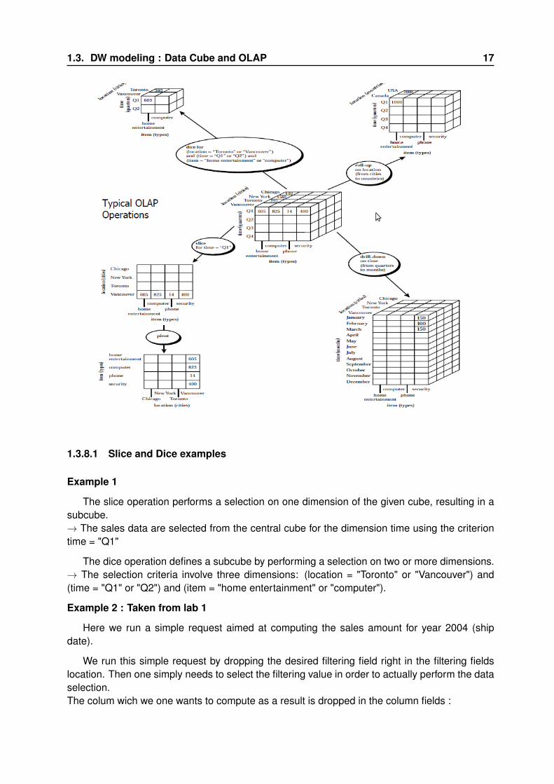
1.3.8 Typical OLAP Operations
Roll up: (drill-up) summarize data by climbing up hierarchy or by dimension reduc-tion
Drill down: (roll down) reverse of roll-up, from higher level summary to lower level sum-mary or detailed data, or introducing new dimensions
Slice and dice: project and selectPivot: (rotate) reorient the cube, visualization, 3D to series of 2D planes
Other operations :
drill across: involving (across) more than one fact tabledrill through: through the bottom level of the cube to its backend relational tables (using
SQL)
1.3. DW modeling : Data Cube and OLAP 17
1.3.8.1 Slice and Dice examples
Example 1
The slice operation performs a selection on one dimension of the given cube, resulting in asubcube.→ The sales data are selected from the central cube for the dimension time using the criteriontime = "Q1"
The dice operation defines a subcube by performing a selection on two or more dimensions.→ The selection criteria involve three dimensions: (location = "Toronto" or "Vancouver") and(time = "Q1" or "Q2") and (item = "home entertainment" or "computer").
Example 2 : Taken from lab 1
Here we run a simple request aimed at computing the sales amount for year 2004 (shipdate).
We run this simple request by dropping the desired filtering field right in the filtering fieldslocation. Then one simply needs to select the filtering value in order to actually perform the dataselection.The colum wich we one wants to compute as a result is dropped in the column fields :

18 Chapter 1. Data Warehouse and OLAP
And the result is 10’158’562.38 USD.
Then we should compute the total sales amount for a specific article - "Fender Set-Mountain"- for year 2004 (order date) but only in the California (state province name).
This is actually quite simply performed as one only needs to add the additional filtering fieldsand values in the same filtering fields location.
And the result is 7’385.28 USD.

1.3. DW modeling : Data Cube and OLAP 19
1.3.8.2 Roll-Up examples
Example 1
A roll-up operation performed on the central cube by climbing up the concept hierarchy forlocation from the level of city to the level of country.
Hierarchy definition (total order) : "street < city < province or state < country."
The roll-up operation aggregates the data by ascending the location hierarchy, the resultingcube groups the data by country.
Example 2
A roll-up performed by dimension reduction, is considered on a sales data cube (with twodimensions location and time) by removing, the time dimension, resulting in an aggregation ofthe total sales by location, rather than by location and by time.
Example 3 : Taken from lab 1
Now we should emphasize the roll-up principle by getting rid of the filtering on the state value(California).
Based on this principle we should answer the very same question related to the amount ofsales for article "Fender Set-Mountain" for year 2004 but this time for every known states alltogether.
Again this is quite simply executed as one only needs to get rid of the related filtering fieldfrom the filtering fields location :
And the result is 27’211.24 USD.
20 Chapter 1. Data Warehouse and OLAP
1.3.8.3 Drill-Down examples
Example 1
A drill-down operation performed on the central cube by stepping down a concept hierarchyfor time defined as "day < month < quarter < year." , by descending the time hierarchy from thelevel of quarter to the more detailed level of month.
The resulting data cube details the total sales per month rather than summarizing them byquarter.
Example 2
A drill-down performed by adding new dimensions to a cube is done on the central cube byintroducing an additional dimension, such as customer group.
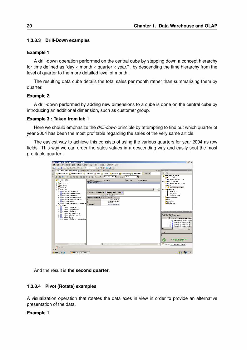
Example 3 : Taken from lab 1
Here we should emphasize the drill-down principle by attempting to find out which quarter ofyear 2004 has been the most profitable regarding the sales of the very same article.
The easiest way to achieve this consists of using the various quarters for year 2004 as rowfields. This way we can order the sales values in a descending way and easily spot the mostprofitable quarter :
And the result is the second quarter.
1.3.8.4 Pivot (Rotate) examples
A visualization operation that rotates the data axes in view in order to provide an alternativepresentation of the data.
Example 1

1.3. DW modeling : Data Cube and OLAP 21
• A pivot operation where the item and location axes in a 2-D slice are rotated.• Rotating the axes in a 3-D cube, or transforming a 3-D cube into a series of 2-D planes.
Example 2 : Taken from lab 1
Finally we will illustrate how a pivot operation is typically achieved by switching the fieldsfrom both axis.
Happily this is easily done with Microsoft Visual Studio as a specific menu item is providedin this intent :
As a matter of fact we get the same result.
1.3.9 Starnet Query Model
The querying of multidimensional databases can be based on a starnet model. A starnet modelconsists of radial lines emanating from a central point, where each line represents a concepthierarchy for a dimension.
Each abstraction level in the hierarchy is called a footprint. These represent the granularitiesavailable for use by OLAP operations such as drill-down and rollup.

22 Chapter 1. Data Warehouse and OLAP
1.4 Design and Usage
A Data Warehouse (DW) is a business analysis framework. Why should one bother implement-ing a DW ?
• Provide competitive advantage→ measure performance and make critical adjustments• Enhance business productivity→ information that accurately describes the organization• Facilitate customer relationship management→ consistent view of customers and items across all lines of business, all departments,and all market• Bring about cost reduction→ by tracking trends, patterns, and exceptions over
1.4.1 Four views
The design of a data warehouse can be seen from four distinct views :
• Top-down view→ allows selection of the relevant information necessary for the data warehouse (currentand future business needs)• Data source view→ exposes the information being captured, stored, and managed by operational systems• Data warehouse view→ consists of fact tables and dimension tables• Business query view→ sees the perspectives

1.4. Design and Usage 23
1.4.2 Skills to build and use a DW
Business Skills
• To know systems storage and management data• To build extractors, warehouse, to refresh software• To understand the significance of the data• To translate the business requirements into queries
Technology skills
• To understand how to make assessments from quantitative information• To discover patterns and trends, to extrapolate them based on history and look for anoma-
lies• To present coherent managerial recommendations
Program management skills
• To interface with technologies, vendors, and end users, to deliver results in a timely andcost-effective manner
1.4.3 Data Warehouse Design Process
1.4.3.1 What approach ?
What approach is to be used ? Top-down, bottom-up approaches or a combination of both ?
Top-down: Starts with overall design and planning, useful when the technology is ma-ture and well known, and where the business problems that must be solvedare clear and well understood.
Bottom-up: Starts with experiments and prototypes (rapid), useful in the early stage ofbusiness modeling and technology development. It is less expensive andevaluate the benefits of the technology before making significant commit-ments.
1.4.3.2 From software engineering point of view
The steps are : planning, requirements study, problem analysis, warehouse design, data inte-gration and testing, and the deployment of the DW
Waterfall: structured and systematic analysis at each step before proceeding to thenext
Spiral: rapid generation of increasingly functional systems, short turn around time,quick turn around→ a good choice for DW development, especially for data marts, becausethe turnaround

24 Chapter 1. Data Warehouse and OLAP
1.4.3.3 Typical data warehouse design process
1. Choose a business process to modele.g., orders, invoices
2. Choose the grain (atomic level of data) of the business processe.g., individual transactions, individual daily snapshots
3. Choose the dimensions that will apply to each fact table record,e.g., time, item, customer, supplier, warehouse, transaction, type, and status.
4. Choose the measure that will populate each fact table recorde.g, dollars sold and units sold.
1.4.4 Data Warehouse Deployment
• Initial installation, planning, training• DW administration: data refreshment, data source synchronization, planning for disas-
ter recovery, managing access control and security, managing data growth, managingdatabase performance, and DW enhancement and extension• Scope management: controlling the number and range of queries, dimensions, and re-
ports; limiting the size of the DW• DW development tools: functions to define and edit metadata repository contents (such
as schemas, scripts, or rules), answer queries, output reports, and ship metadata to andfrom relational database system catalogue
1.4.5 Data Warehouse Usage
Three kinds of data warehouse applications :
Information processing :
• supports querying, basic statistical analysis, and reporting using crosstabs, tables, chartsand graphs
Analytical processing :
• multidimensional analysis of data warehouse data• supports basic OLAP operations, slice-dice, drilling, pivoting
Data mining :
• knowledge discovery from hidden patterns• supports associations, constructing analytical models, performing classification and pre-
diction, and presenting the mining results using visualization tools

1.5. Practice 25
1.4.6 OLAM : Online Analytical Mining
From On-Line Analytical Processing (OLAP) to On Line Analytical Mining (OLAM) - Why onlineanalytical mining?
• High quality of data in data warehouses.→ DW contains integrated, consistent, cleaned data• Available information processing structure surrounding data warehouses→ ODBC, OLEDB, Web accessing, service facilities, reporting and OLAP tools• OLAP-based exploratory data analysis→ Mining with drilling, dicing, pivoting, etc.• On-line selection of data mining functions→Integration and swapping of multiple mining functions, algorithms, and tasks
1.5 Practice
1.5.1 OLAP operations
Suppose that a data warehouse consists of the four dimensions, date, spectator, location, andgame, and the two measures, count and charge, where charge is the fare that a spectator payswhen watching a game on a given date. Spectators may be students, adults, or seniors, witheach category having its own charge rate.
1.5.1.1 Star schema
Draw a star schema diagram for the data warehouse :

26 Chapter 1. Data Warehouse and OLAP
1.5.1.2 OLAP operations
Starting with the base cuboid [date; spectator; location; game], what specific OLAP operationsshould one perform in order to list the total charge paid by student spectators at GM_Place in2004?
• Roll-up on date from date id to year.• Roll-up on game from game id to all.• Roll-up on location from location id to location name.• Roll-up on spectator from spectator id to status.• Dice with status="students", location name="GM Place", and year="2004"
1.5.2 Data Warhouse And Data Mart
What are the difference and similarities between a Data Mart and a Data warehouse ?
Similarities :
• Both are a storage of data i n a subject-oriented, integrated, time-variant and non-volatileway.
Differences :
• A Data Mart is oriented on a single business-domain or a single subject (for instance mar-keting) while a Data Warehouse is global to the enterprise and covers the whole enterprisedomain.• A Data Mart is expected to be much simplier than a Data Warehouse and sometimes even
summarized while a Data Warehouse contains detailed and summarized data.• A Data Mart is usually cheaper to implement.• A Data warehouse can be implemented bottom-up by aggregating Data Marts while a
Data Mart is usually designed top-down.
1.5.3 OLAP operations, another example
Suppose a data warehouse consosts of the three dimensions time, doctor and patient and twomeasures of count and charge, where charged is the fee that a doctor charges a patient for avisit.Starting with the base cuboid [day, doctor, patient[, what specific OLAP operations should beperformed in order to list the total fee collected by each doctor in 2010 ?
• roll up on time from day to year• roll up on patient from patient_id to all• slice with year = "2010"

1.5. Practice 27
1.5.4 Data Warhouse modeling
A data warehouse can be modelled by either a star schema or a snowflake schema. Brieflydescribe the similarities and the differences of the two models, and then analyze their advan-tages and disadvantages with regard to one another. Give your opinion of which might be moreempirically useful and state the reasons behind your answer.
They are similar in the sense that they all have a fact table, as well as some dimensionaltables. The major difference is that some dimension tables in the snowflake schema are normal-ized, thereby further splitting the data into additional tables. The advantage of the star schema isits simplicity, which will enable efficiency, but it requires more space. For the snowflake schema,it reduces some redundancy by sharing common tables: the tables are easy to maintain andsave some space. However, it is less efficient and the saving of space is negligible in com-parison with the typical magnitude of the fact table. Therefore, empirically, the star schema isbetter simply because efficiency typically has higher priority over space as long as the spacerequirement is not too huge. In industry, sometimes the data from a snowflake schema may bedenormalized into a star schema to speed up processing.
1.5.5 Computation of measures
1.5.5.1 Categories of measures
Enumerate three categories of measures, based on the kind of aggregate functions used incomputing a data cube.
The three categories of measures are distributive, algebraic, and holistic.
1.5.5.2 variance
For a data cube with the three dimensions time, location, and item, which category does thefunction variance belong to? Describe how to compute it if the cube is partitioned into manychunks.
The variance belongs to the algebraic category.
Recall :
The sample mean x of observations x1,x2,...,xn is given by
x =x1 + x2 + ...+ xn
n=
1
n
n∑i=1
xi
The numerator of x can be written more informally as∑xi, where the summation is over all
sample observations.
The variance can be obtained as
σX =1
n
n∑i=1
(xi − x)2

28 Chapter 1. Data Warehouse and OLAP
One can write
σX =1
n
n∑i=1
(xi − x)2
=1
n
n∑i=1
(x2i − 2xix+ x2)
=1
n
n∑i=1
x2i −2
nx
n∑i=1
xi +1
n
n∑i=1
x2
=1
n
n∑i=1
x2i −2
nxnx+
1
nnx2
=1
n
n∑i=1
x2i − 2x2 + x2
=1
n
n∑i=1
x2i − x2(⇒ alternate variance formula)
So now we end up with various different k little cubes :
1 - we compute the partial values for each little cube345...k
The values are computed this way :
σX =1
n
n∑i=1
x2i − (
∑ni=1 xin
)2
where
• 1n is easily computed : n is the total amount of rows in all cubes
•∑n
i=1 x2i is easy : one only need to sum the partial sums.
• (∑n
i=1 xin )2 is easy as well : simply keep track of the partial
∑ni=1 xi and compute n =
(n1 + n2 + ...+ nk)
This way we don’t need to recompute everything each time a new chunk of data is added.One only needs to compute the partial results for the new chunk and then integrate these resultsin the totals.
The very same principle can be applied to the function computing the 10 top values (the 10top values are mandatorily in the 10 top values for each chunk) and other functions as well.

1.5. Practice 29
This is called Distributive aggregate functions


CHAPTER 2
Data Preprocessing
Contents2.1 Overview . . . . . . . . . . . . . . . . . . . . . . . . . . . . . . . . . . . . . . . . . . 29
2.1.1 Why preprocess the data ? . . . . . . . . . . . . . . . . . . . . . . . . . . . . 29
2.1.2 Major Tasks in Data Preprocessing . . . . . . . . . . . . . . . . . . . . . . . . 30
2.2 Data Cleaning . . . . . . . . . . . . . . . . . . . . . . . . . . . . . . . . . . . . . . . 31
2.2.1 Incomplete (Missing) Data . . . . . . . . . . . . . . . . . . . . . . . . . . . . . 32
2.2.2 How to Handle Missing Data? . . . . . . . . . . . . . . . . . . . . . . . . . . . 32
2.2.3 Noisy Data . . . . . . . . . . . . . . . . . . . . . . . . . . . . . . . . . . . . . 33
2.2.4 How to Handle Noisy Data? . . . . . . . . . . . . . . . . . . . . . . . . . . . . 33
2.2.5 Data cleaning as a process . . . . . . . . . . . . . . . . . . . . . . . . . . . . 34
2.3 Data Integration . . . . . . . . . . . . . . . . . . . . . . . . . . . . . . . . . . . . . . 35
2.3.1 Handling Redundancy in Data Integration . . . . . . . . . . . . . . . . . . . . 36
2.3.2 Correlation Analysis (Nominal Data) . . . . . . . . . . . . . . . . . . . . . . . 36
2.3.3 Correlation Analysis (Numerical Data) . . . . . . . . . . . . . . . . . . . . . . 37
2.3.4 Covariance (Numeric Data) . . . . . . . . . . . . . . . . . . . . . . . . . . . . 39
2.4 Data Reduction . . . . . . . . . . . . . . . . . . . . . . . . . . . . . . . . . . . . . . 40
2.4.1 Data Reduction Strategies . . . . . . . . . . . . . . . . . . . . . . . . . . . . . 40
2.4.2 Dimensionality Reduction . . . . . . . . . . . . . . . . . . . . . . . . . . . . . 40
2.4.3 Numerosity Reduction . . . . . . . . . . . . . . . . . . . . . . . . . . . . . . . 42
2.4.4 Data Compression . . . . . . . . . . . . . . . . . . . . . . . . . . . . . . . . . 46
2.5 Data Transformation and data Discretization . . . . . . . . . . . . . . . . . . . . . 47
2.5.1 Data Transformation . . . . . . . . . . . . . . . . . . . . . . . . . . . . . . . . 47
2.5.2 Data Discretization . . . . . . . . . . . . . . . . . . . . . . . . . . . . . . . . . 48
2.5.3 Concept Hierarchy Generation . . . . . . . . . . . . . . . . . . . . . . . . . . 50
2.6 Practice . . . . . . . . . . . . . . . . . . . . . . . . . . . . . . . . . . . . . . . . . . . 51
2.6.1 Computation on Data . . . . . . . . . . . . . . . . . . . . . . . . . . . . . . . 51
2.6.2 Smoothing . . . . . . . . . . . . . . . . . . . . . . . . . . . . . . . . . . . . . 53
2.6.3 Data Reduction and tranformation . . . . . . . . . . . . . . . . . . . . . . . . 54
2.6.4 Sampling . . . . . . . . . . . . . . . . . . . . . . . . . . . . . . . . . . . . . . 56

32 Chapter 2. Data Preprocessing
2.1 Overview
2.1.1 Why preprocess the data ?
Data usually has to respect these principles : Accuracy, Completeness, Consistency, Timeli-ness, Believability, Interpretability.
2.1.1.1 Accuracy, completeness, consistency
Introducing Example
• You are a manager at AllElectronics and have been charged with analyzing the company’sdata with respect to the sales at your branch.• You identify and select the attributes to be included in your analysis (item, price, and units
sold).• You notice that several of the attributes for various tuples have no recorded value.• For your analysis, you would like to include information as to whether each item purchased
was advertised as on sale, yet you discover that this information has not been recorded.• Users of your database system have reported errors, unusual values, and inconsistencies
in the data recorded for some transactions.
→ This underscores the kind of issues one can have with the data.
Preprocessing helps avoiding situations where the data one wish to analyze by data miningtechniques are:
incomplete: lacking attribute values or certain attributes of interest, or containing onlyaggregate data
inaccurate: (or noisy) containing errors, or outlier values that deviate from the expectedinconsistent: e.g., containing discrepancies in the department codes used to categorize
items
2.1.1.2 Timeliness
Introducing Example
• Suppose that you are overseeing the distribution of monthly sales bonuses to the top salesrepresentatives at AllElectronics.• Several sales representatives, however, fail to submit their sales records on time at the
end of the month.There are also a number of corrections and adjustments that flow in after the month’s end.• For a period of time following each month, the data stored in the database is incomplete.• However, once all of the data is received, it is correct.• The fact that the month-end data is not updated in a timely fashion has a negative impact
on the data quality.

2.1. Overview 33
→ Timeliness issues can be managed by having a preprocessing step which postpones theupdate of the data in the warehouse until the input data set is complete
2.1.1.3 Believability
Introducing Example
• A few years back, a programming error miscalculated the sales commissions for its salesrepresentatives so that these employees received 20% less than was due.• The software bug was quickly fixed and the data corrected.• Even though the database is now accurate, complete, consistent, and timely, it is still not
trusted because of the memory users have of the past error.• Sales managers prefer to compute the expected commissions by hand based on their
employees handsubmitted reports rather than believe the data stored in the database.
→ People losing faith in the data is a severe issue. Data need to be believable / reliable.
2.1.1.4 Interpretability
Introducing Example
• Consider a sales database, where it is common to create "adjustment" orders to handlecomplaints and returns.• This procedure assigns new order numbers to the adjustment and replacement orders.• The accounting department knows how to interpret the resulting data.• A business analyst may have a hard time understanding the data, thinking that each order
number represents a distinct order.• Thus, to the business analyst, the data is of low quality due to poor interpretability.
2.1.2 Major Tasks in Data Preprocessing
Data cleaning: - see 2.2
• Fill in missing values. - see 2.2.2• Smooth noisy data, identify or remove outliers, and resolve inconsistencies - see 2.2.4
Data integration: - see 2.3
• Integration of multiple databases, data cubes, or files
Data reduction: (a reduced representation of data set, smaller in volume, producing the same(almost) analytical results)
• Dimensionality reduction (by applying data encoding schemes)• Numerosity reduction (replace data by alternative, smaller representations using paramet-
ric or non parametric models

34 Chapter 2. Data Preprocessing
• Data compression
Data transformation and data discretization
• Normalization (scale data to ranges)• Concept hierarchy generation
TODO list all techniques here with references
2.2 Data Cleaning
Data in the real world is dirty:
incomplete: lacking attribute values, lacking certain attributes of interest, or containingonly aggregate data→ e.g., Occupation=" " (missing data)
noisy: containing noise, errors, or outliers→ e.g., Salary="-10" (an error)
inconsistent: containing discrepancies in codes or names, e.g.,→ e.g. Age="42" Birthday="03/07/1997" → e.g. was rating "1,2,3", nowrating "A, B, C"→ e.g. discrepancy between duplicate records

2.2. Data Cleaning 35
2.2.1 Incomplete (Missing) Data
Data is not always available.
• E.g., many tuples have no recorded value for several attributes, such as customer incomein sales data
Missing data may be due to
• equipment malfunction• inconsistent with other recorded data and thus deleted• data not entered due to misunderstanding• certain data may not be considered important at the time of entry• not register history or changes of the data
Missing data may need to be inferred.
2.2.2 How to Handle Missing Data?
• Ignore the tuple: usually done when class label is missing (when doing classification);not effective when the % of missing values per attribute varies considerably→ This method is not very effective unless the tuple contains several attributes withmissing values. It is especially poor when the percentage of missing values per attributevaries considerably.
• Fill in the missing value manually: tedious + infeasible?→ In general, this approach is time-consuming and may not be a reasonable task forlarge data sets with many missing values, especially when the value to be filled in is noteasily determined.
• Fill in it automatically with
• a global constant : e.g., "unknown", a new class?!→ If missing values are replaced by, say, "Unknown", then the mining program maymistakenly think that they form an interesting concept, since they all have a valuein common, that of "Unknown." Hence, although this method is simple, it is notrecommended.• the attribute mean : (Using the attribute mean for quantitative (numeric) values or
attribute mode for categorical (nominal) values.)• the attribute mean for all samples belonging to the same class : smarter
(Using the attribute mean for quantitative (numeric) values or attribute mode forcategorical (nominal) values, for all samples belonging to the same class as thegiven tuple.) → For example, if classifying customers according to credit risk,replace the missing value with the average income value for customers in the samecredit risk category as that of the given tuple.

36 Chapter 2. Data Preprocessing
• the most probable value : inference-based such as Bayesian formula or decisiontree (Using the most probable value to fill in the missing value: This may be deter-mined with regression, inference-based tools using Bayesian formalism, or decisiontree induction.)→ For example, using the other customer attributes in the data set, we can constructa decision tree to predict the missing values for income.
2.2.3 Noisy Data
• Noise: random error or variance in a measured variable• Incorrect attribute values may be due to
• faulty data collection instruments• data entry problems• data transmission problems• technology limitation• inconsistency in naming convention
• Other data problems which require data cleaning
• duplicate records• incomplete data• inconsistent data
2.2.4 How to Handle Noisy Data?
Binning: (lissage)
• first sort data and partition into (equal-frequency) bins• then one can smooth by bin means, smooth by bin median, smooth by bin boundaries,
etc.
Regression:
• smooth by fitting the data into regression functions
Clustering:
• detect and remove outliers
Combined computer and human inspection:
• detect suspicious values and check by human (e.g., deal with possible outliers)
2.2.4.1 Regression
• Linear regression involves finding the "best" line to fit two attributes (or variables), so thatone attribute can be used to predict the other.

2.2. Data Cleaning 37
• Multiple linear regression is an extension of linear regression, where more than twoattributes are involved and the data are fit to a multidimensional surface.
The principle : Let’s imagine a line in the cloud of points on a plan. We look for the lineminimizing the sum of the distance between every point and the line. Then we get rid of thepoints that have a distance to the line above the average (mean) distance (or we fix them).
2.2.4.2 Clustering
The principle : First, the points on the plan are grouped together according to some distancecalculation. Then the points which could not be grouped to any other are discarded (or fixed).
2.2.5 Data cleaning as a process
We’ll now focus on the usual process for data cleaning.
2.2.5.1 Data discrepancy detection
What are the ways for detecting data discrepency ?
• Use metadata: the data type and domain of each attribute, the acceptable values for eachattribute• Basic statistical data descriptions to grasp data trends and identify anomalies (values that
are more than two standard deviations away from the mean for a given attribute may beflagged as potential outliers)• Write your own scripts
What are typically the kind of descrepencies detected ?

38 Chapter 2. Data Preprocessing
• Inconsistent use of codes→ e.g., "2010/12/25" and "25/12/2010" for date• Field overloading, when developers squeeze few attribute definitions into unused (bit) por-
tions of already defined attributes→ e.g., using an unused bit of an attribute whose value range uses only, say, 31 out of 32bits
Data should be examined regarding :
• unique rules: each value of the given attribute must be different from all other values forthat attribute• consecutive rules: there can be no missing values between the lowest and highest
values for the attribute and that all values must also be unique(e.g., as in check numbers)• null rules: specify the use of blanks, question marks, special characters, or other strings
that may indicate the null condition (e.g., where a value for a given attribute is not avail-able), and how such values should be handled
A possibility: use commercial tools to detect discrepencies :
• Data scrubbing: use simple domain knowledge (e.g., postal code, spellcheck) to detecterrors and make corrections• Data auditing: by analyzing data to discover rules and relationship to detect violators
(e.g., correlation and clustering to find outliers)
A possibility: use commercial tools for data transformation step :
• Data migration tools: allow simple transformations to be specified (e.g., replace the string“gender" by "sex")• ETL (Extraction/Transformation/Loading) tools: allow users to specify transformations
through a graphical user interface• They support only a restricted set of transforms: write custom scripts
2.3 Data Integration
Goal : Combines data from multiple sources into a coherent store
Schema integration :
• Integrate metadata from different sources• e.g., A.cust-id ≡ B.cust-#
Entity identification problem:
• Identify real world entities from multiple data sources• e.g., Bill Clinton = William Clinton
Detecting and resolving data value conflicts:

2.3. Data Integration 39
• For the same real world entity, attribute values from different sources are different• Possible reasons: different representations,
2.3.1 Handling Redundancy in Data Integration
• Redundant data occur often when integration of multiple databases
• Object identification: The same attribute or object may have different names in dif-ferent databases• Derivable data: One attribute may be a "derived" attribute in another table, e.g.,
annual revenue
• Redundant attributes may be able to be detected by correlation analysis and covarianceanalysis• Careful integration of the data from multiple sources may help reduce/avoid redundancies
and inconsistencies and improve mining speed and quality
2.3.2 Correlation Analysis (Nominal Data)
We use the χ2 (chi-square) test
χ2 =∑ (Observerd− Expected)2
Expected
• The larger the χ2 value, the more likely the variables are related• The cells that contribute the most to the χ2 value are those whose actual count is very
different from the expected count• Correlation does not imply causality
• # of hospitals and # of car-theft in a city are correlated• Both are causally linked to the third variable: population
2.3.2.1 χ2 test : an example
Play Chess Not Play Chess Sum (row)Like Sci-Fi 250(90) 200(360) 450Not Like Sci-Fi 50(210) 1000(840) 1050Sum(col) 300 1200 1500
• The values in parenthesis are expected values. To compute them one should just do asif the individual results were missing and compute the expected values out of the partialsums. For instance : Cell "Play Chess & Likes Sci-Fi2 is (Sum for Play Chess * Sum forLikes Sci-Fi / Global Sum)• The χ2 (chi-square) calculation (numbers in parenthesis are expected counts calculated
based on the data distribution in the two categories)

40 Chapter 2. Data Preprocessing
χ2 =(250− 90)2
90+
(50− 210)2
210+
(200− 360)2
360+
(1000− 840)2
840= 507.93
• The χ2 statistic tests the hyp that A and B are independent. The test is based on a signifi-cance level , with (r-1)x(c-1)= (2-1)x(2-1)=1 degrees of freedom. For 1 degree of freedom,the χ2 value needed to reject the hypothesis at 0.001 significance level is 10.828. Since507.93>10.828, we can reject the hypothesis that like_science_fiction and play_chess areindependent and conclude that they are strongly correlated for the given group of people.
Note : The values in parenthesis are computed this way :
90 = (300 ∗ 450)/1500
210 = (300 ∗ 1050)/1500
etc.
2.3.3 Correlation Analysis (Numerical Data)
In this case we use the Correlation coefficient also called the Pearson’s product moment co-efficient :
Let’s assume p and q are the values taken for two distinct attributes by a population.
rp,q =
∑(p− p)(q − q)(n− 1)σpσq
=
∑(pq)− npq
(n− 1)σpσq
where
• n is the number of tuples,• p and q are the respective means of p and q,• σp and σq are the respective standard deviation of p and q,•∑pq is the sum of the pq cross-product.
Principle :
• rp,q > 0→ p and q are positively correlated (p’s values increase as q’s).• rp,q = 0→ independent;• rp,q < 0→ negatively correlated
Note : 1 ≤ 1rp,q ≤ 1
2.3.3.1 Visually Evaluating Correlation
This figures displays a scatter plots showing similarities from -1 to +1 :

2.3. Data Integration 41
2.3.3.2 Correlation viewed as a linear relationship
Correlation measures the linear relationship between objects. So to compute correlation, wecan standardize data objects, p and q, and then take their dot product :
p′k = (pk −mean(p))/std(p)
q′k = (qk −mean(q))/std(q)
correlation(p, q) = p′ · q′
2.3.4 Covariance (Numeric Data)
Covariance is similar to correlation :
Cov(p, q) = E((p− p)(q − q)) =
∑ni=1(pi − p)(qi − q)
n
rp,q =Cov(p, q)
σpσq
where

42 Chapter 2. Data Preprocessing
• n is the number of tuples,• p and q are the respective means of p and q,• σp and σq are the respective standard deviation of p and q,
Positive covariance:if Covp,q > 0 then p and q both tend to be larger than their expected values
Negative covariance:if Covp,q < 0 then if p is larger than its expected valuem q is likely to besmall than its expected value
Independence: if p and q are independent then Covp,q = 0 (but the inverse is not necessar-ily true)Some pairs of random variables may have a covariance of 0 but are not independent. Only
under some additional assumptions (e.g., the data follow multivariate normal distributions)
does a covariance of 0 imply independence
2.3.4.1 An example
Cov(A,B) = E((A− A)(B − B)) =
∑ni=1(ai − A)(bi − B)
n
This can be simplified in computation as
Cov(A,B) = E(A ·B)− AB
Suppose two stocks A and B have the following values in one week: (2, 5), (3, 8), (5, 10), (4,11), (6, 14).
Question: If the stocks are affected by the same industry trends, will their prices rise or falltogether?
• E(A) = (2 + 3 + 5 + 4 + 6)/ 5 = 20/5 = 4• E(B) = (5 + 8 + 10 + 11 + 14) /5 = 48/5 = 9.6• Cov(A,B) = (2x5 + 3x8 + 5x10 + 4x11 + 6x14)/5 - 4 x 9.6 = 4
Thus, A and B rise together since Cov(A, B) > 0.
2.4 Data Reduction
2.4.1 Data Reduction Strategies
Data reduction: Obtain a reduced representation of the data set that is much smaller in volumebut yet produces the same (or almost the same) analytical results

2.4. Data Reduction 43
Why data reduction? A database/data warehouse may store terabytes of data. Complex dataanalysis may take a very long time to run on the complete data set.
Data reduction strategies :
• Dimensionality reduction, e.g., remove unimportant attributes
• Wavelet transforms• Principal Components Analysis (PCA)• Feature subset selection, feature creation
• Numerosity reduction (some simply call it: Data Reduction)
• Regression and Log-Linear Models• Histograms, clustering, sampling• Data cube aggregation
• Data compression
2.4.2 Dimensionality Reduction
= Smoothing
Consists either of :
• reducing the amount of attributes or• reducing the amount of values per attribute
Curse of dimensionality:
• When dimensionality increases, data becomes increasingly sparse• Density and distance between points, which is critical to clustering, outlier analysis, be-
comes less meaningful• The possible combinations of subspaces will grow exponentially
Dimensionality reduction:
• Avoid the curse of dimensionality• Help eliminate irrelevant features and reduce noise• Reduce time and space required in data mining• Allow easier visualization
Dimensionality reduction techniques:
• Wavelet transforms• Principal Component Analysis (PCA)• Supervised and nonlinear techniques (e.g., feature selection)
2.4.2.1 What Is Wavelet Transform?
→ Reduction of the amount of different values per attribute

44 Chapter 2. Data Preprocessing
Wavelet Transform decomposes a signal into different frequency subbands→ Applicable to n-dimensional signals
• Data are transformed to preserve relative distance between objects at different levels ofresolution• Allow natural clusters to become more distinguishable• Used for image compression
→ Only keep the most important values for a set of attributes (other values are changed to theclosest most important value kept)
2.4.2.2 Principal Component Analysis (PCA)
→ Reduction of the amount of attributes
• Find a projection that captures the largest amount of variation in data• The original data are projected onto a much smaller space, resulting in dimensionality
reduction. We find the eigenvectors of the covariance matrix, and these eigenvectorsdefine the new space.
→ Only the attributes that have the highest variance are kept ≡ the attributes that bring the mostinformation.
2.4.2.3 Attribute Subset Selection
→ Reduction of the amount of attributes
Once we got a grasp on the main attributes, we might want to reduce them even further.
• Another way to reduce dimensionality of data
1. Redundant attributes
• duplicate much or all of the information contained in one or more other attributes• E.g., purchase price of a product and the amount of sales tax paid

2.4. Data Reduction 45
2. Irrelevant attributes
• contain no information that is useful for the data mining task at hand• E.g., students’ ID is often irrelevant to the task of predicting students’ GPA
Heuristic search in Attribute Selection
There are 2d possible attribute combinations of d attributes⇒ we can’t take into considerationevery possible combination⇒We need an heuristic approach
Typical heuristic attribute selection methods:
• Best single attribute under the attribute independence assumption: choose by significancetests. Iterate :• Either Best step-wise feature selection:
• The best single-attribute is picked first• Then next best attribute condition to the first, ...
• Or Step-wise attribute elimination:
• Repeatedly eliminate the worst attribute
• Best combined attribute selection and elimination
2.4.2.4 Attribute Creation (Feature generation)
→ Create new attributes (features) that can capture the important information in a data set moreeffectively than the original ones
Three general methodologies :
• Attribute extraction→ domain-specific• Mapping data to new space (see: data reduction). E.g., Fourier transformation, wavelet
transformation• Attribute construction : Combining features / Data discretization.
2.4.3 Numerosity Reduction
Reduce data volume by choosing alternative, smaller forms of data representation.
Parametric methods (e.g., regression) :
• Assume the data fits some model, estimate model parameters, store only the parameters,and discard the data (except possible outliers)• Example: Log-linear models—obtain value at a point in m-D space as the product on
appropriate marginal subspaces
Non-parametric methods :
• Do not assume models
46 Chapter 2. Data Preprocessing
• Major families:
• histograms,• clustering,• sampling
2.4.3.1 Parametric Data Reduction: Regression and Log-Linear Models
Linear regression: data modeled to fit a straight line
• Often uses the least-square method to fit the line
Multiple regression: allows a response variable Y to be modeled as a linear function of multi-dimensional feature vector
Log-linear model: approximates discrete multidimensional probability distributions
2.4.3.2 Regression analysis
Regression analysis: A collective name for techniques for the modeling and analysis of nu-merical data consisting of values of a dependent variable (also called response variable or mea-surement) and of one or more independent variables (explanatory variables or predictors)
The parameters are estimated so as to give a "best fit" of the data. Most commonly the bestfit is evaluated by using the least squares method, but other criteria have also been used
→ Used for prediction (including forecasting of time-series data), inference, hypothesis testing,and modeling of causal relationships
Log-linear models
Linear regression: Y = wX + b
• Two regression coefficients, w and b, specify the line and are to be estimated by using thedata at hand• Using the least squares criterion to the known values of Y1, Y2, ..., X1, X2, ...
Multiple regression: Y = b0 + b1X1 + b2X2.
• Many nonlinear functions can be transformed into the above
2.4.3.3 Histogram analysis
→ Divide data into buckets and store average (sum) for each bucket
Partitioning rules:
• Equal-width: equal bucket range• Equal-frequency (or equal-depth)

2.4. Data Reduction 47
→ See practice 2.6.4.1
2.4.3.4 Clustering
• Partition data set into clusters based on similarity, and store cluster representation (e.g.,centroid and diameter) only• Can have hierarchical clustering and be stored in multi-dimensional index tree structures• There are many choices of clustering definitions and clustering algorithms
2.4.3.5 Sampling
• Sampling: obtaining a small sample s to represent the whole data set N• Allow a mining algorithm to run in complexity that is potentially sub-linear to the size of the
data• Key principle: Choose a representative subset of the data
• Simple random sampling may have very poor performance in the presence of skew• Develop adaptive sampling methods, e.g., stratified sampling.
• Note: Sampling may not reduce database I/Os
Note : What is skewed data?
In terms of SQL, Skewness is an asymmetry in the distribution of the data values or how thevalue is distributed accross.
Consider a table employees where you have millions of employee records and a column inthat table which have either a value as 0 or 1 (F or T). Now consider out of one million records,the 1 value is applicable for only 2000 employees and the rest are having value as 0.
Types of Sampling
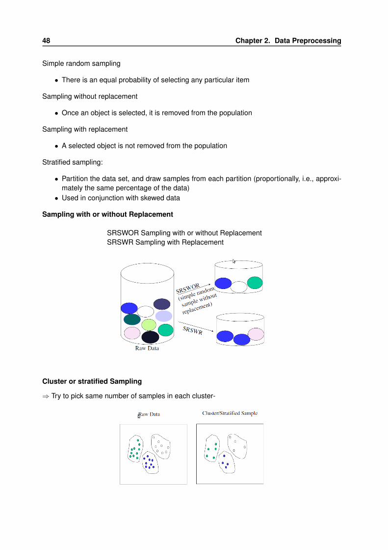
48 Chapter 2. Data Preprocessing
Simple random sampling
• There is an equal probability of selecting any particular item
Sampling without replacement
• Once an object is selected, it is removed from the population
Sampling with replacement
• A selected object is not removed from the population
Stratified sampling:
• Partition the data set, and draw samples from each partition (proportionally, i.e., approxi-mately the same percentage of the data)• Used in conjunction with skewed data
Sampling with or without Replacement
SRSWOR Sampling with or without ReplacementSRSWR Sampling with Replacement
Cluster or stratified Sampling
⇒ Try to pick same number of samples in each cluster-

2.4. Data Reduction 49
2.4.3.6 Data Cube agregation
• The lowest level of a data cube (base cuboid)
• The aggregated data for an individual entity of interest• E.g., a customer in a phone calling data warehouse
• Multiple levels of aggregation in data cubes
• Further reduce the size of data to deal with
• Reference appropriate levels
• Use the smallest representation which is enough to solve the task
• Queries regarding aggregated information should be answered using data cube, whenpossible
2.4.4 Data Compression
String compression:
• There are extensive theories and well-tuned algorithms• Typically lossless• But only limited manipulation is possible without expansion
Audio/video compression
• Typically lossy compression, with progressive refinement• Sometimes small fragments of signal can be reconstructed without reconstructing the
whole
Dimensionality and numerosity reduction may also be considered as forms of data

50 Chapter 2. Data Preprocessing
2.5 Data Transformation and data Discretization
2.5.1 Data Transformation
A function that maps the entire set of values of a given attribute to a new set of replacementvalues s.t. each old value can be identified with one of the new values
Methods :
Data Cleaning
• Smoothing: Remove noise from data
→ Seen in previous section 2.4.2
Data Reduction
• Attribute/feature construction→ New attributes constructed from the given ones• Aggregation: Summarization, data cube construction
→ Seen in previous section 2.4
Other transformations
• Normalization: Scaled to fall within a smaller, specified range
• min-max normalization• z-score normalization• normalization by decimal scaling
• Discretization: Concept hierarchy climbing
2.5.1.1 Normalization
Min-max normalization: to [new_minA, new_maxA]
ν ′ =ν −minA
maxA −minA(new_maxA − new_minA) + new_minA
Ex. Let income range $12,000 to $98,000 normalized to [0.0, 1.0]. Then $73,000 is mapped to
73600− 12000
98000− 12000(1.0− 0.0) + 0.0)0.716
New range runs from new_minA to new_maxA
Z-score normalization (µ: mean, σ: standard deviation):
ν ′ =ν − µAσA

2.5. Data Transformation and data Discretization 51
Ex. Let µ = 54,000, σ = 16,000. Then
73600− 54000
16000= 1.225
New range runs from −∞ to∞
Normalization by decimal scaling
ν ′ =ν
10j
where j is the smallest integer such that Max(|v′|) < 1
Ex. Suppose that the recorded values of A range from -986 to 917. The maximum absolutevalue of A is 986. To normalize by decimal scaling, we therefore divide each value by 1,000 (i.e.,j = 3) so that -986 normalizes to -0.986 and 917 normalizes to 0.917
New range runs from −1 to +1
2.5.2 Data Discretization
Three types of attributes :
• Nominal - values from an unordered set, e.g., color, profession• Ordinal - values from an ordered set, e.g., military or academic rank• Numeric - values: real numbers, e.g., integer or real numbers
Discretization: Divide the range of a continuous attribute into intervals
• Interval labels can then be used to replace actual data values• Reduce data size by discretization• Supervised vs. unsupervised• Split (top-down) vs. merge (bottom-up)• Discretization can be performed recursively on an attribute• Prepare for further analysis, e.g., classification
2.5.2.1 Data Discretization Methods
Typical methods: All the methods can be applied recursively
• Binning : Top-down split, unsupervised (Closed to what is done in data reduction but thistime applied to attributes)• Histogram analysis : Top-down split, unsupervised• Other Methods :
• Clustering analysis (unsupervised, top-down split or bottom-up merge)• Decision-tree analysis (supervised, top-down split)• Correlation (e.g. χ2) analysis (unsupervised, bottom-up merge)

52 Chapter 2. Data Preprocessing
2.5.2.2 Simple Discretization : Binning
Equal-width (distance) partitioning :
• Divides the range into N intervals of equal width (equals range size, uniform grid)• if A and B are the lowest and highest values of the attribute, the width of intervals will be:W = (B −A)/N .• The most straightforward, but outliers may dominate presentation• Skewed data is not handled well
Equal-depth (frequency) partitioning
• Divides the range into N intervals, each containing approximately same number of sam-ples• Good data scaling• Managing categorical attributes can be tricky
Examples :
Sorted data for price (in dollars): 4, 8, 9, 15, 21, 21, 24, 25, 26, 28, 29, 34
→ Partition into equal-frequency (equi-depth) bins:
• Bin 1: 4, 8, 9, 15• Bin 2: 21, 21, 24, 25• Bin 3: 26, 28, 29, 34
→ Smoothing by bin means:
• Bin 1: 9, 9, 9, 9• Bin 2: 23, 23, 23, 23• Bin 3: 29, 29, 29, 29
→ Smoothing by bin boundaries:
• Bin 1: 4, 4, 4, 15• Bin 2: 21, 21, 25, 25• Bin 3: 26, 26, 26, 34
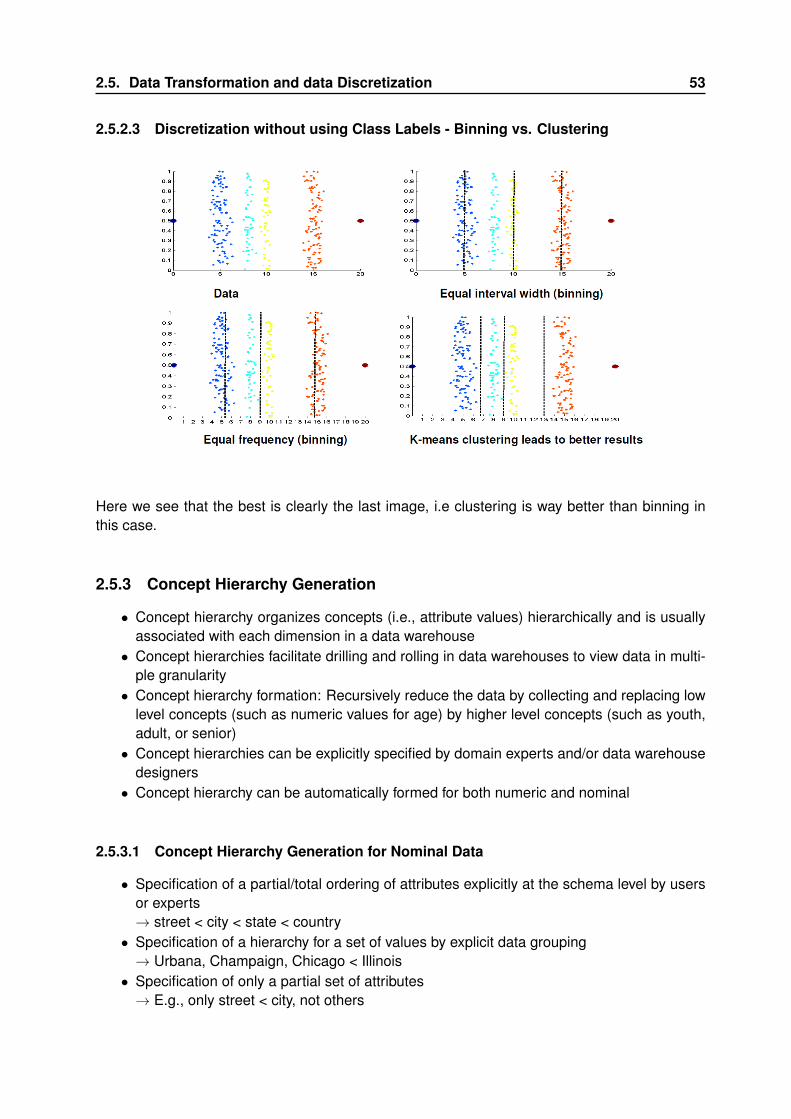
2.5. Data Transformation and data Discretization 53
2.5.2.3 Discretization without using Class Labels - Binning vs. Clustering
Here we see that the best is clearly the last image, i.e clustering is way better than binning inthis case.
2.5.3 Concept Hierarchy Generation
• Concept hierarchy organizes concepts (i.e., attribute values) hierarchically and is usuallyassociated with each dimension in a data warehouse• Concept hierarchies facilitate drilling and rolling in data warehouses to view data in multi-
ple granularity• Concept hierarchy formation: Recursively reduce the data by collecting and replacing low
level concepts (such as numeric values for age) by higher level concepts (such as youth,adult, or senior)• Concept hierarchies can be explicitly specified by domain experts and/or data warehouse
designers• Concept hierarchy can be automatically formed for both numeric and nominal
2.5.3.1 Concept Hierarchy Generation for Nominal Data
• Specification of a partial/total ordering of attributes explicitly at the schema level by usersor experts→ street < city < state < country• Specification of a hierarchy for a set of values by explicit data grouping→ Urbana, Champaign, Chicago < Illinois• Specification of only a partial set of attributes→ E.g., only street < city, not others

54 Chapter 2. Data Preprocessing
• Automatic generation of hierarchies (or attribute levels) by the analysis of the number ofdistinct values→ E.g., for a set of attributes: street, city, state, country
2.5.3.2 Automatic Concept Hierarchy Generation
Some hierarchies can be automatically generated based on the analysis of the number of distinctvalues per attribute in the data set
• The attribute with the most distinct values is placed at the lowest level of the hierarchy• Exceptions, e.g., weekday, month, quarter, year
2.6 Practice
2.6.1 Computation on Data
Suppose that the data for analysis includes the attribute age. The age values for the data tuplesare (in increasing order) 13, 15, 16, 16, 19, 20, 20, 21, 22, 22, 25, 25, 25, 25, 30, 33, 33, 35, 35,35, 35, 36, 40, 45, 46, 52, 70.
2.6.1.1 mean / median
What is the mean of the data ? What is the median?
Remainder :
• odd number of values : take middle values• even number of values : take mean of both middle values
The (arithmetic) mean of the data is approx 30.The median (middle value of the ordered set, as the number of values in the set is odd) of thedata is: 25.

2.6. Practice 55
2.6.1.2 mode
What is the mode of the data? Comment on the data’s modality (i.e., bimodal, trimodal, etc.).
Remainder :
1. find the value occuring at the highest frequency, count the very highest frequency2. count the number of different values occuring at this very highest frequency
This data set has two values that occur with the same highest frequency and is, therefore,bimodal.The modes (values occurring with the greatest frequency) of the data are 25 and 35.
2.6.1.3 midrange
What is the midrange of the data?
Remainder :
• The midrange is the average of the largest and smallest values in the data set
The midrange of the data is: (70 + 13)/2 = 41.5
2.6.1.4 quartile
Can you find (roughly) the first quartile (Q1) and the third quartile (Q3) of the data?
The first quartile (corresponding to the 25th percentile) of the data is: 20. The third quartile(corresponding to the 75th percentile) of the data is: 35.
2.6.1.5 5-numbers summary
Give the five-number summary of the data (the minimum value, first quartile, median value, thirdquartile, and maximum value)
The five number summary of a distribution consists of the minimum value, first quartile, medianvalue, third quartile, and maximum value. It provides a good summary of the shape of thedistribution and for this data is: 13, 20, 25, 35, 70.
2.6.1.6 boxplot
Show a boxplot of the data.

56 Chapter 2. Data Preprocessing
2.6.2 Smoothing
Suppose that the data for analysis includes the attribute age. The age values for the data tuplesare (in increasing order) 13, 15, 16, 16, 19, 20, 20, 21, 22, 22, 25, 25, 25, 25, 30, 33, 33, 35, 35,35, 35, 36, 40, 45, 46, 52, 70.
2.6.2.1 Smoothing by bin means
Use smoothing by bin means to smooth the above data, using a bin depth of 3. Illustrate yoursteps.
The following steps are required to smooth the above data using smoothing by bin meanswith a bin depth of 3.
Step 1: Sort the data. (This step is not required here as the data are already sorted.)
Step 2: Partition the data into equal-frequency bins of size 3.
Bin 1: 13, 15, 16Bin 2: 16, 19, 20Bin 3: 20, 21, 22Bin 4: 22, 25, 25Bin 5: 25, 25, 30Bin 6: 33, 33, 35Bin 7: 35, 35, 35Bin 8: 36, 40, 45Bin 9: 46, 52, 70
Step 3: Calculate the arithmetic mean of each bin.
Replace each of the values in each bin by the arithmetic mean calculated for the bin.
Bin 1: 14.7 14.7 14.7Bin 2: 18.33 18.33 18.33

2.6. Practice 57
Bin 3: 21, 21, 21Bin 4: 24, 24, 24Bin 5: 26.7 26.7 26.7Bin 6: 33.7 33.7 33.7Bin 7: 35, 35, 35Bin 8: 40.3 40.3 40.3Bin 9: 56, 56, 56
2.6.2.2 Outliers
How might you determine outliers in the data?
Outliers in the data may be detected by clustering, where similar values are organized intogroups, or "clusters". Values that fall outside of the set of clusters may be considered outliers.Alternatively, a combination of computer and human inspection can be used where a predeter-mined data distribution is implemented to allow the computer to identify possible outliers. Thesepossible outliers can then be verified by human inspection with much less effort than would berequired to verify the entire initial data set.
2.6.2.3 Data smoothing
What other methods are there for data smoothing?
Other methods that can be used for data smoothing include alternate forms of binning suchas smoothing by bin medians or smoothing by bin boundaries. Alternatively, equal-width binscan be used to implement any of the forms of binning, where the interval range of values ineach bin is constant. Methods other than binning include using regression techniques to smooththe data by fitting it to a function such as through linear or multiple regression. Classificationtechniques can be used to implement concept hierarchies that can smooth the data by rolling-uplower level concepts to higher-level concepts.
2.6.3 Data Reduction and tranformation
Suppose a hospital tested the age and body fat data for 18 randomly selected adults with thefollowing result:
age 23 23 27 27 39 41 47 49 50%fat 9.5 26.5 7.8 17.8 31.4 25.9 27.4 27.2 31.2age 52 54 54 56 57 58 58 60 61%fat 34.6 42.5 28.8 33.4 30.2 34.1 32.9 41.2 35.7

58 Chapter 2. Data Preprocessing
2.6.3.1 Computation on data
Calculate the mean, median and standard deviation of age and %fat.
For the variable age the mean is 46.44, the median is 51, and the standard deviation is 12.85.For the variable %fat the mean is 28.78, the median is 30.7, and the standard deviation is 8.99.
2.6.3.2 Boxplot
Draw the boxplots for age and %fat.
2.6.3.3 z-scores normalization
Normalize the two variables based on z-score normalization.
Remainder ZA = vA−µAσA
age 23 23 27 27 39 41 47 49 50z-age -1.83 -1.83 -1.51 -1.51 -0.58 -0.42 -0.04 0.20 0.28%fat 9.5 26.5 7.8 17.8 31.4 25.9 27.4 27.2 31.2z-fat -2.14 -0.25 -2.33 -1.22 -0.29 -0.32 -0.15 -0.18 0.27age 52 54 54 56 57 58 58 60 61z-age 0.43 0.59 0.59 0.74 0.82 0.90 0.90 1.06 1.13%fat 34.6 42.5 28.8 33.4 30.2 34.1 32.9 41.2 35.7z-fat 0.65 1.53 0.0 0.51 0.16 0.59 0.56 1.38 0.77
2.6.3.4 Correlation coefficient
Calculate the correlation coefficient (Pearson’s product moment coefficient). Are these two vari-ables positively or negatively correlated?
The correlation coefficient is 0.82. The variables are positively correlated.

2.6. Practice 59
2.6.4 Sampling
Suppose that the data for analysis includes the attribute age. The age values for the data tuplesare (in increasing order) 13, 15, 16, 16, 19, 20, 20, 21, 22, 22, 25, 25, 25, 25, 30, 33, 33, 35, 35,35, 35, 36, 40, 45, 46, 52, 70.
2.6.4.1 Equal-width histogram
Plot an equal-width histogram of width 10.
2.6.4.2 Sampling
Sketch examples of each of the following sampling techniques: SRSWOR, SRSWR, clustersampling, stratified sampling.Use samples of size 5 and the strata “young", “middle-age", and ”senior".

60 Chapter 2. Data Preprocessing

CHAPTER 3
An introduction to Data Mining
Contents3.1 Why Data Mining ? . . . . . . . . . . . . . . . . . . . . . . . . . . . . . . . . . . . . 59
3.1.1 Information is crucial . . . . . . . . . . . . . . . . . . . . . . . . . . . . . . . . 59
3.2 What is Mining ? . . . . . . . . . . . . . . . . . . . . . . . . . . . . . . . . . . . . . 603.2.1 Knowledge Discovery (KDD) Process . . . . . . . . . . . . . . . . . . . . . . 60
3.2.2 Data mining in Business Intelligence . . . . . . . . . . . . . . . . . . . . . . . 61
3.2.3 Data mining : confluence of multiple disciplines . . . . . . . . . . . . . . . . . 61
3.3 Data mining functions . . . . . . . . . . . . . . . . . . . . . . . . . . . . . . . . . . 623.3.1 Generalization . . . . . . . . . . . . . . . . . . . . . . . . . . . . . . . . . . . 62
3.3.2 Association and Correlation Analysis . . . . . . . . . . . . . . . . . . . . . . . 62
3.3.3 Classification . . . . . . . . . . . . . . . . . . . . . . . . . . . . . . . . . . . . 62
3.3.4 Cluster Analysis . . . . . . . . . . . . . . . . . . . . . . . . . . . . . . . . . . 63
3.3.5 Outlier analysis . . . . . . . . . . . . . . . . . . . . . . . . . . . . . . . . . . . 63
3.4 Evaluation of Knowledge . . . . . . . . . . . . . . . . . . . . . . . . . . . . . . . . 633.5 Practice . . . . . . . . . . . . . . . . . . . . . . . . . . . . . . . . . . . . . . . . . . . 63
3.1 Why Data Mining ?
The Explosive Growth of Data: from terabytes to petabytes
→ Data collection and availability :
• Automated data collection tools, database systems, Web, computerized society
→ Major sources of abundant data
• Business: Web, e-commerce, transactions, stocks, ...• Science: Remote sensing, bioinformatics, scientific simulation, ...• Society and everyone: news, digital cameras, YouTube
→We are drowning in data, but starving for knowledge!
→ "Necessity is the mother of invention"→ Data mining→ Automated analysis of massive datasets
Raw data is useless: need techniques to automatically extract information from it

62 Chapter 3. An introduction to Data Mining
• Data: recorded facts• Information: patterns underlying the data
3.1.1 Information is crucial
Example 1: in vitro fertilization
• Given: embryos described by 60 features• Problem: selection of embryos that will survive• Data: historical records of embryos and outcome
Example 2: cow culling
• Given: cows described by 700 features• Problem: selection of cows that should be culled• Data: historical records and farmer’s decisions
3.2 What is Mining ?
Data mining (knowledge discovery from data) :
• Extraction of interesting (non-trivial, implicit, previously unknown and potentially useful)patterns or knowledge from huge amount of data• Data mining: a misnomer?
Alternative names :
• Knowledge discovery (mining) in databases (KDD), knowledge extraction, data/patternanalysis, data archeology, data dredging, information harvesting, business intelligence,etc.
Watch out: Is everything “data mining”?
• Simple search and query processing• (Deductive) expert systems
3.2.1 Knowledge Discovery (KDD) Process
Below is a view from typical database systems and data warehousing communities.Data miningplays an essential role in the knowledge discovery process :

3.2. What is Mining ? 63
3.2.2 Data mining in Business Intelligence
3.2.3 Data mining : confluence of multiple disciplines

64 Chapter 3. An introduction to Data Mining
→ Tremendous amount of data :
• Algorithms must be highly scalable to handle such as terabytes of data
→ High-dimensionality of data :
• Micro-array may have tens of thousands of dimensions
→ High complexity of data :
• Data streams and sensor data• Time-series data, temporal data, sequence data• Structure data, graphs, social networks and multi-linked data• Heterogeneous databases and legacy databases• Spatial, spatiotemporal, multimedia, text and Web data• Software programs, scientific simulations
→ New and sophisticated applications
3.3 Data mining functions
3.3.1 Generalization
→ Information integration and data warehouse construction :
• Data cleaning, transformation, integration, and multidimensional data model
→ Data cube technology :
• Scalable methods for computing (i.e., materializing) multidimensional aggregates• OLAP (online analytical processing)
→ Multidimensional concept description: Characterization and discrimination :
• Generalize, summarize, and contrast data characteristics, e.g., dry vs. wet region
3.3.2 Association and Correlation Analysis
→ Frequent patterns (or frequent itemsets)
• What items are frequently purchased together in your Walmart?
→ Association, correlation vs. causality
• A typical association rule : Diaper→ Beer [0.5%, 75%] (support, confidence)• Are strongly associated items also strongly correlated?
→ How to mine such patterns and rules efficiently in large datasets?
→ How to use such patterns for classification, clustering, and other applications?

3.4. Evaluation of Knowledge 65
3.3.3 Classification
→ Classification and label prediction
• Construct models (functions) based on some training examples• Describe and distinguish classes or concepts for future prediction. E.g., classify countries
based on (climate), or classify cars based on (gas mileage)• Predict some unknown class labels
→ Typical methods
• Decision trees, naïve Bayesian classification, support vector machines, neural networks,rule-based classification, pattern-based classification, logistic regression, ...
→ Typical applications:
• Credit card fraud detection, direct marketing, classifying stars, diseases, web-pages, ...
3.3.4 Cluster Analysis
• Unsupervised learning (i.e., Class label is unknown)• Group data to form new categories (i.e., clusters), e.g., cluster houses to find distribution
patterns• Principle: Maximizing intra-class similarity & minimizing interclass similarity• Many methods and applications
3.3.5 Outlier analysis
• Outlier: A data object that does not comply with the general behavior of the data• Noise or exception? - One person’s garbage could be another person’s treasure• Methods: by product of clustering or regression analysis, ...• Useful in fraud detection, rare events analysis
3.4 Evaluation of Knowledge
Are all mined knowledge interesting?
• One can mine tremendous amount of "patterns" and knowledge• Some may fit only certain dimension space (time, location, ...)• Some may not be representative, may be transient, ...
Evaluation of mined knowledge→ directly mine only interesting knowledge?
• Descriptive vs. predictive• Coverage• Typicality vs. novelty

66 Chapter 3. An introduction to Data Mining
• Accuracy• Timeliness
3.5 Practice
Define the data mining tasks and give an example for each of them:
Generalization:
Generalization consists of data cleaning, transformation, integration, aggregation and/orsummarization.
For instance one might want to replace the age attribute of some data by a category such asyoung, middle aged or old.
Association and Correlation Analysis:
This is typically finding association between data enabling one to deduce rules such as "ifone buys beer then he watches footbal on TV" or find closely related attributes sur as play_chessand read_books.
Classification:
Classification is about constructing models or distinguishing classes or concepts for futureprediction.
For instance one might want to classify countries based on (climate), or classify cars basedon (gas mileage)
Cluster Analysis:
Cluster analysis is about building clusters to form categories or for data reduction.
For instance one might want to cluster houses to find distribution patterns.
Outlier analysis:
Outlier analysis is about finding objects that does not comply with the general behavior ofthe data. It is for instance used in fraud detection or rare event analysis.

CHAPTER 4
Market Basket Analysis
Contents4.1 Motivation . . . . . . . . . . . . . . . . . . . . . . . . . . . . . . . . . . . . . . . . . 65
4.2 Market Basket Analysis : MBA . . . . . . . . . . . . . . . . . . . . . . . . . . . . . 65
4.2.1 Usefulness of MBA . . . . . . . . . . . . . . . . . . . . . . . . . . . . . . . . . 66
4.3 Association rule . . . . . . . . . . . . . . . . . . . . . . . . . . . . . . . . . . . . . . 66
4.3.1 Formalisation of the problem . . . . . . . . . . . . . . . . . . . . . . . . . . . 66
4.3.2 Association rule - definition . . . . . . . . . . . . . . . . . . . . . . . . . . . . 67
4.3.3 Example . . . . . . . . . . . . . . . . . . . . . . . . . . . . . . . . . . . . . . . 67
4.3.4 Measure of the Support . . . . . . . . . . . . . . . . . . . . . . . . . . . . . . 67
4.3.5 Measure of the Confidence . . . . . . . . . . . . . . . . . . . . . . . . . . . . 68
4.3.6 Support and confidence . . . . . . . . . . . . . . . . . . . . . . . . . . . . . . 68
4.3.7 Interesting rules . . . . . . . . . . . . . . . . . . . . . . . . . . . . . . . . . . 68
4.3.8 Lift . . . . . . . . . . . . . . . . . . . . . . . . . . . . . . . . . . . . . . . . . . 69
4.3.9 Dissociation rules . . . . . . . . . . . . . . . . . . . . . . . . . . . . . . . . . 70
4.3.10 The co-events table . . . . . . . . . . . . . . . . . . . . . . . . . . . . . . . . 70
4.4 MBA : The base process . . . . . . . . . . . . . . . . . . . . . . . . . . . . . . . . . 70
4.4.1 Choose the right set of article . . . . . . . . . . . . . . . . . . . . . . . . . . . 70
4.4.2 Anonymity↔ nominated . . . . . . . . . . . . . . . . . . . . . . . . . . . . . . 71
4.4.3 Notation / Vocabulary . . . . . . . . . . . . . . . . . . . . . . . . . . . . . . . 71
4.5 Rule extraction algorithm . . . . . . . . . . . . . . . . . . . . . . . . . . . . . . . . 71
4.5.1 First phase : Compute frequent article subsets . . . . . . . . . . . . . . . . . 71
4.5.2 Constraints . . . . . . . . . . . . . . . . . . . . . . . . . . . . . . . . . . . . . 75
4.5.3 Second phase : Compute interesting rules . . . . . . . . . . . . . . . . . . . 76
4.6 Partitionning . . . . . . . . . . . . . . . . . . . . . . . . . . . . . . . . . . . . . . . . 77
4.6.1 Algorithm . . . . . . . . . . . . . . . . . . . . . . . . . . . . . . . . . . . . . . 77
4.7 Conclusion . . . . . . . . . . . . . . . . . . . . . . . . . . . . . . . . . . . . . . . . . 77
4.8 Practice . . . . . . . . . . . . . . . . . . . . . . . . . . . . . . . . . . . . . . . . . . . 78
4.8.1 support and confidence . . . . . . . . . . . . . . . . . . . . . . . . . . . . . . 78
4.8.2 apriori . . . . . . . . . . . . . . . . . . . . . . . . . . . . . . . . . . . . . . . . 81

68 Chapter 4. Market Basket Analysis
4.1 Motivation
Example :
• Where to place laundry products in order to optimize sales?• Does one also buy butter when on buys milk?• Is sugar likely to be also sold when one buys bread and
milk at the same time?
→ Sales information : who ? what ? why ?
• Most sales organisms encounter decision-making tool.• Bar code technologies enables sales organisms to collect huge and massive amount of
sales data "market basket data".• Those organisms are interested in analyzing those data to extract informations aimed at
helping marketing to develop and apply commercial programs and strategies adapted tothe client needs.
4.2 Market Basket Analysis : MBA
MBA is a technic enabling to find the list of articles having a tendency to be sold together upona client transaction.
• The transaction data is available• The groups of articles we are looking for are unknown before the analysis• → Undirected Data-Mining
We try to build a model built on conditional rules :
• If condition then result• Several conditions can be combined to obtain the result : If A and B then C• Several logical operators can be combined : If A and not B then C
4.2.1 Usefulness of MBA
MBA’s result is a set of association rules :
useful and clear rules :
• Association rule : simple rules : " If condition then result "Ex : if a client buys butter, the he buys milk too.Ex : if a client buys milk and salt, the he buys cheese too.
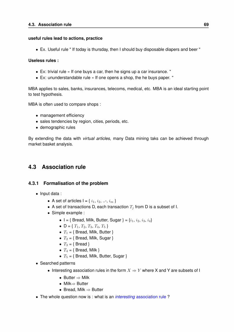
4.3. Association rule 69
useful rules lead to actions, practice
• Ex. Useful rule " If today is thursday, then I should buy disposable diapers and beer "
Useless rules :
• Ex: trivial rule « If one buys a car, then he signs up a car insurance. "• Ex: ununderstandable rule « If one opens a shop, the he buys paper. "
MBA applies to sales, banks, insurances, telecoms, medical, etc. MBA is an ideal starting pointto test hypothesis.
MBA is often used to compare shops :
• management efficiency• sales tendencies by region, cities, periods, etc.• demographic rules
By extending the data with virtual articles, many Data mining taks can be achieved throughmarket basket analysis.
4.3 Association rule
4.3.1 Formalisation of the problem
• Input data :
• A set of articles I = { i1, i2, ..-, im }• A set of transactions D, each transaction Tj from D is a subset of I.• Simple example :
• I = { Bread, Milk, Butter, Sugar } = {i1, i2, i3, i4}• D = { T1, T2, T3, T4, T5 }• T1 = { Bread, Milk, Butter }• T2 = { Bread, Milk, Sugar }• T3 = { Bread }• T4 = { Bread, Milk }• T5 = { Bread, Milk, Butter, Sugar }
• Searched patterns
• Interesting association rules in the form X ⇒ Y where X and Y are subsets of I
• Butter⇒ Milk• Milk⇒ Butter• Bread, Milk⇒ Butter
• The whole question now is : what is an interesting association rule ?

70 Chapter 4. Market Basket Analysis
4.3.2 Association rule - definition
• Let I be a a set of articles• Let D be a set of transactions, each transaction Tj is a set of articles from I• An association rule is an implication of the form X ⇒ Y where X ⊂ I and Y ⊂ I andX ∩ Y = ∅
4.3.3 Example
This is the example we will be focusing on in the rest of this document
I = { Bread, Milk, Butter, Sugar }
Tran. ID Articles listT1 Bread, Milk, ButterT2 Bread, Milk, SugarT3 BreadT4 Bread, MilkT5 Bread, Milk, Butter, Sugar
4.3.4 Measure of the Support
Definition : The support of the association rule X ⇒ Y in the base D represents the ratiobetween the number of transactions in the base D where both X and Y appear and the totalnumber of number transactions.
Sup(X ⇒ Y,D) = |{T ∈ D,T ⊃ X ∪ Y }|/|D| = P (X ∪ Y )
Notation issue : Sup(X ⇒ Y ) is sometimes noted Sup(X,Y) and Sup (X,Y ⇒ Z) is sometimesnoted Sup(X,Y,Z) in the rest of this document.
Example (using example 4.3.3) :
• Sup(Bread, Milk) = 4 / 5 = 0.8 = 80%

4.3. Association rule 71
• Sup(Bread, Milk, Sugar) = 2 / 5 = 0.4 = 40%
Note: We also speak of support when considerating a single article: Sup(Milk) = 4 / 5 = 0.8= 80%
4.3.5 Measure of the Confidence
Definition : The confidence of the association rule X ⇒ Y in the base D represents the ratiobetween the number of transactions in the base D where both X and Y appear and the numberof number transactions where only X appear.
Conf(X ⇒ Y,D) = Sup(X ⇒ Y,D)/Sup(X,D) = P (Y |X)
(where D is the set of transactions)
Other notation (without any mention to D the set of transactions)
Conf(X,Y ⇒ Z) = Sup(X,Y, Z)/Sup(X,Y ) = P (Z|(XandY ))
Example (using example 4.3.3) :
• Conf(Bread⇒ Milk) = 4 / 5 = 0.8 = 80%• Conf(Bread, Milk⇒ Suggar) = 2 / 4 = 0.5 = 50%
4.3.6 Support and confidence
• support ( X⇒ Y ) = P ( X and Y ) = support ( Y⇒ X )
• Note : however we will always consider lexicographical order. Hence we have tosort the article set, transactions, etc.
• confidence ( X⇒ Y ) = P ( Y | X ) = P ( X and Y ) / P ( X )• support and confidence represent propabilities• sup, conf ∈ [0, 1]
4.3.7 Interesting rules
Definition : Given two threshold values fixed a priori by some user :
• a minimal support threshold value "minsup" and• a minimal confidence threshold value "minconf" and
A rule X ⇒ Y is interesting within D if and only if
• Sup(X⇒ Y, D) ≥ minsup• Conf(X⇒ Y, D) ≥ minconf
The whole purpose of Market Basket Analysis is to spot out every interesting rule given thetwo threshold values "minsup" and "minconf".

72 Chapter 4. Market Basket Analysis
Example (using example 4.3.3) :
Let’s assume minsup = 2/5 and minconf = 3/4.
• {Milk, Butter, Sugar⇒ Bread}: not interesting→ Conf = 1 / 1 ≥ minconf but Sup = 1 / 5 < minsup• {Bread, Milk⇒ Butter}: not interesting→ Sup = 2 / 5 ≥ minsup but Conf = 2 / 4 < minconf• {Milk, Butter⇒ Bread}: interesting→ Sup = 2 / 5 ≥ minsup and Conf = 2 / 2 ≥ minconf
4.3.8 Lift
Definition : The lift (interest, amelioration, correlation) of the rule { condition⇒ result } is definedby the ratio between the confidence of the rule and the support of the result.
Lift(condition⇒ result) = Conf(condition and result)/Sup(result)
Lift(condition⇒ result) = P (condition and result)/(P (condition) ∗ P (result))
• If the the lift is > 1, then the rule "condition⇒ result" is better for the prediction than simplyguessing the result.• If the the lift is ≤ 1, then guessing the result is simply better.• Note: If P(condition and result) = P(condition) * P(result) Then (⇒) condition and result
are independent.
Example :
Let A, B, C be three articles :
• P(A)=45% =Sup(A)• P(B)=42.5% =Sup(B)• P(C)=40 =Sup(C)• P(A and B)=25% =Sup(A and B)• P(A and C)=20% =Sup(A and C)• P(B and C)=15% =Sup(B and C)• P(A and B and C)=5% =Sup(A and B and C)
Rule P(cond.) P(cond. and res.) P(res.) Confidence liftComputat. (given) P(A and B and C) (given) P(cond. and res.)
/ P(cond)P(cond. and res.)/(P(cnd.)*P(res))
A,B⇒ C 0.25 0.05 0.4 0.05 / 0.25 = 0.2 0.05 / (0.25 * 0.4)A,C⇒ B 0.2 0.05 0.425 0.05 / 0.2 = 0.25 0.05 / (0.2 * 0.425)B,C⇒ A 0.15 0.05 0.45 0.05 / 0.15 = 0.33 0.05 / (0.15 * 0.44)
4.3.9 Dissociation rules
A dissociation rule is quite similar to an association rule except it can contain the not operator :

4.4. MBA : The base process 73
If A and not B then C
They are generated using exactly the same algorithm. For this to work, a new set of articlesis added to the article set.
A, B, C→ not-A, not-B, not-C
Problems :
• The number of article doubles, so the performance decreases• the frequency of the not-X tends to be much higher than the frequency of the usual articles→ If not-A and not-B then not-C (pretty much useless)
4.3.10 The co-events table
It is sometimes useful to put events in a table in order to compute in one singe place the supportand / or confidence for ever possible rule
2D table : column gives X , row gives X - type in each cell conf(X⇒Y) and use the array inconjuction with a minimum confidence to decide which rules are worth investigating.
Can be generalized in the very same principle to nD tables (n dimensions).
4.4 MBA : The base process
1. Choose the right set of article
2. Create rules by using the co-events table
3. Lower complexity by using tresholds values (i.e. everything below is not taken into ac-count).
4.4.1 Choose the right set of article
We have the details of transaction and hierarchies. So we can :
agregate : { red apple, green apple, yellow apple } = {apple}
generalize :
• for instance by using taxonomies• Caution: choose the "right" level of generalization.

74 Chapter 4. Market Basket Analysis
4.4.2 Anonymity↔ nominated
Client transaction are anonym in general.
However the usage of credit cards or fidelity cards enables the sales departement to knowabout clients, their habits, etc. This enables the tracking ot the various kinds of behavioursacross time.
4.4.3 Notation / Vocabulary
• A set of articles is called an itemset• a set of k articles is called a k-itemset• a k-itemset which satisfies the minsup (minimal support) criteria is called a frequent k-
itemset
4.5 Rule extraction algorithm
The rule extraction algorithm is called Apriori. It consists of two principal phases :
1. Computation of all frequent article sub-sets X→ Search of all the frequent sub-sets X of I, i.e those respecting Sup (X , D) ≥ minsup
2. Computation of all the interesting association rules (X - Y⇒ Y )Note : X and Y are article sets. Hence a rule of the form (X - Y⇒ Y ), if X = {A, B, C} andY = {C} is a well know association rule form : ( A,B⇒ C )→ A partir des sous-ensembles X fréquents déterminés lors de la première phase, cal-culer toutes les règles de confiances suffisantes, c.a.d. les règles d’association telles queConf(X -Y⇒ Y / D) ≥ minconf
Note :
X - Y⇒ Y can be noted X / Y⇒ Y, it’s exactly the same. The two notations are equivalent.
4.5.1 First phase : Compute frequent article subsets
Base principle :
• Base on the support computation fundamental property : If X ⊆ Y, then Sup(X , D) ≥Sup(Y , D) for all D• Any subset of a frequent itsemset is frequent• any sur-set of a non-frequent itemset is not frequent
Ascending search of frequent itsemsets :
• Stage 1 : compute frequent 1-itemsets = frequent subsets of I containing only 1 article• Stage k : compute frequent k-itemsets from the (k-1)-itemsets = frequent subsets of I
containing only k articles

4.5. Rule extraction algorithm 75
4.5.1.1 The Apriori algorithm (1st phase)
• Input :
• A set D of transactions Ti• minsup
• Output :
• A set L of all frequent itemsets
• Method :
• Compute the set L(1) of frequent 1-itemsets• Let K = 2• While L(K-1) is not empty (L(K-1) = result from the previous iteration)
• // Stage 1.a : candidates generationCompute the set C(K) of the K-itemsets candidate from L(K-1) (see below)• // Stage 1.b : candidates evaluation→ Compute the support for each candidate C in C(K)→ Let L(K) be the set of candidates C from C(K) such that Sup(C,D) ≥ min-sup. L(K) is the set of all frequent K-itemsets.• K = K + 1
candidates generation :
• Input :
• A set L(K-1) of the frequent (K-1)-itemsets
• Output :
• A set C(K) of the K-itemsets candidates
• Method :
• (join or composition phase)Built C(K) the set of K-itemsets C :
• C = F1 ∪ F2 where F1 and F2 are elements of L(K-1)• F1 ∩ F2 contains K-2 elements
• (pruning phase [FR : élagage])Remove from C(K) any candidate C if there is
• a subset of C of (K-1) elements not present in L(K-1)
• Return C(K)
Note : the candidate generation occurs in memory without accessing the data.
candidates evaluation :
• Input :
• A set C(K) of the candidates K-itemsets• The set of transactions D• minsup
• Output :

76 Chapter 4. Market Basket Analysis
• A set L(K) of the frequent K-itemsets
• Method :
• Initialize L(K) to the empty set• Count the number of occurence of every candidate of C(K) in D
For every candidate of C(K),
• For every transaction Ti of D : if C is included in Ti, then C.Sup += 1• id C.Sup ≥ minsup, then add C to L(K)
• Return L(K)
Note : the evaluation of the candidates occurs in one single pass on the data.
4.5.1.2 Example
Computation of L(1)
• T1 = { Pain, Lait, Beurre },• T2 = { Pain, Lait, Sucre },• T3 = { Pain },• T4 = { Pain, Lait }• T5 = { Pain, Lait, Beurre, Sucre }• Minsup = 2/5
Generation of C(2)
• Composition of the L(1) elements : two-by-two union• Pruning of the candidates : none at this level
Evaluation of C(2)

4.5. Rule extraction algorithm 77
The computation of L(2) occurs in one single pass on the data.
Generation of C(3)
The composition of the elements from C(3) happens by composing withthe elements fromL(2). Only the itemsets having the same first elements are combined
Pruning the elements from C(3) : The candidates {Bread, Sugar, Butter} and {Milk, Sugar,Butter } are removed from C3 as {Sugar, Butter} is not present in L(2) :
Evaluation of C(3) : straightforward
Generation of C(4)
Composition des éléments de L(3) :

78 Chapter 4. Market Basket Analysis
Pruning the elements from C(4) : {Bread, Milk, Sugar, Butter} is removed as {Milk, Sugar,Butter} is not present in L(3). C(4) is hence empty and so is L(4)
End of the frequent itemset calculation :
4.5.2 Constraints
• Every transaction T should be sorted by ascending order (lexicographical order or anythingelse)• Every set L(k) should be sorted in ascending order.• Every frequentr k-itsemset should be sorted in ascending order.
4.5.2.1 Another exemple - starting from level 3
• Let L(3) = { {1, 2, 3}, {1, 2, 4}, {1, 3, 4}, {1, 3, 5}, {2, 3, 4} }• The join phase for C(4) :
• {1, 2, 3} is joined to {1, 2, 4} to produce {1, 2, 3, 4}• {1, 3, 4} is joined to {1, 3, 5} to produce {1, 3, 4, 5}• After the join, C4 ={{1, 2, 3, 4}, {1, 3, 4, 5}}
• In the pruning stage :
• For {1, 2, 3, 4} one should test the existence within L(3) of every 3-itemset, so {1,2,3}; {1, 2, 4}; {1, 3, 4}; {2, 3, 4}⇒ OK

4.5. Rule extraction algorithm 79
• For {1, 3, 4, 5} one tests {1, 3, 4}; {1, 3, 5}; {1, 4, 5}; {3, 4, 5}; As {1, 4, 5} is notfound in L3, {1, 3, 4, 5} is pruned
• Only {1, 2, 3, 4} stays in C4• The one still needs to compute the support and get rid of the 4-itemsets with a support
below minsup to build L(4)
4.5.3 Second phase : Compute interesting rules
4.5.3.1 The principle (naive method)
• For every k-itemset X frequent (with K > 1)
• For every possible Y ⊂ X
• Compute the confidence in the rule X - Y⇒ Y• If that confidence is greater than minconf, then the generated association rule
is interesting.
In other words :
• For every frequent itemset l, we find every subset of l different from the empty set.• For each of these subsets a, we generate the rule a ⇒ (l - a) if the ratio between the
support of l and the support of a is at least as big as minconf.
Note this phase doesn’t require any access to the data.
4.5.3.2 Example
Looking back at the 4.5.1.2 for the stage 1 of apriori shown before, when using minconf = 3 / 4and X = {Bread, Milk, Butter} is frequent :
• { Bread, Milk => Butter } not interesting because Conf = 2 / 4• { Bread, Butter => Milk } interesting because Conf = 2 / 2• { Milk, Butter => Bread } interesting because Conf = 2 / 2• { Bread => Milk, Butter } not interesting because Conf = 2 / 5• { Milk => Bread, Butter } not interesting because Conf = 2 / 4• { Butter => Bread, Milk } not interesting because Conf = 2 / 4
4.5.3.3 Optimize-it
• We can quite effectively optimize the procedure by generating the subsets of a frequentitemset in a recursive fashion.• For instance, for a given itemset {A,B,C,D}, we will first consider the subset {A,B,C}, then
{A,B}, etc.• Whenever a subset a of a frequent itemset l doesn’t generate any valable rule, the subsets
of a are not considered to generate rule from l.

80 Chapter 4. Market Basket Analysis
• For instance if {A,B,C} ⇒ D doesn’t have a sufficient confidence, one doesn’t need tocontrol whether {A,B}⇒ {C,D} is valable
A typical implementation for this consists of using a HashTree. The lecture support providesan extended discussion on this implementation but this resume won’t dig it any further.
4.6 Partitionning
The principle :
• Divide the set of transactions in a list of subsets : D1, D2, ...,Dp
• Apply apriori to each subset of the transactions• Every frequent itemset must be frequent in at least one subset of the transactions
4.6.1 Algorithm
• Divide D in D1, D2, ..., Dp;• For i = 1 to p do
• Li = Apriori ( Di );
• C = L1 ∪ ... ∪ Lp;• To Generate L, evaludate candidates on D;
Advantages :
• Adapts to the available amount of memory• easily parallelizable• the amount of scans of D is 2
Drawbacks :
• Might have a lof of condidates to analyze in phase 2
4.7 Conclusion
Perspectives:
• One might want to use other measures of interest that support and confidence→ Convic-tion, implication strength, etc.
Generalization of the association rules
• Taking numerical data into consideration• Taking hierarchies of attribute into consideration• Taking several tables into consideration• etc.

4.8. Practice 81
4.8 Practice
4.8.1 support and confidence
The Apriori algorithm uses prior knowledge of subset support properties.
4.8.1.1 support
Prove that all nonempty subsets of a frequent itemset must also be frequent:
• Let s be a frequent itemset• Let s’ be a subset of s• Let minsup be the minimum support• Let D be the set of database transaction (relevant data) and |D| the number of transactions
in D
Let’s assume that it’s not the case :
s is frequent⇒ sup(s) ≥ minsup
where sup(s) =count(s) in D
|D|s is frequent⇒ count(s) in D ≥ minsup ∗ |D|
But :
s′ is NOT frequent⇒ sup(s′) < minsup
where sup(s′) =count(s′) in D
|D|s′ is NOT frequent⇒ count(s′) in D < minsup ∗ |D|
Which implies :
count(s′) in D < count(s) in D
which is impossible because s’ is a subset of s (set theory).
Which confirms the initial statement.
Prove that the support of any nonempty subset s’ of itemset s must be at least as greatas the support of s:

82 Chapter 4. Market Basket Analysis
• Let s be a frequent itemset• Let s’ be a subset of s• Let minsup be the minimum support• Let D be the set of database transaction (relevant data) and |D| the number of transactions
in D
Let’s assume that it’s not the case :
sup(s′) < sup(s)
⇒count(s′) in D
|D|<count(s) in D
|D|⇒count(s′) in D < count(s) in D
which is impossible because s’ is a subset of s (set theory).
Which confirms the initial statement.
4.8.1.2 confidence
Given frequent itemset l and subset s of l, prove that the confidence of the rule " s’ ⇒ l - s’ "cannot be more than the confidence of " s⇒ l - s ", where s’ is a subset of s.
• Let s be a subset of l. then conf(s⇒ (l − s) = sup(l)sup(s)
• Let s’ be a non-empty subset of s. then conf(s′ ⇒ (l − s′) = sup(l)sup(s′)
We know from the prevous exercise that
s′ ⊂ s⇒ sup(s′) ≥ sup(s)
From this we can derive :
sup(s′) ≥ sup(s)
⇒ 1
sup(s′)≤ 1
sup(s)
⇒ sup(l)
sup(s′)≤ sup(l)
sup(s)
⇒conf(s′) ≤ conf(s)
Which confirms the initial statement.
This property is essential as it is at the very root of the optimisation we can bring on thephase 2 of the a priori algoruthm (genRules): we do not need to follow the recursion on a rulethat is not interesting.

4.8. Practice 83
4.8.1.3 Partitioning
A partitioning variation of Apriori subdivides the transactions of a database D into n nonover-lapping partitions. Prove that any itemset that is frequent in D must be frequent in at least onepartition of D.
Proof by contradiction : Let’s assume that the itemset is not frequent in any of the partition of D.
• Let F be any frequent itemset• Let D be the task relevant data - the set of transactions• Let C=|D| be the total number of transactions in D• Let A be the number of transactions in D containing the itemset F• Let minsup be the minimum support
F frequent⇒ A > C ∗minsup
Let us partition D into n non overlapping partitions d1, d2, ..., dn such that D = d1 + d2 + ... + dn.
Let us define ci as the total number of partition in di and ai the number of partition in di containingF.
We can write
A > C ∗minsupas (a1 + a2 + ...+ an) > (c1 + c2 + ...+ cn) ∗minsup
if F is not frequent in any of the subpartition, we can assume :
a1 < c1 ∗minsupa2 < c2 ∗minsup...
a3 < c3 ∗minsup
summing it up, we get :
(a1 + a2 + ...+ an) < (c1 + c2 + ...+ cn) ∗minsupor simply A < C ∗minsup
which gives us our contradiction.
This property is essential as it enables one to build a distributed algorithm to compute thefrequent itemsets for the apriori algorithm.

84 Chapter 4. Market Basket Analysis
4.8.2 apriori
A database has five transactions. Let min sup = 60% and min conf = 80%.
TID items boughtT100 {M,O,N,K,E,Y}T200 {D,O,N,K,E,Y}T300 {M,A,K,E}T400 {M,U,C,K,Y}T500 {C,O,O,K,I,E}
Find all frequent itemsets using Apriori and apply after the GenRules algorithm:
4.8.2.1 Step 0 : sort transactions
We first have to sort transactions in a lexicographically correct order :
TID items boughtT100 {E,K,M,N,O,Y}T200 {D,E,K,N,O,Y}T300 {A,E,K,M}T400 {C,K,M,U,Y}T500 {C,E,I,K,O}
4.8.2.2 Step 1 : apriori - generate frequent itemsets
Let’s first compute the support of the 1-itemsets
{A} → 15 = 0.2 < 0.6⇒ NOK {M} → 3
5 = 0.6 >= 0.6⇒ OK{C} → 2
5 = 0.4 < 0.6⇒ NOK {N} → 25 = 0.4 < 0.6⇒ NOK
{D} → 15 = 0.2 < 0.6⇒ NOK {O} → 3
5 = 0.6 >= 0.6⇒ OK{E} → 4
5 = 0.8 >= 0.6⇒ OK {U} → 15 = 0.2 < 0.6⇒ NOK
{I} → 15 = 0.2 < 0.6⇒ NOK {Y} → 3
5 = 0.6 >= 0.6⇒ OK{K} → 5
5 = 1.0 >= 0.6⇒ OK
So we get the L1 set :
L1 = { {E}, {K}, {M}, {O}, {Y} }0.8 1 0.6 0.6 0.6
We compute C2 out if L1 (compose and compute support):
C2 = { {E,K}, {E,M}, {E,O}, {E,Y}, {K,M} {K,O} {K,Y} {M,O} {M,Y} {O,Y} }0.8 0.4 0.6 0.4 0.6 0.6 0.6 0.2 0.4 0.4

4.8. Practice 85
Getting rid of those not respecting the minsup limit, we end up with L2 :
L2 = { {E,K}, {E,O}, {K,M} {K,O} {K,Y} }0.8 0.6 0.6 0.6 0.6
We build C3 by joining L2 with itself. We only join the itemsets where the k - 1 = 1 items are thesame :
C2 = { {E,K,O}, {K,M,O}, {K,M,Y} {K,O,Y} }
This time we perform pruning before computing the support. Pruning consists of getting rid ofthe itemsets where at least one subset isn’t part of the previous Ll sets.
Here we keep : {C,K,O} : OK{K,M,O} : {M,O} is not in L2 ⇒ NOK{K,M,Y} : {M,Y} is not in L2 ⇒ NOK{K,O,Y} : {O,Y} is not in L2 ⇒ NOK
We end up with :
L3 = { {E,K,O} }0.6
which stay in L3. (L3 being single, there is not need to go any further in this stage.
Finally we can constitue L = L1 ∪ L2 ∪ L3
4.8.2.3 Step 2 : genRules - compute interesting rules
genrules works by making the following calls in the first recursion :
• genRules({E,K},{E,K})→ 1 single rule : {E}⇒ {K}| conf({E}⇒ {K}) = sup({E,K})
sup({E} = 0.80.8 = 1.0 ≥ 0.8→ {E}⇒ {K} is kept !
• genRules({E,O},{E,O})→ 1 single rule : {E}⇒ {O}| conf({E}⇒ {O}) = sup({E,O})
sup({E} = 0.60.8 = 0.75 < 0.8→ {E}⇒ {O} is not kept.
• genRules({K,M},{K,M})→ 1 single rule : {K}⇒ {M}| conf({K}⇒ {M}) = sup({K,M})
sup({K} = 0.61 = 0.6 < 0.8→ {K}⇒ {M} is not kept.
• genRules({K,O},{K,O})→ 1 single rule : {K}⇒ {O}| conf({K}⇒ {O}) = sup({K,O})
sup({K} = 0.61 = 0.6 < 0.8→ {K}⇒ {O} is not kept.
• genRules({K,Y},{K,Y})→ 1 single rule : {K}⇒ {Y}| conf({K}⇒ {Y}) = sup({K,Y })
sup({K} = 0.61 = 0.6 < 0.8→ {K}⇒ {Y} is not kept.

86 Chapter 4. Market Basket Analysis
• genRules({E,K,O},{E,K,O})→ (now this is the interesting part ...)
1. Generate all subsets : (only K - 1 subsets !)A = {{E,K},{E,O},{K,O}}
2. ∀a ∈ A :
– {E,K}→ rule : {E,K}⇒ {E,K,O} - {E,K}→ {E,K}⇒ {O}| conf({E,K}⇒ {O}) = sup({E,K,O})
sup({E,K} = 0.60.8 = 0.75 < 0.8
→ {E,K}⇒ {O} is not kept.– {E,O}→ rule : {E,O}⇒ {K}
| conf({E,O}⇒ {K}) = sup({E,K,O})sup({E,O} = 0.6
0.6 = 1.0 ≥ 0.8→ {E,O}⇒ {K} is kept!→ recursive call :
∗ genRules({E,K,O},{E,O})→ ...(a) Generate all subsets : (only K - 1 subsets !)
A = {{E},{O}}(b) ∀a ∈ A :· {E}→ rule : {E}⇒ {E,K,O} - {E}→ {E}⇒ {K,O}
| conf({E}⇒ {K,O}) = sup({E,K,O})sup({E} = 0.6
0.8 = 0.75 < 0.8→ {E}⇒ {K,O} is not kept.
· {O}→ rule : {O}⇒ {E,K}| conf({O}⇒ {E,K}) = sup({E,K,O})
sup({O} = 0.60.6 = 1.0 ≥ 0.8
→ {E}⇒ {K,O} is kept !no recursive call as there is no subset for {O}
– {K,O}→ rule : {K,O}⇒ {E}| conf({K,O}⇒ {E}) = sup({E,K,O})
sup({K,O} = 0.60.6 = 1.0 ≥ 0.8
→ {K,O}⇒ {E} is kept!→ recursive call :
∗ genRules({E,K,O},{K,O})→ ...(a) Generate all subsets : (only K - 1 subsets !)
A = {{K},{O}}(b) ∀a ∈ A :· {K}→ rule : {K}⇒ {E,K,O} - {K}→ {K}⇒ {E,O}
| conf({K}⇒ {E,O}) = sup({E,K,O})sup({K} = 0.6
1.0 = 0.6 < 0.8→ {K}⇒ {E,O} is not kept.
· {O}→ rule : {O}⇒ {E,K} (already analyzed above)
After the genRules algorithm, we end up with the following set of interesting rules :
{ (E⇒ K), (E,O⇒ K), (E⇒ K,O), (K,O⇒ E) }

CHAPTER 5
Classification
Contents5.1 Basic concepts . . . . . . . . . . . . . . . . . . . . . . . . . . . . . . . . . . . . . . 85
5.1.1 Supervised vs. Unsupervised Learning . . . . . . . . . . . . . . . . . . . . . 85
5.1.2 Classification vs. Estimation . . . . . . . . . . . . . . . . . . . . . . . . . . . . 85
5.1.3 Classification - A Two-Step Process . . . . . . . . . . . . . . . . . . . . . . . 86
5.1.4 Issues . . . . . . . . . . . . . . . . . . . . . . . . . . . . . . . . . . . . . . . . 87
5.2 Decision tree induction . . . . . . . . . . . . . . . . . . . . . . . . . . . . . . . . . 87
5.2.1 Introductory example . . . . . . . . . . . . . . . . . . . . . . . . . . . . . . . . 87
5.2.2 Algorithm for Decision Tree Induction . . . . . . . . . . . . . . . . . . . . . . . 88
5.2.3 Note about the Information or entropy formula ... . . . . . . . . . . . . . . . . 91
5.2.4 Computing information gain for continuous-value attributes . . . . . . . . . . 92
5.2.5 Gini Index . . . . . . . . . . . . . . . . . . . . . . . . . . . . . . . . . . . . . . 92
5.2.6 Comparing attribute selection measures . . . . . . . . . . . . . . . . . . . . . 93
5.2.7 Overfitting and Tree Pruning . . . . . . . . . . . . . . . . . . . . . . . . . . . . 93
5.2.8 Classification in Large Databases . . . . . . . . . . . . . . . . . . . . . . . . 94
5.3 Model evaluation and selection . . . . . . . . . . . . . . . . . . . . . . . . . . . . . 94
5.1 Basic concepts
5.1.1 Supervised vs. Unsupervised Learning
Supervised learning (classification):
• Supervision: The training data (observations, measurements, etc.) are accompanied bylabels indicating the class of the observations• New data is classified based on the training set
Unsupervised learning (clustering):
• The class labels of training data is unknown• Given a set of measurements, observations, etc. with the aim of establishing the existence
of classes or clusters in the data
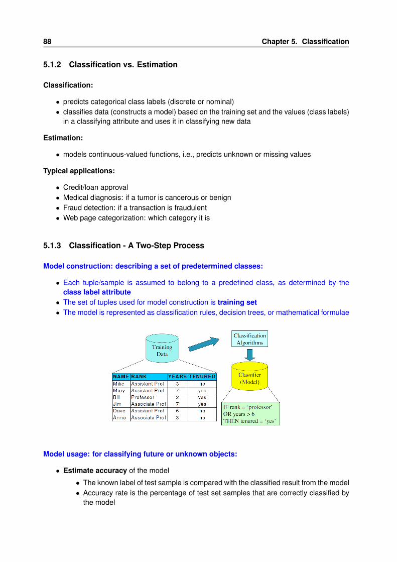
88 Chapter 5. Classification
5.1.2 Classification vs. Estimation
Classification:
• predicts categorical class labels (discrete or nominal)• classifies data (constructs a model) based on the training set and the values (class labels)
in a classifying attribute and uses it in classifying new data
Estimation:
• models continuous-valued functions, i.e., predicts unknown or missing values
Typical applications:
• Credit/loan approval• Medical diagnosis: if a tumor is cancerous or benign• Fraud detection: if a transaction is fraudulent• Web page categorization: which category it is
5.1.3 Classification - A Two-Step Process
Model construction: describing a set of predetermined classes:
• Each tuple/sample is assumed to belong to a predefined class, as determined by theclass label attribute• The set of tuples used for model construction is training set• The model is represented as classification rules, decision trees, or mathematical formulae
Model usage: for classifying future or unknown objects:
• Estimate accuracy of the model
• The known label of test sample is compared with the classified result from the model• Accuracy rate is the percentage of test set samples that are correctly classified by
the model

5.1. Basic concepts 89
• Test set is independent of training set, otherwise over-fitting will occur
• If the accuracy is acceptable, use the model to classify data tuples whose class labels arenot known
5.1.4 Issues
5.1.4.1 Data Preparation
• Data cleaning: Preprocess data in order to reduce noise and handle missing values• Relevance analysis (feature selection) : Remove the irrelevant or redundant attributes• Data transformation : Generalize and/or normalize data
5.1.4.2 Evaluating Classification Methods
• Accuracy
• classifier accuracy: predicting class label• predictor accuracy: guessing value of predicted attributes
• Speed
• time to construct the model (training time)• time to use the model (classification/prediction time)
• Robustness: handling noise and missing values• Scalability: efficiency in disk-resident databases• Interpretability : understanding and insight provided by the model• Other measures, e.g., goodness of rules, such as decision tree size or compactness of
classification rules

90 Chapter 5. Classification
5.2 Decision tree induction
5.2.1 Introductory example
5.2.1.1 Training dataset
Let’s consider this training datasets:
• What attribute to take in consideration and in what order ?• Problem: one cannnot generate every possible tree to answer this question...
5.2.1.2 Sample expected decision tree
We are looking for the attributes which provide the best split of the data, for instance:
5.2.2 Algorithm for Decision Tree Induction
Basic algorithm (a greedy algorithm)
• Tree is constructed in a top-down recursive divide-and-conquer manner

5.2. Decision tree induction 91
• At start, all the training examples are at the root• Attributes are categorical (if continuous-valued, they are discretized in advance)• Examples are partitioned recursively based on selected attributes• Test attributes are selected on the basis of a heuristic or statistical measure (e.g., infor-
mation gain)
Conditions for stopping partitioning
• All samples for a given node belong to the same class• There are no remaining attributes for further partitioning - majority voting is employed for
classifying the leaf• There are no samples left
5.2.2.1 Algorithm
Notation:
• Let D be set of tuples with their attributes.• Let C be the target classification which we want to achieve, and Ci (i=1..m) a class in C
(C contains m classes)• Let A be whatever attribute providing a classification of the elements in D. A contains v
classes.
Definition:
• The Expected Information (entropy) needed to classify a tuple in D:Info(D) = −
∑mi=1 pilog2(pi)
• where pi be the probability that an arbitrary tuple in D belongs to class Cipi can be estimated as pi =
|Ci,D||D|
• The Information needed (still needed) after using A to split D into v partitions to classifyD:InfoA(D) =
∑vj=1
|Dj ||D| × InfoA(Dj)
• where InfoA(Dj) is the expected information (entropy) needed to clas-sify a tuple (according to the target attribute) in Dj : InfoA(Dj) =
−∑m
i=1 p(i→Dj)log2(p(i→Dj))
• where p(i→Dj) be the probability that an arbitrary tuple in Dj belongs to classC(i→Dj)
p(i→Dj) can be estimated as p(i→Dj) =|Ci,Dj
||Dj |
• The Information gained by branching on attribute A is Gain(A) = Info(D)− InfoA(D)
Algo:
1. Compute the expected information (entropy) neeed to classify a tuple in D as

92 Chapter 5. Classification
(a) The expected information Info(D) is computed byInfo(D) = −
∑mi=1
|Ci,D||D| log2(
|Ci,D||D| )
2. Compute information gain (entropy) for each attribute A (except C - the target attribute):For each attribute A, compute Information Gained by branching on AGain(A)
(a) Compute each InfoA(Dj) where j=1.."number of classes of A"
InfoA(Dj) = −∑m
i=1
|Ci,Dj|
|Dj | log2(|Ci,Dj
||Dj | )
(b) Compute Information needed after using A to split D into v partitions toclassify D:InfoA(D) =
∑vj=1
|Dj ||D| × InfoA(Dj)
(c) The Information gained by branching on attribute A is Gain(A) = Info(D) −InfoA(D)
3. Select the attribute with the highest information gain (highest entropy):→ use the values computed above and select the attribute with the highest one.
4. The first level of classifications becomes this attribute. From the current node (whichmight be the root node one the first iteration), create branches for each value oif thisattibute.
5. Then for each of these new branches, apply this algorithm recursively starting with point2, as if the root node has become the current branch and the new set D has becomethe subset of D thus computed.(The split might well be a different attribute for each branch.)
6. The recursion stops when every element of the specific branch have the sameresults!
5.2.2.2 Example
→ Using the example provided in 5.2.1.
Compute expected information:
• First let’s count the elements in each group:
• |c = yes| = 9
• |c = no| = 5
• Thus Info(D) = − 914 log2(
914)− 5
14 log2(514)
Compute Gain(age)
• Age is splitted in three classes: below = age <= 30 → j = 1, middle = 31 >= age < 40
→ j = 2 and above = age >= 40→ j = 3 :
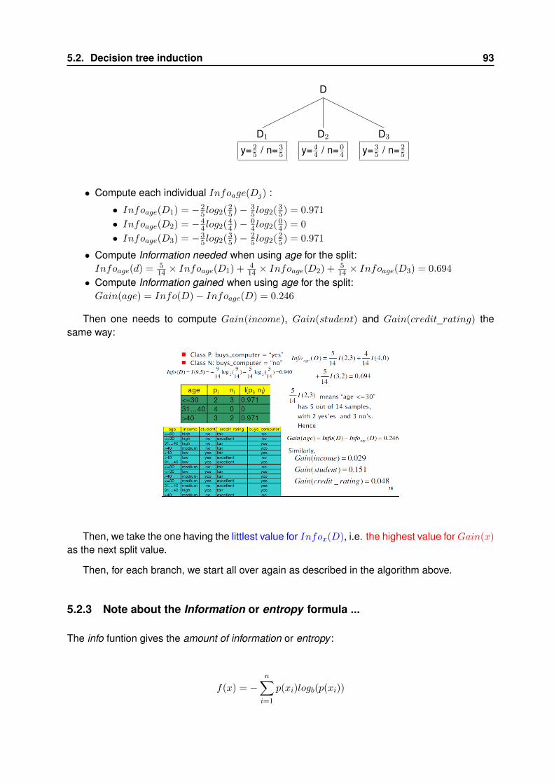
5.2. Decision tree induction 93
D
D1
y=25 / n=3
5
D2
y=44 / n=0
4
D3
y=35 / n=2
5
• Compute each individual Infoage(Dj) :
• Infoage(D1) = −25 log2(
25)− 3
5 log2(35) = 0.971
• Infoage(D2) = −44 log2(
44)− 0
4 log2(04) = 0
• Infoage(D3) = −35 log2(
35)− 2
5 log2(25) = 0.971
• Compute Information needed when using age for the split:Infoage(d) = 5
14 × Infoage(D1) + 414 × Infoage(D2) + 5
14 × Infoage(D3) = 0.694
• Compute Information gained when using age for the split:Gain(age) = Info(D)− Infoage(D) = 0.246
Then one needs to compute Gain(income), Gain(student) and Gain(credit_rating) thesame way:
Then, we take the one having the littlest value for Infox(D), i.e. the highest value forGain(x)
as the next split value.
Then, for each branch, we start all over again as described in the algorithm above.
5.2.3 Note about the Information or entropy formula ...
The info funtion gives the amount of information or entropy :
f(x) = −n∑i=1
p(xi)logb(p(xi))

94 Chapter 5. Classification
or in our case :
f(x) = −xlogb(x)− (1− x)logb(1− x)
The usage of the info formula is a trick. What we want is a formula which returns the minimumvalue 0 when every single element are within the same class and the maximum possible valuewhen the values are well mixed amongst the two classes.And we get exactly that with the info forumla.
This is how the info curve looks like:
The function returns 0 when all elements are 1 or 0 (in the same class) and 1 when elementsare the most spread amonst the two classes.
This function is also called degree of disorder.
5.2.4 Computing information gain for continuous-value attributes
Whenever A is a continuous value, it must be discretized.
Determine the best split point for A:
• Sort the value A in increasing order• Typically, the midpoint between each pair of adjacent values is considered as a possible
split point :(ai + ai+1) / 2 is the midpoint between the values of ai and ai+1
• The point with the minimum expected information requirement for A is selected as thesplit-point for A
Split:
• D1 is the set of tuples in D satisfying A ≤ ”split− point”, and D2 is the set of tuples in Dsatisfying A > ”split− point”

5.2. Decision tree induction 95
5.2.5 Gini Index
The Gini Index method consists in using a differenign formula than the Information Quantity orEntropy we have been using before.
The Gini Index is used by the CART or IBM IntelligentMiner products.
Instead of the formulas we have been using before, we use the following below. And wealways built a binary tree, i.e. split the set of values for an attribute in two groups
• If a data set D contains examples from n classes, gini index, gini(D) is defined asgini(D) = 1−
∑ni=1 p
2i
• where pj is the relative frequency of class j in D
• If a data set D is split on A into two subsets D1 and D2, the gini index gini(D) is definedasginiA(D) = |D1|
D × gini(D1) + |D2|D × gini(D2)
• Reduction in Impurity:∆gini(A) = gini(D)− giniA(D)
• The attribute provides the smallest ginisplit(D) (or the largest reduction in impurity) is cho-sen to split the node (need to enumerate all the possible splitting points for each attribute)• All attributes are assumed continuous-valued• May need other tools, e.g., clustering, to get the possible split values• Can be modified for categorical attributes
The gini function has exactly the same shape than the entropy function seen above
5.2.5.1 Gini Index - example
• Ex. D has 9 tuples in buys_computer = “yes” and 5 in “no”gini(D) = 1− ( 9
14)2 − ( 514)2) = 0.459
• Suppose the attribute income partitions D into 10 in D1: low, medium and 4 in D2: high:giniincome∈{l,m}∪{h}(D) = 10
14 × gini(D1) + 414 × gini(D2))
where:
• gini(D1) = (1− ( 610)2 − ( 4
10)2)
• gini(D2) = (1− (14)2 − (34)2)
• Hence giniincome∈{l,m}∪{h}(D) = 0.450
• But giniincome∈{l}∪{m,h}(D) = 0.30 and thus is the best value since it is the lowest
5.2.6 Comparing attribute selection measures
The two measures, in general, return good results, but:
• Information gain: biased towards multivalued attributes• Gini index:
96 Chapter 5. Classification
• biased to multivalued attribute• has difficulty when number of classes is large• tends to favor tests that result in equal-sized partitions and purity in both partitions
5.2.7 Overfitting and Tree Pruning
Overfitting: An induced tree may overfit the training data
• Too many branches, some may reflect anomalies due to noise or outliers• Poor accuracy for unseen samples
Two approaches to avoid overfitting
• Prepruning: Halt tree construction early—do not split a node if this would result in thegoodness measure falling below a threshold.→ Difficult to choose an appropriate threshold• Postpruning: Remove branches from a “fully grown” tree—get a sequence of progressively
pruned trees.→ Use a set of data different from the training data to decide which is the “best prunedtree”
5.2.8 Classification in Large Databases
• Classification: a classical problem extensively studied by statisticians and machine learn-ing researchers• Scalability: Classifying data sets with millions of examples and hundreds of attributes with
reasonable speed• Why decision tree induction in data mining?
• relatively faster learning speed (than other classification methods)• convertible to simple and easy to understand classification rules• can use SQL queries for accessing databases• comparable classification accuracy with other methods
5.3 Model evaluation and selection
(Globaly outside the scope of the lecture, except the few details below)
Accuracy - definition:
Accuracy of a classifier M, acc(M): percentage of test set tuples that are correctly classified bythe model M
The holdout method:
• Training set (e.g., 2/3) for model construction

5.3. Model evaluation and selection 97
• Test set (e.g., 1/3) for accuracy estimation
A variation of the holdout method: random sampling:
• Repeat holdout k times, accuracy = avg. of the accuracies obtained

98 Chapter 5. Classification