31

Piyu Yue

Piyu Yue, a research associate at the IC2 Institute, University ofTexas at Austin, was a visiting scholar at the Federal ReserveBankof St. Louis when this article was written. Lynn Dietrichprovidedresearch assistance. The author would like to thank A.Charnes, Roll Fare and Shawna Grosskopf for theirconstructivecomments and useful suggestions. Their DEA computer code ledto a significant improvement ofthe paper

Data Envelopment Analysis andCommercial Bank Performance:A Primer With Applications toMissouri Banks

OMMERCIAL BANKS PLAY a vital role in theeconomy for two reasons: they provide a majorsource of financial intermediation and their check-able deposit liabilities represent the bulk of thenation’s money stock. Evaluating their overallperformance and monitoring their financial condi-tion is important to depositors, owners, potentialinvestors, managers and, of course, regulators.

Currently, financial ratios are often used tomeasure the overall financial soundness of a bankand the quality of its management. Bank regu-lators, for example, use financial ratios to helpevaluate a bank’s performance as part of theCAMEL system.1 Evaluating the economic perfor-mance of banks, however, is a complicatedprocess. Often a number of criteria such as

profits, liquidity, asset quality, attitude towardrisk, and management strategies must be consi-dered. The changing nature of the bankingindustry has made such evaluations even moredifficult, increasing the need for more flexiblealternative forms of financial analysis.

This paper describes a particular methodologycalled Data Envelopment Analysis (DEA), that hasbeen used previously to analyze the relative effi-ciencies of industrial firms, universities, hospitals,military operations, baseball players and, morerecently, commercial banks.2 The use of flEA isdemonstrated by evaluating the management of60 Missouri commercial banks for the period from1984 to 1990.~

1For more details, see Booker (1983), Korobow (1983) andPutnam (1983).2The name DEA is attributed to Charnes, Cooper and Rhodes(1978), for the development of DEA, see Charnes, et al.(1 985)and Charnes, et at. (1978); for some applications of DEA, seeBanker, et al. (1984), Charnes, et al. (1990) and Sherman andGold (1985).3Although there is vast literature analyzing competition andperformance in the U.S. banking industry (e.g., Gilbert (1984),

Ehten (1983), Korobow (1983), Putnam (1983), Wall (1983)and Watro (1989)), actual banking efficiency has receivedlimited attention. Recently, a few publications have used IDEAor asimilar approach to study the technical and scale efficien-cies of commercial banks (e.g., Sherman and Gold (1985),Charnes etal. (1990), Rangan et al. (1988), Aty et al. (1990),and Etyasiani and Mehdian (1990)).

a4~sIcs

flEA represents a mathematical programmingmethodology that can be applied to assess the effi-ciency of a variety of institutions using a variety ofdata. This section provides an intuitive explana-tion of the DEA approach. A formal mathematicalpresentation of flEA is described in appendix A; aslightly different nonparametric approach isdescribed in appendix B.

flEA is based on a concept of efficiency that iswidely used in engineering and the naturalsciences- Engineering efficiency is defined as theratio of the amount of work performed by amachine to the amount of energy consumed in theprocess. Since machines must be operatedaccording to the law of conservation of energy,their efficiency ratios are always less than or equalto unity.

This concept of engineering efficiency is notimmediately applicable to economic productionbecause the value of output is expected to exceedthe value of inputs due to the “value added” inproduction. Nevertheless, under certain circum-stances, an economic efficiency standard—similarto the engineering standard—can be defined andused to compare the relative efficiencies ofeconomic entities. For example, a firm can be saidto be efficient relative to another if it produceseither the same level of output with fewer inputsor more output with the same or fewer inputs. Asingle firm is considered “technically efficient” if itcannot increase any output or reduce any inputwithout reducing other outputs or increasingother inputs.4 Consequently, this concept of tech-nical efficiency is similar to the engineeringconcept. The somewhat broader concept of“economic efficiency,”on the other hand, isachieved when firms find the combination ofinputs that enable them to produce the desiredlevel of output at minimum cost.5

The discussion of the flEA approach will beundertaken in the context of technical efficiencyin the microeconomic theory of production. tnmicroeconomics, the production possibility setconsists of the feasible input and output combina-tions that arise from available production tech-nology. The production function (or productiontransformation as it is called in the case of multipleoutputs) is a mathematical expression for aprocess that transforms inputs into output. In sodoing, it defines the frontier of the productionpossibility set. For example, consider the well-known Cobb-Douglas production function:

(1) Y = AK~Ll~a,

where Y is the maximum output for given quanti-ties of two inputs: capital (K) and labor (Ii. Even ifall firms produce the same good (Y) with the sametechnology defined by equation 1, they may stilluse different combinations of labor and capital toproduce different levels of output. Nonetheless, allfirms whose input-output combinations lie on thesurface (frontier) of the production relationshipdefined by equation 1 are said to be technologi-cally efficient. Similarly, firms with input-outputcombinations located inside the frontier are tech-nologically inefficient.

DEA provides a similar notion of efficiency. Theprincipal difference is that the flEA productionfrontier is not determined by some specific equa-tion like that shown in equation 1; instead, it isgenerated from the actual data for the evaluatedfirms (which in flEA terminology are typicallycalled decision-making units or DMU5).6 Conse-quently, the flEA efficiency score for a specificfirm isnot defined by an absolute standard likeequation 1. Rather, it is defined relative to the otherfirms under consideration. And, similar to engi-neering efficiency measures, DEA establishes a“benchmark” efficiency score of unity that noindividual firm’s score can exceed. Consequently,efficient firms receive efficiency scores of unity,while inefficient firms receive DEA scores of lessthan unity.

4See Koopmans (1951).

~Thisis also named “allocative efficiency” because a profitmaximizing firm must allocate its resources such that thetechnical rate of substitution is equal to the ratio of the pricesof the resources. Theoretical considerations of atlocative effi-ciency can be found in the articles by Banker (1984) andBanker and Maindiratta (1988).

mated production function represents the average behavior offirms in the sample. Hence, the estimated production functiondepends upon the data for both efficient and inefficient firms.By imposing suitable constraints, these statistical procedurescan be modified to orient the estimates toward frontiers. Inthis manner, the frontier of the production set can be esti-mated econometrically.

°ltis common to estimate production functions using regres-sion analysis. When cross-section data are used, the esti-

33

In microeconomic analysis, efficient productionis defined by technological relationships with theassumption that firms are operated efficiently.Whether or not firms have access to the sametechnology, it is assumed that they operate on thefrontier of their relevant production possibilitiesset; hence, they are technically efficient by defini-tion. As a result, much of microeconomic theoryignores issues concerning technological ineffi-ciencies.

flEA assumes that all firms face the sameunspecified technology which defines theirproduction possibilities set. The objective of flEAis to determine which firms operate on their effi-ciency frontier and which firms do not. That is,flEA partitions the inputs and outputs of all firmsinto efficient and inefficient combinations. Theefficient input-output combinations yield animplicit production frontier against which eachfirm’s input and output combination is evaluated.If the firm’s input-output combination lies on theDEA frontier, the firm might be considered effi-cient; if the firm’s input-output combination liesinside the DEA frontier, the firm is consideredinefficient.

An advantage of DEA is that it uses actualsample data to derive the efficiency frontieragainst which each firm in the sample can beevaluated.~As a result, no explicit functional formfor the production function has to be specified inadvance. Instead, the production frontier is gener-ated by a mathematical programming algorithmwhich also calculates the optimal DEA efficiencyscore for each firm.

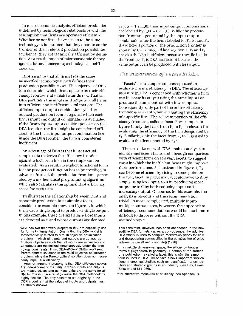
To illustrate the relationship between DEA andeconomic production in its simplest form,consider the example shown in figure 1, in whichfirms use a single input to produce a single output.In this example, there are six firms whose inputsare denoted as x, and whose outputs are denoted

as y~(i = 1,2,..,6); their input-output combinationsare labeled by F8 (s = 1,2 6). While the produc-tion frontier is generated by the input-outputcombinations for the firms labeled F1, F3, F5 and F6,the efficient portion of the production frontier isshown by the connected hne segments. F2 and F4are clearly flEA inefficient because they lie insidethe frontier; F6 is flEA inefficient because thesame output can be produced with less input.

hc. ..lmporiance of .rni.’eis in fJE~1

“Facets” are an important concept used toevaluate a firm’s efficiency in flEA. The efficiencymeasure in DEA is concerned with whether a firmcan increase its output using the same inputs orproduce the same output with fewer inputs.Consequently, only part of the entire efficiencyfrontier is relevant when evaluating the efficiencyof a specific firm. The relevant portion of the effi-ciency frontier is called a facet. For example, infigure 1, only the facet from F, to F3 is relevant forevaluating the efficiency of the firm designated byF2. Similarly, only the facet from F3 to F5 is used toevaluate the firm denoted by F4.8

The use of facets with flEA enables analysts toidentify inefficient firms and, through comparisonwith efficient firms on relevant facets, to suggestways in which the inefficient firms might improvetheir performance. As illustrated in figure 1, F2can become efficient by rising to some point onthe F,-F3 facet. In particular, it could move to A bysimply using less input, to B by producing moreoutput or to C by both reducing input andincreasing output- Of course, in this example, theanalysis is obvious and the recommendationtrivial. In more complicated, multiple input-multiple output cases, however, the appropriateefficiency recommendations would be much moredifficult to discover without the flEAmethodology.~

7DEA has two theoretical properties that are especially use-ful for its implementation. One is that the IDEA model ismathematically related to a multi-objective optimizationproblem in which all inputs and outputs are defined asmultiple objectives such that all inputs are minimized andall outputs are maximized simultaneously under the tech-nology constraints. Thus, IDEA-efficient DMUs representPareto optimal solutions to the multi-objective optimizationproblem, while the Pareto optimal solution does not neces-sarily imply DEA efficiency.Another important property is that IDEA efficiency scores

are independent of the units in which inputs and outputsare measured, as tong as these units are the same tor allIDMUs. These characteristics make the IDEA methodologyhighly flexible. The only constraint set originally in theCCR model is that the values of inputs and outputs mustbe strictly positive.

This constraint, however, has been abandoned in the newadditive IDEA formulation. As a consequence, the additiveIDEA model is used to compute reservation prices for newand disappearing commodities in the construction of priceindexes by Lovell and Zieschang (1990).81n a multiple dimensional space, the efficiency frontierforms a polyhedron. In geometry, a portion of the surfaceof a polyhedron is called a facet; this is why the sameterm is used in IDEA. These facets have important implica-tions in empirical studies, such as identification of compe-titors and strategic groups in an industry. See Day, Lewin,Salazar and Li (1989).°Foralternative measures of efficiency, see appendix B.

34

Figure 1Production Frontier and Efficiency Subset

Output Y

K

Scale E/!iciencv

In addition to measuring technological effi-ciency, flEA also provides information about scaleefficiencies in production. Because the measure ofscale efficiency in DEA analysis varies from modelto model, care must be exercised. The scale effi-ciency measured for the flEA model used in thisstudy, however, corresponds fairly closely to themicroeconomic definition of economics of scale inthe classical theory of production.’°

To illustrate, consider the F,-F3 facet in figure 2.Firms located on this facet exhibit increasingreturns to scale because a proportionate rise intheir input and output places them inside theproduction frontier. A proportionate decrease intheir input and output is impossible because itwould move them outside of the frontier. This isillustrated by a ray from the origin that passesthrough the F,-F3 facet at F’2.

Firms located on the F3-F3 facet exhibitdecreasing returns to scale because a propor-

tionate decrease in their input and output placesthem inside the production frontier. A propor-tionate increase in their input and output is impos-sible because it would move them outside of thefrontier.

Constant returns to scale occur if all propor-tionate increases or decreases in inputs andoutputs move the firm either along or above theproduction frontier. In figure 2, for example, F,exhibits constant returns to scale because propor-tionate increases or decreases would place itoutside the production frontier.

Since the facets are generated by efficient firms,the scale efficiency of these firms is determined bythe properties of their particular facet. Scale effi-ciencies for inefficient firms are determined bytheir respective reference facets as well. Thus, F2and F4 in figure 1 exhibit increasing anddecreasing returns to scale, respectively.

.LIEA and Ft’nr,mnk’ I1/1/ic1t?nr~t.~

While the discussion of flEA in the context oftechnological efficiency of production is useful forillustrative purposes, it is far too narrow andlimiting. flEA is frequently applied to questionsand data that transcend the narrow focus of tech-nical efficiency in production. For example, DEA isfrequently applied to financial data whenaddressing questions of economic efficiency. Inthis regard, its application is somewhat moreproblematic. For example, when firms facedifferent marginal costs of production due toregional or local wage differentials, one firm mayappear inefficient relative to another. Given thepotential differences in relative costs that a firmmay face, however, it might be equally efficient.Alternatively, differences that appear to be due toeconomic inefficiencies may in fact be due to costdifferences directly attributable to the non-homogeneity of products. Because of problemslike these, flEA must be applied judiciously.

.na1. g.J/j,,j0~1

To this point, the discussion of flEA has beenconcerned with evaluating the relative efficiencyof different firms at the same time. Those who useflEA, however, frequently employ a type of sensi-tivity analysis called“window analysis.” Theperformance of one firm or its reference firms

‘°SeeFare, Grosskopf and Lovell (1985). Different DEAmodels employ different measures of scale efficiency. See

F,

F, / F,

F,

0Input X

appendixes A and B for details,

Figure 2

An Illustration of Scale Efficiencies

OutputY

for a firm over time. Of course, comparisons offlEA efficiency scores over extended periods maybe misleading (or worse) because of significantchanges in technology and the underlyingeconomic structure.

0

may be particularly “good” or “bad” at a given timebecause of factors that are external to the firm’srelative efficiency. In addition, the number offirms that can be analyzed using the flEA model isvirtually unlimited. Therefore, data on firms indifferent periods can be incorporated into theanalysis by simply treating them as if theyrepresent different firms. In this way, a given firmat a given time can compare its performance atdifferent times and with the performance of otherfirms at the same and at different times. Througha sequence of such “windows,” the sensitivity of afirm’s efficiency score can be derived for a partic-ular year according to changing conditions and achanging set of reference firms.” A firm that isflEA efficient in a given year, regardless of thewindow, is likely to be truly efficient relative toother firms. Conversely, a firm that is only flEAefficient in a particular window may be efficientsolely because of extraneous circumstances.

In addition, window analysis provides someevidence of the short-run evolution of efficiency

APPLYING DEE TO BANKING:

AN EVALU.zVI’ION (IF’ 60 MISSOURI

(X)MJ.~IERCI.AL B

To demonstrate flEA’s use, it is applied toevaluate relative efficiency in banking. Financialdata for 60 of the largest Missouri commercialbanks for 1984 (determined by their total assets in1990) are used. Initially, the relative efficiency ofthese banks is examined using two alternativeflEA models: the CCII model and the additive flEAmodel. A discussion of these alternative DEAmodels appears in appendix A. In extending thediscussion and analysis, however, we focus solelyon the CCII model.

Measuring inputs and Outputs

Perhaps the most important step in using flEA toexamine the relative efficiency of any type of firmis the selection of appropriate inputs and outputs.This is partially true for banks because there isconsiderable disagreement over the appropriateinputs and outputs for banks. Previous applica-tions of flEA to banks generally have adopted oneof two approaches to justify their choice of inputsand outputs.’2

The first “intermediary approach” views banksas financial intermediaries whose primary busi-ness is to borrow funds from depositors and lendthose funds to others for profit. In these studies,the banks’ outputs are loans (measured in dollars)and their inputs are the various costs of thesefunds (including interest expense, labor, capitaland operating costs).

A second approach views banks as institutionsthat use capital and labor to produce loans anddeposit account services. In these studies, thebanks’ outputs are their accounts and transac-tions, while their inputs are their labor, capitaland operating costs; the banks’ interest expensesare excluded in these studies.

‘1This is called “panel data analysis” in econometrics.

‘2Some studies have adopted the simple rule that if itproduces revenue, it is an output; if it requires a net ex-

F, F,

F,F’,

F,

Input X

penditure, it is an input. For example, see Hancock (1989).

36

Our analysis of 60 Missouri banks uses a variantof the intermediary approach. The banks’ outputsare interest income (IC), non-interest income (N1C)and total loans (1’L). Interest income includesinterest and fee income on loans, income fromlease-financing receivables, interest and dividendincome on securities, and other income. Non-interest income includes service charges ondeposit accounts, income from fiduciary activitiesand other non-interest income. Total loans consistof loans and leases net of unearned income. Theseoutputs represent the banks’ revenues and majorbusiness activities.

‘I’he banks’ inputs are interest expenses (IE),non-interest expenses (NIE), transaction deposits(Tfl), and non-transaction deposits (NTD). Interestexpenses include expenses for federal funds andthe purchase and sale of securities, and the inter-est on demand notes and other borrowed money.Non-interest expenses include salaries, expensesassociated with premises and fixed assets, taxesand other expenses. Bank deposits are disaggre-gated into transaction and non-transaction depos-its because they have different turnover and coststructures. These inputs represent measures forthe banks’ labor, capital and operating costs. De-posits and funds purchased (measured by theirinterest expense) are the source of loanable fundsto he invested in assets.”

~ ~( fI••tissn’t.:ri. .tInnk

~/ I 1

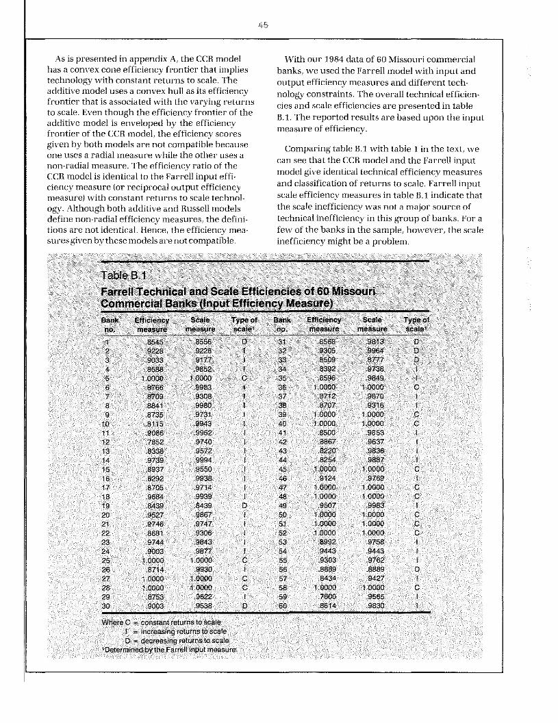
The flEA scores and returns to scale measuresresulting from applying the CCII and additive flEAmodels ar’e presented in table 1.” Although theoverall results are similar across the two models,there are minor differences in the individual effi-ciency scores that may provide information aboutthe relative efficiency of these banks.

The two models differ fundamentally in theirdefinition of the efficiency frontier. In particular,the CCII model assumes constant returns to scale,while the additive model allovvs for the possibilityof constant (C), increasing (I) or decreasing (fi)

returns. Because of this, banks that are efficient inthe CCII model must also he efficient in the addi-tive model. As table I illustrates for our Missouribanks, the converse, however, is not true.

The overall efficiency score is composed of“pure” technical and “scale” efficiencies. In theCCR model, a firm which is technologically effi-cient also uses the most efficient scale of opera-tion. In the additive model, however, the scorerepresents only “pure” technical efficiency. Bycomparing the results of the CCII and additivemodels, we can see that while five of our Missouribanks were technologically efficient, they werenot operating at the most efficient scale of opera-tion. The reader is cautioned, however, that thisanalysis excludes a number of factors (such asdemographic characteristics of the markets inwhich they operate) that may be important indetermining the most economically efficient scaleof operation.

Since the efficiency scores are defined differ-ently in the CCII and the additive flEA models, it isnot possible to generate a measure of scale ineffi-ciency using the results in table 1. Nevertheless,the fact that the efficiency scores from the twomodels are quite similar suggests that the scaleinefficiency is not a major source of overall ineffi-ciency for these banks. It appears that the ineffi-cient banks simply used too many inputs orproduced too few outputs rather than chose theincorrect scale for production.”

~ *‘flw( CI)‘.1.. ~ I.).’~ ~ .~

An illustration of the use of flEA analysis can heobtained by considering the data for the bankwith the lowest efficiency score, bank 59. Theresults for this hank are summarized in table 2.The reference banks making up the facet to whichbank 59 is compared and “lambda,” a measure ofthe relative importance of each reference bank inthe facet, are given. The table shows that threereference banks compose the facet for bank 59.Banks 51 and 39 play the major role and the otherbank is relatively unimportant.

“This is controversial, however. Some researchers specifydeposits as outputs, arguing that treating deposits as inputsmakes banks that depend on purchased money look artifi-ciallyefficient (see Berg et al., 1990).

“The results from solving the DEA model also include informa-tion about DEA scale efficiencies, the efficient projection onthe efticiency frontier, slack variables s,’ and s, - and the dualvariables Yr and u,. The “dual” variables represent “shadowprices” for each input and output. That is, they represent the

marginal effects of the input and output variables on thebank’s DEA efficiency score. See appendixA for details.

“Similar results of insignificant scale-inefficiency of U.S. bankshave been reported by Aly et al. (1990).

Table 1Overall Performance of 60 Missouri Commercial BanksEvaluated by the CCR and Additive DEA Models (1984)

Efficiency Ratio Efficiency Ratio

Bank CCR Additive Type of Bank CCR Additive Type ofno. model -. model scale’ no. model model scale’

8545 .8825 0 31 .8568 9310 D2 .9228 I 0000 I 32 .9305 9537 D3 .9033 9129 I 33 .8509 .8642 D4 .8588 9498 I 34 8392 .95545 1.0000 1.0000 C 35 .8596 89866 .8766 9042 I 36 1.0000 1 0000 C7 .8709 9144 I 37 8712 .98138 8841 9323 I 38 .8707 .9150 I9 8735 .9857 I 39 1.0000 1 0000 C

10 8115 9116 I 40 1.0000 1.0000 C11 9086 9856 I 41 8500 945312 7852 8388 I 42 .8867 .9656 I13 8338 .9927 I 43 .8220 .896514 9739 .9024 I 44 .8254 906915 .8937 9829 I 45 1 0000 1 0000 C16 .8292 8492 I 46 .9124 988917 8705 8211 I 47 10000 10000 C18 9684 .9783 I 48 10000 1.0000 C19 .8439 1.0000 D 49 .9507 9890 I20 .9527 9930 I 50 1 0000 1 0000 C21 9746 10000 I 51 1.0000 1.0000 C22 8681 .8888 I 52 1.0000 1.0000 C23 .9744 9642 I 53 .8992 9705 I24 9003 9646 54 9443 1.000025 1 0000 1.0000 C 55 .9303 .993126 8714 .8406 I 56 8889 1.0000 027 1.0000 1 0000 C 57 8434 933828 1.0000 1.0000 C 58 10000 10000 C29 8753 9351 I 59 7600 782430 9003 .93I9 D 60 .861~ .9541 I

Scale efficiency is measured by the CCR modelC = corlsla’it returns to scale

= ,ncroasinq returns to scaleD = decreasing returns to scaleDetermined by the CCR model.

I he ~aIur niraswr in the lint column in he I able 2 ako prescols LI rnea~ure or h,mk illlonri half cit the table ~ius the ~aloe of We denoli’d as he dual -l his measure is impurtanioutputs and the input— Inc bank .19 in 11151. liii- berau~r he ratio ol the duals or- outpuK andsecond rultnoo gi~es thr~aloe mr.hurr that hank inputs ~ s the I radent I of increments Or derre—.111 noold ha~rIn arhre~ein order to hi’ RI. \ dli— merits in inputs and otilputs to Dl. \ rIljcienc~

he tlilierence brlueen Ihese numbers i~ I his H ~ jIb lilt’ as~uniptinn that hid hank is tree to

presented in the third column ‘‘ Rank 513 shnukl ~an oil it its inputs anci outputs. I he lad that theocr-ease its total loans In 113 percent arid its non— dual lot \ll. is larue relalke lu the nIliei’,~i’’Psls

mien’,! income In Ii per ol Rank .59 should that the biggest elIicienr~gains hit hank .19 u illr edut-e its I our inpots h~2U.ti perrent oF interest comet rum derrea~ing non—inti’resi e\penses.e\penses and In 2-I perce nl of the other inputs, similar anal\ sk can hr cundot-ted for each joel Ii

‘i-i the case ci oarpus this c,if4

ere-ice is a measup ofslacK In tie case o’ rpuIs nowev~r.tie sacK variaDle

~, ri~recomplicated

38

cient bank to determine its reference banks andthe way in which it can become DEA efficient.

Table 24 (/<($~ 4

Detailed Results for Bank 59The available data cover a seven-year span from Efficiency Score = .7600

1984 through 1990. A three-year period was Facet 51 39 27chosen to allow five windows. The windows and Lambda = .315 188 037the periods they cover are as follows:

Value Value ifwindow 1 1984 1985 1986 Outputs measures efficient Difference Dualwindow 2 1985 1986 1987 IC 9.627,0 9627.0 .0 .7895E-04window 3 1986 1987 1988 NIC 350.0 371.9 21.9 i000EO8window 4 1987 1988 1989 TL 22.4420 54,599.8 32,157.8 .3704B10

windowS 1988 1989 1990 inputslE 7.887,0 5.7843 2.1027 .4762E-09

In each window) the number of banks is tripled NIE 2.1 82.0 1 658 4 523 6 2277E-03because each bank at a different year is treated as 19,915.0 15.136,0 4.7790 2780E-05

an independent firm. Repeating the procedure NTO 77.0050 58526.1 18478.9 .5815E-05

discussed above for each window, informationabout the evolutions of DEA efficiencies of every well as that of other banks. The distribution ofbank during the seven-year period was obtained, banks by their average efficiency over the fiveTable 3 lists the DEA scores of three banks by year windows is presented in table 4.in each window. The average of the 15 DEA effi-ciency scores is presented in the column denoted Bank 48 was the only one that was efficient for“mean.” The column labeled GD indicates the every year in every window over the 1984-90greatest difference in a bank’s DEA scores in the period. Its average efficiency of 1.00 indicates thatsame year but in different windows. The column bank 48 was a superb bank in the sample DEAlabeled TGD denotes the greatest difference in a evaluation.bank’s DEA scores for the entire period.

Bank 41, on the other hand, began in the firstA bank can receive a different DEA efficiency window with scores of 0.84 in 1984, 0.85 in 1985

score for the same year in different windows. This and 0.89 in 1986. In the second window, bank 41variation in the DEA scores of each bank reflects had scores of 0.86 in 1985, 0.90 in 1986 and 0.94 inboth the performance of that bank over time as 1987. Although all of its efficiency scores fluctu-

Table 3DEA Window Analysis

______ Efficiency Scores Summary Measures

Sank YR84 YRBS Y986 VRB1 YR8S YR89 YR9O MEAN GD TGD

48 1 00 1 .00 1.00 1.00 0.00 0.001.00 100 1.00

1.00 100 1001.00 1.00 1.00

1.00 100 1.00

41 0.84 085 0.89 0.92 0.05 0 140.86 0.90 0.94

090 0.94 091096 094 0.96

0.96 0.98 0.9859 0.76 068 0.60 0.68 004 0 18

0.70 060 0.630.59 063 067

0.65 0.70 0.750.71 076 077

39

Table 4Distribution of Average DEA Scores(1984-1990)

Five-year average NumberModel DEA score of banks

CCR 1.00098-099 80.96—0.97 40.93—0.95 130.91—092 7

090 3088.-Gag 40.86—0.87 10083—085 5080-- 082 3

0.79 10.68 1

ated slightly in the other three windows, theytended to increase. With a gradual improvementin its DEA efficiency over the seven years, bank 41was almost fully efficient in the last year, with aDEA score of 0.98. However, its average-efficiencyscore of 0.92 does not put it among the top 13banks for the period.

In contrast to the banks previously discussed,bank 59 displayed relatively erratic and inefficientbehavior over the entire seven-year period. Itsaverage DEA score of 0.68 was the lowest of the60 Missouri banks analyzed.

The window analysis enables us to identify thebest and the worst banks ina relative sense, aswell as the most stable and most variable banks interms of their seven-year average DEA scores.

:flNTJ4JLJflJG REM.%1t.K.S

The DEA methodology discussed in this articlehas the potential to provide crucial informationabout banks’ financial conditions and managementperformance for the benefit of bank regulators,managers and bank stock investors. The flEAframework is extremely general, permittingmultiple criteria for evaluation purposes.Moreover, flEA requires only data on the quantityof inputs and outputs; no price data are necessary.This is especially appealing in the analysis ofbanking because of the difficulties inherent indefining and measuring the prices of banks’ inputsand outputs.

In addition, the DEA method is highly flexible. In

considerably fewer limitations than alternativeeconometric approaches. Nevertheless, if the anal-ysis is tobe useful, care must be exercised in theselection of inputs and outputs.

•17NC ES.

Ahn, T., A. Charnes, and W. W. Cooper. “Some Statistical andDEA Evaluations of Relative Efficiencies of Public andPrivate Institutions of Higher Learning,” Socio-EconomicPlanning Sciences, Vol. 22, No. 6, 1988, pp. 259-69.

_______- “Efficiency Characterizations in Different DEAModels,” Socio-Economic Planning Sciences, Vol.22, No.6,1988, pp. 253-57.

Aly, Hassan V., Richard Grabowski, Carl Pasurka, and NandaRangan. “Technical, Scale, and Atlocative Efficiencies inU.S. Banking: An Empirical Investigation,” Review ofEconomics and Statistics (May 1990), pp. 211-18.

Amel, D., and L. Froeb. “Do Firms Differ Much?” Finance &Economics Discussion Series, Federal Reserve Board, #87August 1989.

Banker, Rajiv D. “Estimating Most Productive Scale Size UsingData Envelopment Analysis,” European Journal ofOpera-tional Research 217(1984), pp. 35-40.

Banker, Rajiv D., A. Charnes and W. W. Cooper. “Models forEstimating Technical and Scale Efficiencies,” ManagementScience, Vol. 30, (1984), pp. 1078-92.

Banker, Rajiv D., R. F. Conrad and R. P. Strauss.”A Compara-tive Application of DEA and Translog Methods: An IllustrativeStudy of Hospital Production,” Management Science Vol.36(1986), pp. 30-34.

Banker, Rajiv D., and Ajay Maindiratta. “Nonparametric Anal-ysis of Technical and Altocative Efficiencies in Production,”Econometrica (November1988), pp.1315-32.

Berg, S. A., F. R. Forsund, and E. S. Jansen. “Deregulation andProductivity Growth in Norwegian Banking 1980-1988: ANon-parametric Frontier Approach,” (Bank of Norway, 1990).

Booker, Irene 0. “Tracking Banks from Afar: A Risk MonitoringSystem,” Federal Reserve Bank of Atlanta Economic Review(November 1983), pp. 36-41.

Bovenzi, John F., James A. Marino, and Frank E. McFadden.“Commercial Bank Failure Prediction Models,” FederalReserve Bank of Atlanta Economic Review (November 1983),pp. 14-26.

Charnes, A., W. W. Cooper, B. Golany, L. Seiford and J. Stutz.“Foundations of Data Envelopment Analysis for Pareto-Koopmans Efficient Empirical Production Functions,”Journal of Econometrics (November 1985), pp.91-107.

Charnes, A., W. W. Cooper, Z. M. Huang and D.B. Sun. “Poly-hedral Cone-Ratio DEA Models with An Illustrative Applica-tion To Large Commercial Banks,” Journal of Econometrics(October/November 1990), pp. 73-91 -

Charnes, A., W. W. Cooper and E. Rhodes. “Measuring Effi-ciency of Decision Making Units,” European Journal of Oper-ational Research Vol. 1(1978), pp. 429-44.

Day, D. L., A. V. Lewin, R. J. Salazar, and H. Li. “StrategicLeaders in the U.S. Brewing Industry: A Longitudinal Anal-ysis of Outliers,” presented at the conference on New Usesof DEA, Austin, Texas, September 27-29, 1989.

Ehlen, James C. Jr. “A Review of Bank Capital and itsAdequacy,” Federal Reserve Bank of Atlanta EconomicReview (November1983), pp. 54-60.particular, the selection of inputs and outputs has

Elyasiani, Elyas, and Seyed M. Mehdian. “A NonparametricApproach to Measurement of Efficiency and TechnologicalChange: The Case of Large U.S. Commercial Banks,”Journal of Financial Services Research (July 1990),pp.157-68.

Fare, Rolf, Shawna Grosskopf, and C. A. K. Lovell. The Meas-urement ofEfficiency of Production (Kluwer-Nijhoff, 1985).

Fare, Rolf, and W. Hunsaker. “Notions of Efficiency and TheirReference Sets,” Management Science Vol.32 (February1986), pp. 237-43.

Gilbert, R. Alton. “Bank Market Structure and Competition. ASurvey,” Journal of Money, Credit, and Banking (November1984, Part 2), pp. 617-45.

Grosskopf, Shawna. “The Role of the Reference Technology inMeasuring Productive Efficiency,” The Economic Journal(June 1986), pp. 499-513.

Hancock, Diana. “Bank Profitability, Deregulation, and theProduction of Financial Services,” Research Working Paper89-16, Federal Reserve Bank of Kansas City (December1989).

Koopmans, T. C. “An Analysis of Production as an EfficientCombination of Activities,” mT. C. Koopmans, ed.,ActivityAnalysis of Production and Allocation, Cowles Commissionfor Research in Economics, Monograph No.13 (John Wileyand Sons, Inc., 1951).

Korobow, Leon, and David P. Stuhr. “The Relevance of PeerGroups in Early Warning Analysis,” Federal Reserve Bank ofAtlanta Economic Review(November 1983), pp. 27-34.

Lovell, C. A. K., and K. D. Zieschang. “A DEA Approach to theProblem of New and Disappearing Commodities in theConstruction of Price Indexes,” presented at the Sixth World

i%JJJfltCil dix AA (Join.parisou. 0! the C(AtTh~.•(7~flRatio itlonel

The most important characteristics of the flEAmethodology can he presented with the CCR RatioModel. Consider a gener’al situation where n deci-sion making units, UMUs, convert the same minputs into the same s outputs. The quantities ofthese outputs can he different for each DMU. Inmore precise notation, the j-th DMU uses am-dimensional input vector, ~ U = 1,2,...,m), toproduce an s-dimensional output vector, y,,~

(r = 1,2,..., s). The particular DMtJ being evaluatedis identified by subscript 0; all others are denotedby subscript 5. ‘the followingoptimization problemis formed for each DMU:

Max h0 = u,y~,I v,x~,

subject to the constraints:

‘1,

r~1 u,.y,.~/ ! v~x~ 1, u,. 0, v, 0

Congress of the Econometric Society, Barcelona, Spain,August 21-28, 1990.

Noonan, John H., and Susan Kay Fetner. “Capital and CapitalStandards,” Federal Reserve Bank of Atlanta EconomicReview (November 1983), pp.50-53.

Putnam, Barron H. “Concepts of Financial Monitoring,”Federal Reserve Bank of Atlanta Economic Review(November1983), pp. 6-13.

Rangan, Nanda, Richard Grabowski, Hassan V. Aly, and CarlPasurka. “The Technical Efficiency of U.S. Banks,”Economics Letters Vol. 28, No.2(1988), pp. 169-75.

Sherman, H. David, and Franklin Gold, “Bank Branch Oper-ating Efficiency: Evaluation with Data Envelopment Anal-ysis,”Journal of Banking and Finance (June 1985), pp.297-315.

Thrall, R. M. “Overview and Recent Development in DEA: TheMathematical Programming Approach,” paper presented atlC2 Institute, Conference Proceedings, University of Texas atAustin. October1989.

Wall, L. “Why Are Some Banks More Profitable Than Others?”Working Paper Series No. 12, Federal Reserve Bank ofAtlanta (November1983).

Watro, Paul R. “Have the Characteristics of High-EarningBanks Changed? Evidence From Ohio,” Economic Commen-tary, Federal Reserve Bank of Cleveland (September 1,1989).

Whalen, Gary. “Concentration and Profitability in Non-MSABanking Markets,” Federal Reserve Bank of ClevelandEconomic Review (1: 1987), pp. 2-9.

Zukhovitskiy, SI., and L. I. Avdeyeva. Linear and ConvexProgramming (W.B. Saunders Company, 1966).

where the output weights denoted by u,.(r = 1,2,..., s) and the input weights denoted by v1(i = 1,2 m) are required to he non.negative(i.e.,u,.,v~ 0forr = 1,2,..., s;i = 1,2 in).

The “virtual output” is the sum (I u,.yd) and the

‘‘virtual input’’ is the sum ( I x.’,x,~).The objective

function is defined by h,,, that is, the ratio ofvirtual output to virtual input. The solution is a setof optimal input and output weights. Themaximum of the objective function is the DEA effi-ciency score assigned to DMtJ0. The first set ofinequality constraints guarantees that the effi-ciency ratios of other DMUs (computed by usingthe same weights u~and v) are not greater thanunity. The remaining inequality constraints simplyrequire all input and output weights to be positive.Since every DMU can be DMUQ, this optimizationproblem is well-defined for every UMU. Becausethe weights (vi, ur) and the observations of inputsfori = 1,2,..., tn;r = 1,2 s;j = 1,2,..., n.

and outputs (x,1, y~j)are all positive and the con-straints must be satisfied by DMU0, the maximumvalue of h0 can only be a positive number less thanor equal to unity. If the efficiency score h0 = 1,

DMU0 satisfies the necessary condition to he flEAefficient; otherwise, it is flEA inefficient.

The above problem cannot he solved as statedbecause of difficulties associated with nonlinear(fractional) mathematical programming. Charnesand Cooper, however, have developed a mathe-matical transformation (the so-called “CC transfor-mation”) which converts the above nonlinearprogramming problem into a linear one. Existingduality theory and simplex algorithms in linearprogramming are used to solve the transformedproblein.1

For a linear programming problem, there existsa pair of expressions which are “dual” to eachother. The CCR ratio model is formed by problem1 and problem 2 below:

Problem 1:‘1’

Mm h,, = 0,, —c( I s~+ r~! s;)

subject to

00 x,,, — x,1 A1 — 5) = 0,

I y,.1 A~— 57 = yr,,’ A, 0, 57 ft s7 0,

fori = 1,..,m;r = 1,.., s;j = 1,..,n.

Problem 2:

MaxY0 = ,~, jA~y,.,,

subject to

V~ X11

, = ~ r-i PrYn , v,x,1 0,

Mr E, V1

E

tori = 1,..,m;r = 1,..,s;j = 1,..,n.

As before, the subscript 0 represents the UMU

being evaluated, x,1 denotes input i, y,.1

denotes

output r of DM1.)1, and ~1r and v, r’epresent the

weights for outputs and inputs, respectively. Anarbitrarily small positive number, , is introduced

to ensure that all of the observed inputs andoutputs have positive values or shadow prices andthat the optimal value h,, is not affected by thevalues assigned to the so-called “slack variables”

(s7 or s;1.2

The main conclusions from the CCR model aresun marized as follows:

1.The optimal values of 5;, s ;,and A, viaproblem I must be positive. The following inequal-ities should then he satisfied:

y’,.,, I y~A and 00x,0 I x,1 A1,

forr = 1,..., s;i = 1,..., in

2. Technical efficiency will he achieved if, andonly if, all of the following conditions are satisfied:

00 = land s = 0, s~= 0

fori = l,..,m;r = 1,..,s.

The condition 0,, = 1 ensures that DMUQ is locatedon the production frontier; the conditions 57 = 0

and s; = 0 exclude situations such as F6 in figure 1of the text.

3. The constant returns to scale condition for

DMU0 occurs if I A1 = 1, otherwise, I A, > I3 I—,

implies decreasing returns to scale; I A1 < I

implies increasing returns to scale.

4. An adjustment can be made in order to move(or project) inefficient DM1.)0 onto the efficiencyfrontier. The projection (1, y) in the CCR model isformed by the following formulas:

= 00x,0 — 5; i = 1, .., in

y,.0’ = y~0

+ s r = I, .., S.

The differences (x,0 x,,,), i = I,.., m, representamounts of inputs to be reduced; (y,.

0— yr,,),

r = 1 ,..,s, represent the amounts of outputs to beincreased in order to move DML’,, onto the effi-ciency frontier. Hence, these differences canprovide diagnostic information about the ineffi-ciency of DMU0.

‘This also opens the way for many different DEA modelswhich are refined, more flexible or more convenient forcomputations. These DEA models (BCC model, additiveDEA model, cone ratio DEA model, CCW model) and theirmathematical characteristics are beyond this paper.

2For the c-Method, see Zukhovitskiy et al, (1966), pp. 46-51.

42

5. Problem 1 is defined as the “primal” problemwhile problem 2 is the “dual.” The dual variableshave the economic interpretation of “shadowprices.” The value of i-’, indicates the marginaleffect of input x,,, on the PEA efficiency score. ‘[hevalue of Mr indicates the marginal effect of output

Yr on the PEA efficiency score. A comparison ofthese dual variables provides information on therelative importance of inputs and outputs in thePEA evaluation.

6. In the CCR model, problem I (or problem 2) issolved for each DMU. ‘rheoretically, ther’e is nolimitation on how many DMUs can enter the PEAmodel. Hence, the DEA model can perform an effi-ciency diagnosis for many DMUs.

Why is this approach referred to as dataenvelopment analysis? The two inequalities inconclusion 1,

y,.° I y,.,A1 and O,,xr,, ~

forr = I s;i = 1,..., in

are constraints to be satisfied for the optimal solu-tion. The fit-st inequality implies that the output ofDMU,, should not exceed the linear combination ofall observed output yr1 thus, the optimal solutionswill create a hyperplane to envelop the output ofDMU,, from above. Similarly, the second constraintcan be interpreted such that the optimal solutionscreate another hyperplane which envelops theinput of DMU0 from below. Since both outputsand inputs of the DMU evaluated are envelopedfrom above and below, the name PEAexactlymatches the geometric interpretation of theprocedure.

To see how this works, assume that there is agroup of DMUs that produces the same outputsusing the same inputs, but in varying amounts. Inranking their efficiencies of DMUs, PEA assignsweights to the outputs and inputs of each DMU.These weights are neither predetermined not’based on prior information or preferences of thedecision makers. Instead, each DMU receives a setof “optimal” weights that are determined bysolving the above mathematical programmingproblem. This procedure generates a PEA effi-ciency score for the DMU evaluated based on thesolution value for the input and output weights.A set of constraints guarantees that no DMU,including the one evaluated, can obtain an effi-

ciency score that exceeds unity. In this way, PEAderives a measure of the relative efficiency ratingfor each DMU in the cases of multiple input andoutput.

~J•:%iJiitii.i~ 4:Ittfl.1f?i

Among PEA models, the additive model hasbeen important in applications. The additivemodel can be formalized as the following twoproblems, which are dual to each other.~

Problem 3:

Max I s;/[x0[ + I S~/])J~~]1=3

subject to

x,0— I x,1A1— s; = 0, 1 YriAl_ s; YrO’

I A~ = 1, A~ °, 5; 0, 57 0,

for i = 1,.., m; r = 1,.., s; 5 = 1,.., n.

Problem 4:

Mm r~l M,Yro + I V1

X13

+

subject to:

r~i ~ + I v,x,1 + u0

0,

V1

1/ [x5[, Mr 11 ~y,.,,],

fori= l~.,m;r= 1,..,s;j= 1,..,n.

Compared with the CCR model, the additivemodel has introduced another constraint

A1 = I and a new variable u,,. The new

constraint in problem 3 ensures that the efficiencyfrontier is constructed by the convex combina-tions of original data points rather than a convexcone as in the CCR model. The new variable u0 inproblem 4 is used to identify returns to scale. Theother variables in the additive model haveinterpretations similar to the CCR model.

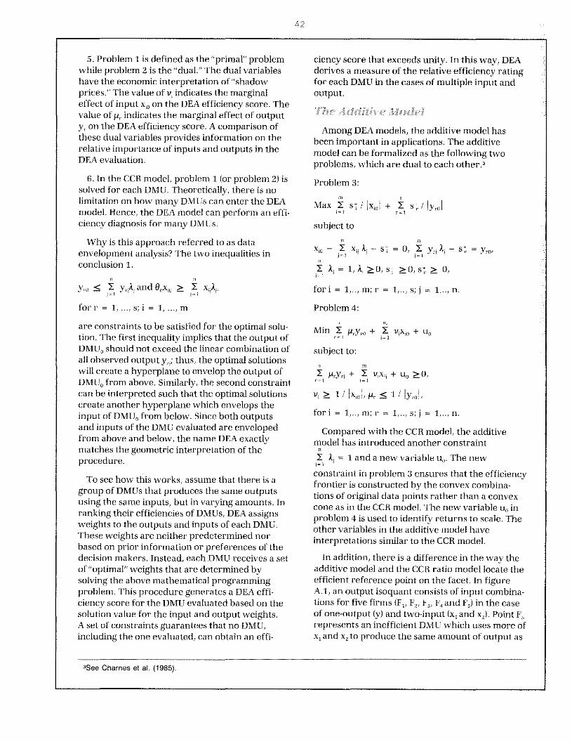
In addition, there is a difference in the way theadditive model and the CCR ratio model locate theefficient reference point on the facet. In figur-eAl, an output isoquant consists of input combina-tions for five firms (F, F2, F3, F,and F3) in the caseof one-output (y) and two-input (x, and x3). Point F,represents an inefficient DMLI which uses more ofx, and x,to produce the same amount of output as

3See Charnes et al. (1985).

4 ‘2

Input x,

to the intersection point B divided by the lengthfrom the origin to F,. In the additive model,however, the reference efficient point on facetF,-F,is denoted by A, which is determined bymaximizing the sum of the slacks, s, + 5,. Geometri-cally, the slack variables are expressed by thehorizontal line starting from F, and the verticalline extending to the facet F,-F,. Point A is selectedsuch that the sum of the lengths of the horizontaland vertical lines are maximized. The PEA effi-ciency score in the additive model that we used iscomputed by the following formula:

(I, 4 + r=3 ~ x,0 + r~1 yr,, + r~ 2s7).

where 4 and y,, are corresponding inputs andoutputs of the efficient reference point, such aspoint A.

The PEA scale efficiency in the additive model isidentified by a variable u,, in problem 4 in accor-dance with the followingcriteria:

If u0 = 0, DMU,, has constant returns to scale;otherwise,

its efficient reference DMUs, F, and F3. By the CCRratio model, the efficiency score is determined viaa value h0, which can be interpreted in terms ofthe ray from the origin to F,. That is, h0 is ex-pressed by the length of the ray from the origin

,‘i, n~n1erFsdh’v ii~t444

4,rlt,tA4.,1 24.

.,r .,,

u0 > 0 implies decreasing returns to scale;u0 < 0 implies increasing returns to scale.

The value of variable u,, is part of an optimal solu-tion of the additive model and is produced by thecomputer code such that facet rate =

C0( (~?7C7i7’f’~ ~ ~2’= \~t (;;i=;o,fl

In measuring and evaluating technical and scaleefficiencies there are two basic approaches: thePEA technique developed by Charnes, Cooper andothers in operations research and the approachdeveloped by Farrell, Fare and Grosskopf, amongothers, in economics.’ The latter approach isbased upon a set of axioms on production tech-nology to define the concept of efficiency. Someconnections of the two approaches have beeninvestigated by Banker, Charnes and Cooper(1984) and by Fare and Hunsaker (1986).

Both approaches share the characteristics thatthere is no need to specify a production functionor cost function and to estimate the parameters.Therefore, they are nonparametric, nonstochastictechniques that can be used toconstruct amultiproduct frontier relative to which the effi-ciency measures of the entities in the sample arecalculated. Because the frontier in theseapproaches is generated by data and all observa-tions are enveloped by the frontier, bothapproaches can be viewed as Data Envelopment

Figure A.1The Difference Between CCR and Additive DEA Models

Input xl,

F,

F,

0

F, F,

15ee Fare and Hunsaker (1986); Fare, Grosskopf andLovelI (1985).

44

Analysis. In this appendix, some of the differencesand similarities among the CCR and the additivemodels and the Farrell or Russell models arediscussed.

The choice of efficiency reference on the rele-vant frontier is a major difference among thesePEA models. In the Farrell or Russell models,three measures of technical efficiency can bedefined: input, output and graph efficiencymeasures.

Using the input efficiency measure, the ob-served output vector is fixed and the search forefficient reference is constrained to proportion-ally reducing inputs until the efficient frontier isreached. The “ratio of contraction,” as it is called,is the ratio of the particular input to be efficient tothe current level of inputs (in the Farrell inputmodel).

Using the output efficiency measure, the ob-served input vector is fixed and the outputs pro-portionally expanded until the efficient frontier isreached. ‘The “stretch ratio” of the output, as it iscalled, is the ratio of efficient output to the currentlevel of output (in the Farrell output model).

For the graph efficiency measure, both inputand output vectors are varied. Inputs are reducedand outputs are expanded, both proportionally,with the input ratio reciprocal to the output ratio.

In the case of figure 1 in the text, A is the refer-ence point for the input efficiency measure, B isthe reference point for the output efficiencymeasure and C might be the reference point forthe graph efficiency measure. These three effi-ciency measures can be classified as radialbecause proportional changes of inputs and/oroutputs are used in defining them.

To illustrate the input efficiency measure, rayOF3 in figure 1 of the text is used to represent theoptimal scale that would be generated by long-runcompetitive equilibrium. The overall input effi-ciency measure is defined with respect to the rayOF:,, while the input pure technical efficiency isdefined with respect to the line segment connect-ing F,, F, and F,. The measure of input overalltechnical efficiency, KP/KF,, can be decomposedinto the measure of pure technical input efficiencygiven by the ratio KA/KF, and the measure of inputscale efficiency given by the ratio KD/KA. When

the scale efficiency equals unity, the constant re-turns to scale occur; otherwise non-increasing orvarying returns to scale hold.

It is clear from these examples that, in general,these tadial efficiency measures will be different.Moreover, there is nothing to guarantee that afirm that is output efficient by this measure is alsoinput efficient or vice versa. For example, the firmdenoted by F6 in figure 1 of the text is output effi-cient by the output efficiency measure, but is notinput efficient (see Fare, Grosskopf and Lovell(1985)). Howevem-, the Farrell input efficiencymeasure is reciprocal to the Farrell output effi-ciency measure, if and only if, the technology ishomogeneous degree one. Because this conditionis satisfied by constant returns to scale tech-nology, the Farrell input and output efficiencymeasures are “identical” in this case. For modelswith other technologies, simple relationshipsbetween input and output efficiency measures donot hold.

An improvement of the Farrell or Russell modelsover the others is the use of non-radial efficiencymeasures. The use of proportional changes ofinputs and/or outputs in searching for efficientreference is abandoned.

Moreover, different piecewise linear technologycan be accommodated in both Farrell and Russellmodels to meet the needs of various users. Forexample, to measure scale efficiency we can useconstant returns to scale, non-increasing returnsto scale or varying returns to scale technologies.These technology constraints canbe easily imposedby corresponding restrictions on the “intensityparameters” in the Farrell or Russell models.

In the CCR or additive PEA model discussed inappendix A, however, only one efficiency measureis defined: the CCII model uses the radial measureof efficiency while the additive model uses thenon-radial measure.

Geometrically, the efficiency frontier with cons-tant returns to scale technology is a convex cone,but it is a convex hull in cases of both non-increas-ing and varying returns to scale. In general, theseconstraints on technology form a chain such thatone efficiency frontier is enveloped by another.Consequently, the associated efficiency measuresare compatible and nested.’

25ee Grosskopf (1986).

2~

~

to1

tJill

mID

o~

oow

ocoo~

coto

~

u~

~un~

nb~

tq~

—

(A—

(OoO

OD

O~

C,

c°’.O

DO

~41,~

O,

aA

~

fl~

*D

U0

a—

on

—n

—a

—o—

--—

~t~ 0

-g§~

ma

~~

‘.c~

flu

~~

sa8

8q

QQ

~.J

Qo

~Q

~o

*4

cq

o~

4p

.,o

N(D

QII

~

~~

-~

,..

~C

,~

Cow

—*

cO

wop~

ooath

OO

o~

oO

oow

~,c

oth

OO

—”J

OaC

A-4

GD

-~c

—C

Q~

OC

oo

~C

oo

co

QQ

Co

Q

——

O—

a—

——

000—

OO

—O

——

——

OO

——

O—

—000

a~

CD~C

C’

fl~

CCJ

Q—

,~

—-,

Pi

Cc

CDCD

~-,

CD-

~—

CD-

-,C

Di

C=

CCD

~C

D-~

-~>

;CC

~aC

Di~

0CD

Di

Cl

~-

CD<

CDC

CC’

~—

-~

-+

~c<

—C

D.

CD

0t

~—

C~

-tC

.~C

~—

CC

D

—.

~-C

~C

D~

C~

~<CD

OC

tCD

a-.

~CD

—.

C’

C -4

~~

CD

CC

EC

CC

flC

tCC

tCtC

’~C

DCA

=~

E-C

~—

~CD

-~j

CD

CC

DCD

00

k,

Cl

C’

CD.~

DiCD

~H

~~

~a

~D

iB

Ci

C~C

i—

a~

-g

a—

C~

C~

CCD

r*C’

Di

tCC

D_0

CD

~cC

~C

DC

C~C

at

—C

DCD

C~

C.

CC

’C CD&<

CD ~P

9~i

-‘e-

~~

‘~

—C

D_

CD

CC

CC

P~

CD~

~C

CD~

<C

D—

~C

go

~=

—~

-i~

-+z

~—C

C-=

;C

~+

Ct

aC<

g-q

—C

~C’

CDC

i—

~~.

CD~

<~

CCD

CD

—CD

CDC

i

~:~

c~!‘

~ C-~t6

~--

-~

CDC

<g

~b—.9

C~

CC

~-

a°CD

CCD

C’ a

-,C’

H9

a~B

~~

fl~

~C~

CD.

CD

CC

AC

i—~

Ci(A

Cl

?t~

—CD

Cl

9~

CC

Ca

CCD

CDC

C’

C—

~~C

DPi

QC

Cfl

CD

CD

CC

Ci

Cl~

Ci~

CC/

)—

CC

iCC

_~

+~

C~

Ci•

-“8

~~C

DC

D~C

CD

~CC

Ca

~‘tC

i~oC

Ca9

~~

~-t

CD

iCD

~-4

Ci4

~OO~OCD~

-Th

4tC

C’

CDC

~—

CC

CDCi

C~

CD

C’CD

~CD

~C

CC

a~

o9C

n~

BC

CD

C~

flC

DO

~~

rC

~C

D~

0C

,C’D

i-t—

~~

C_

.E~

9C

Dp

)-4

CA~

HCD

~‘i

pj

CD

BC

CiC

D—

~~

~alC

i*

Ct

CAD

~jC

CD

~z

C~

CADC

CD©

o9

DiC

iCC

D~

cCD

Cl—

~5

~~

ipi

CD

~CD

Ct

Cl

~~C

Dao

°ta

~C

D-C

DC

’ C~

-’~

aC

DC

CC

DZ

1~

a.

-+CD

C’

CD0

EE

~-~

E~

9r.r

1S

~C

DB

r*C

0C

ct

C’C

i0

C~

_~

DC

DCD

CDCD

CD—

CiCD

CiC

~C

’.-

,a

.CC

’~D

ioC’

0~Z

tC

i~~

CD

~9

Ci

CADCD

C

A